The probabilistic skill of extended-range heat wave forecasts over Europe

Severe heat waves lasting for weeks and expanding over hundreds of kilometers in the horizontal scale have many harmful impacts on health, ecosystems, societies, and the economy. Under the ongoing climate change, heat waves are becoming even longer and hotter, and, as a proactive adaptation, the development of early warning services is essential.

Weather forecasts in the extended range (2 weeks to 1 month) tend to indicate a higher skill in predicting warm extremes than average temperature events in Europe. We verified hindcasts of the European Centre for Medium-Range Weather Forecasts (ECMWF) in forecasting heat wave days, defined here as periods with the 5 d mean temperature exceeding its 90th percentile. The verification was done in 5° × 2° resolution over Europe, based on the forecast week (1 to 4 weeks). In the first forecast week, it is evident that, across Europe, the accuracy of ECMWF heat wave forecasts surpasses that of a climatological forecast. Even into the second week, in many regions in Europe, the ECMWF forecasts prove to be more reliable than their statistical counterparts. However, if we extend the forecast lead time to 3–4 weeks, predictability begins to decline to such a level that it can no longer be said, except for southeastern Europe, that the forecasts in general were statistically significantly better than the statistical forecast. Nonetheless, the persistence of prolonged heat waves seems to have a higher-than-average level of predictability even at a 3-week lead time, offering early warning services an indication of the potential duration of an ongoing heat wave.

1 Introduction

The severest heat waves in Europe since the 1950s have lasted for several weeks to even longer than a month, with horizontal spatial ranges exceeding several hundred kilometers, even 1000 km (Russo et al., 2015). In recent decades, the number of extreme heat waves over Europe and across the Northern Hemisphere has increased, and in the future, due to the ongoing climate change, heat waves are expected to become even more common and intense (IPCC, 2021; Russo et al., 2014; Coumou and Rahmstorf, 2012; Kim et al., 2018; Vogel et al., 2020; Ruosteenoja and Jylhä, 2023). This growing occurrence of heat waves underscores the urgent need to understand their dynamics and improve forecasting methods, especially for prolonged events with severe impacts.

Prolonged heat waves have negative impacts on, e.g., human health and well-being (Arsad et al., 2022; Guo et al., 2017; Ruuhela et al., 2021; Gasparrini et al., 2022; Kivimäki et al., 2023), labor productivity (Kjellstrom et al., 2009; Dunne et al., 2013; Orlov et al., 2019), energy and water resources (Añel et al., 2017; Hatvani-Kovacs et al., 2016; van Vliet, 2023), transport systems (Mulholland and Feyen, 2021), wildfire safety (Rossiello and Szema, 2019; Ruffault et al., 2020), agriculture (Heino et al., 2023; Vogel et al., 2019), and livestock (Ahmed et al., 2022; Morignat et al., 2014). As an example, during heat waves, apartments lacking air conditioning gradually begin to overheat, increasing heat stress (Velashjerdi Farahani et al., 2021, 2023, 2024a). In northern Europe, where apartments are typically not equipped with mechanical cooling systems, the thermal inertia of buildings plays a critical role. For instance, a Finnish study observed that buildings required 5–6 d to reach overheating conditions, highlighting the importance of the 5 d mean temperature as a predictor for indoor heat stress (Velashjerdi Farahani et al., 2024b). These findings emphasize the relevance of forecasting tools capable of predicting not only the occurrence but also the persistence of heat waves.

Prolonged and intensive heat waves occurring over a wide area can lead to significant and potentially catastrophic impacts on public health. In Europe, the 2003 heat wave has been estimated to have resulted in over 70 000 (Robine et al., 2008) and the 2022 heat wave in over 60 000 (Ballester et al., 2023) heat-related deaths. As climate change progresses, severe health effects of heat waves are expected to further increase (Guo et al., 2018). Recognizing this, many countries in Europe and other parts of the world have developed heat-health action plans over the past 20 years to mitigate heat-related health risks (Kotharkar and Ghosh, 2022; Martinez et al., 2022, 2019; Matthies et al., 2008). A key element of these preparedness plans consists of heat wave early warning systems, the operation of which is based on weather forecasts and pre-defined threshold criteria for triggering the warning services (Casanueva et al., 2019; Prodhomme et al., 2021). As health effects of heat exposure occur quickly, on the same day or with a lag of a few days (Baccini et al., 2008), it is imperative that the protection measures are implemented rapidly when a potentially dangerous heat wave is forecasted. However, organization of the response measures requires coordination of actions between many stakeholders and distribution of workforce, equipment, and other resources, which takes time. The effectiveness of the systems in preventing health effects depends on the ability to accurately forecast the impending heat event and the warning lead time. The lead time for heat wave warnings in each European country depends on the respective national meteorological and hydrological services. Currently, heat wave warnings across Europe are typically issued 2–5 d in advance, and in some countries, such as Germany and the UK, up to 7 d in advance. Extending these lead times could significantly enhance preparedness by allowing for earlier adaptive measures and better resource allocation, particularly for prolonged heat waves.

Sub-seasonal forecasts, which cover the extended range of 2 weeks to 1 month, offer a promising avenue for improving early warning systems. The skill of these extended-range forecasts has been found to be atmospheric-flow-dependent (Frame et al., 2013; Ferranti et al., 2015) and spatially heterogeneous. Vitart and Robertson (2018) highlighted the potential of sub-seasonal predictions in forecasting the progression of prolonged events like heat waves spanning multiple weeks. Moreover, Wulff and Domeisen (2019), and studies by Pyrina and Domeisen (2023), emphasized that extended-range predictions were more successful in forecasting extreme hot summer temperatures in Europe compared to predicting average summer temperatures.

Weather forecasts can be divided into two main categories: deterministic and probabilistic forecasts. Deterministic forecasts provide a single specific scenario for future weather. For example, “tomorrow will be hot” is a deterministic forecast that offers one possible future event. Probability forecasts, on the other hand, provide various possible scenarios and their associated probabilities, taking into account the uncertainty of the forecast. For instance, “50 % chance of heat” is a probability forecast indicating that heat may occur, but it is not certain. As the uncertainty of extended-range forecasts is known to be large, we evaluated their probabilistic rather than deterministic skill. In theory and practice, probabilistic forecasts have been shown to contain more information and should be more valuable to users than categorical, deterministic forecasts (e.g., Murphy, 1977; Richardson, 2001), though their practical utility depends on users' ability to incorporate such information into decisions (e.g., Lopez and Haines, 2017; Ramos et al., 2013).

Our objective was to assess the probabilistic skill of the extended-range forecasts made by the European Centre for Medium-Range Weather Forecasts (ECMWF) in predicting heat wave days, defined as periods when the local 5 d mean temperature exceeded the 90th percentile of the local summertime 5 d mean temperature distribution. We assessed the reliability of forecasts predicting heat waves surpassing this threshold, as this type of heat wave has been shown to significantly increase the risk of overheating in apartments in Finland (Velashjerdi Farahani et al., 2024a) and elevate mortality risk among the elderly (Kollanus et al., 2021). Our verification process was conducted using a resolution of 5° longitude and 2° latitude (5° × 2°) over Europe for the summers spanning 2000 to 2019. We examined hindcasts for various lead times, ranging from 1 to 4 weeks. The novelty of the study arises from the verification area encompassing the entirety of the European region, which allows us to highlight potential regional differences in the forecast skill, and from evaluating the model's ability to forecast the life cycle of heat waves, taking into account the forecast initialization date relative to the onset of the heat wave.

2 Data and methods

2.1 Definition of heat wave days

In this study, heat wave days were defined as periods when the local 5 d moving average temperature (T^5 d) exceeded its local summertime 90th percentile (90thT^5 d). To calculate T^5 d, local daily mean temperatures over land areas were averaged over a forward-looking 5 d window. The threshold 90thT^5 d was determined using summer data (June–July–August), ensuring that the definition reflected summertime extreme temperatures. By applying this threshold, the continuous variable T^5 d was converted into a binary variable: days were categorized as either heat wave days (T^5 d>90thT^5 d) or non-heat-wave days. In this study, heat wave days served as the forecast target. The choice of the 5 d moving average enables more robust identification of sustained heat wave events by reducing the influence of short-term variability. This is particularly important for extended-range forecasting, since such forecasts are not expected to skillfully predict small-scale, day-to-day variability.

Our definition of heat wave days is meaningful, as it aligns with thresholds commonly used in epidemiological studies on heat-related health effects, where heat waves are typically defined as periods when daily temperatures exceed the 90th percentile of the local annual or summertime temperature distribution for 2 or more consecutive days (Arsad et al., 2022). Such heat waves have been observed to lead to increased mortality and morbidity worldwide (Arsad et al., 2022; Guo et al., 2017). Although high temperature (dry bulb) is the primary variable for assessing heat wave impacts, other factors, such as humidity and wind speed, also contribute to heat stress. Nevertheless, this study focuses solely on temperature as the key driver of heat stress.

2.2 ERA5 data

2.2.1 Thresholds for heat wave days

For defining observed heat wave days with a horizontal resolution of 5° longitude and 2° latitude (5° × 2°) over Europe (36 to 70° N and −7.5 to 52.5° E) during summers 2000–2019, we used the ERA5 near-surface air temperature reanalysis data (Hersbach et al., 2020). The ERA5 data (Muñoz Sabater, 2019), with a horizontal resolution of 0.1°, were bilinearly interpolated to a 5° × 2° grid, considering only land grid points. To define heat wave days, we calculated the 5 d moving average temperatures ($T_{\mathrm{ERA}\mathrm{5}}^{\mathrm{5}\mathrm{d}}$) for each grid point across Europe during the summers of 2000–2019 and defined periods with $T_{\mathrm{ERA}\mathrm{5}}^{\mathrm{5}\mathrm{d}}$ exceeding its 90th percentile (90th$T_{\mathrm{ERA}\mathrm{5}}^{\mathrm{5}\mathrm{d}}$) as observed during heat wave days. Figure 1a depicts a map of the 90th percentile of the 5 d moving average temperature (in summers 2000–2019) over Europe, based on ERA5. Days having ERA5 5 d moving average temperatures above these thresholds, the 90th percentile, were, in this study, defined as observed heat wave days.

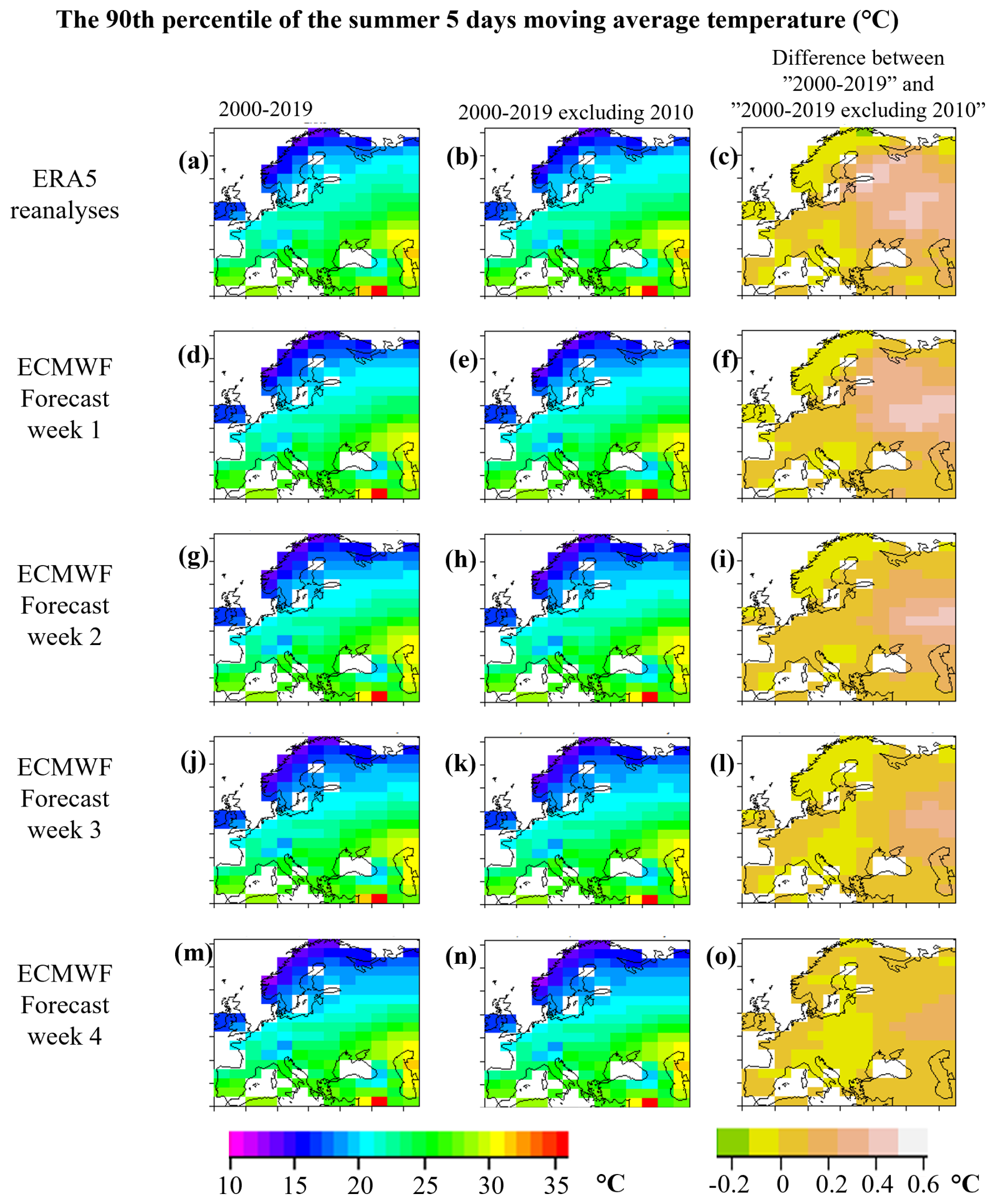
Figure 1 The lower thresholds of heat wave days: the 90th percentile of the 5 d moving average temperature in summers 2000–2019 (first column) and in summers 2000–2009 and 2011–2019 (i.e., 2000–2019 excluding 2010, middle column) of the ERA5 reanalyses (a, b) and (d, e, g, h, j, k, m, n) of the ensembles of the ECMWF's hindcasts in different forecast weeks. The last column shows the difference between these two.

As our definition of heat waves was based on 5 d mean temperatures, rather than daily mean temperatures, as commonly used in epidemiological studies on heat-related health effects, we examined the proportion of days where the daily mean temperature, the $T_{\mathrm{ERA}\mathrm{5}}^{\mathrm{1}\mathrm{d}}$, exceeded its 90th percentile (90th$T_{\mathrm{ERA}\mathrm{5}}^{\mathrm{1}\mathrm{d}}$) within periods when $T_{\mathrm{ERA}\mathrm{5}}^{\mathrm{5}\mathrm{d}}$ exceeded its 90th percentile, here defined as heat waves. For this, we computed daily mean temperatures, the $T_{\mathrm{ERA}\mathrm{5}}^{\mathrm{1}\mathrm{d}}$, and their 90th percentiles (90th$T_{\mathrm{ERA}\mathrm{5}}^{\mathrm{1}\mathrm{d}}$) across European land areas from 2000 to 2019. For each grid point, we determined the percentage of 5 d periods exceeding the 90th$T_{\mathrm{ERA}\mathrm{5}}^{\mathrm{5}\mathrm{d}}$ that included days where the $T_{\mathrm{ERA}\mathrm{5}}^{\mathrm{1}\mathrm{d}}$ exceeded its 90th percentile. Our analysis showed that our definition for heat waves based on exceeding the 90th$T_{\mathrm{ERA}\mathrm{5}}^{\mathrm{5}\mathrm{d}}$, covered 26 % of the 1 d heat waves based on exceeding the 90th$T_{\mathrm{ERA}\mathrm{5}}^{\mathrm{1}\mathrm{d}}$. For the 2 d heat waves based on exceeding the 90th$T_{\mathrm{ERA}\mathrm{5}}^{\mathrm{1}\mathrm{d}}$, our definition covered 61 %. The 3 d heat waves based on exceeding the 90th$T_{\mathrm{ERA}\mathrm{5}}^{\mathrm{1}\mathrm{d}}$ were covered 96 % by our definition. For 4 or more consecutive day heat wave events based on exceeding the 90th$T_{\mathrm{ERA}\mathrm{5}}^{\mathrm{1}\mathrm{d}}$, our definition covered 100 %. These statistics show that the 5 d moving average definition covers nearly all longer heat wave events (such as 3 to 4 d heat waves), but only a portion of shorter ones (1 to 2 d heat waves), indicating that the 5 d moving average is particularly useful for identifying sustained heat wave events.

During the period 2000–2019, the summer of 2010 was characterized by a particularly long-lasting heat wave over Europe (e.g., Trenberth and Fasullo, 2012). Therefore, we investigated the weight of this event on our results by comparing our results for the period 2000–2019 with and without the year 2010. Figure 1b gives a spatial distribution, with 1 °C intervals, for the threshold of the heat wave days for the period 2000–2019 excluding the summer of 2010. Figure 1c shows the impact of including 2010: in most of western and southern Europe, the difference is ±0.1 °C, while in eastern and northeastern parts of Europe the impact is mostly between 0 and +0.55 °C, except for very northern Fennoscandia where the impact is between −0.2 and 0 °C. Compared to the large northwest–southeast gradient of the absolute values of the 90th percentile in Fig. 1a and b, these differences are minor.

2.2.2 Frequency and duration of heat wave days

To identify the summer with the longest heat wave, we examined the frequency and duration of heat wave days in the ERA5 reanalysis data. A heat wave was considered to be any period of at least 1 d where the 5 d moving average temperature remained above the 90th percentile of $T_{\mathrm{ERA}\mathrm{5}}^{\mathrm{5}\mathrm{d}}$. The heat wave was considered interrupted when there were 2 consecutive days with temperatures falling below the 90th percentile of $T_{\mathrm{ERA}\mathrm{5}}^{\mathrm{5}\mathrm{d}}$. To clarify, a single day below the threshold did not end the heat wave, as long as it continued afterward.

The durations of the longest heat wave events in each grid point over Europe in summers 2000–2019, as derived from ERA5, are depicted in Fig. 2a. The heat wave events were longest in eastern Europe. Figure 2a highlights the extreme heat wave of 2010 in the east, the heat wave of 2018 in the north, and parts of central Europe and the heat wave of 2003 in parts of southern and southwest Europe. Figure 2b indicates that if the summer of 2010 is excluded, other years (e.g., 2014) appear in eastern Europe/western Russia, compared to Fig. 2a, and the duration of the longest period of heat wave days becomes shorter there. Figure 2c, showing the number of different heat wave events, highlights that in these summers (2000–2019) the heat wave days in northern Europe and in many parts of eastern Europe were concentrated within fewer periods, whereas in central and southwestern Europe, the same number of heat wave days was distributed across a larger number of periods. Figure 2d shows that if the summer of 2010 is excluded, especially in those areas where 2010 had the longest period of heat wave days, there is an increase in the number of periods with heat wave days, as 10 % of the hottest days are now distributed to a larger number of events.

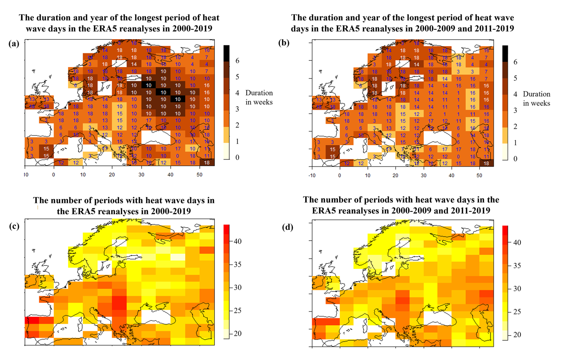
Figure 2 The duration and the year (marked as 0–19) of the longest period of heat wave days defined from the ERA5 reanalysis data of (a) summers 2000–2019 and (b) summers 2000–2009 and 2011–2019 (i.e., 2000–2019 excluding 2010) and the number of periods with heat wave days (c) in the ERA5 reanalyses during 2000–2019 and (d) 2000–2009 and 2011–2019 (i.e., 2000–2019 excluding 2010).

2.3 Hindcasts

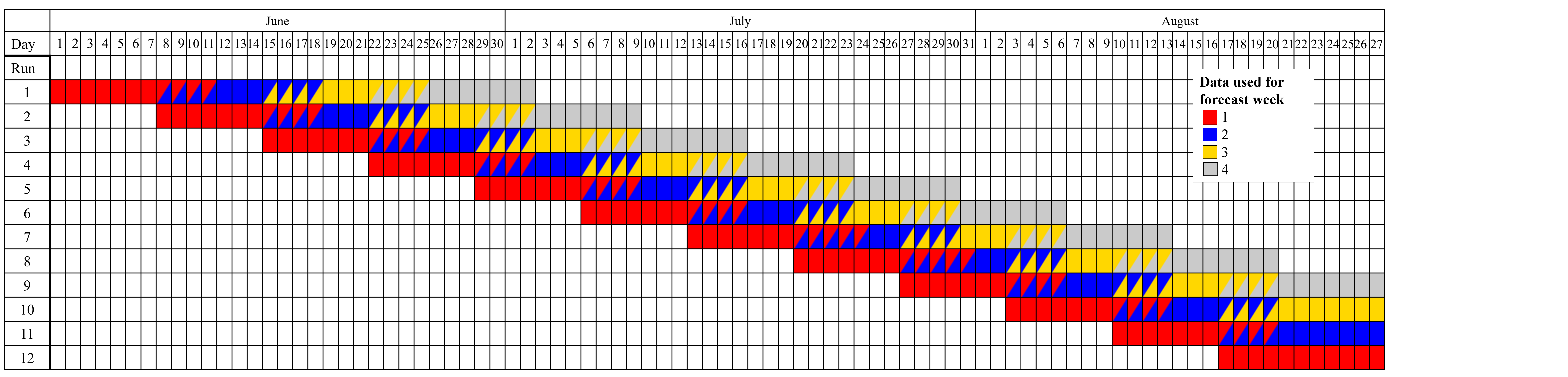
Hindcasts, also known as reforecasts, are a type of retrospective weather forecast. Hindcasts are forecasts of past weather conditions, generated using forecasting models, data assimilation methods, and observational data identical to those used for real-time weather predictions. Here, we verified hindcasts of the European Centre for Medium-Range Weather Forecasts (ECMWF) Integrated Forecasting System (IFS; Cycles 46r1 and 47r1; Vitart, 2014). These hindcasts were run at the ECMWF in 2020 twice a week, on Mondays and Thursdays, initialized using the ERA5 analyses. We investigated 240 hindcasts, which were run with a weekly interval for the summers 2000–2019, i.e., 20 years × 12 weeks =240 hindcasts; for details, see Table 1.

Table 1 This table shows the investigated hindcast data. Each row contains one run, a total of 12 runs per year. The coloring of the boxes shows the coverage of the hindcast data. The first red boxes on each row show the initialization date of the hindcasts, which are the same for all years 2000–2019. The colors of the boxes indicate for which lead time (i.e., forecast week) the data were used: red for 1 week, blue for 2 weeks, yellow for 3 weeks, and gray for 4 weeks. The data used for the different lead times were partially overlapping due to the use of 5 d moving averages with forward-looking window: a lead time of 1 week used data from days 1 to 11, 2 weeks used data of days 8 to 18, 3 weeks used data from days 15 to 25, and 4 weeks used data from days 22 to 32. The data used for two lead times are here marked with two colors. Note: for a lead time of 1 week, we used data of 12 runs; for 2 weeks, 11 runs; for 3 weeks, 10 runs; and for 4 weeks, 9 runs (per summer).

We examined the 2 m temperature (i.e., the near-surface air temperature) from the hindcasts with lead times of 1 to 32 d of the Monday runs. As the 2 m temperature has a large temporal autocorrelation, using both the Monday and Thursday initializations would not have added much information and would only have complicated the statistical analysis. We therefore arbitrarily decided to use only the Monday runs. The ECMWF reforecasts were initially run at a horizontal resolution of approximately 18 km for the first 15 d and then re-initialized at a coarser resolution of around 36 km for days 15 to 46. For our verifications, we used ECMWF's hindcasts at a horizontal resolution of 0.4°, which were bilinearly interpolated to a 5° × 2° grid, considering only land grid points.

The hindcasts consisted of a control forecast and 10 perturbed ensemble members, making up 11 members in total. It is important to distinguish between the hindcasts and the operational real-time forecasts, which initially had 51 members and now consist of 101 members (IFS Cycle 48r1). Consequently, the results obtained here from the 11-member hindcasts serve as a baseline measure of skill (see, e.g., Richardson, 2001; Ferro et al., 2008), and the larger operational ensemble is expected to provide improved estimates of the normal distribution parameters, thereby enhancing skill to some extent.

2.3.1 Thresholds for forecast heat wave days

For verification of the hindcasts, we defined the 5 d moving average temperatures in the ECMWF's hindcasts, $T_{\mathrm{EC}}^{\mathrm{5}\mathrm{d}}$. The calculations of $T_{\mathrm{EC}}^{\mathrm{5}\mathrm{d}}$ were performed separately for each of the 11 ensemble members, covering each day from 1 June to 27 August (88 d) over the summers of 2000–2019. For each day within this period, we incorporated forecast daily mean temperatures for that day and the subsequent 4 d into the calculations of $T_{\mathrm{EC}}^{\mathrm{5}\mathrm{d}}$. For each grid point and each forecast week, ranging from week 1 to week 4, we determined the threshold for a forecast heat wave day by calculating the 90th percentile, the 90th$T_{\mathrm{EC}}^{\mathrm{5}\mathrm{d}}$ , of the 5 d moving average temperatures, $T_{\mathrm{EC}}^{\mathrm{5}\mathrm{d}}$, from all days under consideration during the summers of 2000–2019. The forecast data used for the forecast weeks were partially overlapping due to the use of 5 d moving averages with forward-looking window: the forecast week 1 used data of days 1 to 11, the forecast week 2 data of days 8 to 18, forecast week 3 data of days 15 to 25, and forecast week 4 data of days 22 to 32, as depicted in Table 1.

In Fig. 1, the first column depicts maps of the 90th percentile of the 5 d moving average temperature (in the summers of 2000–2019) over Europe, based on ERA5 (Fig. 1a), and in the ECMWF hindcasts for forecast weeks 1–4 (Fig. 1d, g, j, and m). The ECMWF hindcasts capture the northwest–southeast gradient in the threshold of heat wave days. Although the absolute values in the hindcasts are somewhat lower than in ERA5 – with the difference increasing with lead time – this does not affect our verification, as we use model-specific thresholds.

Summer 2010 was marked by an unusually prolonged heat wave over Europe. In Fig. 1, the middle column depicts the spatial distribution of the thresholds for observed and forecast heat wave days over the period 2000–2019, excluding the summer of 2010. The last column of Fig. 1 (Fig. 1c, f, i, l, and o) illustrates the impact of including 2010. Compared to the large northwest–southeast gradient of the absolute heat wave day thresholds in the first two columns, the differences in the last column are minor. For assessing the impact of the summer of 2010 on the probabilistic skill of heat wave forecasts, the threshold values in the middle column are used.

2.3.2 Probability forecasts

The forecast probability of a heat wave day, p, was here based on fitting a normal distribution to the $T_{\mathrm{EC}}^{\mathrm{5}\mathrm{d}}$ forecasts of the 11-member ensemble (practically a set of deterministic forecasts) and defining the probability of the forecast $T_{\mathrm{EC}}^{\mathrm{5}\mathrm{d}}$ being above the 90th$T_{\mathrm{EC}}^{\mathrm{5}\mathrm{d}}$ on each day. Hence, a heat wave in the forecast is defined relative to the forecast model's climatology. The comparison of the hindcasts to the lead-time-dependent model climatology is expected to remove the systematic frequency bias resulting from the forecast model drift (Manzanas, 2020).

In the verification, the forecast model-based probability of a heat wave day, p, was compared to the observed heat wave days (Sect. 2.2.1), as derived from the ERA5 dataset. Since we used the data from the entire period (years 2000–2019) to define the heat wave day thresholds, we may achieve an overestimation of the forecast skill in the verification, compared to using a leave-one-out method (in which 1 year is excluded at a time from the dataset when defining the threshold). However, as shown in the last column of Fig. 1, excluding even the most extreme year has only a minimal impact on the threshold definition. Therefore, it is reasonable to assume that the effect on the skill is not substantial.

2.4 Skill scores

The Brier scores (BSs, Brier, 1950) of the probabilistic forecasts, p, were calculated separately for each grid point and forecast weeks 1 to 4 as follows:

$$\begin{array}{}\text{(1)}& \mathrm{BS}={\displaystyle \frac{\mathrm{1}}{N}}{\sum }_{t=\mathrm{1}}^N(p_t-o_t{)}^{\mathrm{2}},\end{array}$$

where p_t is the forecast probability of a heat wave day, ranging from 0 to 1, and o_t is the actual outcome (based on ERA5 reanalysis) of the heat wave day at instance t (0 if there is no heat wave day, and 1 if there is a heat wave day), and N is the number of forecasting instances. The BS is thus here equivalent to the mean squared error of the probability of a heat wave day, and ranges from 0 to 1. The lower the BS, the better the predictions.

It follows from the use of the 90th percentile to define a heat wave day (Sect. 2.2) that the expected probability p_b of a heat wave day is 0.1. This value, also referred to as the climatological base rate p_b, was used in Eq. (1) to calculate BS_ref, i.e., the Brier score of the reference forecast. The Brier skill score (BSS) can now be defined as

$$\begin{array}{}\text{(2)}& \mathrm{BSS}=\mathrm{1}-{\displaystyle \frac{\mathrm{BS}}{{\mathrm{BS}}_{\mathrm{ref}}}}.\end{array}$$

The value of the BSS ranges from −∞ to +1, whereas positive values indicate better skill than that of the reference forecasts, and a BSS value of 1 represents the best possible score.

Initially, we calculated the BSS for each grid point using data from all 240 hindcasts. To demonstrate the impact of long heat waves on the overall BSS of all hindcasts, we also determined the BSS while excluding the data from the summer with the longest heat wave (as detailed in Sect. 2.2.2). Importantly, this analysis was conducted separately for each grid point, acknowledging that the summer with the longest heat wave may vary from one grid point to another. Further, to demonstrate the impact of the summer of 2010 (with the long heat wave in Europe) on the probabilistic skill of the heat wave forecasts, we also determined the BSS while excluding data from summer 2010. Importantly, for this test, we excluded the 2010 data already when defining the thresholds for the heat wave days from the ERA5 and hindcast data, and hence, the thresholds were as in Fig. 1, in the middle column.

For each grid point and lead time, we determined whether the hindcasts were considered more skillful than the reference forecasts by assessing the BSS using a bootstrap resampling procedure. First, we calculated the BSS 5000 times, each time sampling the original data with replacement (i.e., the data points could be selected multiple times). The BSS was required to be statistically significantly above zero for the hindcasts to be considered more skillful than the reference forecasts. To assess this issue, we calculated the statistical significance level, i.e., the p value under the null hypothesis, that the BSS is zero. The p value is then the proportion of the bootstrap samples greater than zero. However, because the statistical test on the map is repeated many times, small p values are bound to occur by chance alone, and the null hypothesis is rejected too often. Unadjusted p values, therefore, overestimate the significance of the results (Wilks, 2016). We adjusted the p values following the false discovery rate (FDR) concept. The FDR-controlling procedures limit the expected proportion of false discoveries (hypotheses that should not have been rejected) among the rejected hypotheses. By setting this threshold q to 0.1, which is twice the conventional 0.05, as suggested by Wilks (2016), and using the Benjamini–Hochberg (B–H) procedure (e.g., Benjamini and Hochberg, 1995), we ensured that, on average, no more than 10 % of the rejected null hypotheses are false discoveries. In the B–H procedure, we first ordered the p values from the smallest to the largest. Then, we rejected the null hypothesis if $p_i<q\times i/m$, where i was the position, and m was the number of p values. In practice, we can use readily available p-value adjustment functions (such as p.adjust in R) that change p values to the smallest threshold q at which we would reject a particular null hypothesis.

3 Results

3.1 Reliability of probabilistic forecasts for heat wave days

First, we examined the proportion of heat wave forecasts in each category of forecast probabilities (p<0.1, $\mathrm{0.1}\le p<\mathrm{0.2}$, …, p≥0.9) (sharpness diagram in Fig. 3a) and how often heat wave days occurred following a forecast in each category of forecast probabilities (reliability diagram Fig. 3b). If all the forecasts were perfect, then in Fig. 3a, 90 % of the forecasts would have p=0 and 10 % would have p=1, and in Fig. 3b there would be only two points, [0,0] and [1,1], for each forecast week. However, for the first week, in Fig. 3a, roughly 80 % of the forecasts belong to the lowest probability class, and 5 % to the highest one. As the lead time increases, both these portions decrease, while the share of forecasts with $\mathrm{0.1}\le p<\mathrm{0.9}$ increases. The sharpness of forecasts drops as the lead time increases.

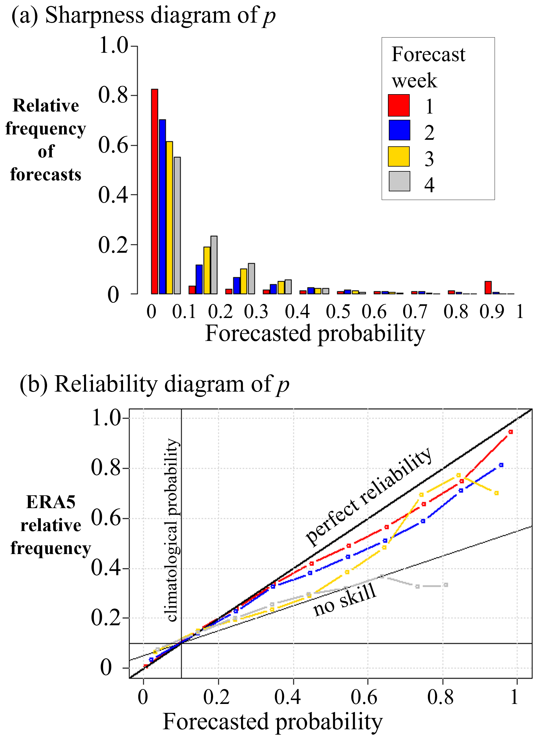
Figure 3 (a) The sharpness diagram and (b) reliability diagram of the 1–4 week probabilistic heat wave day forecasts, p, over Europe (all land grid points) in summers 2000–2019.

In Fig. 3b, the forecast probabilities are displayed on the x axis and observed frequencies on the y axis. In a perfectly calibrated forecast, the points on the reliability diagram would fall along a 45° diagonal line from the bottom left to the upper right corner. This line represents perfect reliability, where the forecast probabilities equal the observed frequencies. The climatological probability line in the reliability diagram represents the expected frequency of heat wave days (0.1) based on climatology. The points above the no skill line contribute positively to the BSS with climatology as the reference. The points on the reliability diagram above the perfect reliability line indicate underforecasting, meaning that the forecast probabilities are too low compared to the observed frequency. Conversely, the points on the reliability diagram below the perfect reliability line indicates overforecasting, meaning that the forecast probabilities are too high compared to the observed frequency.

The reliability of the heat wave day forecasts was best for shorter lead times and dropped with growing lead times (Fig. 3b). During forecast weeks 1 and 2, the overall reliability of heat wave day forecasts across Europe was nearly flawless when p<0.4. Subsequently, for p>0.4, the forecast probabilities tended to be slightly elevated compared to the observed frequencies, suggesting a tendency toward overforecasting; however, it should be noted that for lead times of 2 weeks (and longer), there are far fewer samples in the higher probability bins, making these points considerably more uncertain.

3.2 Probabilistic forecast skill scores for heat wave days

Figure 3b depicts the average reliability of the heat wave day forecasts over the whole of Europe. Next, we will take a look at the forecast skill across different regions in Europe to find out how the accuracy varies in different regions. First, we assess the performance of all the hindcasts of all summers from 2000 to 2019. Second, we examine hindcasts of summers from 2000 to 2019, excluding the hindcasts of the summer with the longest heat wave, and third, we focus on the hindcasts excluding the summer of 2010. In the first column of Fig. 4, we present the BSS of all hindcasts of the summers 2000–2019. During the first forecast week, the forecasts of heat wave days in Europe demonstrate strong performance, with BSS values ranging between 0.5 and 0.8. Based on the adjusted p values, these values of BSS are statistically significantly greater than 0 at every grid point. However, in later forecast weeks, the skill diminishes. In the second forecast week, the BSS ranges from 0.1 to 0.4 in Europe, the forecasts remain better than the reference forecast in most grid points across the continent. The exceptions include certain grid points over the northern parts of the Iberian Peninsula, eastern central Europe, and northeast of the Caspian Sea. Moving to forecast weeks 3 and 4, BSS values in Europe range between −0.1 and 0.2, exhibiting statistical significance only in specific grid points across eastern and southeastern Europe.

In the middle column in Fig. 4, we illustrate the BSS for each grid point of all hindcasts, excluding the summer with the longest heat wave (as defined in Sect. 2.2.2). The BSS excluding such a heat wave summer differs mostly only ±0.05 from the BSS of all summers, except in eastern Europe, where the BSS is even 0.1 lower in forecast weeks 2–4. In more detail, in the first forecast week, the BSSs of the hindcasts excluding the summer with the longest heat wave are between 0.4 and 0.7, and in all grid points, statistically significantly higher than 0, i.e., better than the reference forecast. In the second week, the BSS of the hindcasts excluding the summer with the longest period of heat wave days is between 0 and 0.4 and still statistically significantly higher than 0 in the majority of the grid points. In the third and fourth week, however, the BSS is statistically significantly higher than 0 only in some grid points in southeastern parts of the map.

In Fig. 4, the last column shows the BSS of the hindcasts excluding the summer of 2010. In some areas, leaving out 2010 seems to have less impact on the probabilistic skill of heat wave forecasts than leaving out, in each grid point, the summer with the longest heat wave (the middle column). For example, in Finland, the skill remains for the third week, and in the southeast parts of the study domain, the skill also appears to remain. These results suggest that the skill in forecasting heat waves decreased when excluding the longest period of heat wave days, whether it was the 2010 heat wave or a heat wave from another year.

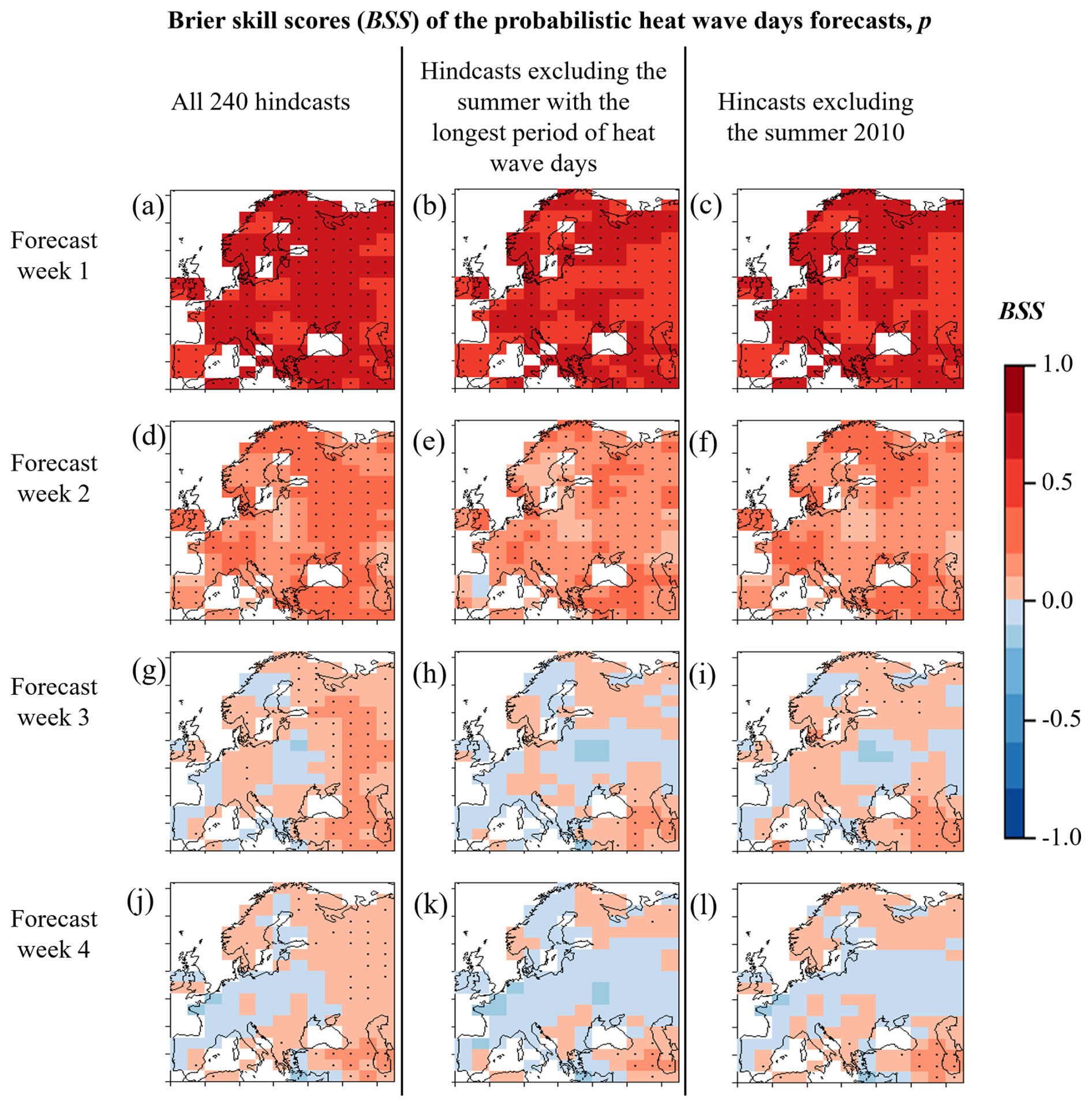
Figure 4 The Brier skill scores (BSSs) of the probabilistic heat wave day forecasts, p, during all summers 2000–2019 (first column), in hindcasts excluding the summer with the longest period of heat wave days (middle column), and in hindcasts excluding the summer of 2010 (last column). The statistical occurrence p=0.1 for heat wave days was used as the reference forecasts. The dotted areas show where the BSS is greater than zero with the false discovery rate no more than 10 %.

3.3 Verification by probability ranges

In the reliability diagram (Fig. 3b), the ERA5-based temperature data are used only as either no hot day (0) or hot day (1). Next, we conducted verification of heat wave day forecasts based on forecast probabilities falling within the ranges defined here as low: p<0.33, intermediate: $\mathrm{0.33}\le p\le \mathrm{0.66}$, and high: p>0.66; i.e., we transformed the probabilistic forecast to a categorical one. In Fig. 5, boxplots depict all the observed ERA5 temperatures (as percentiles) across different levels of p. The parts of the boxes above the 90th percentile (gray horizontal line) indicate heat wave days in the ERA5 temperature reanalysis. It is important to note that each box has a different amount of data, marked as n above each box. Due to the different amounts of hindcast data in each forecast week, as depicted in Table 1, the total amount of data differs for each lead time. The category with the most forecasts is within the low (p<0.33) range, which was also visible in Fig. 3a.

If all the heat wave day forecasts were perfect, in Fig. 5, the boxes

• for p<0.33 would be totally below the gray line, i.e., heat wave days would occur in 0 % of cases;

• for the $\mathrm{0.33}\le p\le \mathrm{0.66}$ category would be empty;

• and for p>0.66 would be totally above the gray line, i.e., heat wave days would occur in 100 % of cases.

All in all, the forecast skill improves when more of the data points in p<0.33 fall below the gray line, and those in p>0.66 are above the gray line. At a glance, forecast week 1 (Fig. 5a) appears to have good skill, while forecast week 4 (Fig. 5d) shows relatively poor skill. Further, in Fig. 5, on occasions, the forecast probability for heat wave days was low (p<0.33), heat wave days occurred in 2 % (lead time 1 week), 7 % (lead time 2 weeks), 10 % (lead time 3 weeks), or 11 % (lead time 4 weeks) of cases. Moreover, on occasions the forecast probability for heat wave days was intermediate ($\mathrm{0.33}\le p\le \mathrm{0.66}$), heat wave days occurred in 45 % (lead time 1 week), 39 % (lead time 2 weeks), 30 % (lead time 4 weeks), or 28 % (lead time 4 weeks) of cases. On occasions when the forecast probability for the heat wave days was high (p>0.66), heat wave days occurred in 86 % (lead time 1 week), 68 % (lead time 2 weeks), 67 % (lead time 4 weeks), or 38 % (lead time 4 weeks) of cases. Hence, higher probabilities (p>0.66) show that a heat wave event is more likely, but for forecast weeks 3 and 4, the forecasting signal is not very strong due to the relatively low proportion of n (amount of data) in group p>0.66. Additionally, p<0.33 provides a good indication that a heat wave is unlikely. Based on the data, the lower the p (below 0.33), the less likely a heat wave is to occur, as, e.g., on occasions when p<0.1 (no figure), heat wave days occurred only in 1 % (lead time 1 week), 4 % (lead time 2 weeks), 6 % (lead time 3 weeks), or 8 % (lead time 4 weeks) of cases.

It should be noted that Fig. 5 also shows how often forecasts were followed by a heat wave or near-heat wave conditions (e.g., temperatures exceeding the 85th percentile) in the ERA5 dataset. For instance, in situations where p>0.66, temperatures surpassing the 85th percentile (rather than the 90th percentile) occurred even in 95 % (lead time 1 week), 78 % (lead time 2 weeks), 74 % (lead time 3 weeks), or 44 % (lead time 4 weeks) of cases.

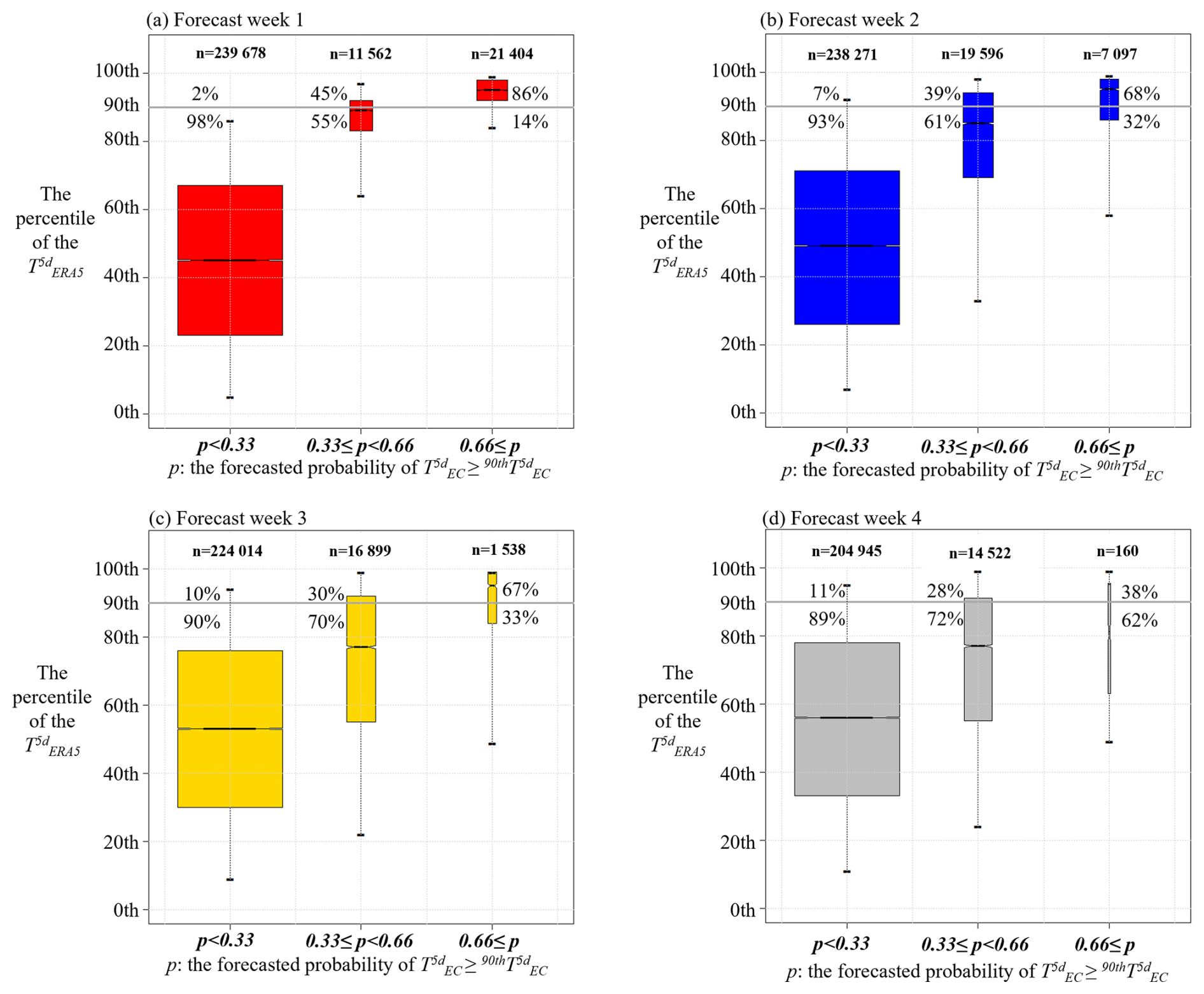
Figure 5 Boxplots of the ERA5 5 d moving average temperature over Europe in each grid point across different levels of p (the forecast probability of a heat wave day) with lead times of (a) 1 week, (b) 2 weeks, (c) 3 weeks, and (d) 4 weeks. The horizontal line dividing each box into two parts shows the median of the data, the ends of the box show the lower and upper quartiles, and the whiskers indicate the 5th and 95th percentiles of the ERA5 data in each group. The width of each box and the n written above each box indicate the number of observations in each group. The gray horizontal line indicates the 90th percentile, i.e., the threshold of a heat wave day, and the percentiles above (and below) the gray line depict the fraction of observed heat wave days (and non-heat-wave days) after the different levels of forecast probability.

3.4 Predicting the life cycle of a heat wave

Next, we shall evaluate the capacity of the probabilistic heat wave day forecasts (p) to predict the life cycle of heat waves, taking into account the forecast initialization (date) relative to the onset of the heat wave. In Fig. 6, p values are shown for days categorized according to the corresponding ERA5 data as “before the heat wave”, “during the heat wave”, and “after the heat wave”, across the entire European region at each land grid point. If there were no heat wave days during the entire summer at that grid point according to the ERA5 data, the temporal distance to the nearest heat wave day during all the heatless days of that summer was classified as “over 21 d before the heat wave”. Dashed green boxes delineate forecasts where, at the time of issuance, a heat wave in that grid point was about to begin within a week. Solid green boxes indicate forecasts where, at the time of issuance, a heat wave was ongoing in that grid point. If the forecasts were perfectly aligned with reality, p should be zero in the categories “before the heat wave” and “after the heat wave”, and in the category “during the heat wave”, p should be 1 (i.e., 100 %).

In heat wave day forecasts both 1 week in advance (Fig. 6a) and 2 weeks in advance (Fig. 6b), the forecasts show higher p for days within the heat wave than outside, especially for the forecasts in the green boxes, indicating that the heat wave was just starting or already underway when these forecasts were issued. Additionally, there is some overestimation, particularly 1–2 d before or after the heat waves, indicating slight inaccuracy in forecasting the exact day of the start and end of the heat wave. For heat wave days, forecasts are made 3 weeks in advance (Fig. 6c), higher p for days within the heat wave remains more apparent than for days outside the heat wave. Especially for the third, fourth, and fifth weeks of heat wave days, higher p values are evident compared to non-heat-wave days. These forecasts are in the green box, indicating that the heat wave was just starting or already underway when the forecast was issued. In heat wave day forecasts 4 weeks in advance (Fig. 6d), there are only slightly higher p values during the heat wave than before and after. Particularly, a small portion of the data where the fifth week of the heat wave (days 29 to 35) is in progress shows higher p. These forecasts are in the green box, indicating an ongoing heat wave when the forecast was issued.

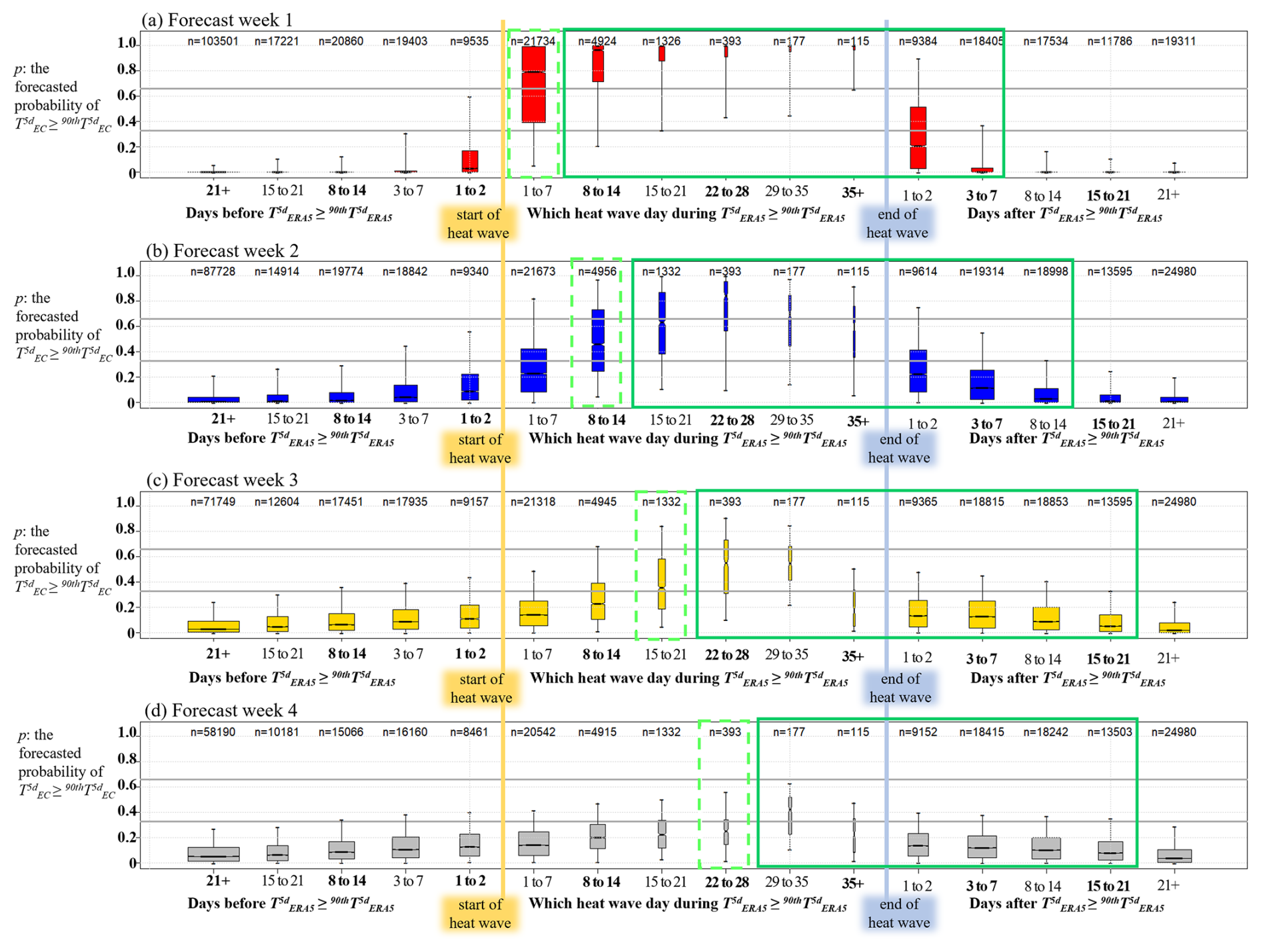
Figure 6 This figure shows the forecast probabilities of heat wave days for days that (in ERA5) were 21 to 1 d before the heat wave, the 1st to 35th heat wave day during the heat wave, and 1 to 21 d after the heat wave, with lead times of (a) 1 week, (b) 2 weeks, (c) 3 weeks, and (d) 4 weeks. Dashed green boxes indicate forecasts where, at the time of issuance, a heat wave in that grid point was about to begin within a week. Solid green boxes indicate forecasts where, at the time of issuance, a heat wave was already ongoing in that grid point. In the boxplots, a horizontal line dividing the box into two parts shows the median of the data; the ends of the box show the lower and upper quartiles, and the whiskers indicate the 5th and 95th percentiles of the data in each group. The boxplots include all forecast data across the European region at each land grid point. The width of each box and the n written above each box indicate the number of observations in each group.

We also plotted the heat wave life cycle figure without the year 2010, here shown as Fig. S1 in the Supplement. Leaving out the year 2010 removes most of the very longest heat waves, i.e., with lengths above 28 d. However, in the same way as when including the year 2010 (Fig. 6), in the forecast weeks 1–3, there is still a signal of enhanced accuracy in forecasting several-week-long heat waves at the time that the heat wave had initiated prior to the forecast issuance. Thus, the differences remain negligible.

4 Discussion

4.1 Skill of the verified probabilistic heat wave forecasts

We examined the skill of hindcasts of the ECMWF in forecasting the probability of heat wave days over Europe 1 to 4 weeks ahead. The assessed hindcasts demonstrated varying levels of accuracy across different regions, and decreasing levels with increasing forecasting lead times, which is in line with many earlier studies, e.g., Wulff and Domeisen (2019), and Pyrina and Domeisen (2023). This outcome could be seen as expected, as we employed the same forecasting model and verification region as in these previous works. However, our method for determining the probability of heat wave days was novel, providing a fresh perspective that sets our study apart from earlier research using the same model and verification region.

We investigated the impact of the longest heat waves on the forecast skill (BSS) in two ways: (i) by excluding the summer with the longest heat wave observed at each grid point and (ii) by excluding the summer of 2010, which saw a prolonged and widespread heat wave in Europe. We found that the skill in forecasting heat waves decreased when excluding the longest period of heat wave days, whether it was the 2010 heat wave or a heat wave of some other year.

Figures 6 and S1 present a novel way to evaluate the ability of probabilistic heat wave day forecasts to capture the life cycle of heat waves, taking into account the timing of forecast issuance relative to heat wave onset. This approach could be developed further by adding information about the spread of the ensemble to the figure, and it could be applied to the verification of other extended-range models' heat wave forecasts in future studies.

4.2 Potential added value of probabilistic heat wave forecasts

Currently, most heat warning systems in Europe have lead times of only a few days (Casanueva et al., 2019). However, in this study, the probabilistic heat wave day forecasts seem to have high potential in warning of heat risk in 1–2 weeks in advance, as for lead times for 1–2 weeks, there is a signal that lower probability (probabilities below 0.33) forecasts could be valuable for indicating periods when it is unlikely that a heat wave will occur, and higher-probability (probabilities above 0.66) forecasts could be valuable for indicating periods when a heat wave could occur. Further, the persistence of heat waves seems to have a higher level of predictability up to 3 weeks, offering early warning services an indication of the potential duration of an ongoing heat wave.

To the knowledge of the authors, there has been no published research on how warning lead time contributes to the effectiveness of heat-health warning systems. However, considering the short lag between heat exposure and worsening of health conditions, extending warning lead times from the current level of a few days is acknowledged to be valuable to public health, as prevention and emergency measures need to be in place and operational at the onset of a hazardous heat event (WHO, 2021). Organization of the measures, such as communication campaigns, establishing cooling centers, arrangements to protect vulnerable population groups, and ensuring adequate supply and distribution of workforce, equipment, and other resources, requires time and would benefit from receiving early warnings 1–2 weeks ahead, particularly because heat waves often occur at times when organizations and services are already short-staffed due to the summer holiday season. Longer lead time is especially important for exceptionally severe and prolonged hot periods, which challenge the functioning of society on a wider scale and may require large-scale interagency and even transboundary response. The likelihood of these types of events can be expected to increase in Europe as climate change progresses.

5 Conclusions

Our examination of ECMWF hindcasts for predicting heat wave days (periods when the local 5 d mean temperature exceeded the 90th percentile of the local summertime 5 d mean temperature distribution) of summers 2000–2019 across Europe, 1 to 4 weeks in advance, showed varying accuracy levels across forecast lead times and regions, aligning with previous research. The examined ECMWF hindcasts showed,

• in the first forecast week (1 to 7 d in advance), strong forecast skill in predicting heat wave days;

• in the second forecast week (8 to 14 d in advance), statistically significantly better skill than the reference forecast in most grid points over Europe;

• in forecast weeks 3–4 (15 to 32 d in advance), statistically significantly better skill than the reference forecast only in some grid points across southeastern Europe; and

• in forecast weeks 1–3, enhanced accuracy in forecasting several-week-long heat waves at the time that the heat wave had already started.

These findings underscore the potential of ECMWF's heat wave day forecasts to serve as early warnings for impending heat risks 1–2 weeks in advance. Notably, the higher-than-average predictability for intense and prolonged heat waves (at the time they have already started) offers the potential for early warnings even at a 3 week lead time. However, it is crucial to highlight the known uncertainty in the 3 week lead time forecast. Building on these insights, future research could investigate at which stage of the heat wave development extended-range weather forecast models in general, not only the specific model system considered here, begin to predict heat wave occurrence, potentially enhancing early warning capabilities.