Using a convection-permitting climate model to assess wine grape productivity: two case studies in Italy

The article explores the potential use of climate models to reproduce wine grape productivity at a local scale in Italy. To this end, both single and multiple regression approaches are used to link productivity data provided by two Italian wine consortia with bioclimatic indices. Temperature- and precipitation-based bioclimatic indices are computed using the observational dataset E-OBS, the high-resolution climate reanalysis product SPHERA, the regional climate model CNRM-ALADIN, and the kilometer-scale convection-permitting climate model CNRM-AROME. The multiple regression method outperforms the single regression systematically, enhancing the ability of bioclimatic indices to explain productivity variability. The results show that productivity is strongly tied to temperature-based bioclimatic indices in the area of the Consorzio per la tutela del Franciacorta in northern Italy, while for the Consorzio del Vino Nobile di Montepulciano area in central Italy both temperature- and precipitation-based indices are relevant. Climate models, providing similar results as E-OBS and SPHERA, appear to be a useful tool to explain productivity variance. In particular, the added value of convection-permitting resolution is evident when precipitation-based indices are considered. This assessment shows windows of opportunity for using climate models, especially at a convection-permitting scale, to investigate future climate change impact on wine production.

1 Introduction

Viticulture is tied to climate, which influences the suitability of an area, as well as yield and quality of wine grapes. The wine industry has a significant socioeconomic influence and is a key agricultural sector in Italy. In 2022, Italy was the world's leading wine producer (49.8 million hectoliters) and the second-largest wine exporter, with a value of EUR 7.8 billion (OIV, 2023). Over the coming decades, the wine sector is expected to be affected by climate change, especially in Italy, which is part of the Mediterranean climatic hotspot (Giorgi, 2006; Tuel and Eltahir, 2020), where the impact of climate change is expected to be more severe than the global average. In this context, many studies have investigated the impact of rising temperatures and changing rainfall patterns on grape growth (Bagagiolo et al., 2021; Bernetti et al., 2012; Gentilucci, 2020; Roehrdanz and Hannah, 2016; Sacchelli et al., 2017; Santillán et al., 2020). Since temperature is the primary driver for the phenological phases (Fraga et al., 2016), a warmer climate may lead to a shorter growing cycle and an earlier onset of phenological phases, which would increase frost-related risk (Lamichhane, 2021; Trought et al., 1999). In fact, budburst is the most vulnerable phase to frost in the vine growing cycle, and an earlier budburst in spring would increase the exposure of the vine to late frost events. Furthermore, climate conditions typical of traditional wine-producing regions, such as Douro in Portugal, La Rioja in Spain, Bordeaux in France, and Tuscany in Italy, are expected to shift northwards or to higher altitude, and this modification in viticulture suitability may consequently cause a decline in production (Adão et al., 2023; Rafique et al., 2023; Sgubin et al., 2023; Tóth and Végvári, 2016).

A common tool to investigate the impact of climate variability and change on the wine sector is the use of bioclimatic indices, defined from climate variables for specific plants and crops (Badr et al., 2018; Chou et al., 2023; Gaitán and Pino-Otín, 2023). A set of bioclimatic indices, based on temperature and heat accumulation (OIV, 2015), was proposed by the International Organisation of Vine and Wine (OIV), while precipitation-based indices were computed by Badr et al. (2018) considering the research of Blanco-Ward et al. (2007). Bioclimatic indices are commonly used to assess a region's suitability for viticulture or zoning purposes, as well as in relation to phenology, harvest date, and alcohol concentration (Dalla Marta et al., 2010; Koufos et al., 2014; Sánchez et al., 2019; Teslić, 2018). A novel application linking bioclimatic indices directly to wine grape productivity data in Italy was proposed by Massano et al. (2023) at the regional level.

In Italy the vineyards are planted in extremely different areas, from the coasts to the hills, in some cases also at considerable altitude (Tarolli et al., 2023). The wine production system is complex and fragmented, including both small farms and large companies. To valorize the designation of origin and guarantee a defined level of quality (Gori and Alampi Sottini, 2014; Ugaglia et al., 2019), producers are organized in wine consortia (Consorzi di Tutela) according to the EU and national regulations, i.e., regulation (EU) no. 1308/2013. To address this fragmentation and account for the typicity of the wine business (Agnoli et al., 2023; Spielmann and Charters, 2013), yield data from wine consortia and high-resolution climate data are of prominent importance for local-scale impact studies and thus for effective adaptation strategies.

In the context of impact studies at a local scale, requiring high-resolution climatic data, the use of kilometer-scale convection-permitting models (CPMs) is increasing (Bamba et al., 2023; Le Roy et al., 2021; Tradowsky et al., 2023). Due to their high spatial resolution (less than 4 km), CPMs can represent convection explicitly, without using the parameterization of deep convection, and thus reduce the model uncertainty (Fosser et al., 2024). Compared to coarser-resolution regional climate models (RCMs), CPMs more realistically represent hourly rainfall intensity, the diurnal cycle of precipitation, and extremes and are thus considered more reliable in terms of climate projections of precipitation (Ban et al., 2021; Brisson et al., 2016; Coppola et al., 2020; Fosser et al., 2020; Kendon et al., 2017; Pichelli et al., 2021). The advantages of CPMs versus RCMs have been also explored in the assessment of the impact of climate change on agriculture and crop production (Agyeman et al., 2023; Berthou et al., 2019; Chapman et al., 2020, 2023). Nevertheless, no prior studies have employed CPMs to examine the influence of climate variability and change on viticulture.

The present study presents a novel approach to estimate wine grape productivity at the local scale by using a CPM, showing windows of opportunity for the use of CPMs in the context of ongoing and future climate change. The impacts of climate variability on wine grape productivity are investigated by relating temperature- and precipitation-based bioclimatic indices to wine productivity data provided by two wine consortia in northern and central Italy. The CPM performance is validated against climate observations and a kilometer-scale reanalysis product. Furthermore, the added value of the higher resolution is assessed by comparing the CPM to an RCM simulation. Single and multiple regression approaches are used to determine to what extent bioclimatic indices can explain changes in wine grape productivity at a local scale. The multiple regression approach accounts for the potential interplay between the bioclimatic indices, potentially increasing the portion of total productivity variability explained by the individual indices, as found by Massano et al. (2023).

2 Data and methods

2.1 Wine grape productivity data

Wine grape yield data, as well as the hectares of vines, are collected from two wine consortia in Italy: the Consorzio per la tutela del Franciacorta (FRA) and the Consorzio Del Vino Nobile di Montepulciano (MON). The first one lies in Franciacorta, a small (200 km²) wine-growing region in Lombardia (LOM), northern Italy, mostly known for sparkling wine (Fig. 1). The area is characterized by a humid subtropical climate according to the Koppen classification (Costantini et al., 2013). The Iseo lake, located at the northern border of this region, is the sixth-largest lake in Italy and tempers the typical heat of the plain in summer, while in winter it protects the vineyards from the freezing air arriving from the north (Leoni et al., 2019). The consortium was born in 1990 as a result of the endeavor of local producers that felt the need to preserve the original production method of Franciacorta wine. Today the consortium is composed of 200 winemakers and preserves three designations: Sebino IGT (Typical Geographical Indication), Franciacorta DOCG (Denomination of Controlled and Guaranteed Origin), and Curtefranca DOC (Denomination of Controlled Origin), known as Terre di Franciacorta before 2011 (https://franciacorta.wine/en/, last access: 2 March 2024). This analysis focuses on the designations of Franciacorta DOCG and Curtefranca DOC available from 1997 to 2019 (23 years), discarding Sebino IGT, for which data are only available for a limited period.

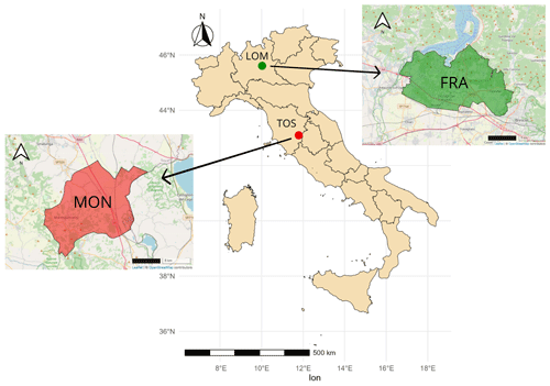
Figure 1 Map of Italy highlighting in green the area of the Franciacorta consortium (FRA) in the Lombardia (LOM) region and in red the area of the Consorzio del Vino Nobile di Montepulciano (MON) in the Toscana (TOS) region (base layer: © OpenStreetMap contributors 2019. Distributed under the Open Data Commons Open Database License (ODbL) v1.0.).

The Consorzio del Vino Nobile di Montepulciano (MON) (https://www.consorziovinonobile.it/, last access: 2 March 2024) is located within the Montepulciano territory in Toscana (TOS) region in the center of Italy (Fig. 1). The area is characterized by a Mediterranean climate with a hot and dry summer and mild and rainy winters (Costantini et al., 2013). The consortium preserves three designations, namely Vino Nobile di Montepulciano DOCG, Rosso di Montepulciano DOC, and Vin Santo di Montepulciano DOC. The study focuses on the first two designations that have the longest time series covering 31 years between 1989 and 2019.

For each wine designation, the FRA consortium directly reports the quantity of grapes harvested in quintals (q), while MON indicates the hectoliters of wine produced (hL) and the maximum percentage of grape yield convertible into wine (70 %). For the analysis, the hectoliters are converted into quintals using the maximum percentage allowed, and then the productivity (q ha⁻¹) is calculated by dividing the quintals of grapes by the vineyard area.

To assess the consistency of productivity data between local and regional scales, the productivity at the local scales (FRA and MON) is compared with productivity at a regional scale provided by the Italian National Institute of Statistics (ISTAT). ISTAT provides data of harvested wine grape (in quintals) and vintage area (in hectares) from 1980 onwards. However, the data are not homogenous over time in terms of spatial aggregation. Wine grape productivity data are available at the provincial level between 1980 and 1993 and from 2006 to 2019, at the regional level between 1994 and 2000, and at the national scale from 2000 to 2005. Following Massano et al. (2023), the data were aggregated at a regional level for the Lombardia (LOM) and Toscana (TOS) regions, where the FRA and MON consortia are respectively located, for the period 1980–2019, with a 6-year gap between 2000 and 2005. Considering the overlapping periods between ISTAT and consortia time series, it is found that the regional and local productivity data are significantly correlated ($p\le =\mathrm{0.05}$) for both FRA and MON (Table A1). In addition, the application of a Welch's t test, designed to assess whether two samples are extracted from the same population, proves that the productivity distributions of both consortia are consistent with the respective regional productivity distributions (Table A1 and Fig. A1).

2.2 Climate observations and reanalysis data

The observational dataset used is E-OBS, a gridded daily dataset covering Europe from January 1950 to the present day. E-OBS is constructed using data from the meteorological stations provided by the European National Meteorological and Hydrological Services or other data-holding institutions (Photiadou et al., 2017; Van Der Schrier et al., 2013). The analysis is based on the latest available version (v28) at 0.1° (∼11 km). Although the E-OBS database is frequently used to validate climate models (Christensen et al., 2008; Jaeger and Seneviratne, 2011; Lorenz and Jacob, 2010; Retalis et al., 2016), some studies have pointed out some limitations in the E-OBS representation of precipitation and temperature, mainly due to the inhomogeneity of the station network used for interpolation (Kyselý and Plavcová, 2010; Liakopoulou and Mavromatis, 2023; Van Der Schrier et al., 2013).

In addition to observations, the analysis uses a high-resolution convection-permitting reanalysis product, called SPHERA (High rEsolution ReAnalysis over Italy; Cerenzia et al., 2022; Giordani et al., 2023), produced by ARPAE-SIMC (Agency for Environmental Protection of the Emilia Romagna Region, Italy). Based on the non-hydrostatic limited-area model COSMO (Baldauf et al., 2011; Schättler et al., 2018), SPHERA dynamically downscales the global reanalysis ERA5 (Hersbach et al., 2020) boundary condition, updated every hour, in a sequence of 24 h long integrations. Being a reanalysis product, SPHERA assimilates in situ observations using a continuous nudging approach based on the Newtonian relaxation principle (Stauffer and Seaman, 1990). The quality-checked observational data nudged in SPHERA are wind speed components, pressure, air humidity, and temperature (excluding 2 m temperature) derived from the ECMWF catalogue, i.e., SYNOP, SHIP, TEMP, PILOT, and AIREP. More details on the SPHERA configuration can be found in Cerenzia et al. (2022). This new reanalysis product covers Italy at a horizontal resolution of 2.2 km with a temporal coverage of 26 years (1995–2020). When validated against independent rain gauge observations, SPHERA showed an improved representation of the precipitation field at both daily and hourly scales compared to its driver, i.e., ERA5 (Giordani et al., 2023). The performance of SPHERA demonstrates that it can be a valuable resource for improving climate monitoring by providing insights into regional climate change impacts (Giordani et al., 2023). The SPHERA data, provided at hourly time steps, have been aggregated at the daily timescale for the purpose of this study.

In this study, the E-OBS dataset and SPHERA reanalysis are both employed as a reference. This strategy enhances the validation process and evaluates the potential of a reanalysis product to serve as an alternative to observations for the validation of climate models as well as for viticulture studies.

2.3 Climate model data

The French Centre National de Recherches Météorologiques (CNRM) provides two climate simulations spanning the period 2000–2018. The first simulation, covering the Med-CORDEX domain (Ruti et al., 2016) at 12.5 km resolution, is performed with the RCM CNRM-ALADIN (Nabat et al., 2020), the limited-area version of ARPEGE-Climate global model, driven every 6 h by the ERA-Interim (80 km) reanalysis (Dee et al., 2011). The second one is performed with the CPM CNRM-AROME, driven by the CNRM-ALADIN simulation every hour, and covers the pan-Alpine domain defined within the CORDEX FPS on convection program with a resolution of 2.5 km (Coppola et al., 2020; Lucas-Picher et al., 2024). In contrast to any reanalysis dataset (e.g., SPHERA), climate models do not assimilate observations. This has the disadvantage of usually leading to larger biases than reanalysis (at least for variables which are assimilated in the reanalysis), but the advantage is that they can be used for climate projections. The main difference between CNRM-ALADIN and CNRM-AROME resides in the parameterization of deep convection, which may be a source of errors and uncertainty (e.g., Prein et al., 2015), active in the former and switched off in the latter. In addition, CNRM-AROME, being a kilometer-scale model, allows a more accurate representation of surface and orographic features. Both models have been extensively evaluated (e.g., Ban et al., 2021; Coppola et al., 2020; Daniel et al., 2019; Fumière et al., 2020; Nabat et al., 2020; Pichelli et al., 2021). In particular, Caillaud et al. (2021) found that CNRM-AROME, besides an underestimation of the highest intensities, realistically represents autumn extreme precipitation at both daily and hourly timescale in terms of location, intensity, frequency, and interannual variability, while CNRM-ALADIN fails to do so. Both CNRM-ALADIN and CNRM-AROME (hereafter simply called RCM and CPM, respectively ) provide hourly outputs, which are aggregated at the daily timescale for the purpose of this study.

2.4 Validation of climate simulations

In this work, temperature and precipitation data from the observational dataset E-OBS, the climate reanalysis product SPHERA, and the climate model simulations, at regional (RCM) and convection-permitting scale (CPM), are used for the calculation of a set of bioclimatic indices described in the next section. The analysis focuses on the 19 years from 2000 to 2018, which is the longest period available for RCM and CPM simulations that is shared with E-OBS, SPHERA climate data, and FRA and MON productivity data. To compare datasets with different horizontal resolutions on equal terms (Berg et al., 2013), observations, reanalysis, and model simulations are conservatively remapped on a common grid, i.e., the E-OBS regular grid at ∼11 km, the coarsest among all. Tests performed to assess the impact of upscaling SPHERA and CPM at a coarser resolution showed no significant changes in the results (not shown).

Then, the climatic variables (i.e., P: precipitation; TM: mean temperature, TX: max temperature; TN: min temperature) are retained on all available grid cells within the areas of interest (LOM and TOS). Subsequently, the consortium territory is cropped using the respective shape files of FRA and MON. Finally, the spatial average is calculated by weighting the contribution of each grid cell according to the percentage of the cell falling within the consortium territory. The shape file of the FRA consortium's territory is provided directly by the consortium's technical office, while the shape file for MON is created by selecting the municipality listed in the appellation regulation for the relevant denominations (i.e., Montepulciano municipality).

The precipitation and temperature time series of the climate simulations are analyzed against the observational datasets (i.e., E-OBS and SPHERA) to evaluate the biases in the climatic conditions in the region of interest prior to examining the bioclimatic indices. In particular, the CPM performance is evaluated for the period 2000–2018 against both SPHERA and E-OBS and compared to the RCM. In this study, the new SPHERA reanalysis product is used as a reference dataset together with the E-OBS dataset, which is already widely used for model validation (Kyselý and Plavcová, 2010). The comparison between climate model simulations and the reference datasets is carried out by computing the Spearman correlation, the root mean square error (RMSE), and normalized root mean square error (NRMSE) with respect to the range of values, i.e., the maximum value of the variable considered (y_max) minus the minimum value (y_min), for the reference datasets (SPHERA and E-OBS). In particular, the Spearman correlation coefficient is used to assess the ability of the climate models to reproduce the climate variability of the reference datasets, while RMSE and NRMSE provide a measure of the climate models biases. Moreover, the statistical significance of the model biases is assessed by applying a Welch's two-tailed t test (Welch, 1938) with a 95 % level of confidence.

2.5 Bioclimatic indices

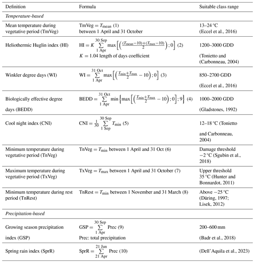
This study considers 10 bioclimatic indices (summarized in Table 1), computed following the same methodology previously described for the climate variable. Eight of them, recommended by the International Organisation of Vine and Wine (OIV), are based on temperature and heat accumulation, while the remaining two are based on rainfall accumulation.

Table 1 Acronyms and formulas of the bioclimatic indices used.

The temperature-based indicators are the following.

1. The daily mean temperature during the vegetative period (TmVeg) is calculated between 1 April and 31 October (Jones et al., 2005). Temperature in spring plays a key role in determining the timing of phenological events, as underlined by Malheiro et al. (2013). In general, higher TmVeg leads to an anticipation of the phenological phases, while TmVeg values above 24 °C or below 12 °C are considered unfavorable to wine growing (Eccel et al., 2016).

2. The heliothermic Huglin index (HI) is calculated by summing, when positive, the average between the mean and the maximum temperature in relation to the baseline temperature of 10 °C, i.e., the physiological threshold for the start of the vine growth cycle (Huglin, 1978; Teslić, 2018), over the period from 1 April to 30 September corrected by a coefficient of day duration. The HI index is tied to vine growing and grape sugar concentration, with higher HI leading to an increased vine vigor and higher sugar content in the grapes. According to Tonietto and Carbonneau (2004), a climate with a heat index (HI) of more than 3000 degree days (GDD) is classified as “very warm”, while fewer than 1200 degree days is classified as “too cold”. Both of these situations are associated with plant stress and thus lead to a production reduction.

3. Winkler degree days (WI) provide a measure of heat accumulation during the growing season and are the sum of daily mean temperatures above 10 °C from 1 April to 31 October (Amerine and Winkler, 1944; Piña-Rey et al., 2020). Similarly to HI, the WI index is linked to the rate of growth of the vines and the development of the fruits, with values between 850 and 2700 degree days being optimal for wine production (Eccel et al., 2016).

4. Biologically effective degree days (BEDDs) represent the sum of daily mean temperatures in the range between 10 and 19 °C from 1 April to 31 October. The BEDD index uses the same baseline temperature (10 °C) as WI and HI indices but also takes into consideration that vine growth is unlikely to occur above the upper temperature threshold of 19 °C (Anderson et al., 2012; Gladstones, 1992). Like the previous temperature-based indices, values of BEDD that are too high (above 2000° per day) or too low (below 1000° per day) can potentially reduce productivity.

5. The cool night index (CNI) is defined as the average of minimum air temperatures during the month of September. Low minimum temperatures in September increase the polyphenolics in the grapes and are beneficial for the overall quality of the harvest (Tonietto and Carbonneau, 2004). Although CNI is more related to grape quality than quantity, Massano et al. (2023) found that this index can help explain changes in productivity, especially when used in combination with other bioclimatic indices.

6. The minimum temperature during the vegetative period (TnVeg) is the minimum temperature recorded during the vegetative period (1 April to 31 October). This index is important to assess whether the vines are exposed to low temperature or even to spring frosts that pose a significant risk to viticultural practices and production. The damage threshold is fixed at −2 °C (Sgubin et al., 2018).

7. The maximum temperature during the vegetative period (TxVeg) is the maximum temperature recorded during the vegetative period. This index is useful for assessing the occurrence and the severity of summer hot-spells that can damage to vineyard, thus reducing the wine productivity (Cabré and Nuñez, 2020). The heat stress threshold is set at 35 °C, above which physiological damage to the vines is expected (Hunter and Bonnardot, 2011).

8. The minimum temperature during the rest period (TnRest) is defined as the minimum temperature during the rest period, i.e., 1 November to 31 March. This index is used to determine winter severity. Grapevines can tolerate temperatures as low as −25 °C (Düring, 1997; Lisek, 2012), although damage can already occur at −15 °C (Eccel et al., 2016)

The indices based on precipitation are the following.

1. The growing season precipitation index (GSP) is defined as rainfall accumulated from 1 April to 30 September and is used to assess the water stress for non-irrigated grapevines (Blanco-Ward et al., 2007; Piña-Rey et al., 2020), as in Italy where irrigation is only allowed in extreme cases (e.g., long drought periods).

2. The spring rain index (SprR) measures the amount of rain accumulated between 21 April and 21 June (Marcos-Matamoros et al., 2020). This indicator of spring wetness can be related to production. In fact, while dry springs can delay vegetation growth, wet ones can increase plant vigor but also lead to a higher risk of fungal diseases (Dell'Aquila et al., 2023).

The bioclimatic indices computed using climate simulations (RCM and CPM) are analyzed against the observational datasets (E-OBS and SPHERA) following the same methodology described for the climatic variables (i.e., P: precipitation; TM: mean temperature, TX: max temperature; TN: min temperature).

2.6 Trend analysis

A trend analysis for both the climatic variables and the bioclimatic indices is performed to assess the evolution of the climatic condition in FRA and MON in the period 2000–2018; the same analysis is also carried out for productivity data. The presence and the magnitude of trends are respectively determined using the nonparametric Mann–Kendall test and the Sen's slope method, with a significance level of 95 % (Hanif et al., 2022; Mann, 1945). The Sen's slope estimator calculates the rate of change over time of a variable by taking the median of the slopes of all linear regressions between points pairs (Aswad et al., 2020). The assessment of possible trends aims to investigate whether the long-term component of variability may be dominant over the interannual component.

2.7 Single and multiple regression approach

The Spearman correlation coefficient between each bioclimatic index and the wine grape productivity is calculated for both consortia areas, and the threshold for statistical significance is set to 95 %. This analysis aims at assessing the fraction of wine grape productivity variability explained by the bioclimatic indices and the ability of climate models to represent this relationship compared to the observational datasets.

Furthermore, a multiple regression (MR) approach is applied to determine whether a linear combination of indices can enhance the total productivity variability explained by the bioclimatic indices (Massano et al., 2023). The best-subset selection approach, implemented by James et al. (2013), is used to optimize the prediction of productivity, as in Massano et al. (2023). This approach seeks the subset of predictors, i.e., the bioclimatic indices in this case, that most accurately predicts the predictand, i.e., the productivity, by examining all feasible predictor combinations and thus selecting the one minimizing the error in the prediction. This is achieved by utilizing the k-fold cross-validation method. The k-fold cross-validation method is employed to identify the optimal model (Kassambara, 2018). This method performs cross-validation by randomly dividing the data into k subsets of approximately equal size, with k typically set to 5 or 10 (here k=5 is used). One of the folds serves as a test set and the remaining as a training set. This process is repeated k times, whereby varying groups of data are utilized as training or testing sets. Subsequently, the mean squared error is computed. The average of the mean squared errors of all iterations is the model prediction error (CV – cross-validation error) (James et al., 2021; Kuhn and Johnson, 2013; Wassennan, 2004). The performance of the multiple regression model is assessed by the adjusted R² coefficient of determination (Adj R²), while the p value is used to determine statistical significance at the 95 % level. The so-optimized MR model (productivity = a₁ ⋅ index₁ + a₂ ⋅ index2 + a₃ ⋅ index₃ + …, with index_n indicating the selected bioclimatic index) is then used to predict the productivity, and the Pearson correlation between predicted and observed productivity is calculated. Following Massano et al. (2023), the comparison between the SR and MR methods is performed in terms of the productivity variance explained by the prediction, estimated by computing the coefficient of determination, i.e., the square of the correlation coefficient.

3 Results

3.1 Validation of the climate simulations

Prior to the computation of the bioclimatic indices, the precipitation and temperature fields in both consortia (FRA and MON) are analyzed to assess the potential biases, which could impact the temperature- and precipitation-based bioclimatic indices. Figure 2 for FRA and Fig. 3 for MON show the precipitation (P) and temperature (TM: mean temperature, TX: max temperature, and TN: min temperature) time series of E-OBS, SPHERA, RCM, and CPM for the period 2000–2018. In general, both RCM and CPM reproduce SPHERA temporal variability well, as also confirmed by the high and significant correlations for all the climate variables in both consortia (Table A2). Nevertheless, both climate models tend to overestimate mean and maximum temperature while underestimating minimum temperature, as reflected by the statistical differences in mean values (Table A3). Both climate models, especially the RCM, underestimate precipitation in FRA, while the CPM tends to overestimate it in MON. Precipitation in MON is also slightly overestimated by the RCM. In FRA, RCM is closer to E-OBS mean values than CPM (Table A3). However, in MON, E-OBS minimum temperature time series shows a strong decrease of almost 2 °C between 2015 and 2018 (Fig. 3), which is not observed in any models or SPHERA. Further investigations revealed that this temperature decline is observed throughout the entire TOS and is inconsistent with other observational records (not shown). This E-OBS misrepresentation of the temperature field has a subsequent effect on the mean and minimum temperature time series (Fig. 3), as well as the temporal correlations (Table A2), and is likely to be reflected in the temperature-based bioclimatic indices in the TOS region and at the local scale in MON.

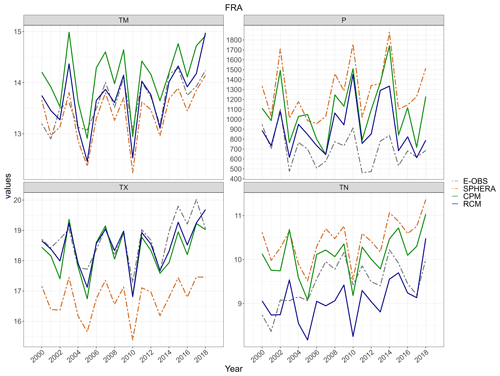
Figure 2 Time series of mean (TM), maximum temperature (TX), minimum (TN) temperature, and precipitation (P) over the FRA area for E-OBS (dashed gray), SPHERA (dashed red), RCM (solid blue), and CPM (solid green) for the period 2000–2018. All the time series are based on data remapped on the E-OBS grid (∼11 km).

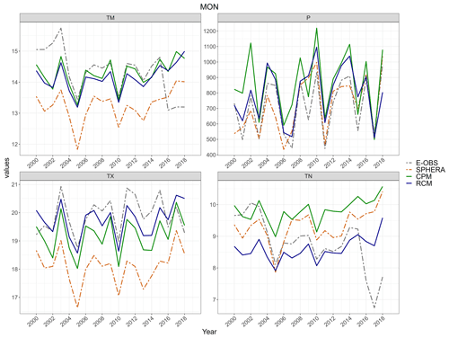
Figure 3 Time series of mean (TM), maximum temperature (TX), minimum (TN) temperature, and precipitation (P) over the MON area for E-OBS (dashed gray), SPHERA (dashed red), RCM (solid blue), and CPM (solid green) for the period 2000–2018. All the time series are based on data remapped on the E-OBS grid (∼11 km).

The time series of the bioclimatic indices considered are shown in Figs. 4 and 5. All the bioclimatic indices show very high and significant temporal correlation between SPHERA and both RCM and CPM in both consortia, as shown by Figs. 6a and 7a. The correlations are particularly high (i.e., above 0.8) for all temperature-based bioclimatic indices except for TnVeg and TxVeg, which appear more sensitive to the biases in minimum and maximum temperature (Figs. 2 and 3). The correlations with precipitation-based indices are still high (between 0.64 and 0.91) for SprR but drop for GSP in MON for both CPM and RCM. Similar conclusion can be drawn for the comparison of the climate models with E-OBS in FRA, while in MON four temperature-based indices (i.e., BEDD, WI, TnVeg, CNI) are not significantly correlated, likely due to the low correlations in mean and minimum temperature (Table A2). The correlations, especially with SPHERA, tend to be slightly higher for the CPM than for the RCM for most indices, despite the higher NRMSE in the CPM (Figs. 6b and 7b). The strong correlation between SPHERA and climate simulations (Figs. 6a and 7a) indicates that RCM and CPM reproduce the same temporal variability in the bioclimatic indices as SPHERA, despite the statistical differences in mean values (Table A4). The same conclusion is also valid for the comparison of RCM and CPM to E-OBS, at least for FRA. This analysis suggests that both CPM and RCM could be a valid alternative to the reanalysis product to investigate the impact of climate on viticulture, despite the biases affecting the climate simulations. In addition, the reanalysis allows a more realistic representation of bioclimatic indices, overcoming the pitfalls of the observational dataset E-OBS in TOS.

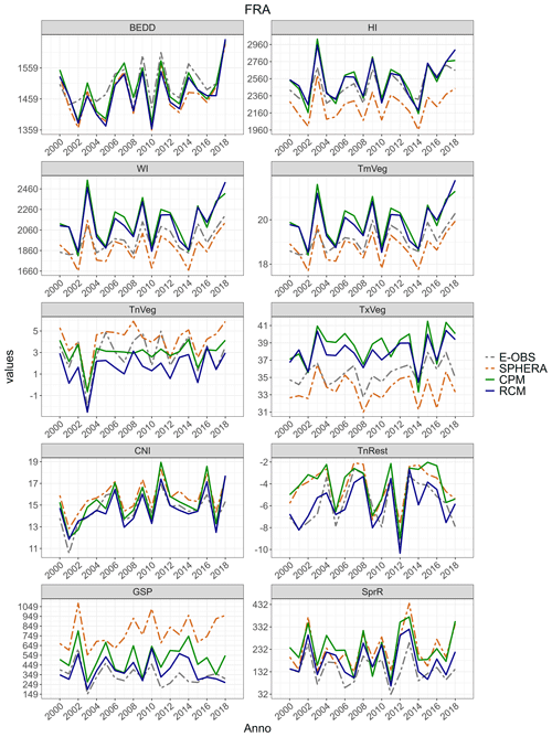
Figure 4 Time series of the bioclimatic indices considered: biologically effective degree days (BEDD), heliothermic Huglin index (HI), Winkler index (WI), daily mean temperature during the vegetative period (TmVeg), minimum temperature during the vegetative period (TnVeg), maximum temperature during the vegetative period (TxVeg), cool night index (CNI), minimum temperature during the rest period (TnRest), growing season precipitation index (GSP), and spring rain index (SprR) over the FRA area for E-OBS (dashed gray), SPHERA (dashed red), RCM (solid blue), and CPM (solid green) for the period 2000–2018. All the time series are based on data remapped on the E-OBS grid (∼11 km).

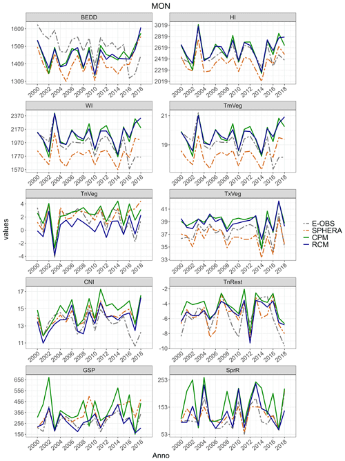
Figure 5 Time series of the bioclimatic indices considered: biologically effective degree days (BEDD), heliothermic Huglin index (HI), Winkler index (WI), daily mean temperature during the vegetative period (TmVeg), minimum temperature during the vegetative period (TnVeg), maximum temperature during the vegetative period (TxVeg), cool night index (CNI), minimum temperature during the rest period (TnRest), growing season precipitation index (GSP), and spring rain index (SprR) over the MON area for E-OBS (dashed gray), SPHERA (dashed red), RCM (solid blue), and CPM (solid green) for the period 2000–2018. All the time series are based on data remapped on the E-OBS grid (∼11 km).

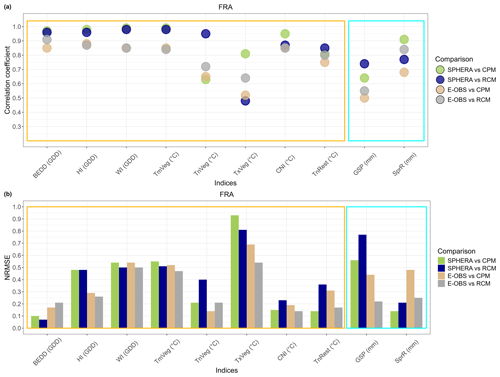
Figure 6 For the FRA area, the figure shows (a) the Spearman correlation coefficient of the indices' time series and (b) the normalized root mean square error (NRMSE) with respect to the range of values (y_max–y_min) of the reference (SPHERA and E-OBS). Colors represent the different comparisons performed and full-colored dots in panel (a) indicate a statistically significant result (p≥0.05).

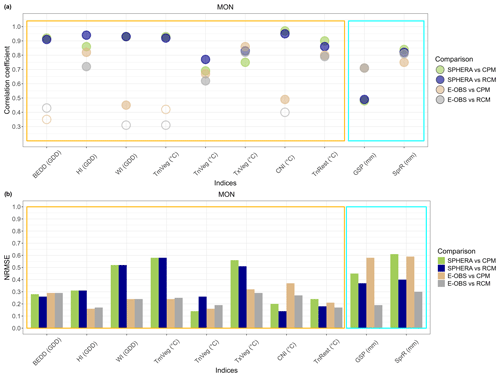
Figure 7 For the MON area, the figure shows (a) the Spearman correlation coefficient of the indices' time series and (b) the normalized root mean square error (NRMSE) with respect to the range of values (y_max–y_min) of the reference (SPHERA and E-OBS). Colors represent the different comparisons performed and full-colored dots in panel (a) indicate a statistically significant result (p≥0.05).

3.2 Bioclimatic index control on wine grape productivity

3.2.1 Single regression analysis

A Spearman correlation analysis is performed to investigate the relation between the different bioclimatic indices and wine grape productivity and to consequently determine the amount of total productivity variability (interannual and long-term) explained by these indices.

In FRA, the correlation coefficients are similar between climate simulations, observations, and reanalysis for some of the temperature-based indices, while they diverge and are not significant for the precipitation-based ones (Fig. 8). Statistically significant cases are CNI with climate model simulations, SPHERA, and E-OBS and the BEDD index only when RCM and E-OBS are used. Nevertheless, some of these bioclimatic indices (i.e., BEDD for E-OBS and CNI for CPM) as well as the FRA productivity show significant trends (Tables A5 and A7); thus, these significant correlations may depend on the long-term variability (i.e., the trend) rather than on the interannual variability. The RCM also presents a statistically significant and positive correlation between productivity and TnRest, which does not show a trend over the period 2000–2018, suggesting that TnRest variability has a role in controlling productivity at the interannual timescale. The statistically significant coefficients are all positive, indicating a positive effect on productivity of BEDD, CNI, and TnRest.

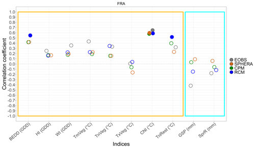
Figure 8 Spearman correlation coefficients between bioclimatic indices and wine grape productivity in FRA. Full-colored circles indicate significant correlations ($p\le =\mathrm{0.05}$).

In MON, the correlations between productivity and bioclimatic indices are similar across all the datasets for BEDD, HI, WI, and TmVeg but show greater variation for all other temperature-based and precipitation-based indices (Fig. 9). Significant results are found for TnVeg, only using CPM, and for TxVeg in all datasets. It is notable that TxVeg displays a negative correlation, indicating that extreme temperatures during the growing period have a detrimental effect on production. This aligns with winemaker expectations and is partially supported by the results from FRA (Fig. 8), despite not being statistically significant. Both TnVeg and TxVeg indices show a significant positive trend for most datasets (Table A6), which suggests that productivity is more sensitive to the long-term variability. Productivity data do not show any trend in MON (Table A7).

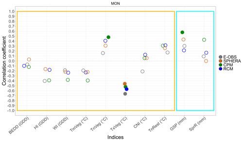
Figure 9 Spearman correlations between bioclimatic indices and wine grape productivity in MON. Full-colored circles indicate significant correlations ($p\le =\mathrm{0.05}$).

Only the CPM simulation shows significant correlation for the precipitation-based index GSP. This could be linked to the more realistic representation of the precipitation field (Prein et al., 2015), although positive correlations with GSP are not expected, as an excessively wet season is usually detrimental to production. Thus, it is possible that other factors influence this correlation, such as specific viticultural practices or vintage management (Priori et al., 2019). For example, harvesting immediately after rainfall may result in the collection of larger grapes, thus increasing the productivity. Additionally, specific trimming techniques can improve the ventilation between the branches, reducing the risk of mold and fungus and thus limiting the negative impact of precipitation on the harvest (Evers et al., 2010).

3.2.2 Multiple regression analysis

A multiple regression (MR) analysis is carried out and compared with the single regression (SR) approach to see if considering a linear combination of bioclimatic indices increases the proportion of productivity variability explained by the indices.

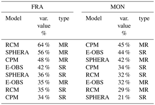
Table 2 shows the results of the MR model, highlighting the selected bioclimatic indices and the variance explained in comparison with the SR method, for each case in both FRA and MON. The authors highlight that, even when the MR selects just one index, this can differ from the single regression due to the correlation method chosen. The MR confirms that the temperature-based bioclimatic indices are more relevant than precipitation-based ones in explaining productivity variability, especially in FRA, where only for the RCM is the GSP selected as a predictor. The selection of GSP for the RCM is unexpected. Indeed, although GSP from the RCM shows high and significant correlations with both the CPM (not shown) and SPHERA (Fig. 6), it is not selected by the MR model for the CPM and SPHERA. The comparison between the standardized beta coefficients (Dodge, 2008) of the MR model for RCM in FRA shows that GSP has the least impact on the explained variance of the observed productivity, suggesting that the selection of GSP for the RCM only might be an artifact of the statistical model. In MON, precipitation-based indices are selected as predictors in the MR model when using the CPM simulation and SPHERA reanalysis, confirming the relatively higher importance of precipitation for productivity in this area compared to FRA. Thus, for MON, the improved representation of the precipitation field at a convection-permitting scale could be a relevant factor, since in other datasets at coarser resolution (i.e., E-OBS and RCM) precipitation-based indices are excluded by the MR. To improve the understanding of this aspect and clarify the relative importance of the precipitation-based indices for the two study areas, the same methodology employed here could be applied to other climatic datasets derived from different convection-permitting models.

Table 2 Donut chart indicating, for E-OBS, SPHERA, CPM, and RCM, the best-performing index for the single regression (SR) and the indices included in the multiple regression model (MR), as well as the percentage of variance explained by each statistical model (center of the donut), in FRA and MON. The percentage of variance is calculated as the squared coefficient of determination of the Spearman correlation between the observed yield and best-performing bioclimatic index for SR and of the Pearson correlation between the observed yield and the yield predicted using the MR model. Orange (blue) indicates temperature-based (precipitation-based) indices. The MR adjusted R² is expressed in the“ MR Adj R²” column.

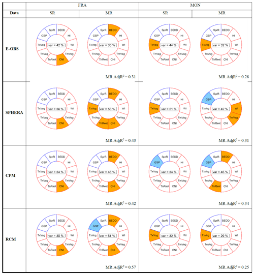
An overview of the performance of the single regression method (SR) and the multiple regression method (MR) is presented in Fig. 10, showing that using a linear combination of bioclimatic indices increases the proportion of explained total productivity variability, especially for FRA.

Figure 10 (a) The maximum fraction of the wine grape productivity variance (%) explained by SR and MR in each consortium; colors indicate the type of climatic data used, and a square (triangular) shape indicates a multiple regression (single regression) approach. (b) Variance differences in percentage between MR and SR for FRA and MON.

Overall, the bioclimatic indices explain a higher proportion of productivity variance in FRA compared to MON (Fig. 10a and Table A8), in line with previous findings at the regional level for LOM and TOS (Massano et al., 2023). The highest proportion of explained variance in productivity is obtained in FRA with the MR approach and RCM data (64 %), followed by SPHERA (56 %) and CPM (48 %). The variance explained in MON is lower, with a maximum of 45 % obtained for CPM and the MR approach, very close to SPHERA with MR (42 %) and to E-OBS with SR (44 %).

The maximum variance in productivity explained by the SR is compared with the MR variance (Fig. 10b). The comparison demonstrates that the MR better represents productivity variability in FRA in all cases except E-OBS, which shows a slight decrease in performance (−7 %). Meanwhile, SPHERA gains 20 %, the CPM 14 %, and the RCM 29 % when MR is compared to SR. In MON, MR provides a better explanation for productivity variance in the SPHERA reanalysis and CPM simulation, accounting for an increase of 11 % and 21 %, respectively. However, for the E-OBS dataset and RCM simulation, MR performance decreases slightly (−12 % and −3 %, respectively). Note that the decrease in performance from the SR to MR method only occurs when only one bioclimatic index is selected in the MR. This could be linked to a coefficient included in the MR (i.e., productivity = a₁ ⋅ index₁) or to the different type of correlation used in SR (Spearman) and MR (Pearson).

4 Discussion and conclusion

This study represents, to the best of the authors' knowledge, the first application of a CPM to investigate the impact of climate variability and change on wine grape productivity through the use of bioclimatic indices. The CPM simulation is compared with an RCM simulation, SPHERA reanalysis, and E-OBS observations for the period 2000–2018. The study presented here focuses on the local scale using wine grape productivity data from two Italian wine consortia, namely Consorzio per la tutela del Franciacorta (FRA) and Consorzio Del Vino Nobile di Montepulciano (MON). A multiple regression approach is used, in addition to a single regression method, to account for the possible interplay of bioclimatic indices in explaining wine grape productivity variability.

Overall, the single regression exhibits high correlation coefficients, but statistically significant results are only found for a small number of indices at the 95 % confidence level. When more than one bioclimatic index is relevant, the multiple regression method outperforms the single regression systematically, enhancing the explanatory power of bioclimatic indices regarding productivity variability. Furthermore, the method has the potential to select the predictors that are fit for purpose.

In FRA, the correlation coefficients are exclusively positive and statistically significant only for temperature-based indices such as BEDD, CNI, and TnRest. Correlations with precipitation-based indices in FRA are not significant and tend to show negative relationships with productivity. These findings suggest that temperature is the main factor affecting production, while precipitation has a negative impact on productivity, potentially resulting in losses due to fungal diseases in the region.

The MON results indicate that only the convection-permitting resolution of the CPM and SPHERA provides statistically significant results for a precipitation-based index (GSP), highlighting the importance of kilometer-scale resolution when precipitation is a dominant factor for productivity. Also, RCM and E-OBS in this region show positive correlations between precipitation-based indices and productivity, even if they are not significant. This differs from the findings for FRA, where the correlations are negative, even if not significant. However, it is worth noting that there are many differences in the geographical features and types of wine produced in FRA and MON. FRA is in the humid subtropical climatic zone, while MON is situated in the hot summer Mediterranean zone. Other factors, such as vintage management techniques and cultivar selection, can also influence the productivity variability in addition to climate, but the investigation of these factors is beyond the scope of this paper. Meanwhile, the productivity for both FRA and MON exhibits a negative correlation with TxVeg with all the climatic data considered, but it is only significant for MON. This suggests that extreme maximum temperatures during the vegetative season (1 April–30 October) may have harmful effects.

These results, which are obtained at the local scale using data from wine consortia, complement and expand the previous study conducted at the regional scale by Massano et al. (2023) using ISTAT productivity data and E-OBS (v26, resolution ∼ 11 km) climate data. In fact, they did not find any statistically significant correlations for the LOM or TOS regions, where FRA and MON are respectively located, with neither temperature-based nor precipitation-based indices. To the contrary, in this work the MR can explain up to 64 % in FRA with the RCM and 45 % in MON with the CPM. This indicates that working at a local scale and including a larger variety of bioclimatic indices is crucial to improve the portion of productivity variance explained by the bioclimatic indices.

The reanalysis dataset SPHERA outperforms the observational dataset E-OBS in both MON and FRA with the MR approach, confirming it to be a valuable alternative to observations. When the MR approach is applied, climate models appear to be a useful tool to explain the variability of productivity, improving the results obtained using E-OBS. However, the use of the CPM does not show a clear added value with respect to the RCM, since it performs better in MON but not in FRA. This could be linked to the fact that temperature is generally the main driver of wine grape production, and the added value of the CPM becomes more evident when precipitation is a dominant factor, as in MON. Nevertheless, in a changing climate, with precipitation frequency and intensity expected to change (Tramblay and Somot, 2018; Zittis et al., 2021), the relevance of precipitation, along with precipitation-based bioclimatic indices, for grape productivity might increase and in turn the use of CPMs might become crucial. The analysis presented here paves the way to the use of climate models to investigate the impact of climate change on wine production in the future. In this context, CPMs can provide new climate information, such as hail risk, which is a convection-related phenomenon that impacts grape productivity. Moreover, this work shows an application of the bioclimatic indices to wine grape productivity that is rarely used.

Appendix A

Table A1 Results of Welch's t test applied to regional and consortia productivity data: t statistics (t), reference value for t (t_ref), and degrees of freedom (DoF) for the t test based on the number of observations computed according to Welch's equation for effective degrees of freedom (Welch, 1938) are displayed. Values of t lower than t_ref indicate that consortium and regional productivity samples come from the same population at a 95 % level of confidence. In the last column is the temporal correlation coefficient (r) computed between consortium and regional productivity data. Asterisks (^*) indicate statistically significant correlations (p≤0.05).

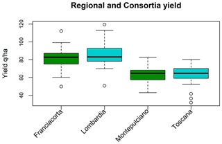
Figure A1 Box plots of regional (cyan) and consortia (green) productivity. The series of LOM and TOS come from the ISTAT database and cover the period 1980–20419, with a 6-year gap between 2000–2005; the period available for FRA is 1997–2019 (calculated by aggregating the Franciacorta DOCG and Curtefranca DOC denominations) and for MON is 1989–2019 (calculated by aggregated the Vino Nobile and Rosso di Montepulciano denominations), with no gap in the series.

Table A2 Spearman correlation coefficient (ρ), the root mean squared error (RMSE) between SPHERA (E-OBS) and CPM, as well as between SPHERA (E-OBS) and RCM time series, and the normalized root mean square error (NRMSE) with respect to the range of values (y_max–y_min) of the reference (SPHERA and E-OBS) in the FRA and MON areas. Asterisks (^*) indicate statistically significant correlations (p≤0.05).

Table A3 Results of Welch's t test applied to mean (TM), maximum (TX), and minimum (TN) temperatures and precipitation (P) from E-OBS, SPHERA, RCM, and CPM datasets for FRA and MON: t statistics (t), reference value for t (t_ref), and the degrees of freedom (DoF) for the t test based on the number of observations computed according to Welch's equation for effective degrees of freedom (Welch, 1938) are displayed. Values of t higher than t_ref indicate that the samples from climate model simulations and the reference datasets come from different populations at a 95 % level of confidence. Asterisks (^*) indicate the means, showing statistically significant differences.

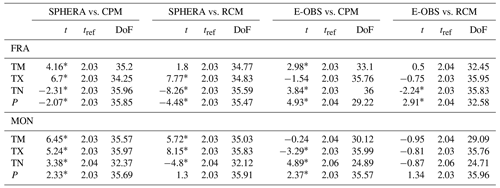
Table A4 Results of Welch's t test applied to the bioclimatic indices from E-OBS, SPHERA, RCM, and CPM datasets for FRA and MON: t statistics (t), reference value for t (t_ref), and the degrees of freedom (DoF) for the t test based on the number of observations computed according to Welch's equation for effective degrees of freedom (Welch, 1938) are displayed. Values of t higher than t_ref indicate that the samples from climate model simulations and the reference datasets come from different populations at a 95 % level of confidence. Asterisks (^*) indicate the means, showing statistically significant differences.

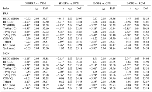
Table A5 Sen's slope estimator, a statistical measure to evaluate the magnitude of the trend, for the FRA area. An asterisk (^*) indicates a significant trend (p≤0.05).

Table A6 Sen's slope estimator, a statistical measure to evaluate the magnitude of the trend, for the MON area. An asterisk (^*) indicates a significant trend (p≤0.05).

Table A7 Sen's slope of the productivity in FRA and MON. Sen's slope is a statistical measure used to calculate the rate of change in a variable over time based on the Sen's estimator. An asterisk (^*) indicates a significant trend (p≤0.05).

Table A8 Ranking of the maximum variance (%) explained for each dataset for each consortium, with an indication of the type of method used (SR: single regression, MR: multiple regression).