A globally applicable framework for compound flood hazard modeling

Coastal river deltas are susceptible to flooding from pluvial, fluvial, and coastal flood drivers. Compound floods, which result from the co-occurrence of two or more of these drivers, typically exacerbate impacts compared to floods from a single driver. While several global flood models have been developed, these do not account for compound flooding. Local-scale compound flood models provide state-of-the-art analyses but are hard to scale to other regions as these typically are based on local datasets. Hence, there is a need for globally applicable compound flood hazard modeling. We develop, validate, and apply a framework for compound flood hazard modeling that accounts for interactions between all drivers. It consists of the high-resolution 2D hydrodynamic Super-Fast INundation of CoastS (SFINCS) model, which is automatically set up from global datasets and coupled with a global hydrodynamic river routing model and a global surge and tide model. To test the framework, we simulate two historical compound flood events, Tropical Cyclone Idai and Tropical Cyclone Eloise in the Sofala province of Mozambique, and compare the simulated flood extents to satellite-derived extents on multiple days for both events. Compared to the global CaMa-Flood model, the globally applicable model generally performs better in terms of the critical success index (−0.01–0.09) and hit rate (0.11–0.22) but worse in terms of the false-alarm ratio (0.04–0.14). Furthermore, the simulated flood depth maps are more realistic due to better floodplain connectivity and provide a more comprehensive picture as direct coastal flooding and pluvial flooding are simulated. Using the new framework, we determine the dominant flood drivers and transition zones between flood drivers. These vary significantly between both events because of differences in the magnitude of and time lag between the flood drivers. We argue that a wide range of plausible events should be investigated to obtain a robust understanding of compound flood interactions, which is important to understand for flood adaptation, preparedness, and response. As the model setup and coupling is automated, reproducible, and globally applicable, the presented framework is a promising step forward towards large-scale compound flood hazard modeling.

1 Introduction

Coastal river deltas are susceptible to flooding due to their physical setting in low-elevation regions and the presence of many densely populated cities. A recent study showed that deltas contained 4.5 % of the global population in 2017 while only covering 0.57 % of the earth's land surface area (Edmonds et al., 2020). Floods in coastal delta regions can occur as the result of different physical drivers, including extreme rainfall, river discharge, or extreme coastal water levels. Floods can also occur because of (or be exacerbated by) the co-occurrence of combinations of these drivers, so-called compound flood events, which may amplify the total flood hazard (Leonard et al., 2014; Zscheischler et al., 2018). Tropical Cyclone Idai, which made landfall near Beira, Mozambique, in March 2019, caused more than 600 casualties and affected an estimated 1.85 million people (UN OCHA, 2019). This is an example of the devastating impacts that compound floods can cause (Emerton et al., 2020). A comprehensive understanding of flood risk in deltas is therefore crucial for effective risk reduction.

There is wide recognition that interactions between flood drivers should be taken into account for flood risk assessment and management in both scientific (Moftakhari et al., 2017; Wahl et al., 2015; Ward et al., 2018) and decision-making communities (Browder et al., 2021; UNDRR, 2019). Several studies have used statistical models to assess the dependence between flood drivers in order to understand the likelihood of extreme drivers occurring together (Camus et al., 2021; Couasnon et al., 2020; Bevacqua et al., 2019; Hendry et al., 2019; Ward et al., 2018). Furthermore, hydrodynamic model simulations have been used to understand the complex physical interactions between drivers and their relative importance for the total flood hazard (Bakhtyar et al., 2020; Eilander et al., 2020; Gori et al., 2020a; Harrison et al., 2021; Kumbier et al., 2018; Muñoz et al., 2021; Olbert et al., 2017; Santiago-Collazo et al., 2019; Torres et al., 2015)

However, to date most global flood risk models still analyze each flood driver in isolation (Alfieri et al., 2017; Hirabayashi et al., 2021; Tiggeloven et al., 2020; Vousdoukas et al., 2018; Ward et al., 2020). Recently, the effect of storm surge on fluvial flooding was analyzed at the global scale, showing that 1-in-10-year fluvial flood levels are exacerbated by surge for 64 % of the locations analyzed, causing increased flood risk for 9.3 % of the population exposed to riverine flooding (Eilander et al., 2020; Ikeuchi et al., 2017). Bates et al. (2021) were the first to make a combined risk assessment of fluvial, pluvial, and coastal flood hazard for the continental USA but did not account for physical interactions of pluvial with other flood drivers.

While the performance and resolution of large-scale flood models are approaching those of local-scale flood models in data-rich areas (Wing et al., 2021), there are still large differences between global flood models in many areas globally (Aerts et al., 2020; Bernhofen et al., 2018; Trigg et al., 2016). The setup of these models remains a challenging task due to the lack of open and accurate high-resolution global topography data (Hawker et al., 2018b) as well as missing data on river and estuarine bathymetry (Neal et al., 2021) and flood defenses (Ward et al., 2015; Wing et al., 2019). Therefore, building hydrodynamic flood models from global datasets requires several data preprocessing steps that may have a large effect on the model skill (Sampson et al., 2015). Furthermore, the code for setting up most global flood models is closed source, while an open-source framework would increase the comparability and reproducibility by providing a transparent workflow (Hall et al., 2022; Hoch and Trigg, 2019). Sosa et al. (2020) presented an automatic model builder for LISFLOOD-FP models, and Uhe et al. (2021) extended this framework to a model cascade to compute fluvial flood hazard from meteorological drivers. Van Ormondt et al. (2020) developed Delft Dashboard, which is a graphical user interface with various modular toolboxes to semi-automatically set up hydrodynamic model schematizations in the ocean and coastal domains but lacks tools to couple riverine models. This leaves a gap for a fully automated model builder that can be applied to the complex coastal delta environment to simulate compound flood events.

In this study we present an automated framework to model compound flooding anywhere on the globe in a reproducible and transparent manner. The framework consists of a 2D hydrodynamic model, which is automatically built from global datasets and coupled with a global hydrological and river routing model for upstream boundary conditions and a global surge and tide model for downstream boundary conditions. The goal of this study is to present the framework, to test its ability to simulate compound floods in data-sparse coastal deltas, and to demonstrate how it can be used for compound flood analysis. In particular, we compare flood hazard maps from the local hydrodynamic model against satellite-derived flood extents for two historical events. To evaluate the added value of using the globally applicable model, we also compare against a global model. Furthermore, we identify the main flood drivers and transition zones between drivers following Bilskie and Hagen (2018).

2 Case study

To evaluate the flood hazard framework, we apply it to two historical events in the Sofala province of Mozambique, namely Tropical Cyclone Idai in March 2019 and Tropical Cyclone Eloise in January 2021. Both events are examples of compound flood events in a coastal delta. The largest city in the Sofala province is Beira, with more than 500 000 inhabitants and a large port connecting the hinterland with the Indian Ocean. While the city itself is mainly threatened by coastal and pluvial flooding, the deltas of the Pungwe and Buzi rivers are also susceptible to fluvial flooding (Emerton et al., 2020; van Berchum et al., 2020).

Tropical Cyclone Idai originated in the Mozambique Channel as a tropical depression, which had already caused extensive flooding after its first landfall in early March. After it moved back over the Mozambique Channel, it gained intensity and became a tropical cyclone with 10 min sustained wind speeds of 165 km h⁻¹, a maximum calculated surge of ∼4.4 m, and torrential rainfall during the second landfall near Beira on 15 March (ERCC, 2019). After the second landfall, large areas flooded, first around the coast and followed a few days later by the Buzi and Pungwe floodplains. The tropical cyclone destroyed more than 60 000 houses, and an estimated 286 000 people received shelter (UN OCHA, 2019).

Tropical Cyclone Eloise made landfall on 23 January 2021 around 20 km south of Beira, with winds of 140 km h⁻¹ and widespread and extreme rainfall. The region experienced widespread post-cyclone flooding, and it had already been hit by heavy rainfall on 15 January and subsequent high river water levels and was still recovering from the 2019 flood after Tropical Cyclone Idai. The Sofala province was the most affected, especially communities along the Pungwe and Buzi rivers. In total, more than 8800 houses were damaged and 176 000 people were affected (UN OCHA, 2021).

These events were selected because they provide a unique case study of two different compound flood events in the same study area, allowing for a comparison of the compound flood dynamics between both events. Furthermore, the lack of compound flooding in global models has been identified as a key limitation to support decision-making in this area (Emerton et al., 2020).

3 Methods

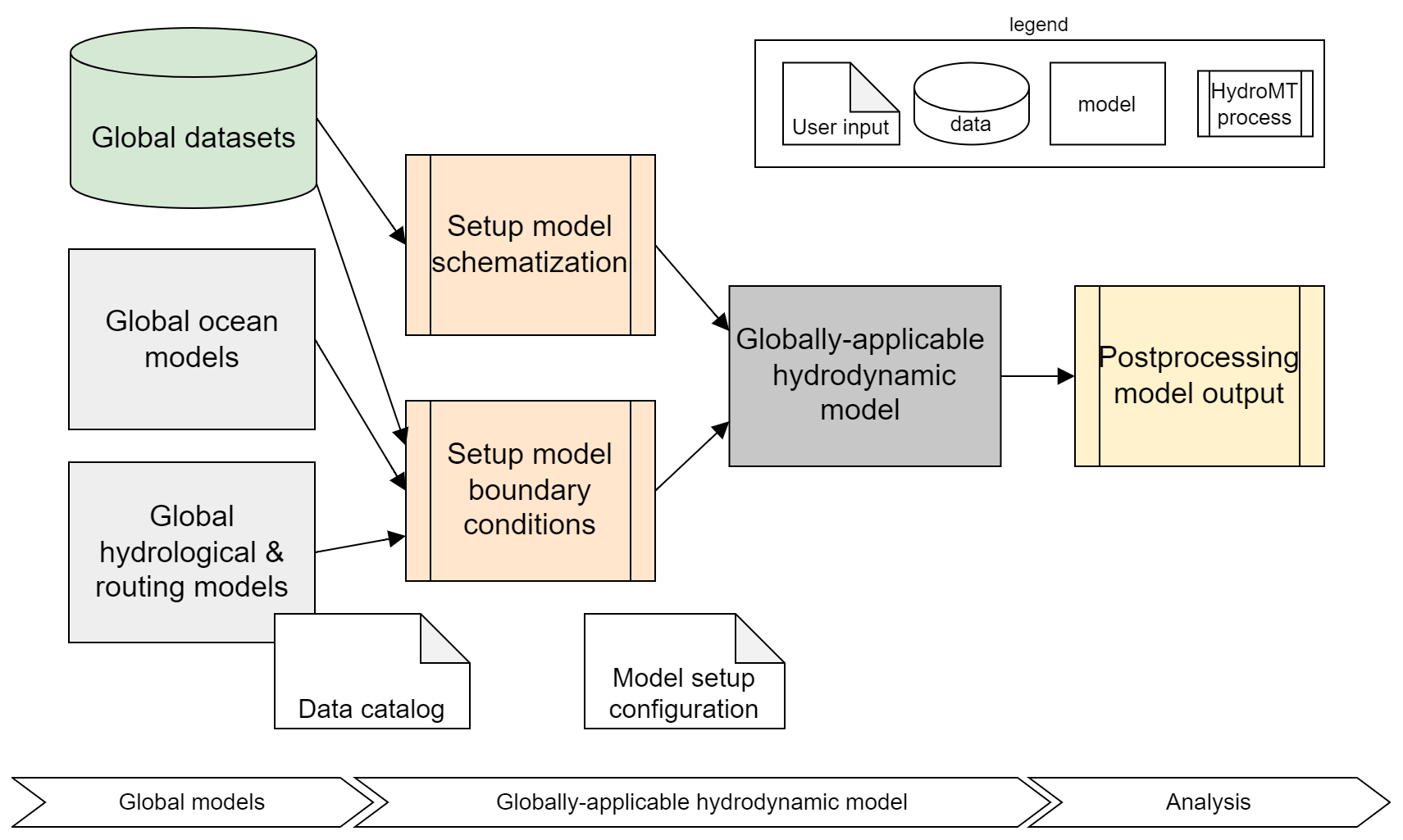
The globally applicable compound flood hazard framework is shown in Fig. 1. In Sect. 3.1 we describe the global models used to set the boundary conditions of the hydrodynamic model. In Sect. 3.2 we discuss the hydrodynamic Super-Fast INundation of CoastS (SFINCS) model as well as its automated setup. In Sect. 3.3 we discuss the analysis of the model results and the compound flood drivers. Both the model setup and analysis (postprocessing) are facilitated by HydroMT v0.4.5 (Eilander and Boisgontier, 2022), an open-source Python package to automate the building and analysis of geoscientific models, and its model-specific SFINCS plugin HydroMT-SFINCS v0.2.1 (Eilander et al., 2022). All required model pre- and postprocessing steps have been automated and can thus easily be repeated for different locations. The approach is modular as datasets can easily be interchanged, also for higher-resolution local datasets if available, and many workflows to process raw data into model input data can be reused for different models.

Figure 1 Framework for globally applicable compound flood hazard modeling.

3.1 Global models

To make the framework globally applicable, we make use of global models to force the local flood model. The following sections describe the global ocean models used for the coastal boundary conditions and global hydrological and routing models used for the fluvial boundary conditions. To ensure coherence between the flood drivers, the atmospheric forcing of all models is based on the ERA5 reanalysis dataset, which has a 0.25^∘ spatial resolution (∼30 km) and a 1 h temporal resolution (Hersbach et al., 2020).

3.1.1 Global ocean models

Total nearshore water levels consist of several components, namely astronomical tide, storm surge, and wave setup. The latter two are episodic fluctuations due to atmospheric drivers. Storm surge is generated by a storm's winds pushing water onshore and the inverted barometer effects of the pressure (Resio and Westerink, 2008). Wave setup is an episodic wave-driven increase in nearshore water levels resulting from wave shoaling and breaking processes (Bowen et al., 1968).

The tide and surge components are simulated with the Global Tide and Surge Model (GTSM) version 3.0 (Muis et al., 2020), which is based on the Delft3D Flexible Mesh hydrodynamic model software (Kernkamp et al., 2011). The model resolution varies from 25 km in the deep ocean to 2.5 km (1.25 km in Europe) near the coast, and results are stored at a 10 min temporal resolution. Details about GTSM schematization and parameterization are discussed in Muis et al. (2020) and Wang et al. (2021). In this study, GTSM is forced with mean sea level pressure and 10 m meridional (v; northward) and zonal (u; eastward) wind components from ERA5 merged with wind and pressure fields from the Holland parametric wind model (Holland, 1980) based on the International Best Track Archive for Climate Stewardship (IBTrACS; Knapp et al., 2010). The data from the Holland model are described with a polar grid with 36 radials and a radius of 750 km following Dullaart et al. (2021), where the data in the outermost 33 % are linearly interpolated with the background ERA5 data to avoid a wind speed and pressure drop towards the outer rim (Deltares, 2022). The simulated tides are based on tide-generating forces at 60 frequencies without assimilation of satellite altimetry (Irazoqui Apecechea et al., 2017). GTSM has been validated for various historical hurricane events (Dullaart et al., 2020) and for derived return levels (Muis et al., 2020), showing good agreement with observations. Hourly time series of significant height of wind waves (Hs) are extracted at GTSM output locations from the 30 arcmin ERA5 dataset and based on the ECMWF Ocean Wave Model (Bidlot, 2012; Hersbach et al., 2020). We estimate the wave setup component based on 0.2 Hs, which is an often-used approximation for (large-scale) studies (Camus et al., 2021; Vousdoukas et al., 2016; US Army Corps of Engineers, 2002). Finally, time series of total water level (Htwl) are derived by combining the GTSM tide and storm surge components (Hst) with the ERA5 wave setup component (Hs): Htwl = Hst + 0.2 Hs at a 10 min temporal resolution.

Due to a lack of observations from coastal water level gauges, a quantitative validation of the simulated water levels is not possible, but some general observations about the simulated data can be made. The maximum simulated water levels in GTSM during both events (5.0 m + m.s.l. during Idai; 3.8 m + m.s.l. during Eloise) occurred close to neap tide and are caused by surge (3.2 m during Idai; 2.6 m during Eloise) and wind setup (1.2 m during Idai; 0.7 m during Eloise). The maximum surge and its timing during Idai (4.0 m) are in line with the operational forecast of 4.4 m based on the HyFlux2 model forced with NOAA Hurricane Weather Research and Forecasting atmospheric data (ERCC, 2019; Probst and Annunziato, 2019). As tide and wave effects are not simulated by this model, total water levels are not available for comparison. In comparison with the tidal constituents of International Hydrographic Organization (IHO) station at the Port of Beira as retrieved using the Delft Dashboard (van Ormondt et al., 2020), the highest astronomical tide is expected to be around 3.8 m, while our simulations result in 4.5 m, indicating an overestimation. This has however little effect on the maximum water levels, which occurred close to neap tide.

3.1.2 Global hydrological and routing models

Riverine discharge is simulated with the global river routing modeling CaMa-Flood version 4.0.1 (Yamazaki et al., 2013; Hirabayashi et al., 2021). CaMa-Flood is selected as to our knowledge it is the only global river routing model with an explicit representation of floodplains (Zhao et al., 2017) that also accounts for downstream sea level boundary conditions (Ikeuchi et al., 2017). CaMa-Flood uses the local inertial approximation (Bates et al., 2010) to solve the mass and momentum equations for river and floodplain flows in one dimension (Yamazaki et al., 2013). A model grid cell represents a unit catchment containing a river segment with a rectangular cross section and a floodplain profile based on subgrid topography. In CaMa-Flood version v4.0 and later, the subgrid parameters are based on the global high-resolution topography data MERIT DEM (Yamazaki et al., 2017) and hydrography data MERIT Hydro (Yamazaki et al., 2019). Each river segment is connected to one downstream neighbor, but floodplains of neighboring unit catchments can exchange flows through so-called bifurcation channels, making it a quasi-2D model. The bifurcation channels are based on a set number of elevation thresholds for which a representative stream width at the interface between the floodplains of two neighboring unit catchments is derived based on the subgrid topography. Bifurcation channels are activated if the surface water elevation exceeds an elevation threshold. These bifurcation channels are shown to be important in flat coastal areas to correctly simulate floodplain connectivity (Ikeuchi et al., 2015; Mateo et al., 2017; Yamazaki et al., 2014). The unit-catchment areas are used to interpolate the input runoff to the model grid, where the runoff within the unit catchment directly enters the river segment at its upstream end.

We use a regional cutout between 32 ^∘W, −21.5 ^∘S, 35.5 ^∘E, and −17 ^∘N of the 3 arcmin spatial-resolution global CaMa-Flood schematization; see Fig. 2a. Default model settings are used except for the bifurcation scheme, which is defined at 10 instead of 5 elevation thresholds to maximize floodplain connectivity. Furthermore, to make the model comparable with the globally applicable model, river width and depth maps are created using the same procedure as explained in Sect. 3.2.1 but with the CaMa-Flood river segments. CaMa-Flood is forced with ERA5 runoff, which is simulated with the Hydrological Tiled ECMWF Scheme for Surface Exchanges over Land (HTESSEL) (Balsamo et al., 2009), and total seawater levels from the nearest GTSM output location at all river outlet locations; see Sect. 3.1.1. Grids of instantaneous discharge and flood depth with a daily temporal resolution are saved to be used as input for the local flood model. The flood depth maps at the model resolution are downscaled to a 3 arcsec (∼100 m at the Equator) resolution based on high-resolution topography.

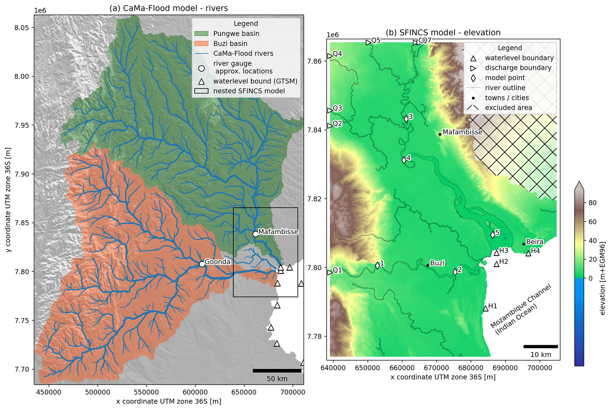
Figure 2 Maps of a regional cutout of the global CaMa-Flood model (a) and the local SFINCS model with boundary conditions and model output point locations for the case study in Sofala province, Mozambique (b). Note that both maps are in different projections based on the projection used for the model schematization.

During Idai, national hydrological bulletins reported water levels for the Pungwe River at Mafambisse and for the Buzi River at Goonda (approximate locations are shown in Fig. 2a). The bulletins report water levels during the onset and recession of the flood peak but miss the peak itself. Furthermore, neither exact locations nor the used vertical reference level could be retrieved, making a quantitative comparison impossible. We therefore only make a qualitative comparison between the observed and CaMa-Flood-simulated water levels. Compared to the observations, the simulated flood peak at the Pungwe River is slightly delayed but seems to correctly capture the recession, while the flood peak at the Buzi River seems to be overestimated and the recession too fast (Fig. A1). The overestimation could be the result of missing schematization of reservoirs in the model, such as the Chicamba reservoir in the Revué River, a tributary to the Buzi River.

3.2 Hydrodynamic model

The SFINCS model (Leijnse et al., 2021) is used to simulate water levels and overland flood depths within coastal deltas. SFINCS is selected as it is designed to efficiently simulate overland flow from compound flooding at limited computation costs and with good accuracy (Leijnse et al., 2021; Sebastian et al., 2021). The governing equations of the SFINCS model are based on the local inertial equations in two dimensions (Bates et al., 2010). First, the flow rate is solved based on two 1D momentum equations in x and y directions with spatially varying roughness. Then, the water levels are computed based on the mass balance. On-grid precipitation and discharge boundary conditions are added as a local source term in the mass equation. At open boundaries, the model is forced with dynamic water levels, which are interpolated from the two nearest user-defined point locations with water levels. For a full description of the model, we refer the reader to Leijnse et al. (2021). Here we use the SFINCS code revision 295.

In the remainder of this section we describe the steps taken to automatically set up the SFINCS model schematization and forcing from global datasets using HydroMT-SFINCS v0.2.1 (Eilander et al., 2022). The complete model setup process is described in a single configuration .ini file, and all datasets (see Table 1) are described in a single data catalog .yaml file; see Appendix B. This improves the transparency and reproducibility of the model setup.

Table 1 Overview of global datasets used to set up the hydrodynamic flood model.

3.2.1 Setup of model schematization

Step 1: model grid definition

The SFINCS model grid is set up based on a bounding box of the area of interest; a resolution; and a projected coordinate reference system, here between 34.33^∘ W, −20.12^∘ S, 34.95^∘ E, and −19.30^∘ N (WGS84) at 100 m resolution in the UTM zone 36S projection. Cells that are not connected to the Buzi or Pungwe floodplains and drain into adjacent basins are excluded from the model domain.

Step 2: topography and hydrography data

Topography data are reprojected onto the model grid using bilinear interpolation. As hydrography data (D8 flow directions and upstream area) cannot be reprojected directly, we instead reproject a pseudo-topography grid based on the upstream area and subsequently derive flow directions. The upstream area is then recalculated based on the new flow directions, taking into account the upstream area of inflowing rivers and streams at the model domain boundary. The hydrography maps are not used by SFINCS but used at later stages of the automatic model setup to define river bathymetry and river in- and outflow locations. Here we used topography and hydrography data from MERIT Hydro v1.0 (Yamazaki et al., 2019).

Step 3: river and estuarine bathymetry

As global digital elevation models (DEMs) do not represent the bed level of river channels, the river bathymetry is burned into the data using a similar procedure to in Sampson et al. (2015). Rivers are defined based on an upstream area threshold and discretized into river segments. For each segment, we determine first the river width from a binary river mask, then the river bankfull elevation from the cells adjacent to the river mask, and finally the river depth relative to the bankfull elevation. The detailed procedure is explained here.

Rivers are based on D8 flow directions and a minimal upstream area threshold. River segments are defined between river confluences or a river headwater cell or outlet cell and a confluence. Long segments are split into equal parts to approximate a user-defined length. Here, we used a minimal upstream area threshold of 100 km² and an approximate segment length of 5 km.

The river width is calculated as the segment average width derived from a binary river mask, by dividing the surface area of each segment by its length, where the areas across multiple parallel estuarine channels are summed. The mask is primarily based on the Global River Widths from Landsat (GRWL) Database (Allen and Pavelsky, 2018) but is extended by rasterizing the river width from the Lin et al. (2020) dataset. This dataset contains river width estimates for ∼1.6 km river segments based on a machine learning approach that uses 16 covariates and was trained based on an average width from GRWL and MERIT Hydro. Compared to MERIT Hydro or GRWL, it has a higher spatial coverage and extends to smaller rivers with a minimum width of 30 m.

The river bankfull elevation, relative to the segment elevation, is estimated from a low percentile of height above the nearest river values of cells neighboring the river mask. These values are then corrected such that the absolute bankfull elevation levels are monotonically increasing in an upstream direction using the algorithm developed by Yamazaki et al. (2012). Here we use the 25th percentile, which was found to give good results for this region but might need to be refined for other regions.

We distinguish between a fluvial and estuarine part of the river to determine the river depth. The riverine depth h (m) is estimated from the bankfull discharge Q (m³ s⁻¹) using a power-law relationship: h=aQ^b, where the default values for a (0.27) and b (0.30) are based on Andreadis et al. (2013). The bankfull discharge is based on the 1-in-2-year return values of the discharge as simulated by Lin et al. (2019), and it is derived from the nearest river segment from the Lin et al. (2020) dataset. Gaps in bankfull discharge data are filled based on the nearest valid upstream value. The estuarine depth is kept constant based on the depth of the most upstream estuarine segment, which provides a first-order approximation of the depth in ungauged estuaries and is in accordance with observed depths in ideal alluvial estuaries in low-gradient regions (Gisen and Savenije, 2015). Estuarine segments are classified based on a width convergence rate. Natural alluvial estuaries have a funnel planform shape that is wide at the ocean and narrows inland (Savenije, 2015). Here we use a convergence rate threshold of 0.01 m m⁻¹ applied to a smoothed segment average width. This value was found based on trial and error for the estuaries under consideration and might need to be refined for other locations. A global minimum river depth of 0.5 m is used.

The riverbed elevation zb [m + EGM96] is calculated for each model cell of a river segment from the cell elevation z0 [m + EGM96], relative bankfull elevation difference dz (m), and the bankfull depth h (m): $zb=z\mathrm{0}+\max (\mathrm{0},\mathrm{d}z-h)$. This bed level is burned into the river center cells and spread to neighboring cells within the river mask to burn a rectangular river profile in the DEM.

Finally, we ensure that each river cell has at least one horizontally or vertically neighboring cell with the same or lower elevation to ensure the river has D4 connectivity in the model.

Step 4: Manning roughness

A spatially varying Manning roughness grid is set up that differentiates between land and river cells, based on the river mask as defined in the previous step. Here we used a constant of 0.03 s m${}^{-\mathrm{1}/\mathrm{3}}$ for river cells and 0.1 s m${}^{-\mathrm{1}/\mathrm{3}}$ for land cells, which is in line with other studies (e.g., Di Baldassarre et al., 2009) and consistent with the global CaMa-Flood model (Yamazaki et al., 2011). HydroMT-SFINCS also contains a routine to set up a spatially varying roughness grid based on land-cover data, which is not used here to keep the model consistent with CaMa-Flood.

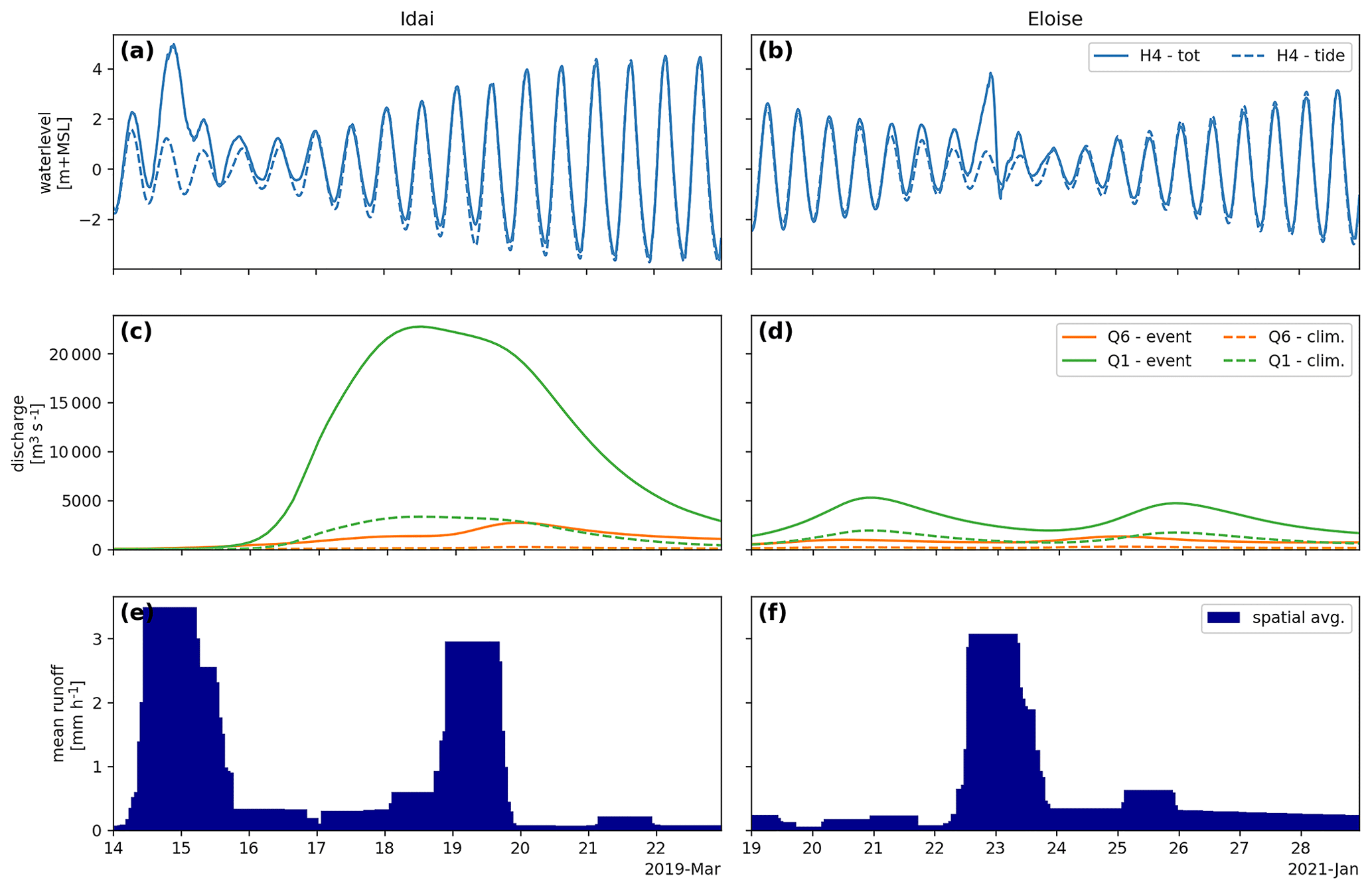
Figure 3 SFINCS boundary conditions during Tropical Cyclone Idai (a, c, e) and Tropical Cyclone Eloise (b, d, f) for the total sea level from GTSM and ERA5 (a, b), discharge from CaMa-Flood (c, d), and spatial average runoff from ERA5 (e, f). The solid lines show the total water levels and discharge, as used for the validation; see Sect. 3.3.1. The dashed lines show the tidal water level component only (a, b) and normalized discharge to match the climatological mean (c, d), as used in the compound driver analysis; see Sect. 3.3.3. Only one coastal location (H4) and the two main rivers (Q1 – Buzi and Q6 – Pungwe) are shown to improve the readability of the plots. The labels in the legends correspond to the boundary locations as shown in Fig. 2b.

Step 5: boundary cells

By default, the cells at the edge of the model domain have closed boundaries, but these can be changed to Riemann-type open water level boundaries. Here, an open water level boundary is set for all cells at the interface with the ocean by intersecting the model domain edge cells with the OSM ocean shapefile (FOSSGIS, 2020). In the absence of water level forcing of rivers leaving the model domain at the south and east model boundaries and to avoid water building up within the model domain, open boundary cells with a zero water depth are set at these locations. These open boundary cells are derived from the previously set hydrography data based on a user-defined upstream area threshold and a river width, here 10 km² and 1 km respectively.

Step 6: river inflow points

Discharge boundary conditions are set at source point locations within the model domain. These points are based on cells where a river flows into the model domain. Rivers are based on a user-defined upstream area and river length thresholds and derived from the hydrography data as derived previously. The minimum length threshold is used to filter short river segments that flow in and out of the model domain. Here we use an upstream area threshold of 100 km² and minimum length of 10 km to force the model with discharge from seven rivers flowing into the model domain; see Fig. 2b.

3.2.2 Setup of model boundary conditions

SFINCS is forced based on output from global models, which is automatically transformed into the input data format that SFINCS requires. This is also referred to as a loose coupling between models (Santiago-Collazo et al., 2019). The following steps, dealing with dynamic boundary conditions, are repeated for each event and/or sensitivity scenario (see Sect. 3.3.3). The model boundary conditions for both historical events are shown in Fig. 3.

Step 7: coastal boundary

Water level boundary conditions are defined at point locations and interpolated by SFINCS to the nearest water level boundary cell. Water level data for the model simulation time period are selected from (global) water level point time series datasets based on a maximum distance from the water level boundary cells (step 5 in Sect. 3.2.1). The water level data can optionally be corrected for the offset between the vertical datum of the water level and topography data. Here, we use a maximum distance of 5 km to select GTSM output locations and correct these for the difference between m.s.l. and the EGM96 vertical datum based on the CNES-CLS18 mean dynamic topography (Mulet et al., 2021). Note that this offset amounts to ∼0.8 m on average for the selected output locations. The total water level time series at a representative location for both events are shown in the top panels of Fig. 3 (solid line).

Step 8: fluvial boundary

Discharge boundary conditions are defined at source point locations (step 6 in Sect. 3.2.1) within the model domain. Discharge data for the simulation time period are selected from a gridded discharge dataset. As the (global) discharge dataset is typically based on another (coarser-resolution) river network, the source point locations must be matched with a corresponding river cell, which is not necessarily at the exact same location. A matching river cell is defined as the cell within a user-defined maximum search radius that has the smallest difference in the upstream area with the inflow point location, which is at least smaller than a user-defined threshold for the absolute or relative difference. Here, we select discharge from the gridded CaMa-Flood model output within a one-cell search window around the source point location based on a maximum relative error of 5 % and maximum absolute error of 100 km² in the upstream area. The discharge time series at the two main rivers for both events are shown in the center panels of Fig. 3 (solid line).

Step 9: pluvial boundary

We use spatially varying precipitation fields for direct rainfall-on-grid forcing. The data are derived from (global) gridded precipitation datasets for the model domain and simulation time period and reprojected onto the model projected coordinate system in a resolution similar to the source resolution. Here we use ERA5 runoff rather than precipitation to account for hydrological processes such as infiltration and evaporation and to ensure comparability with the global CaMa-Flood model. Note that infiltration can also be simulated within SFINCS but was turned off for this experiment as this process is accounted for by using runoff instead of precipitation data. The spatially average runoff time series for both events are shown in the bottom panels of Fig. 3.

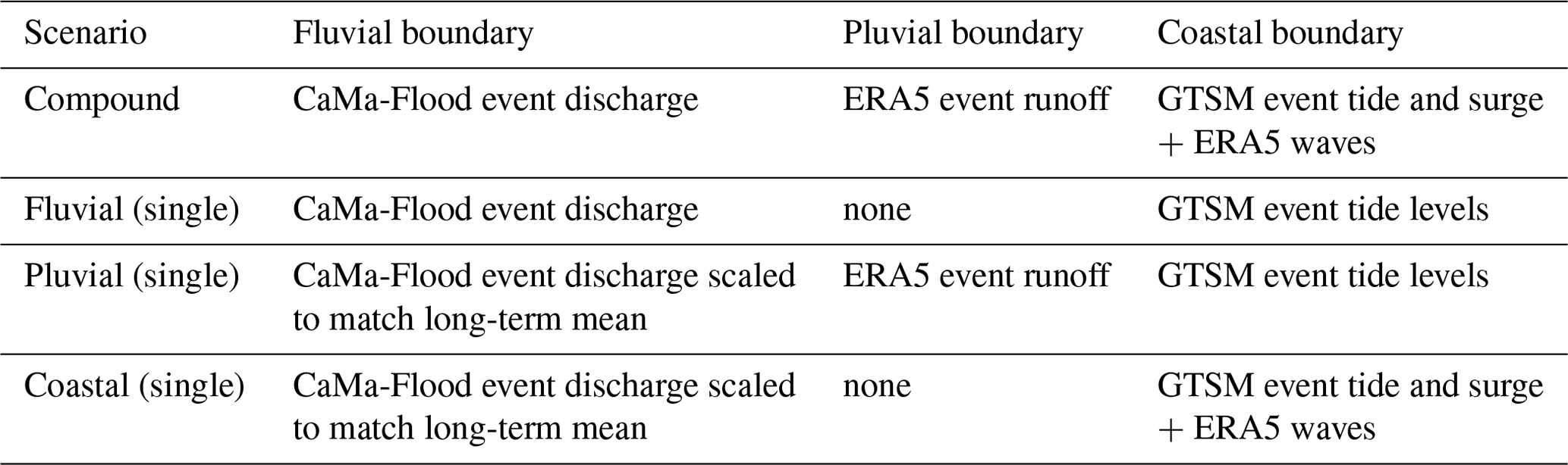
Table 2 Overview of model sensitivity runs. N/A stands for not applicable.

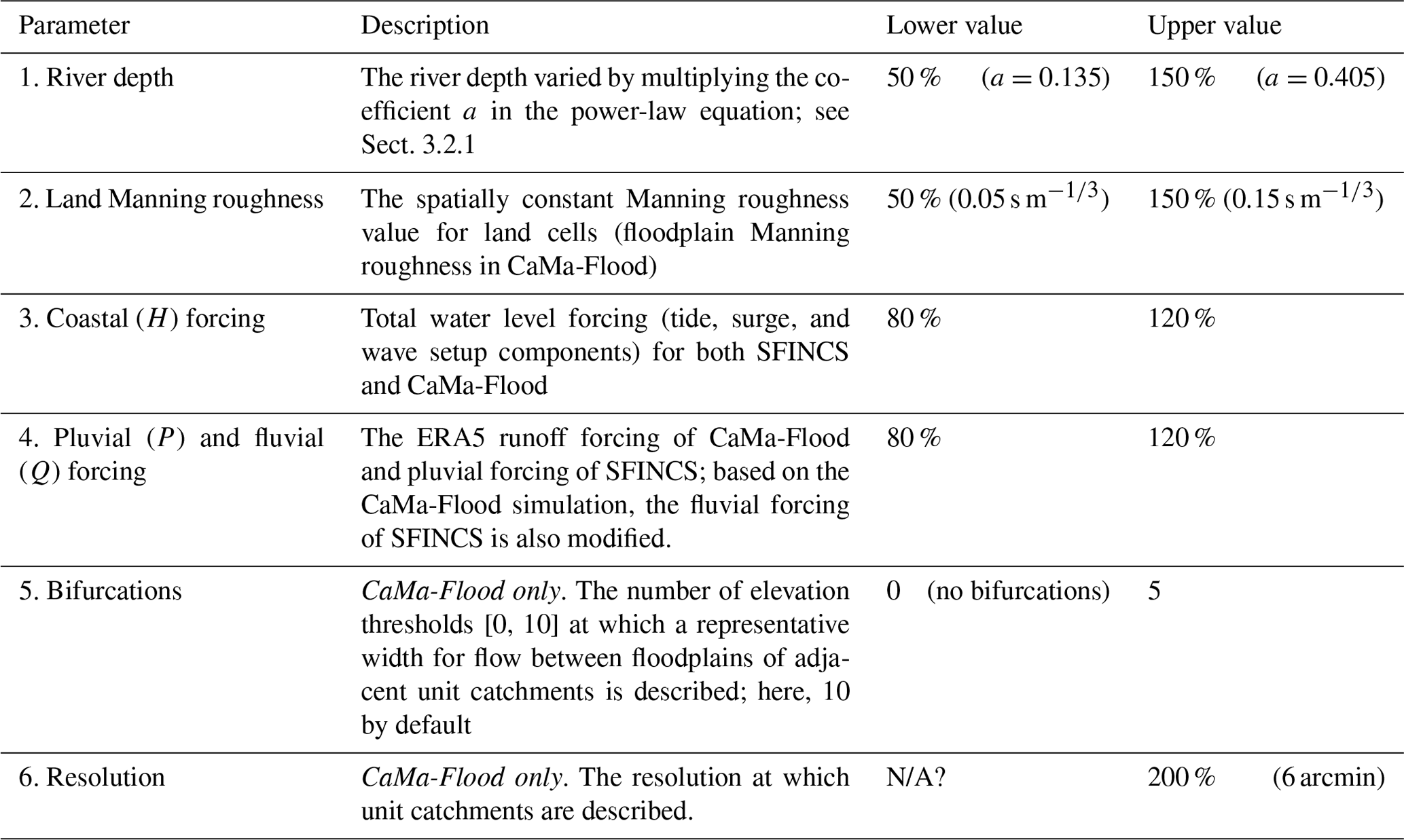
Table 3 Overview of model boundary conditions in compound- and single-driver scenarios.

3.3 Analysis of the model results

3.3.1 Validation against observed flood extent

As no quantitative streamflow or water level observation data are openly available for this location, we focus on a comparison between satellite-derived and simulated flood extent. Model skill is quantified based on three metrics that are commonly used to analyze flood models (Vousdoukas et al., 2016; Wing et al., 2021). The model skill is measured by the critical success index (C), which is the ratio of the area that is correctly simulated to be flooded (Fsim∩Fobs) over the union of observed and simulated flooded areas (Fsim∪Fobs), thereby accounting for both over- and underprediction; see Eq. (1). The critical success index ranges from 0 (no match) to 1 (perfect match). The hit rate (H) is the ratio area that is correctly simulated to be flooded over the observed flood extent (Fobs); see Eq. (2). The hit rate ranges from 0 (none of the observed flood extent is flooded in the model) to 1 (the complete observed flood extent is flooded in the model). The false-alarm rate (F) is the ratio of the area which is wrongly simulated to be flooded (Fsim $/$ Fobs) over the observed flood extent; see Eq. (3). The false-alarm rate ranges from 0 (no overprediction) to infinity (1 indicates equally sized areas of wrongly simulated and observed flooding).

$$\begin{array}{}\text{(1)}& C={\displaystyle \frac{\mathrm{Fsim}\cap \mathrm{Fobs}}{\mathrm{Fsim}\cup \mathrm{Fobs}}}\end{array}$$

$$\begin{array}{}\text{(2)}& H={\displaystyle \frac{\mathrm{Fsim}\cap \mathrm{Fobs}}{\mathrm{Fobs}}}\end{array}$$

$$\begin{array}{}\text{(3)}& F={\displaystyle \frac{\mathrm{Fsim}/\mathrm{Fobs}}{\mathrm{Fobs}}}\end{array}$$

High-resolution (10 m) flood extent data are derived from Sentinel-1 synthetic aperture radar (SAR) images. We use VV-polarized ground-range-detected data, provided by Google Earth Engine (GEE), which has undergone geometric terrain correction and provides radar backscatter in decibel (dB) units. These data are processed using the GEE with an unsupervised histogram-based surface water mapping algorithm that consists of three steps (Markert et al., 2020). First, noise is reduced using the refined Lee speckle filter (Lee, 1981). Second, a threshold to distinguish water and dry cells is detected using the edge Otsu thresholding algorithm (Donchyts et al., 2016). Third, cells with a relative elevation of more than 50 m above the nearest stream are excluded from the water class to avoid false positives. We process each image individually and combine flood extents from ascending and descending orbits during the same day. In total we obtain flood extents for four dates based on eight images: on 19 and 20 March 2019 for Tropical Cyclone Idai, which is around the peak of the flood event, and on 25 and 26 January 2021 for Tropical Cyclone Eloise, which is just before the peak of the flood event. Finally, the flood extents are reprojected to the SFINCS model grid.

The simulated flood extent is derived from the maximum flood depth based on cells with a flood depth larger than a 15 cm threshold (e.g., Wing et al., 2017). The same postprocessing is applied to the CaMa-Flood flood depth maps but after downscaling to a 3 arcsec grid (see Sect. 3.1.2) and reprojection to the SFINCS grid using nearest-neighbor interpolation. Cells with permanent water are excluded from the comparison. We compare the individual satellite-derived flood extents with the maximum simulated extent from the same day and the maximum satellite-derived extent per event with the maximum simulated extent during all days with satellite observations.

3.3.2 Sensitivity analysis

We perform a sensitivity analysis of the model skill by varying several model parameters and model forcing for both historical events. A description of each model sensitivity run is provided in Table 2.

3.3.3 Compound flood drivers

To examine the role of each driver and interactions between fluvial, pluvial, and coastal flood drivers on flood levels, we perform a scenario analysis with the SFINCS model where we vary the boundary conditions; see Table 3 for details. During single-driver events, the forcing of both other drivers is adjusted to non-extreme conditions; see dashed lines in Fig. 3. For the fluvial boundary condition, we normalize the event discharge to match the long-term mean discharge; for the pluvial boundary, we set the rainfall to zero; and for the coastal boundary, we use the tidal signal of the event only. We identify transition zones as areas where water levels in the compound scenario are at least 5 cm higher than in any of the single-driver scenarios, in line with earlier studies on compound flooding where thresholds vary between 0–20 (Bilskie and Hagen, 2018; Gori et al., 2020b; Shen et al., 2019). In addition, we identify the main flood driver based on the single-driver scenario that results in the largest water level.

4 Results and discussion

4.1 Model comparison

In this section we present a comparison of the skill of the global CaMa-Flood and local SFINCS models to simulate the flood extent of the historical flood events Idai and Eloise. Both models are forced with the same data, and we used the same Manning roughness and river depth estimation for compatibility. In general, we simulate more widespread flooding during Idai compared to Eloise and with SFINCS compared to CaMa-Flood (Fig. 4). The difference between both models in the Buzi floodplains is likely due to the limited connectivity between floodplains of neighboring cells in the CaMa-Flood model through its so-called bifurcation scheme. This scheme is too limited to represent the connectivity in the large low-gradient floodplains of the Buzi and Pungwe rivers. This can be seen in the downscaled CaMa-Flood flood maps, which show unrealistic sudden local drops in flood depth at the interface of unit catchments (Fig. 4a) and larger simulated water levels in the Buzi in CaMa-Flood compared to SFINCS (Fig. 5a, b). The difference around the Pungwe estuary is likely due to the response of both models to coastal boundary conditions. The response in the Pungwe estuary in CaMa-Flood is more attenuated and slower compared to SFINCS (Fig. 5c, d) due to the lower resolution of the CaMa-Flood model. In addition, some small coastal areas at the estuary mouth which are flooded in SFINCS are not covered by the CaMa-Flood model. The differences around Beira, where no flooding is simulated by CaMa-Flood, can be attributed to the fact that CaMa-Flood does not simulate direct coastal flooding but only the effect of coastal forcing on riverine water levels and subsequent fluvial flooding. Finally, the difference on the hillslopes can be attributed to the fact that CaMa-Flood does not simulate direct pluvial flooding. While in SFINCS the runoff forcing (i.e., net precipitation) is added as a source term to each grid cell, in CaMa-Flood it is directly added to the river component of each unit catchment. Furthermore, the drainage capacity in this area in SFINCS is likely underestimated due to the absence of small (subgrid-scale) streams in the model topography, which is limited by the model resolution.

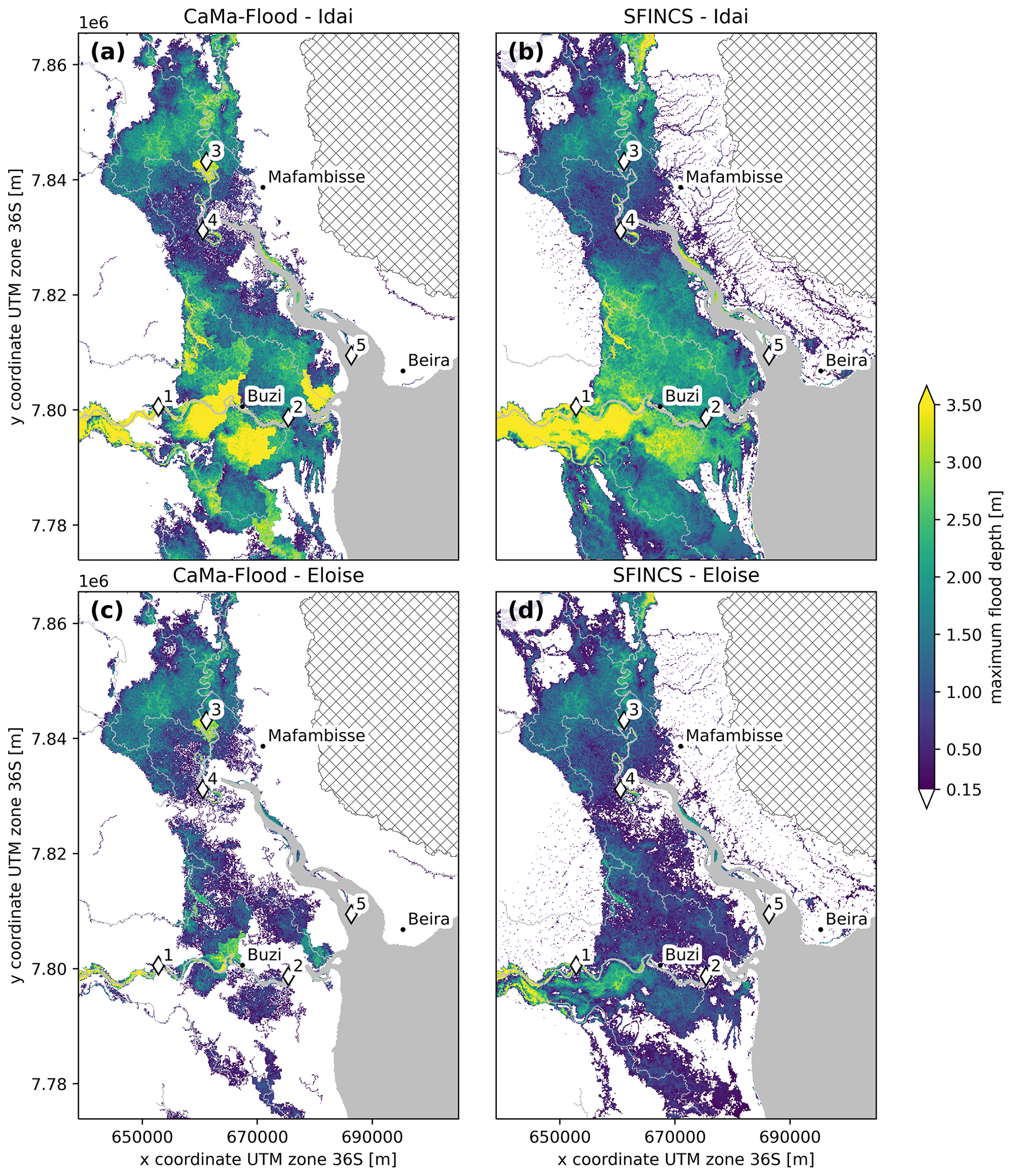
Figure 4 Simulated maximum flood depths from CaMa-Flood (a, c) and SFINCS (b, d) for Tropical Cyclone Idai (a, b) and Tropical Cyclone Eloise (c, d). The diamonds indicate model output point locations for which water level time series are extracted; see Fig. 5. The grey areas indicate permanent water, and the hatched areas are excluded.

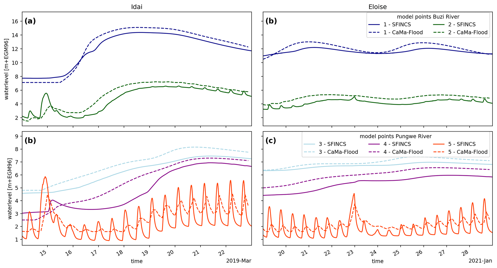
Figure 5 Simulated time series of water levels during Tropical Cyclone Idai (a, c) and Tropical Cyclone Eloise (b, d) with SFINCS (solid lines) and CaMa-Flood (dashed lines) for two locations in the Buzi (a, b) and three in the Pungwe (c, d). See diamonds in Fig. 4 for the exact model output point locations.

Here, we compare simulated flood extents with satellite-derived flood extents for both events. Figure 6 shows the skill calculated from comparing the maximum multi-day flood extents with Sentinel-1 observations. In addition, Table 4 and Figs. A2 and A3 show comparisons of individual satellite-derived extents with the maximum simulated extent during the same day. In general, the skill of both models is higher for the Idai compared to the Eloise flood event. This could be related to the fact that the satellite-derived flood extents for Eloise do not capture the maximum simulated extent. SFINCS shows similar performance to CaMa-Flood in terms of the critical success index for the multi-day maximum extent (C = 0.75 vs. 0.73 during Idai and 0.46 vs. 0.47 during Eloise) but better performance for most individual days (C = 0.75–0.77 vs. 0.68–72 during Idai and 0.47–0.47 vs. 0.45–0.47 during Eloise). There are substantial differences in the simulated flood extents between both models. The SFINCS simulations show larger flood extents compared to CaMa-Flood, resulting in a higher hit ratio (H = 0.94 vs. 0.83 during Idai and 0.82 vs. 0.63 during Eloise) and a higher false-alarm ratio (F = 0.22 vs. 0.14 during Idai and 0.48 vs. 0.35 during Eloise) for the multi-day maximum extents. For individual daily extents, we find the same pattern but with larger differences for the hit rate. The underestimation of CaMa-Flood is concentrated in the floodplains of the Buzi River and around and north of the city of Beira; see orange colors in Fig. 6a and b. The overestimation in SFINCS is concentrated along the banks of the Pungwe River and the hillslopes northeast of it. For Eloise, the flood extent is also overestimated in the floodplains south of the Buzi River; see red colors in Fig. 6c and d.

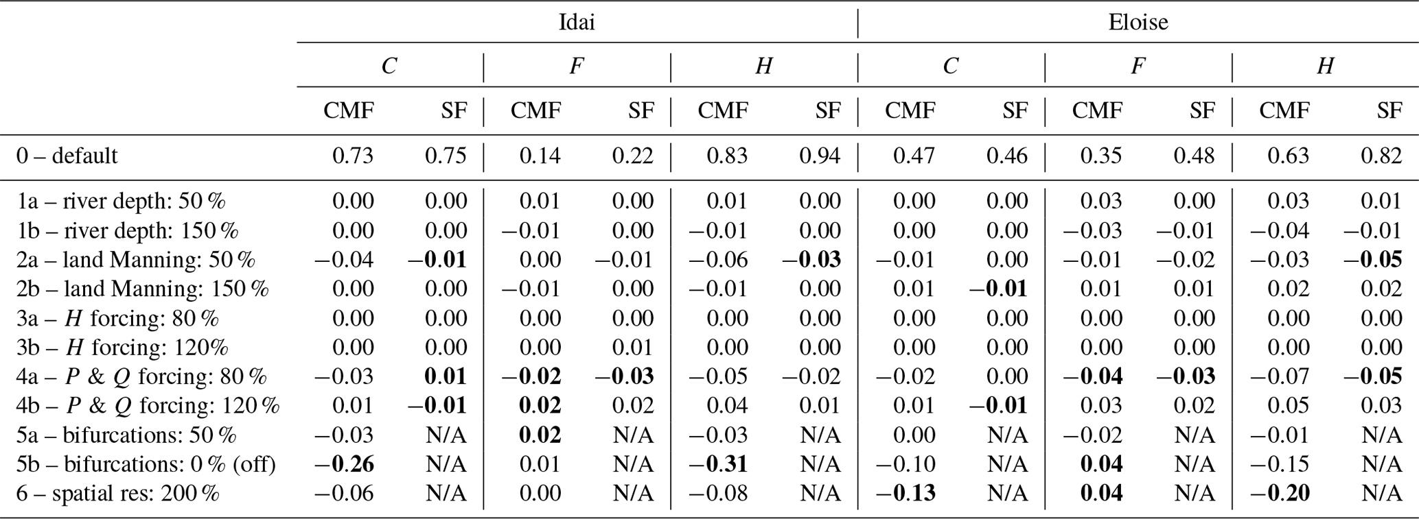
To further investigate the model performance, we performed a sensitivity analysis on some of the most important model parameters and model forcing based on the multi-day maximum flood extents. In general, we find that the skill of both models is not very sensitive to the river depth (Table 5, scenario 1) and the Manning roughness for land cells (Table 5, scenario 2). This is due to the extremeness of the fluvial driver, especially for Idai, during which the river conveyance capacity was small compared to the total discharge. Both models are also not sensitive to changes in the coastal forcing (Table 5, scenario 3) but are sensitive to changes in the pluvial and fluvial forcing (Table 5, scenario 4). This is due to the relatively large fluvial flood driver compared to the coastal flood driver during these two events and the small fraction of the total flood area that is caused by direct coastal flooding (Sect. 4.2). The skill is likely more sensitive to the coastal water level forcing if assessed for a snapshot around the surge peaks of both events instead of the multi-day maximum flood extent, but that is not available. For CaMa-Flood, we find that the model is very sensitive to the presence of bifurcation channels (Table 5, scenario 5) and resolution of the model (Table 5, scenario 6). With fewer bifurcation layers and a coarser model resolution, the connectivity between floodplains reduces, resulting in a large decrease in model skill. Flow connectivity in the model has been shown to be important to correctly simulate inundation dynamics in (coastal) floodplains (Bernhofen et al., 2018; Neal et al., 2012; Trigg et al., 2012). Multiple downstream connectivity, as implemented in the bifurcation scheme of CaMa-Flood, is crucial to adequately simulate floods in deltas (Ikeuchi et al., 2015; Mateo et al., 2017), which is underlined by the results in our study. However, we still find that the flow connectivity is underrepresented compared to the SFINCS mode as shown by the more widespread (fluvial) flooding with SFINCS.

The skill of both models is in line with other flood studies using global models. Global flood models showed C = 0.45–0.70 in comparison with MODIS imagery of three flood events over the African continent (Bernhofen et al., 2018) and C = 0.43–0.65 in comparison with various reference flood maps in Germany and the UK (Alfieri et al., 2014). A LISFLOOD-FP model built with LFPtools was found to have C = 0.63 for a flood event in the River Severn (Sosa et al., 2020). For local fluvial inundation models that are calibrated against flood extent imagery, typical values of C = 0.7–0.9 can be reached, depending on the quality of the flood extent imagery (Di Baldassarre et al., 2009; Horritt and Bates, 2002; Stephens and Bates, 2015; Wood et al., 2016). Our results also demonstrate that a commonly used metric to evaluate flood models such as the critical success index can mask large differences between model results and should be evaluated together with the false-alarm and hit ratios and inspection of the geographical patterns and differences. An additional comparison with flood levels, if available, would allow for a more comprehensive validation (Stephens and Bates, 2015; Wing et al., 2021).

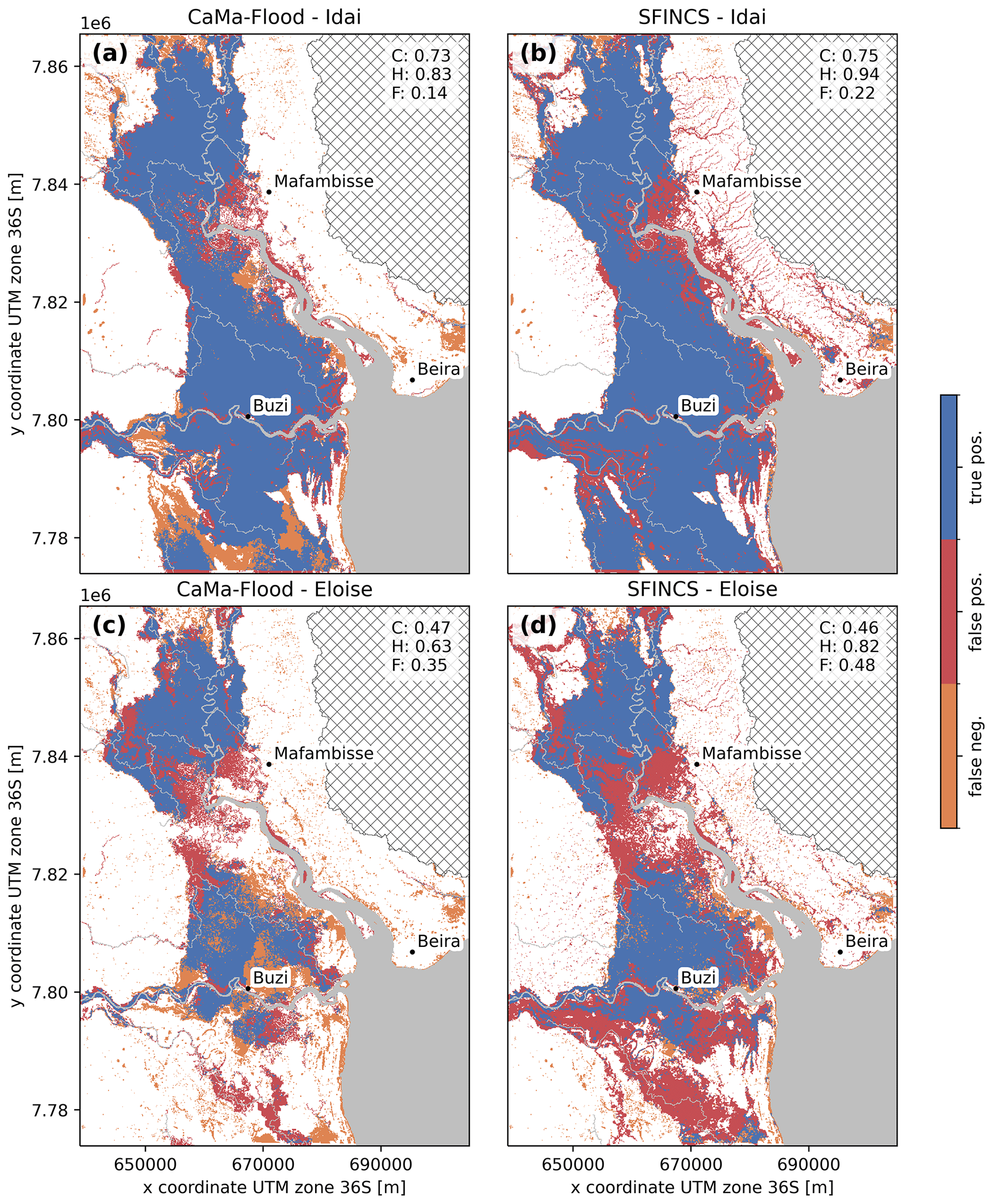
Figure 6 Skill of simulated maximum flood extents from CaMa-Flood (a, c) and SFINCS (b, d) based on satellite-derived flood extents for Tropical Cyclone Idai (a, b) and Tropical Cyclone Eloise (c, d), evaluated based on the critical success index (C), hit rate (H) and false-alarm ratio (F) as shown in the top right of each panel. The grey areas indicate permanent water, and the hatched areas are excluded as these areas drain to other basins.

Table 4 Skill of simulated flood extents from CaMa-Flood (CMF) and SFINCS based on satellite-derived flood extents from individual dates and the maximum flood extent per event, evaluated based on the critical success index (C), hit rate (H) and false-alarm ratio (F).

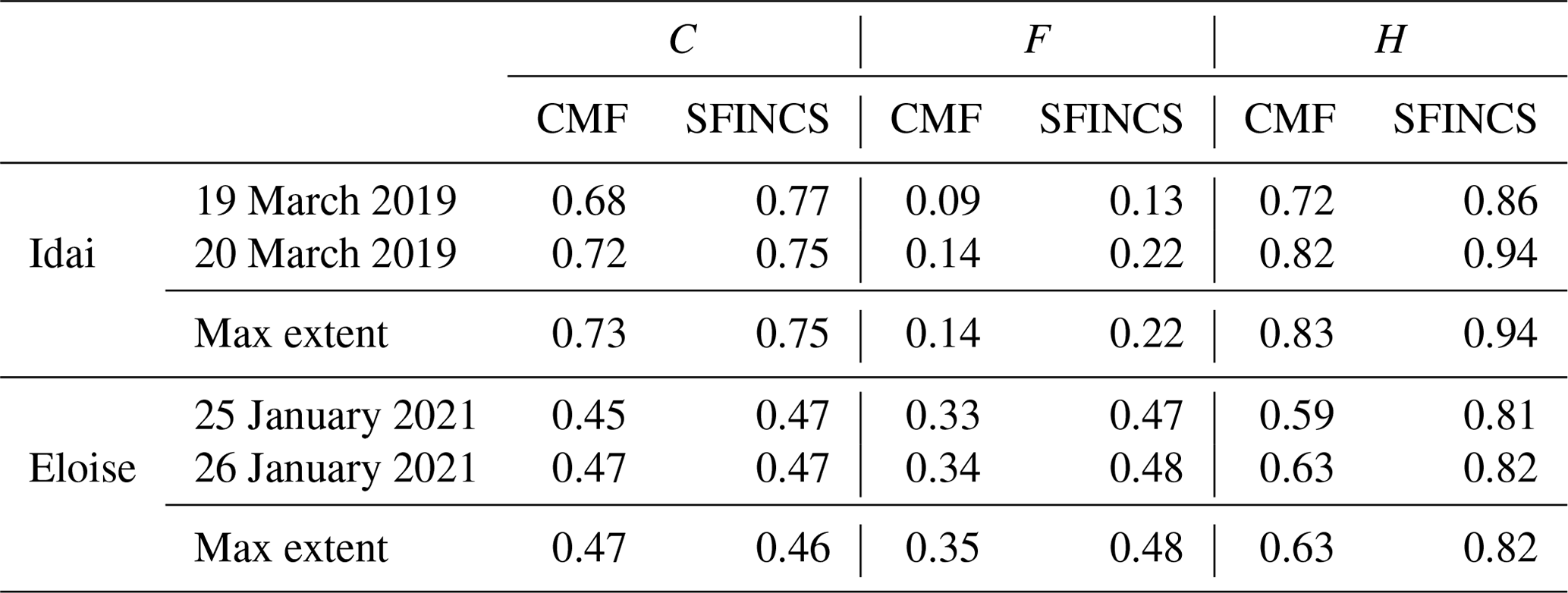
Table 5 Sensitivity analysis of model skill for CaMa-Flood (CMF) and SFINCS (SF) to river depth, Manning roughness, coastal driver (H forcing), pluvial and fluvial drivers (P & Q forcing), bifurcations, and spatial resolution. The model skill is evaluated in terms of the critical success index (C), hit rate (H), and false-alarm ratio (F) based on a comparison of the multi-day maximum simulated and satellite-derived flood extents. For scenarios 1–6 the difference in skill relative to the base scenario is shown; the largest absolute differences per column are highlighted in bold.

4.2 Potential application: compound flood drivers

To showcase a possible application of the compound flood model framework and the added value over the global model, we examine the role of each driver and interactions between flood drivers for both events (Fig. 7). The difference in maximum water levels between the compound scenario and the single-flood-driver scenario that results in the largest flood depth (i.e., the dominant flood driver) is shown in the top panels. The bottom panels show the dominant flood driver with green (pluvial), purple (fluvial), or orange (coastal) colors, which are darker for transition zones, where interactions between drivers amplify the total water level (i.e., show a positive difference in the top panels larger than 5 cm). For most of the model domain, the dominant flood driver during both events is fluvial, especially around the Buzi River and the upstream part of the Pungwe River. The coastal flood driver is dominant in the most downstream ends of both estuaries and in small coastal areas around Beira. Pluvial drivers are dominant on the hillslopes in the northeast corner of the model domain but mainly add to fluvial- and coastal-driven flooding. When we compare both events, we find that the extent where the coastal driver is dominant and the amplification of water levels in the transition zones are larger for Eloise compared to Idai. This can be explained by the difference in fluvial flood magnitude and the timing between the peaks of fluvial and coastal drivers. During Idai, coastal water levels peaked around 15 March, followed by a discharge peak at the Buzi River 3 d later and the Pungwe River 5 d later (Fig. 3, left panels), causing little interaction between the fluvial and coastal drivers. During Eloise, a first discharge peak at the Buzi River occurred 2 d before the coastal water level peak on 23 January, followed by a small peak in the Pungwe River 1.5 d later and another large peak in the Buzi River 3 d later (Fig. 3, right panels), causing a large (>0.2 m) amplification of the water levels in both rivers. We also investigate the sensitivity of the transition zone for river and estuarine bathymetry. For the simulation with deeper bathymetry (scenario 1b in Table 5), the area where the coastal driver is dominant as well as the transition zone in the Pungwe estuary extends a bit further inland (Fig. A4). While these changes are relatively small, the accuracy of the river and estuarine bathymetry is clearly important to accurately determine the transition zone.

Compared to earlier research that focused on interactions between coastal and pluvial drivers (Bilskie and Hagen, 2018; Gori et al., 2020b), we derive transition zones based on three drivers and distinguish between the fluvial and pluvial drivers. In line with the aforementioned studies, our results also demonstrate that a single map with discrete transition zones for a specific region does not exist. A comprehensive overview of flood transition zones could be derived based on the occurrence of compounding effects across a large range of plausible events. The relative timing between peaks of different flood drivers as well as their magnitude has a large effect on the locations and area of transition zones. This is also underlined by a recent study that found that compound flood levels are sensitive to the timing between flood peaks, especially for events and locations where the duration of discharge peaks is relatively short (Harrison et al., 2021).

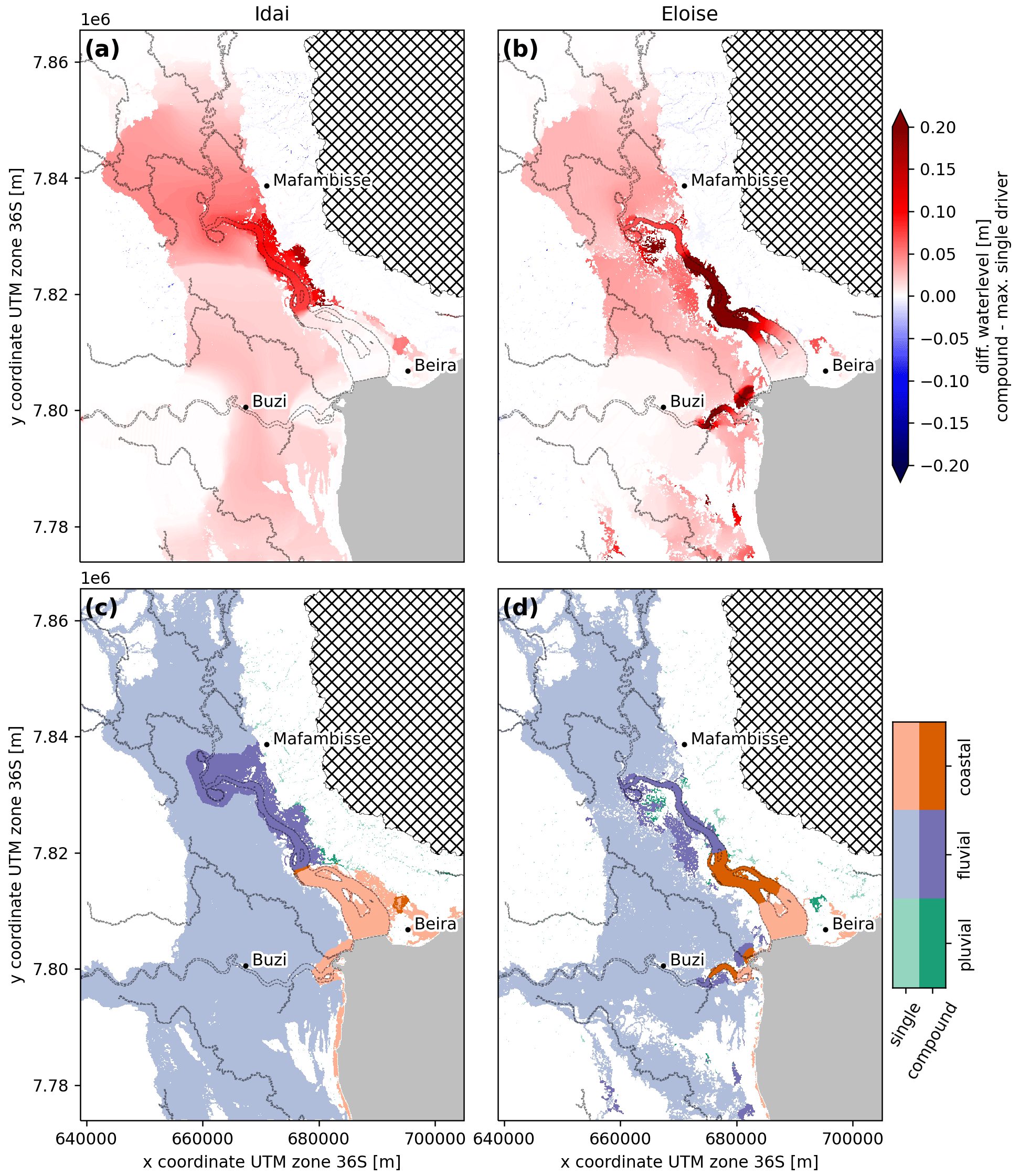
Figure 7 Compound flood dynamics during Tropical Cyclone Idai (a, c) and Tropical Cyclone Eloise (b, d) illustrated by the difference between water levels from the compound flood scenario and the maximum of all single-driver scenarios (a, b) and the main flood driver based on the single-driver scenario with the maximum water level (c, d). The main driver is indicated with light colors where the water level results from a single flood driver and dark colors where it results from more than one flood driver, also referred to as the transition zone.

4.3 Limitations and recommendations

While the presented model framework based on global open-source datasets comes with large benefits in terms of global applicability, the accuracy of the input data is an important consideration. River and estuarine bathymetry is a relatively large source of uncertainty in the current model setup. As bathymetry cannot be directly observed remotely, it needs to be approximated in data-scarce areas where no local measurements are available. This approximation can have a large effect on the result of (compound) inundation simulations (Harrison et al., 2021; Neal et al., 2012; Sampson et al., 2015). Better methods to estimate bathymetry, such as the recently published gradually varying flow theory-based method (Neal et al., 2021; Garambois and Monnier, 2015), and new data, such as expected from the Surface Water and Ocean Topography (SWOT) mission (Andreadis et al., 2020), are expected to be useful to further reduce this uncertainty. For streams smaller than the model resolution, a subgrid schematization could further improve the model (Neal et al., 2012; Volp et al., 2013). A subgrid schematization has recently been implemented in SFINCS (Leijnse et al., 2021) and has been applied by Röbke et al. (2021) for tsunami flood modeling. Furthermore, uncertainties in the global DEM (Hawker et al., 2018a; Hinkel et al., 2021) and the absence of information on flood defense structures in many areas (Scussolini et al., 2016; Wing et al., 2019) may have large implications for the accuracy of the flood simulations. The framework is set up such that datasets can easily be replaced by better (local) datasets, which also facilitates the update of new datasets in future model versions, such as the recently published FABDEM, which is a bias-corrected version of the 30 m resolution Copernicus DEM where the error from vegetation and buildings is reduced (Hawker et al., 2022).

Forcing data are an important source of uncertainty for flood modeling in ungauged areas (Hoch et al., 2019; Wing et al., 2020). For the selected case study, ground observations are very scarce and comparisons with simulated discharge and total sea levels are conducted qualitatively; see Sect. 3.3.1. We recommend investigating whether remote sensing, e.g., satellite laser or radar altimetry data, can be used to validate extreme inland and nearshore water levels (Andreadis et al., 2020; O'Loughlin et al., 2016; Urban et al., 2008). Furthermore, the flood extents derived from Sentinel-1 satellites are known to have limitations in observing obstructed flooding such as in wetland or urban areas (Yang et al., 2021). To further increase the credibility of the model, it should be validated against a larger set of flood events, for instance using the recently published Global Flood Database based on MODIS data (Tellman et al., 2021) or the RAPID Sentinel-1 database over the continental United States (Yang et al., 2021), as well as ground observations.

Furthermore, both events are characterized by a large significant height of wind waves (wave setup component amounts to 24.4 % for Idai and 16.3 % for Eloise of total water levels), indicating that wave setup could not be ignored. In this study we used a simple approach to estimate wave setup, justified by our aim to make the framework globally applicable. The wave setup component could potentially be improved using alternative methods which use additional wave and morphological parameters (e.g., Stockdon et al., 2006), possibly in combination with a recently published dataset on nearshore slopes (Athanasiou et al., 2019). The large computational costs of wave models due to the high spatiotemporal resolution required still prohibits their direct application on large spatial scales (Hinkel et al., 2021). However, these models can still be leveraged for large-scale flood risk applications by developing large synthetic databases of model results for many different plausible cross sections under varying forcing conditions (van Zelst et al., 2021; Pearson et al., 2017). Finally, depending on the wind direction and orientation of the estuary, wind shear can have a significant (but often local) effect on flood levels in coastal environments and can be modeled with SFINCS (Leijnse et al., 2021; Sebastian et al., 2021). This potential driver of compound flooding in coastal environments should be considered in future studies.

5 Conclusions

In this study, we presented an automated framework to model compound flooding anywhere on the globe in a reproducible and transparent manner, and we evaluated its suitability and use for identifying compound flood drivers. The framework is comprised of the high-resolution 2D flood model SFINCS, set up based on global datasets and forced by global models at its boundaries. For two historical compound flood events in the Sofala province of Mozambique, we compared the skill of the globally applicable flood model with the global quasi-2D CaMa-Flood model. The validation against flood extents from satellites shows a good model performance. The SFINCS model shows slightly better skill than CaMa-Flood in terms of the critical success index, but large differences exist in the simulated flood maps. Firstly, the globally applicable model can accommodate for direct coastal and pluvial flooding as well as interactions between coastal, pluvial, and fluvial drivers, thereby providing a more comprehensive description of flooding in coastal deltas than the global model, resulting in a higher hit rate. Secondly, while the multiple downstream connectivity (or bifurcation) scheme largely improves the results of the global model, the floodplain connectivity is still limited, resulting in higher flood levels and smaller flood extents. Thirdly, pluvial flooding is likely overestimated in the globally applicable model as small streams are not represented in the model, thus underestimating the drainage capacity. We hypothesize that this will improve with the recently implemented subgrid schematization in SFINCS in combination with higher-resolution DEMs. Finally, we showed that the globally applicable model can be used to analyze the effect of interactions between flood drivers, here for the first time presented with joint fluvial, pluvial, and coastal flood drivers. We found that the transition zones between flood drivers vary significantly between flood events due to differences in the relative timing between and magnitude of each driver. As the identification of these zones is important to understand flood preparedness and response, their identification should therefore be based on a large number of plausible flood events. We also reiterate the importance of observed water levels for a more comprehensive comparison of flood simulations.

The automated model setup is available through the open–source Python package HydroMT-SFINCS and allows for a fast and reproducible setup of compound flood hazard models. With sufficient computational resources, the framework therefore has the potential to be scaled up to large spatial scales by setting up many high-resolution models in river and coastal floodplains but could also rapidly be employed for disaster response.

Appendix A: Supporting figures

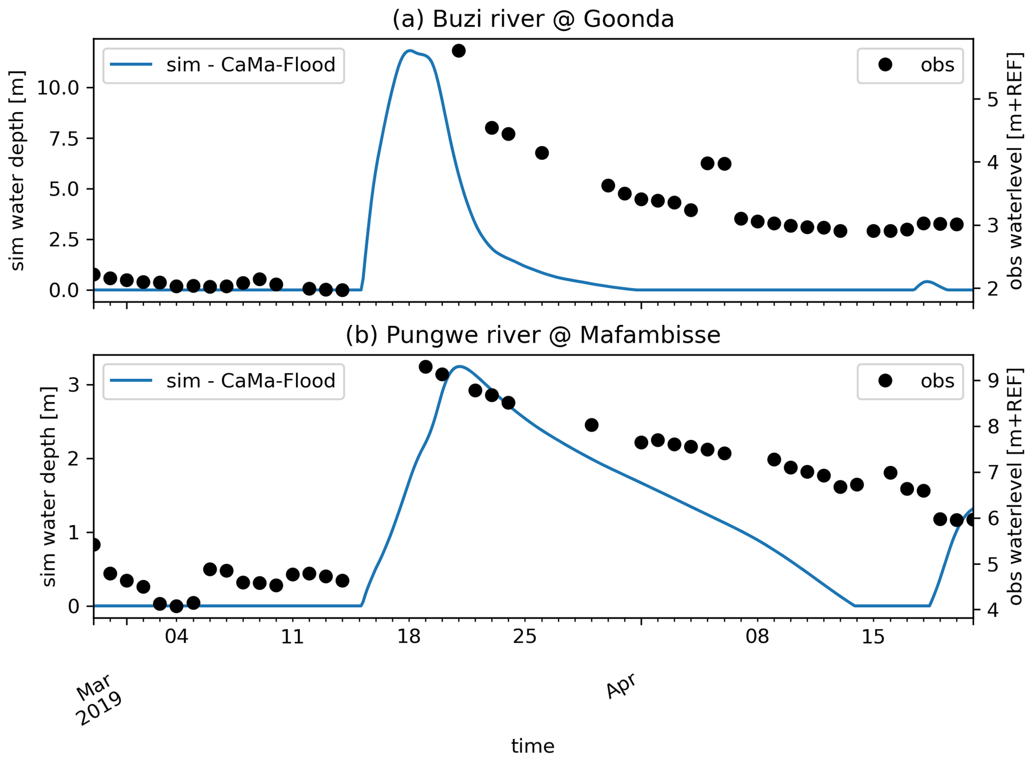
Figure A1 Comparison of observed water levels and simulated water depths during Tropical Cyclone Idai in the Buzi (a) and Pungwe (b) rivers. Note that the comparison is based on approximate locations as the precise locations could not be retrieved. Furthermore, as the vertical datum of the observations is unknown, these are plotted on a second y axis.

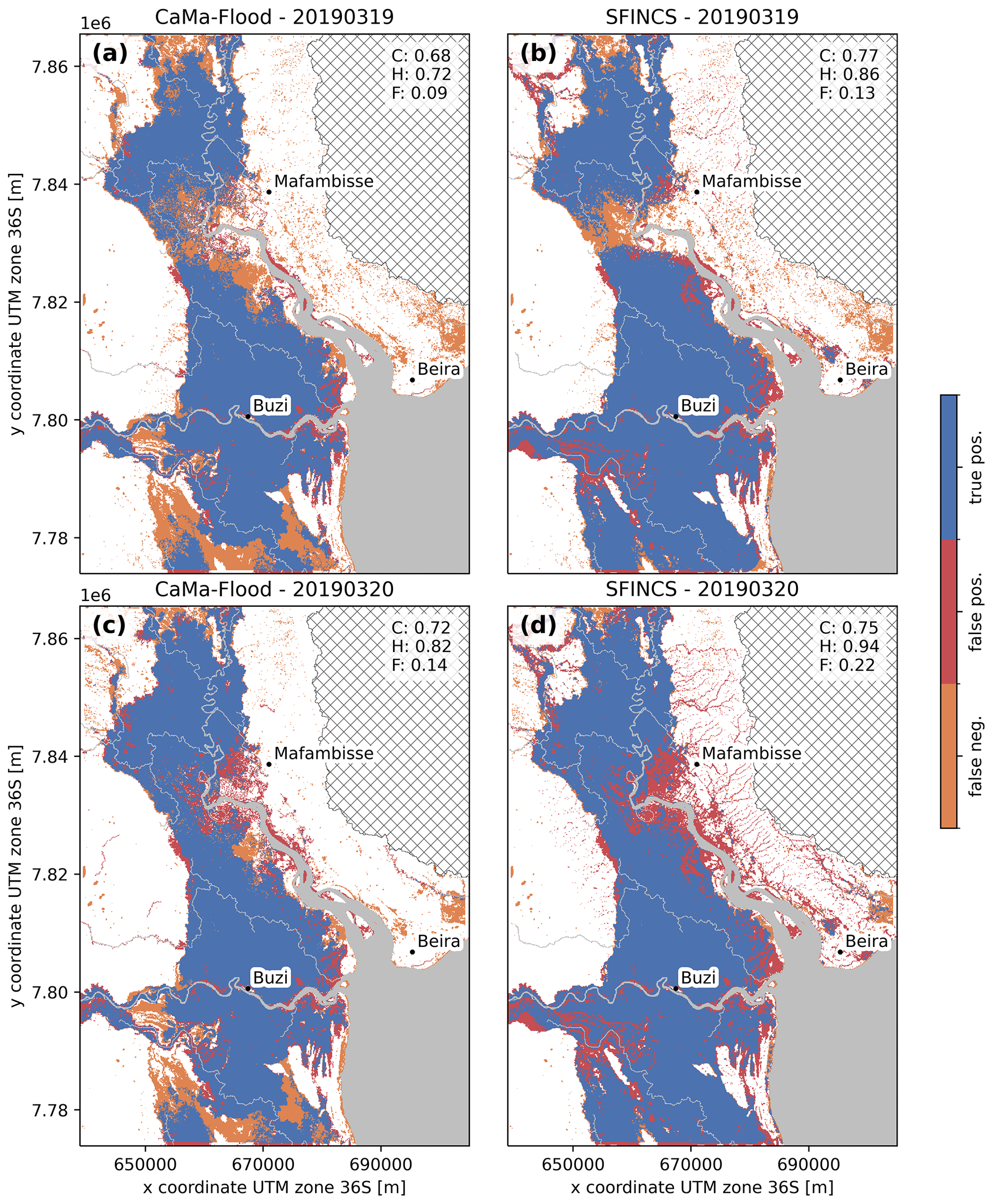
Figure A2 Simulated maximum flood depths from CaMa-Flood (a, c) and SFINCS (b, d) for Tropical Cyclone Idai on 19 March (a, b) and 20 March (c, d). The grey areas indicate permanent water, and the hatched areas are excluded.

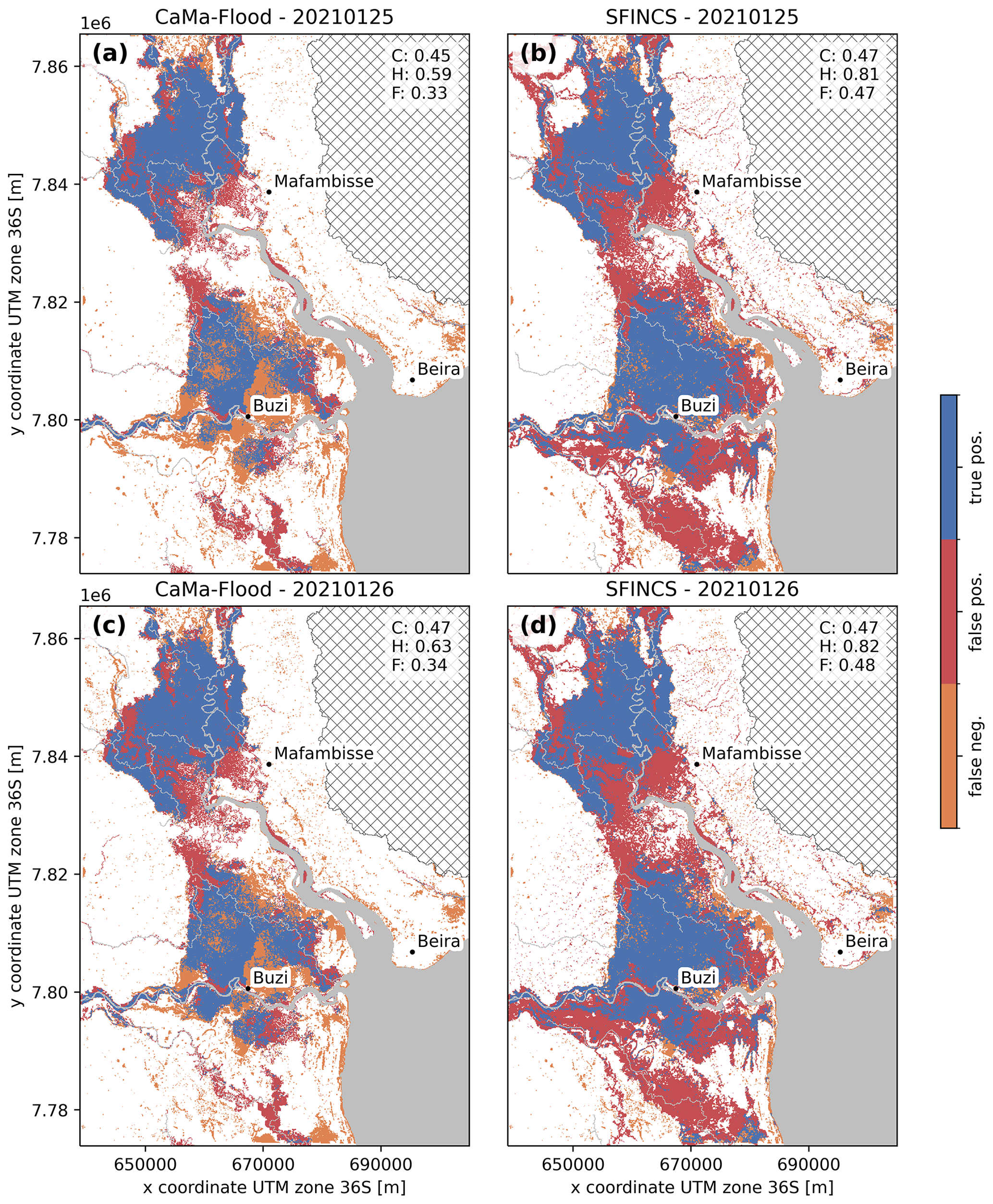
Figure A3 Simulated maximum flood depths from CaMa-Flood (a, c) and SFINCS (b, d) for Tropical Cyclone Eloise on 25 January (a, b) and 26 January (c, d). The grey areas indicate permanent water, and the hatched areas are excluded.

Figure A4 Sensitivity analysis of compound flood dynamics simulation based on 150 % river depth during Idai (a, c) and Eloise (b, d) illustrated by the difference between water levels from the compound flood scenario and the maximum of all single-driver scenarios (a, b) and the main flood driver based on the single-driver scenario with the maximum water level (c, d). The main driver is indicated with light colors where the water level results from a single flood driver and dark colors where it results from more than one flood driver, also referred to as the transition zone.

Appendix B: HydroMT configuration

Figure B1 Example HydroMT-SFINCS configuration file used to set up the SFINCS model schematization (see Sect. 3.2.1). Each section corresponds to a step in the automatic model-building process. Options ending with _fn (filename) correspond to data from the data catalog; see Table B2.

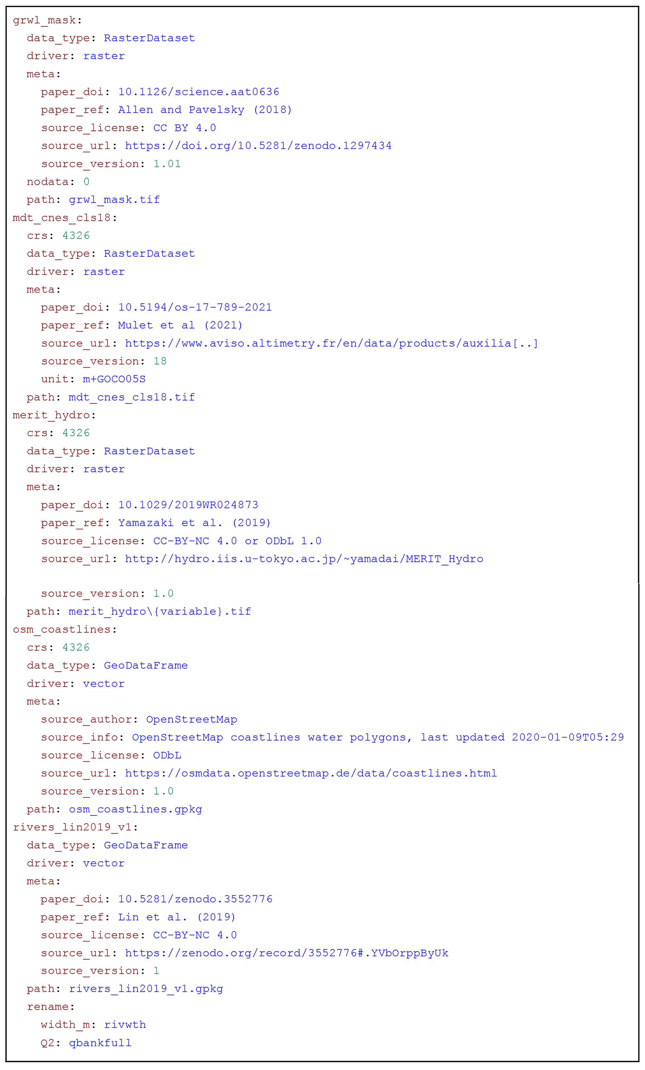
Figure B2 Data catalog (.yaml) file used to set up the SFINCS model schematization (see Sect. 3.2.1). Each entry corresponds to a dataset and contains information about how to read it and which preprocessing steps (such as renaming) are required.