the Creative Commons Attribution 4.0 License.
the Creative Commons Attribution 4.0 License.
 | 21 Jul 2023
Trends in heat and cold wave risks for the Italian Trentino-Alto Adige region from 1980 to 2018
Martin Morlot
Simone Russo
Luc Feyen
Giuseppe Formetta
Heat waves (HWs) and cold waves (CWs) can have considerable impact on people. Mapping risks of extreme temperature at local scale, accounting for the interactions between hazard, exposure, and vulnerability, remains a challenging task. In this study, we quantify risks from HWs and CWs for the Trentino-Alto Adige region of Italy from 1980 to 2018 at high spatial resolution. We use the Heat Wave Magnitude Index daily (HWMId) and the Cold Wave Magnitude Index daily (CWMId) as the hazard indicators. To obtain HWs and CW risk maps we combined the following: (i) occurrence probability maps of the hazard obtained using the zero-inflated Tweedie distribution (accounting directly for the absence of events for certain years), (ii) normalized population density maps, and (iii) normalized vulnerability maps based on eight socioeconomic indicators. The methodology allowed us to disentangle the contributions of each component of the risk relative to total change in risk. We find a statistically significant increase in HW hazard and exposure, while CW hazard remained stagnant in the analyzed area over the study period. A decrease in vulnerability to extreme temperature spells is observed through the region except in the larger cities where vulnerability increased. HW risk increased in 40 % of the region, with the increase being greatest in highly populated areas. Stagnant CW hazard and declining vulnerability result in reduced CW risk levels overall, except for the four main cities where increased vulnerability and exposure increased risk levels. These findings can help to steer investments in local risk mitigation, and this method can potentially be applied to other regions where there are sufficient detailed data.
- Article
(4298 KB) - Full-text XML
-
Supplement
(927 KB) - BibTeX
- EndNote


Heat waves (HWs) and cold waves (CWs) are hazards that affect public health and the environment (Gasparrini et al., 2015; Habeeb et al., 2015). With global warming, HW intensities and durations are expected to increase, while those of CWs are expected to decrease (Perkins-Kirkpatrick and Gibson, 2017; Russo et al., 2015; Smid et al., 2019), changing the risks they pose to society. A recent report showed that in the year 2018 worldwide, 157 million more people were exposed to HWs compared to the year 2000 (Watts et al., 2018). In Europe, recent high-intensity HW events (2003 and 2018) – where HWs are defined as 3 d over 90th temperature percentile of the 1980–2010 – have impacted as much as 55 % of its area (García-León et al., 2021). In Italy, HWs had a strong impact on mortality. For example, in 2003, a 27 % mortality increase was reported over August compared to August 2002; there was also a 23 % increase in July 2015 compared to the same month for the 5 previous years (Michelozzi et al., 2005, 2016). In Trentino-Alto Adige (our study region), Conti et al. (2005) showed that the large HW of 2003, compared to the previous year, increased mortality by 32 % in Trento and 28 % in Bolzano (the region's two main cities). In the city of Bolzano, it was found that higher hospital admissions occurred during HW events, particularly among elderly women (Papathoma-Köhle et al., 2014). With regards to CWs in Europe, recent winters have claimed lives with 790 deaths in 2006 and 549 deaths in 2012 (Kron et al., 2019). In Italy, de'Donato et al. (2013) report an increase in mortality (47 %) for the time frame of the 2012 CW in the city of Bolzano compared to the four previous winters (2008–2011).
HW and CW events clearly drive risk, but how do we define this risk? The United Nations Office for Disaster Risk Reduction (UNDRR, 2021) and the Intergovernmental Panel on Climate Change (IPCC, 2014) define risk as a function of hazard, exposure, and vulnerability. Hazard is defined as a process, phenomenon, or human activity that may cause loss of life, injury, or other health impacts; property damage, social and economic disruption; or environmental degradation and hazards characterized by location, intensity or magnitude, frequency, and probability. Exposure is defined as people, infrastructure, housing, production, and other tangible human assets present in hazard-prone areas. Vulnerability is defined as the conditions that define the susceptibility of an individual, infrastructure, or a community to be impacted by the hazard. To successfully quantify risk, one must measure all three components: hazard, exposure, and vulnerability.
With regard to temperature-related hazard and exposure, several studies have been conducted at global (e.g., Chambers, 2020; Dosio et al., 2018), continental (e.g., King et al., 2018), and at city scale (e.g., Smid et al., 2019). Most studies focus on human exposure (e.g., Chambers, 2020; Tuholske et al., 2021) and on the exposure of different land areas (e.g., Ceccherini et al., 2017; van Oldenborgh et al., 2019; Russo et al., 2016). These studies find increasing trends in HW (Chambers, 2020; Dosio et al., 2018) and decreasing trends in CWs in their period of analysis (van Oldenborgh et al., 2019; Smid et al., 2019).
Studies on HWs and CWs typically have used subjective numerical thresholds, on the indicator to define severity and exposure to the hazards (e.g., 0<HWMId<3, 3<HWMId<6, 6<HWMId<9, where HWMId is Heat Wave Magnitude Index daily). However, extreme events are usually defined by their return periods. In the case of HWs and CWs, fitting extreme value distributions to define the return periods is difficult due to the possible absence of events in the analyzed time frame (i.e., zero values, in the case where there are no HWs or CWs in a given year). Generalized extreme value distribution (GEV) and non-stationary techniques (Dosio et al., 2018; Kishore et al., 2022; Russo et al., 2019) have enabled estimation of HW and CW return periods, but neither approach explicitly accounts for a zero presence in an analyzed time series.
In this study, for the first time, we use a distribution allowing for the direct fitting of zero values for extremes (years with no event): the zero-inflated distribution of Tweedie families (Jorgensen, 1987; Tweedie, 1984). This distribution is also used to estimate HW and CW frequency of occurrence. The Tweedie distribution has been used mostly for the purpose of the analysis of insurance claims. It has seldom been applied in the field of natural hazards, such as HW mortality (Kim et al., 2017), drought (Tijdeman et al., 2020), or rainfall analysis (Dunn, 2004; Hasan and Dunn, 2011). The main advantage of the Tweedie distribution is the possibility of considering a range of distributions to describe continuous and semi-continuous domains; these include normal, gamma, Poisson, compound gamma–Poisson, and inverse Gaussian (Bonat and Kokonendji, 2017; Rahma and Kokonendji, 2022; Shono, 2008; Temple, 2018). Moreover, for some of these distributions (i.e., Poisson mixtures of gamma distributions), the Tweedie distribution approach explicitly enables the fitting of zero-inflated data. The distribution's main limitation is the complex distribution's fitting methodology and the difficulties in obtaining relevant information criteria, such as Akaike's information criterion (Shono, 2008). The implication of these limitations is that the “fitting” of the Tweedie distribution is computationally intensive and that it is difficult to compare its goodness of fit to other distributions via the information criterion.
To perform any risk analysis, vulnerability to the hazard must be quantified. HW and CW vulnerabilities can be approximated though the combinations of several socioeconomic indicators. Cheng et al. (2021) provide an overview of the different types of indicators used in the literature to quantify vulnerability. The indicators can be diverse, ranging from population structure (e.g., age and health characteristics), social status, economic conditions, community (cultural) group characteristics, and household physical characteristics. At the community level in the United States, indicators such as social isolation, presence of air conditioning, proportion of elderly, and proportion of diabetics in the population have been found to be key for human vulnerability to temperature extremes (Reid et al., 2009). At the national level in South Korea, Kim et al. (2017) found that elderly living alone, agricultural workers, and the unemployed are the main indicators of vulnerability to heat wave days and tropical nights. Vulnerability indicators, in combination with temperature–mortality relationships, have also been appraised at city scale for HWs (Ellena et al., 2020) and at regional scale (López-Bueno et al., 2021) for CWs (Karanja and Kiage 2021). A study on social vulnerability to natural hazards in Italy (Frigerio and De Amicis, 2016) used seven indicators (i.e., family structure, education, socioeconomic status, employment, age, race and ethnicity, and population growth) derived from the freely available census records.
HW and CW risks overall are often assessed using different methodologies depending on the objectives of the study. On a global scale, Russo et al. (2019) establish a risk index using the probabilities of HWs as hazard, where the exposure is the population density normalized in [0;1] based on its maximum and minimum values, while vulnerability is based on a socioeconomic indicator (human development index). For Italy, Morabito et al. (2015) conducted a risk analysis of heat on elderly in the major cities, using the elderly population as the only vulnerability factor and summer average temperatures for the period 2000–2013 to quantify hazards.
In this study, we assess risk associated with extreme temperatures in the Italian Trentino-Alto Adige region. This is a relevant social and scientific objective given (i) the increase in the percentage of elderly people (i.e., vulnerability change) (Papathoma-Köhle et al., 2014) and (ii) changing temperature extremes in view of climate change (i.e., changing hazard). Few studies have attempted to quantify HW and CW impacts for the cities of Trento and Bolzano (main cities of the region), including Conti et al. (2005) as part of their studies on Italian cities and Papathoma-Köhle et al. (2014), who studied impacts in Bolzano. The former compared mortality data of the year 2003, when there was a very intense HW, to the year 2002, finding an increase of mortality in both Trento and Bolzano. The latter compared hospital admissions due to HWs in summer months of 3 years (2003, 2006, and 2009) and found heat health-related issues driving admissions among elderly women.
To understand the evolution of HW and CW human risk and to plan adequate risk-mitigation measures in the region of study, the risk and its change at high spatial and temporal resolution need to be analyzed. The aim of this research is to improve quantification of HW and CW hazards, human exposure, vulnerabilities, over the period 1980–2018, for the Trentino-Alto Adige region to better assess related risks at high definition (i.e., city scale). The goals for this paper are therefore as follows:
-
quantify HW and CW hazards and their return level at a very high spatial resolution (250 m) by combining for the first time (i) the indicators proposed (HWMId, CWMId – Cold Wave Magnitude Index daily) by Russo et al. (2015) and Smid et al. (2019), together with (ii) the Tweedie distribution;
-
quantify human exposures and vulnerabilities to HWs and CWs and their evolution over time for the Trentino-Alto Adige region;
-
quantify HW and CW risks across the region and understand their main drivers, disentangling how their individual components drive these risks over time.
The Trentino-Alto Adige region (Fig. 1) is a mountainous region in northern Italy, which borders Austria. The elevation of the region varies from 65 m for Lake Garda to 3905 m for the Ortler. It is composed of two provinces (Province of Trento and Province of Bolzano). Its most populous cities (population for 2022 in parentheses) are the two provincial capitals, Trento (118 509) and Bolzano (107 025), as well as minor cities such as Merano (40 994) and Rovereto (39 819). The main rivers in the region are the Adige and its tributary, the Isarco. Due to its diverse geography, the climate is also diverse, ranging from subcontinental to alpine according to the Köppen classification (Fratianni and Acquaotta, 2017).
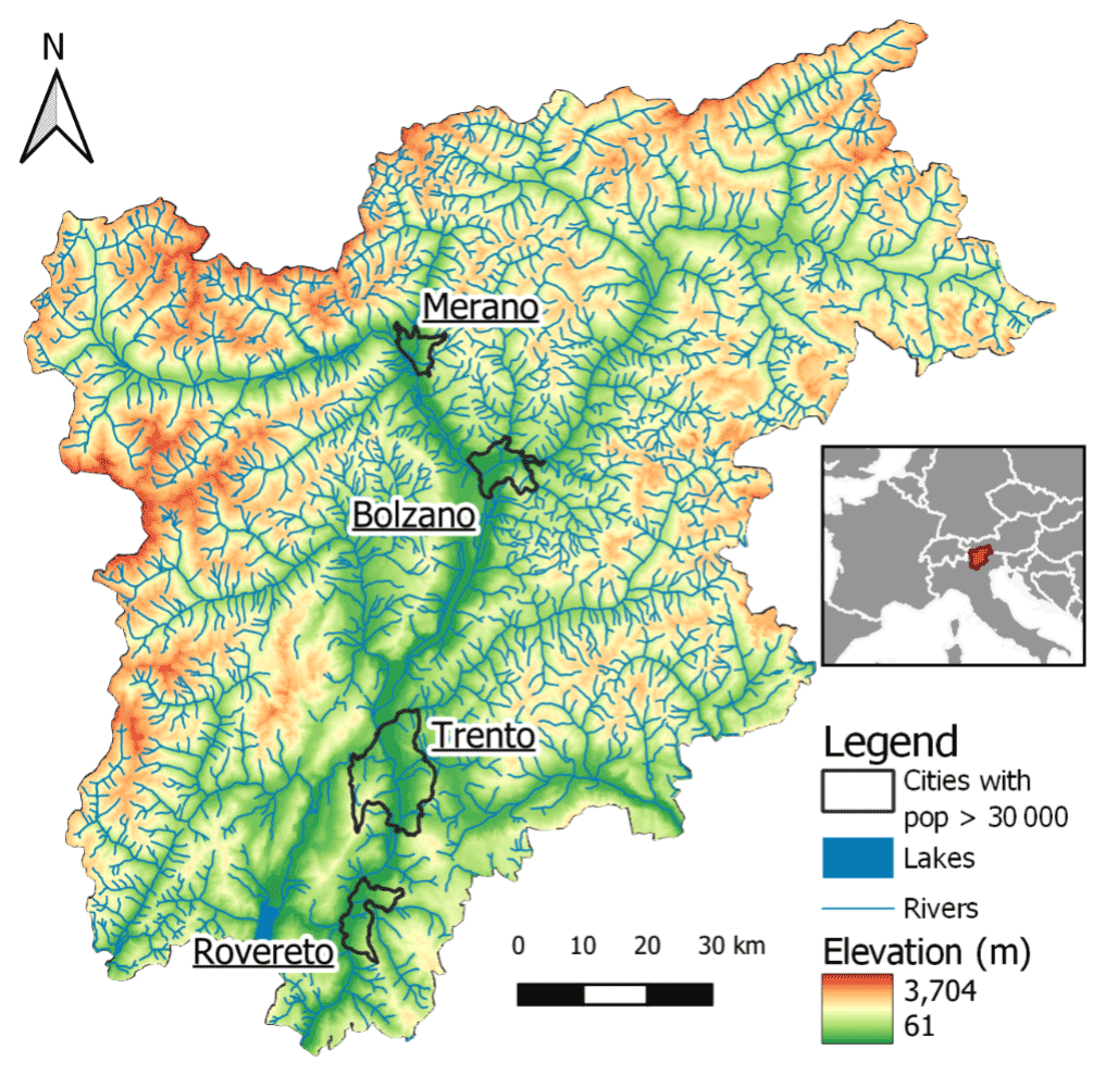
Figure 1The Trentino-Alto Adige region and its most populated cities (Trento, Bolzano, Rovereto, and Merano); the colors indicate the elevations, river network, and lakes.
3.1 Temperature data
In order to quantify the HW and CW hazard, we used the freely available spatial–temporal temperature dataset by Crespi et al. (2021). It consists of gridded daily temperatures for the entire Trentino-Alto Adige region covering the period of 1980–2018 at a resolution of 250 m. The dataset is based on more than 200 station's daily records that have been quality controlled and homogenized. The interpolation method is based on a combination of 30-year temperature climatology (1981–2010) and daily anomalies, and it accounts explicitly for topographic features (i.e., elevation, slope) that are crucial in orographically complex areas like the Trentino-Alto Adige region. The leave-one-out cross-validation presented in Crespi et al. (2021) finds a mean correlation coefficient that is higher than 0.8 and mean absolute errors of around 1.5 ∘C (on average across months and stations used for the interpolation).
3.2 Hazard quantification and distribution fitting
3.2.1 Hazard quantification
To quantify the hazard, we used the HWMId (Russo et al., 2015) and the CWMId (Smid et al., 2019). These indices represent a way of measuring extreme temperature events while considering their durations and intensities and accounting for site-specific historical climatology (30 years).
According to Russo et al. (2015), HWMId is defined as the maximum magnitude of the HWs in a year. A HW occurs when the air temperature is above a daily threshold for more than 3 consecutive days. The threshold is set to the 90th percentile of the temperature data of the day and the window of 15 d before and after, throughout the reference period 1981–2010. The magnitude of a HW is the sum of the daily heat magnitude HMd of all the consecutive days composing the HW (Eq. 1):
where HMd (Td) corresponds to the daily heat magnitude, Td the temperature of the day in question, and T30y25p and T30y75p correspond to the 25th and 75th percentile of the yearly maximum temperature for the 30 years of the reference period (1981–2010). The interquartile range (IQR, i.e., the difference between the T30y75p and T30y25p percentiles of the daily temperature) is used as the heat wave magnitude unit and represents a non-parametric measure of the variability of the temperature time series. Therefore, a value of HMd equal to 3 means that the temperature anomaly on day d with respect to T30y25p is 3 times the IQR. Finally, for a given year HWMId corresponds to the highest sum of magnitude (HMd) over the consecutive days composing a heat wave event (with only days with HMd > 0 considered).
Analogously to the HWMId, CWMId is defined as the minimum magnitude of the CWs in a year (Smid et al., 2019). A CW occurs when the air temperature is below a daily threshold for more than 3 consecutive days. The threshold is set to the 10th percentile of the temperature data of the day and the window of 15 d before and after, throughout the reference period 1981–2010.
The daily cold magnitude corresponds to Eq. (2):
where CMd (Td) corresponds to the cold daily magnitude, Td the daily temperature, and T30y25p and T30y75p correspond to the 25th and 75th percentile yearly temperature for the 30 years used as a reference. Inversely to HWMId, the lowest cumulative magnitude sum is retained for each year and with only consecutive days with CMd < 0 considered to calculate it. CWMId always being < 0, its absolute values are retained for its values to be on a positive interval (similar to HWMId).
3.2.2 Distribution fitting
The HWMId and CWMId yearly values are fitted with a probability distribution to estimate their return periods. Considering that HWMId and CWMId are both defined in [0,+Inf[, we use the Tweedie distribution (Jorgensen, 1987; Tweedie, 1984), a distribution that can act as zero-inflated, thus accounting for the presence of zeros directly. The Tweedie distribution is an exponential dispersion model which has a probability density function of the following form (Eq. 3):
where Φ corresponds to its dispersion parameter that is positive, θ to its canonical parameter, and κ(θ) the cumulant function. The function a(y, Φ) generally cannot be written in closed form. The cumulant function is related to the mean ( and variance (, and in the case of a Tweedie distribution the variance has a power relationship with the mean (Eq. 4):
where p corresponds to the power parameter that is positive.
Depending on the value of p, the distribution will behave differently. In the case where p is between 1 and 2, it belongs to the compound Poisson–gamma distribution with a mass at zero, while other p values can make the distribution correspond to a normal, Poisson, or gamma distribution, among others. The use of the Tweedie distribution is retained, permitting us to consider the zero values while also considering other distributions should there be an absence of zero values.
We fit the distribution to the previously found HWMId and CWMId values with the help of the Tweedie R package (Dunn, 2021). It provides distribution density, distribution function, quantile function, and random generation for the Tweedie distributions. The Tweedie parameters (i.e., mean, power, and dispersion) have been estimated by the “tweedie.profile” function (Dunn, 2021) using the maximum likelihood as described by Dunn and Smyth (2005). An example of the fitted distribution for Bolzano and Trento can be found in the Supplement (Fig. S1 in the Supplement). It is also possible to use the same package to estimate a quantile using the fitted distribution, permitting us to estimate specific return levels for return periods T for both HWMId and CWMId. For this study two return levels are retained: 5 years (HW5Y for HW, and CW5Y for CW) and 10 years (HW10Y for HWs and CW10Y for CW). This choice aims to account for both the length of the analyzed period (39 years) and the type of hazards we are analyzing (HWs and CWs usually do not occur every year). Higher return level estimations would be affected by extrapolation effects and higher uncertainties.
For statistical fit verification, the Kolmogorov–Smirnov (KS) test on two samples is used with one sample being the HWMId or CWMId values and the other sample being a randomly generated sample using the fitted distribution value. This goodness-of-fit test is one of the most commonly used in the literature for zero-inflated Tweedie distribution (Goffard et al., 2019; Johnson et al., 2015; Rahma and Kokonendji, 2022). The null hypothesis of this test is that the two samples belong to the same distribution. If the P value for this test is below the significance level α of 5 %, the null hypothesis is rejected, otherwise we cannot reject the null hypothesis at this significance level.
3.3 Exposure quantification
To quantify the population exposed to HWs and CWs, we use time-varying population data from the Global Human Settlement Layer (GHSL) (Schiavina et al., 2019). The population data are available at a resolution of 250 m for the following years: 1975, 1990, 2000, and 2015. Both these data, as well as the population count done by the Italian national statistical institute, indicate a growing population throughout the region in the period for which data are available (overall 23 %, 1975–2015).
To model more accurately exposure, we created yearly varying population maps for the period 1980–2018, following the methodology presented in other studies (e.g., Formetta and Feyen, 2019; Neumayer and Barthel, 2011). We linearly interpolated the data in time for the period 1980 to 2015 (assuming a constant rate in between available years), and we used the closest year for the period 2016–2018.
Following recent studies (King and Harrington, 2018; Russo et al., 2019), for each year, a pixel is considered exposed to HW/CW hazard (or to a 5- or 10-year return period HWs/CWs) if, for that year, the HWMId/CWMId of the pixel is greater than zero (or greater than the corresponding return level HW5Y/CW5Y or HW10Y/CW10Y, respectively). This is the exposition factor, and it is a binary value (0 meaning unexposed or 1 meaning exposed).
The percentage of population exposed is calculated on an annual basis over the study period (1980–2018) and with the help of population data linearly interpolated from 1980 to 2018.
Using this population data, the percentage of population exposed is then calculated using the following equations (Eqs. 5 and 6):
where i corresponds to the pixels, t to the year being analyzed, and EF to the exposition factor mentioned above (binary).
3.4 Vulnerability quantification
We express HW and CW vulnerability using eight indicators as in Ho et al. (2018); they quantify community vulnerability to HW and CW events based on extreme age, household physical characteristics, social status, and economic conditions. The list of variables considered is reported in Table 1.
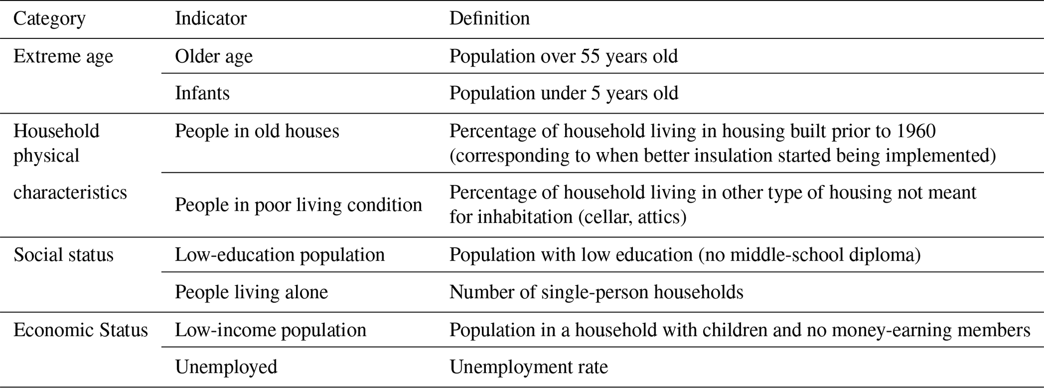
The spatially varied indicators are freely available in the census records (i.e., sub-city level) from the Italian national statistical institute (ISTAT, 2021) for 3different years (1991, 2001, 2011). Given the data time constraints, vulnerability is thus derived for these 3 years only.
The methodology to quantify vulnerability uses the equal weight analysis (EWA; e.g., Liu et al., 2020). Firstly, the individual indicators are standardized between 0 and 1, prior to aggregation (their sum); the standardization is done at the city level for the 3 years of record (1991, 2001, 2011) based on Eq. (7):
This approach was chosen as it is the simplest method for weighing the vulnerability indicators, and it is commonly applied in the literature with regards to HWs and CWs (e.g., Buscail et al., 2012; Buzási, 2022).
Finally, we created yearly varying vulnerability maps for the period 1980–2018 following the same linear interpolation approach used for the population.
3.5 Risk quantification
Risk is a function of hazard, exposure, and vulnerability, multiplied to quantify risk (UNDRR, 2021). This is one of the two most commonly used approaches in the literature (Dong et al., 2020; Quader et al., 2017; Russo et al., 2019), with the other approach being the addition of the different risk components. Multiplication when compared to addition is found to better highlight the complex relationship between the different components, due the multiplication of the multivariate probabilities of independent variables following a product law (El-Zein and Tonmoy, 2015; Estoque et al., 2020; Peng et al., 2017).
The risk is calculated as per Dong et al. (2020) (Eq. 9):
with each of the risk components having a value in [0,1]. The hazard is computed as the probability of occurrence of HWs/CWs using the fitted Tweedie distribution probability function for each pixel. Exposure is the standardized population density. The vulnerability derived from standardized variables is also between [0,1]. The resulting risk is therefore bound by 0 and 1, with 0 corresponding to the lowest level of risk and 1 to the highest level of risk.
The risk is calculated at the municipality level because it is the lowest level of resolution of the three elements that compose it.
In order to further investigate which are the driving factors of the risk, we disentangle the marginal effect of each component (i.e., hazard, exposure, and vulnerability) for both HWs and CWs. In turn, one of them is allowed to vary across 1980–2018 and two of them are kept constant (to their value at the year 2003, the middle of the analyzed period).
3.6 Trend analysis and statistical significance
The trends are analyzed using the robust regression technique (Huber, 2011) which is often used to assess trends in natural hazards (Formetta and Feyen, 2019 for multiple hazards and Kishore et al., 2022, specifically for HWs). Robust regression seeks to overcome part of the limitations of traditional regression analysis.
For example, the linear regression least squares method is optimal when the regression's assumptions (normal distribution, independence, equal variance) are valid (Filzmoser and Nordhausen, 2021; Khan et al., 2021). This method can be sensitive to outliers or if normality is dissatisfied (Khan et al., 2021; Brossart et al., 2011). The robust regression method is designed to limit the effect that invalid assumptions have on the regression estimates (Filzmoser and Nordhausen, 2021; Alma, 2011).
To confirm the statistical significance of the trends, the false discovery rate (FDR) methodology is used according to Wilks (2016) and Leung et al. (2019), with a significance level α=0.05. The FDR is defined as the statistically expected fraction of null hypothesis test rejections at the grid cell for which the respective null hypotheses are true (Wilks, 2016).
4.1 Hazard quantification and trends
For HW hazard intensities, the most notable year on record (1980–2018) in the region is 2003, where HWMId reached a pixel maximum of 30.4 and a median value of 16.9 over the area (Fig. 2). The second most intense HW occurred in 2015 and the third most intense in 1983. Out of the 6 years with the highest median HWMId between 1980 and 2018, 4 years occurred in the last decade (2010, 2013, 2015, 2017), suggesting that climate change is already increasing the frequency of heat waves in the Trentino-Alto Adige region. For CW, only 1985 stands out, with a maximum and median CWMId of 27 and 14.5, respectively, or nearly 3 times more than that of any other year on record. The second strongest cold wave occurred in 2012.
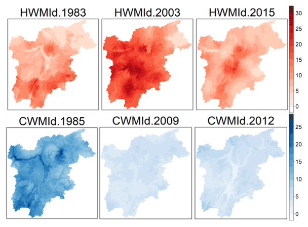
Figure 2Regional Heat Wave Magnitude Index daily (HWMId) and Cold Wave Magnitude index daily (CWMId) maps for single years with the highest regional average on record (1980–2018).
The KS test p values (Fig. S2 in the Supplement) indicate that the fitting of the Tweedie distribution with power parameter values between [1,2] cannot be rejected for both HWMId and CWMId. This enables us to estimate return levels for both HWs and CWs and analyze trends based on them. The return levels for return periods of 5 years (HW5Y, CW5Y) and years (HW10Y, CW10Y) for every pixel are shown in Fig. S3.
Fitting the robust linear model to the HW values, statistically significant positive trends are found for HWs (i.e., HWMId > 0) and HWs with a magnitude larger than the 5-year event (HWMId > HW5Y) in most pixels of the region (Fig. 3). For rarer events, those larger than the 10-year event (HWMId > HW10Y), no statistically significant increase in HW intensity is found in the region. Regarding location of these trends, some of the highest elevation parts of the region have the greatest coefficient of increase (i.e., north of Bolzano and in the mountains located in the northwest of the region). For all CWs, we do not find statistically significant trends in any part of the region.
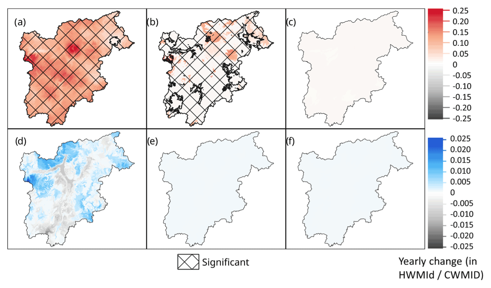
Figure 3Trends in heat waves (HWs) and cold waves (CWs) using the robust linear model based on yearly HWMId and CWMId magnitudes from 1980 to 2018 for HWs (a) with HWMId > 0, (b) with HWMId > HW5Y, (c) HWMId > HW10Y and for CWs and (d) with CWMId > 0, (e) with CWMId > CW5Y, (f) CWMId > HW10Y.
4.2 Population exposure
Summing the overall number of people exposed over intervals (i.e., one person can be exposed each year and therefore counted multiple times over the interval), between 1980 and 2000 in the study region, about 900 000 people were exposed to a 5-year HW event, 250 000 to a 10-year HW event, 3 million to a 5-year CW event, and 1.9 million to a 10-year CW event. More recently, between 2000 and 2018, the population exposure values increased significantly to over 5 million for a 5-year HW event and to about 2.5 million for a 10-year HW event, but the numbers decreased for CW events, to 2.4 million for a 5-year CW event and to 500 000 for a 10-year CW event. Due to the importance of the demographic change in the region over the full study period (increase of population by 23 %), it is important to analyze the percentage of population impacted by these different events. This will help us to disentangle what is driving these changes, e.g., whether these changes are due to demographic changes or to the change in the frequency of events or both.
Figure 4 presents the share of the population exposed to HW and CW intensities larger than those of 5-year and 10-year events over the period 1980 to 2018 on a yearly basis. It shows that a higher share of the population was exposed to HWs more frequently after 2000 compared to the first 2 decades (1980s and 1990s). For both return periods, the robust linear model indicates a significant increase in the share of the population exposed to HWs across the region, with a coefficient for the increase of nearly 1 % per year for HWs > HW5Y and 0.02 % for HWs > HW10Y. We did not find a significant trend in human exposure to CWs in the region.
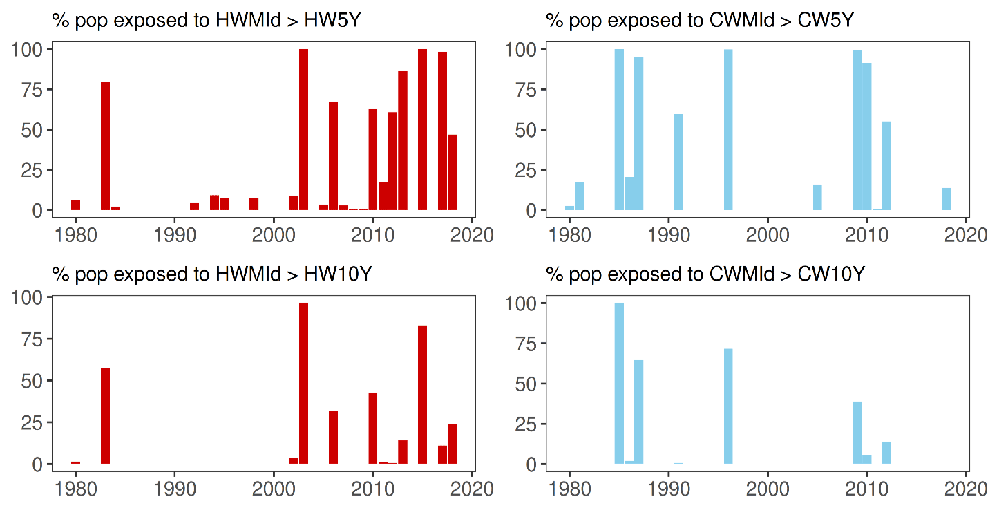
Figure 4Percentage of population exposed to heat wave and cold wave events greater than the return levels of 5 and 10 years over the span of 1980–2018.
4.3 Vulnerability quantification
The vulnerability for the region (Fig. 5) decreases with time, with an average value of 0.42 in 1991, 0.32 in 2001, and 0.27 in 2011. The main reason for the decrease in vulnerability at regional scale is the improvement in overall education level and housing conditions (i.e., fewer people living in old and poor housing conditions). By contrast, for the larger cities (those with a population over 30 000: Merano, Bolzano, Trento, Rovereto), the vulnerability increased from 0.28 in 1991 to 0.30 in 2001 and 0.32 in 2011 (with vulnerability values averaged for those cities; see Fig. S4). The increase in these cities' vulnerability relates to the rise in age (i.e., the older age indicator) and change in social status; with time, there has been a growing portion of the population above 55 and an increase in the number of people living alone in isolated households.
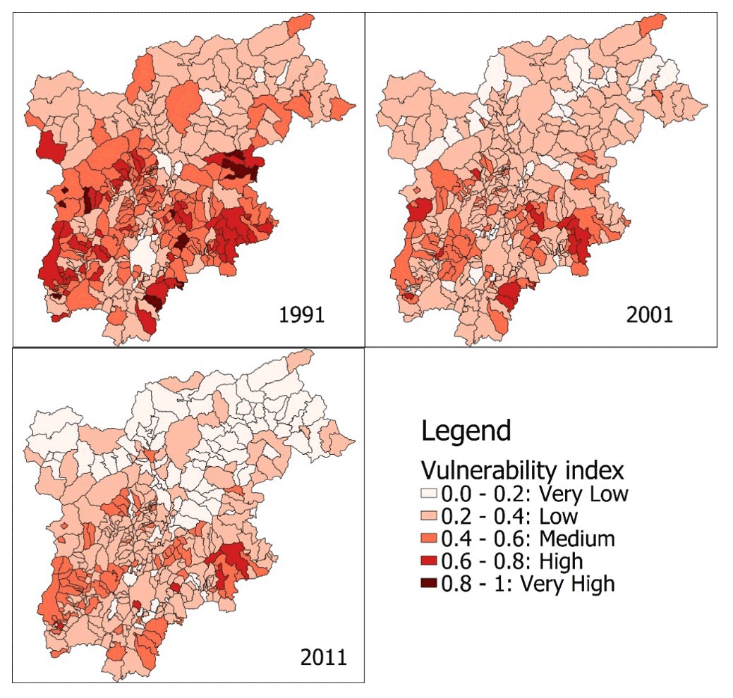
Figure 5Calculated extreme temperature vulnerability index for the 3 years of the census records (1991, 2001, 2011) with the borders of the municipalities in black.
4.4 Risk quantification
Figure 6 shows the trend in risk for the whole region over the period 1980–2018. The robust linear model shows a significant increasing trend for HW risk in 40 % of the region's area, with a significant decreasing risk in some isolated parts of the region of study. While the risk from CWs has decreased over most of the region since the 1980s, an increase is found in the major cities (Trento, Rovereto, Bolzano, and Merano).

Figure 6Trends between 1980 and 2018 of (a) heat waves and (b) cold waves risks using the robust linear method. Colors indicate an increase in the risk and grey a decrease. Significance is indicated with the hashing, the yearly change being the robust linear model coefficient.
Decadal means of the annual regional risk values confirm these trends, with the HW risk increasing from 0.119 in the 1980s to 0.133 for the 2010s, while CW risk has decreased from 0.134 in the 1980s to 0.124 in the 2010s. Decadal means of HW risk for the large cities show a stronger trend compared to the whole region. We found that the average HW risk in the main cities increased by nearly 45 % compared to the 12 % increase in the whole region. Decadal means of CW risk for the main cities increased by nearly 17 %, whereas in the whole region it decreased by 7 %.
The highest annual risk levels for both HWs and CWs coincide with the years with the highest hazard intensity (2003 for HW and 1985 for CW; see Fig. S5 in the Supplement), indicating that the hazard is potentially the main factor for risk. However, risks are of course further modulated by exposure and vulnerability. The risks are found to be the highest in the largest cities (Bolzano, Merano, Rovereto, and Trento).
Figure 7 shows the marginal effect of the driving factor behind the trends in HW and CW risks. Figure 7a, c, and e (b, d, and f) show the trend in HWs (CWs) risks with only vulnerability, only exposure, and only hazard changing, respectively.
Figure 7a and b show trends in risk due to changes in vulnerability only, effectively indicating the locations of the increases/decreases in risk due the changes of vulnerability indicators, which are equally weighted (seen in Fig. 5). These trends are found to be increasing in the main cities and nearby areas and are found to be decreasing for the rest of the region.
Figure 7c and d show trends in risk due to change in exposure only, indicating the locations of changing risk due to the changes in population (exposed) only. The HW and CW risks are found to be increasing in or near urban areas and decreasing in zones at high elevations and far from the urban centers.
Figure 7e shows the trends in HW risk due to hazard only, with statistically significant increasing trends being more evident in and around highly populated areas. The figure shows that hazard is the main driver of risk for HWs, with the significant increasing hazard trends canceling (as can be seen in Fig. 6a) most of the significant decreasing trends of the other two elements (exposure and vulnerability) seen in the Fig. 7a and c.
Finally, Fig. 7f shows no significant trends in CW risk due to change in hazards only. The figure indicates that the combination of three elements of the risk equation (Eq. 9) is the main driver of its risk (Fig. 6b) rather than the CW hazard only.
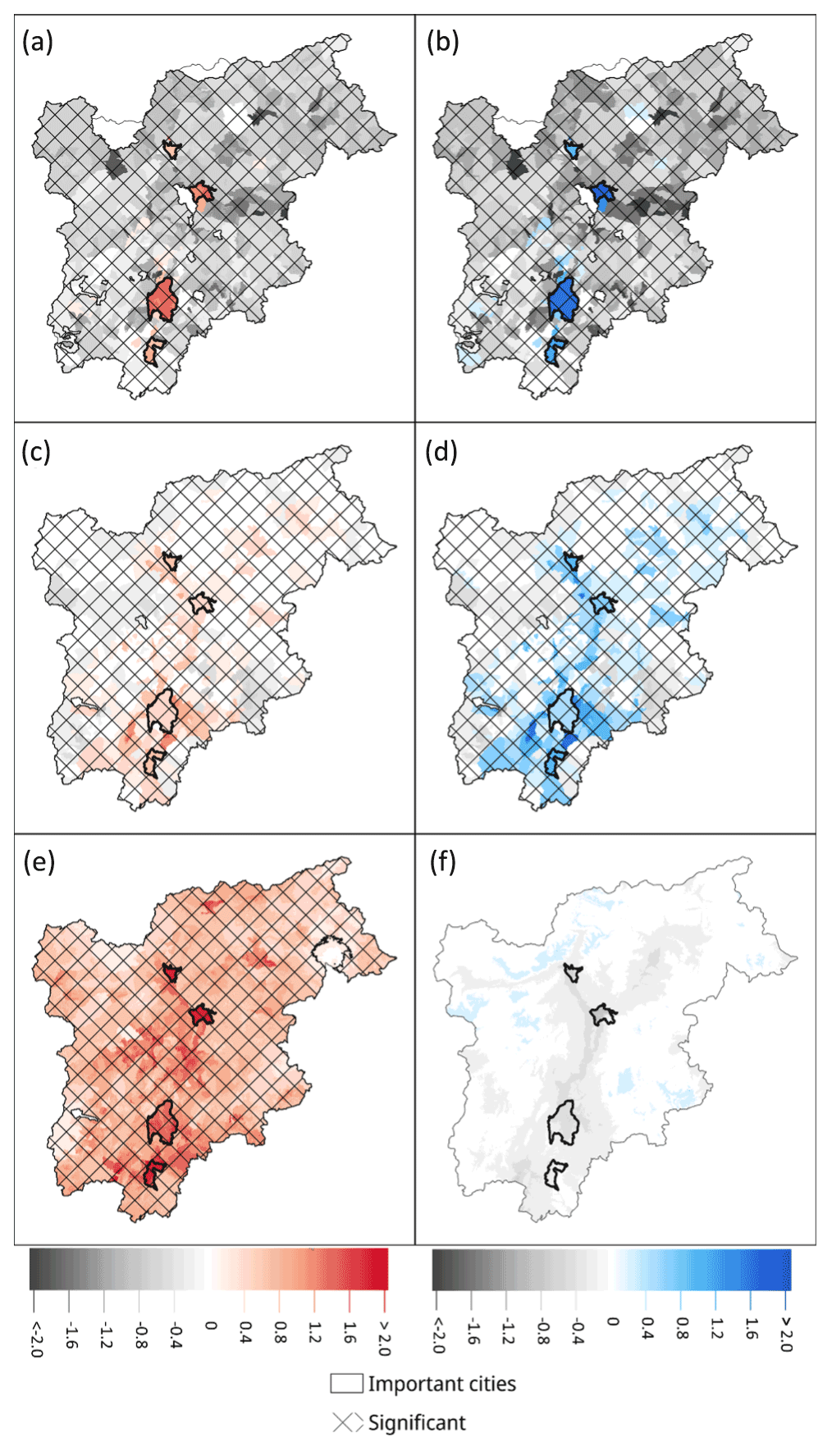
Figure 7Trends between 1980 and 2018 of heat wave risks, panel (a) (c) and (e), and cold wave risks, panel (b) (d) and (f) due to changes in vulnerability only, i.e. panel (a, b); exposure only, i.e. panel (c, d), and hazard only, i.e. panel (e, f). Trends are found with the robust linear method, with red (blue) colors indicating an increase in the risk and grey a decrease. Significance is indicated with the hashing, the yearly change (× 10−3) being the robust linear model coefficient.
The hazard analysis presented in this paper relies on the Crespi et al. (2021) air temperature database. Although the work of Crespi et al. (2021) is based on a state-of-the-art interpolation approach and represents the best product for the area, more attention should be given to measuring meteorological variables in orographically complex areas and at high elevation. A more in-depth analysis of this sort will in turn reduce uncertainty in spatial interpolation and improve the quantification of hazards such as HWs and CWs and related risks.
The findings of this study agree with Russo et al. (2015), who found the greatest HWs in the region in 1983, 2003, and 2015 in their analysis of Europe since 1950. The fact that four of the six largest HWs occurred in the last decade suggests that climate change is already influencing the intensity and frequency of HWs in the Trentino-Alto Adige region. Regarding CWs, Jarzyna and Krzyżewska (2021) also found cold spells in the years 1985 and 2012 using different methodologies for other locations throughout Europe. Similarly, other studies found 1985 to be a year of an exceptional CW in Europe (Spinoni et al., 2015; Twardosz and Kossowska-Cezak, 2016).
Figure 3a indicates that a strong increase in heat wave trends is observed in the northwest and the north of our study area. Both areas are at a high elevation (between ∼ 1000 m and ∼ 3900 m), and one includes the highest mountain in the analyzed area. These results are consistent with those presented by Acquaotta et al. (2015), who found higher increases in temperatures at higher elevations in northwestern Italy.
Our results for HWs are also in line with the finding of Bacco et al. (2020) that analyzed trends in temperature extremes over northeastern regions of Italy (including Trentino-Alto Adige) based on homogenized data from dense station networks. Bacco et al. (2021) also found widespread warming, with significant positive trends in maximum-related mean and daytime temperature extremes. The lack of trend in CW events is also in agreement with previous research that could not detect any trend in extreme cold spells (Jarzyna and Krzyżewska, 2021; Piticar et al., 2018).
The trends in vulnerability and their absence of statistical significance strongly depend on the available data. In our case the data used are from the specific national census carried out every 10 years and aggregated at the city spatial scale. These data are freely available and allow us to quantify the vulnerability to natural hazards, which is a crucial component for the risk quantification (e.g., Formetta and Feyen, 2019; Frigerio and De Amicis, 2016).
Consistently with previous studies in other European regions (e.g., López-Bueno et al., 2021; Poumadère et al., 2005), we found that the elderly population and isolation were the indicators most affecting the increase in extreme temperature vulnerability.
The results of our vulnerability analysis contrast with the findings of Frigerio and De Amicis (2016), who report increasing vulnerability for municipalities of the Bolzano province and slightly decreasing to steady vulnerability in the Trento province. The contrast between their findings and ours is related to the use of different indicators (i.e., they use employment, social-economic status, family structures, race/ethnicity, and population growth) and also a different methodology for calculating the vulnerability. The methodology used by Frigerio and De Amicis (2016) normalizes indicators across all of Italy; by contrast in this study we normalize indicators over the Trentino-Alto Adige region only, allowing us to better characterize local vulnerability.
Our findings on the increase in HW risks are consistent with Smid et al. (2019), who showed an increase of risk in both current and the future period for European capitals; the same study highlights a future decrease in CW risk for these same cities. We found that CW risk is still increasing for the main cities of our study. This is also the case for other cities in mountainous regions, such as is highlighted by López-Bueno et al. (2021) for the metropolitan area of Madrid, where the urban area was found to be more at risk from CWs compared to the rural areas in the same region.
Our analysis of the risk trends shows that hazard and vulnerability are the main driving factors of HW risk in the region of study. The changes in HW risk due to hazard also highlight the presence of an urban heat island effect in the most populated cities of the region (in Fig. 7e these are the zones of the highest increasing trends in risk). This has also been found in other studies of urban areas (e.g., Morabito et al., 2021). The changes in CW risk are explained by the demographic changes (i.e., an increasing and aging population) and by other vulnerability changes, which are increasing in/around urban areas and decreasing elsewhere.
The changes found in HW and CW risk due to changes in exposure or vulnerability only is partially explained by rural–urban migration and by an aging population. Findings of rural–urban migration and aging populations are presented in other studies such as that of Reynaud and Miccoli (2018), who demonstrated these in Italy and more specifically our study area.
Our study is one of the first to calculate risks of HWs and CWs and their trends at the community and city level for a region over a 39-year period. This is done by first quantifying the historical hazard of extreme temperature events using HWMId and CWMId indicators, at high spatial resolution (250 m) in the Trentino-Alto Adige region for the period 1980–2018. The hazard probability of occurrences is then quantified by fitting the Tweedie distribution to HWMId and CWMId values, explicitly accounting for zero values in their time series. Two types of population exposure are found using different hazard return levels (5- and 10-year return level). Vulnerability is calculated using eight different socioeconomic indicators. Combining these findings, the spatiotemporal HW and CW risk over the time period and at the city level is calculated.
Over the past 4 decades, HWs, i.e., HWMId > 0 (and extreme HWs, i.e., HWMId > HW5Y) showed increasing trends in most of the region, with 98 % (70 %) being statistically significant. This results in an increasing exposure of people to extreme heat spells. For CW, we did not find a trend in hazard frequency, and intensity and exposure to extreme cold remain constant. With regards to risk, a steady increase (∼12 %) in HW risk and a decrease (∼7 %) in CW risk are found for the entire region. However, in larger cities of the region, a much stronger rise in HW risk (∼ 45 %) and CW risk (∼ 17 %) occur. This is linked with demographic changes and the social status of city inhabitants, with an increasing and aging population living in cities and an increase in the number of one-person households.
The findings of this work show that municipalities and cities in the Trentino-Alto Adige region have experienced increasing HW risk over the time frame 1980–2018 while potentially experiencing a steady level of CW risk. Our detailed analysis shows where in the region to prioritize risk mitigation measures to reduce hazard and vulnerability. Measures to mitigate heat in cities include, for example, greening of cities (Alsaad et al., 2022; Taleghani et al., 2019), while vulnerability could be decreased by improving the social and living conditions of citizens, especially of the elderly, who are more vulnerable to HWs (Orlando et al., 2021; Poumadère et al., 2005; Vu et al., 2019), particularly in the cities of this region where their share of the population is growing. If detailed data are available for temperature, exposure, and vulnerability indicators, the methodology presented here could be applied to other regions within and outside of Italy to help steer local investments in climate change adaptation at the city level.
The code used for calculating HWMId and CWMId is free and open source; it is the extRemes package of R, which is available here: https://cran.r-project.org/web/packages/extRemes/index.html (Gilleland, 2021) and https://doi.org/10.18637/jss.v072.i08 (Gilleland and Katz, 2016). The Tweedie distribution was implemented using the Tweedie package of R: https://cran.r-project.org/web/packages/tweedie/index.html (Dunn, 2021).
All data used in this study are freely available and online. The temperature data (Crespi et al., 2021) are available at the following location: https://doi.org/10.1594/PANGAEA.924502 (Crespi et al., 2020). The population data from the GHSL are available at this location: https://data.jrc.ec.europa.eu/collection/ghsl (European Comission, 2018). The indicator data used to calculate the vulnerable are available from ISTAT: https://www.istat.it/en/ (ISTAT, 2023).
The supplement related to this article is available online at: https://doi.org/10.5194/nhess-23-2593-2023-supplement.
The author contributions were as follow: Conceptualization: MM, GF, LF; Data curation: MM, GF; Formal Analysis: MM, GF; Supervision: GF; Methodology: MM, GF, SR; Writing Original draft preparation: MM, GF; Writing review and editing: LF, SR, MM, GF.
The contact author has declared that none of the authors has any competing interests.
Publisher’s note: Copernicus Publications remains neutral with regard to jurisdictional claims in published maps and institutional affiliations.
Giuseppe Formetta acknowledges funding from the Italian Ministry of Education, University and Research (MIUR) in the framework of the Departments of Excellence Initiative 2023–2027. This study was carried out also within the PNRR research activities of the consortium iNEST (Interconnected North-Est Innovation Ecosystem) funded by the European Union Next-GenerationEU (Piano Nazionale di Ripresa e Resilienza (PNRR) – Missione 4 Componente 2, Investimento 1.5 – D.D. 1058 23/06/2022, ECS_00000043). This article reflects only the authors' views and opinions.
Giuseppe Formetta acknowledges funding from the Italian Ministry of Education, University and Research (MIUR) in the framework of the Departments of Excellence Initiative 2023–2027. This study was carried out also within the PNRR research activities of the consortium iNEST (Interconnected North-Est Innovation Ecosystem) funded by the European Union Next-GenerationEU (Piano Nazionale di Ripresa e Resilienza (PNRR) – Missione 4 Componente 2, Investimento 1.5 – D.D. 1058 23/06/2022, ECS_00000043).
This paper was edited by Vassiliki Kotroni and reviewed by Clemens Schwingshackl and one anonymous referee.
Acquaotta, F., Fratianni, S., and Garzena, D.: Temperature changes in the North-Western Italian Alps from 1961 to 2010, Theor. Appl. Climatol., 122, 619–634, https://doi.org/10.1007/s00704-014-1316-7, 2015.
Alma, Ö. G.: Comparison of Robust Regression Methods in Linear Regression, Int. J. Contemp. Math. Sciences, 6, 409–421, 2011.
Alsaad, H., Hartmann, M., Hilbel, R., and Voelker, C.: The potential of facade greening in mitigating the effects of heatwaves in Central European cities, Build. Environ., 216, 109021, https://doi.org/10.1016/j.buildenv.2022.109021, 2022.
Bacco, M. D. and Scorzini, A. R.: Recent changes in temperature extremes across the north-eastern region of Italy and their relationship with large-scale circulation, Clim. Res., 81, 167–185, https://doi.org/10.3354/cr01614, 2020.
Bonat, W. H. and Kokonendji, C. C.: Flexible Tweedie regression models for continuous data, J. Stat. Comput. Simul., 87, 2138–2152, https://doi.org/10.1080/00949655.2017.1318876, 2017.
Brossart, D. F., Parker, R. I., and Castillo, L. G.: Robust regression for single-case data analysis: How can it help?, Behav. Res. Methods, 43, 710–719, https://doi.org/10.3758/s13428-011-0079-7, 2011.
Buscail, C., Upegui, E., and Viel, J.-F.: Mapping heatwave health risk at the community level for public health action, Int. J. Health Geogr., 11, 38, https://doi.org/10.1186/1476-072X-11-38, 2012.
Buzási, A.: Comparative assessment of heatwave vulnerability factors for the districts of Budapest, Hungary, Urban Clim., 42, 101127, https://doi.org/10.1016/j.uclim.2022.101127, 2022.
Ceccherini, G., Russo, S., Ameztoy, I., Marchese, A. F., and Carmona-Moreno, C.: Heat waves in Africa 1981–2015, observations and reanalysis, Nat. Hazards Earth Syst. Sci., 17, 115–125, https://doi.org/10.5194/nhess-17-115-2017, 2017.
Chambers, J.: Global and cross-country analysis of exposure of vulnerable populations to heatwaves from 1980 to 2018, Clim. Change, 163, 539–558, https://doi.org/10.1007/s10584-020-02884-2, 2020.
Cheng, W., Li, D., Liu, Z., and Brown, R. D.: Approaches for identifying heat-vulnerable populations and locations: A systematic review, Sci. Total Environ., 799, 149417, https://doi.org/10.1016/j.scitotenv.2021.149417, 2021.
Conti, S., Meli, P., Minelli, G., Solimini, R., Toccaceli, V., Vichi, M., Beltrano, C., and Perini, L.: Epidemiologic study of mortality during the Summer 2003 heat wave in Italy, Environ. Res., 98, 390–399, https://doi.org/10.1016/j.envres.2004.10.009, 2005.
Crespi, A., Matiu, M., Bertoldi, G., Petitta, M., and Zebisch, M.: A high-resolution gridded dataset of daily temperature and precipitation records (1980–2018) for Trentino-South Tyrol (north-eastern Italian Alps), Earth Syst. Sci. Data, 13, 2801–2818, https://doi.org/10.5194/essd-13-2801-2021, 2021.
Crespi, A., Matiu, M., Bertoldi, G., Petitta, M., and Zebisch, M.: High-resolution daily series (1980–2018) and monthly climatologies (1981–2010) of mean temperature and precipitation for Trentino – South Tyrol (north-eastern Italian Alps) [dataset], PANGAEA, https://doi.org/10.1594/PANGAEA.924502 (last access: 5 July 2023), 2020.
de'Donato, F. K., Leone, M., Noce, D., Davoli, M., and Michelozzi, P.: The Impact of the February 2012 Cold Spell on Health in Italy Using Surveillance Data, PLOS ONE, 8, e61720, https://doi.org/10.1371/journal.pone.0061720, 2013.
Dong, J., Peng, J., He, X., Corcoran, J., Qiu, S., and Wang, X.: Heatwave-induced human health risk assessment in megacities based on heat stress-social vulnerability-human exposure framework, Landsc. Urban Plan., 203, 103907, https://doi.org/10.1016/j.landurbplan.2020.103907, 2020.
Dosio, A., Mentaschi, L., Fischer, E. M., and Wyser, K.: Extreme heat waves under 1.5 ∘C and 2 ∘C global warming, Environ. Res. Lett., 13, 054006, https://doi.org/10.1088/1748-9326/aab827, 2018.
Dunn, P. K.: Occurrence and quantity of precipitation can be modelled simultaneously, Int. J. Climatol., 24, 1231–1239, https://doi.org/10.1002/joc.1063, 2004.
Dunn, P. K.: Tweedie: Evaluation of Tweedie exponential family models, R package version 2.3 [code], https://cran.r-project.org/web/packages/tweedie/index.html (last access: 5 July 2023), 2021.
Dunn, P. K. and Smyth, G. K.: Series evaluation of Tweedie exponential dispersion model densities, Stat. Comput., 15, 267–280, https://doi.org/10.1007/s11222-005-4070-y, 2005.
Ellena, M., Ballester, J., Mercogliano, P., Ferracin, E., Barbato, G., Costa, G., and Ingole, V.: Social inequalities in heat-attributable mortality in the city of Turin, northwest of Italy: a time series analysis from 1982 to 2018, Environ. Health, 19, 116, https://doi.org/10.1186/s12940-020-00667-x, 2020.
El-Zein, A. and Tonmoy, F. N.: Assessment of vulnerability to climate change using a multi-criteria outranking approach with application to heat stress in Sydney, Ecol. Indic., 48, 207–217, https://doi.org/10.1016/j.ecolind.2014.08.012, 2015.
Estoque, R. C., Ooba, M., Seposo, X. T., Togawa, T., Hijioka, Y., Takahashi, K., and Nakamura, S.: Heat health risk assessment in Philippine cities using remotely sensed data and social-ecological indicators, Nat. Commun., 11, 1581, https://doi.org/10.1038/s41467-020-15218-8, 2020.
European Comission: Joint Research Centre Data Catalogue: Global Human Settlement Layer, European Commission [data set], https://data.jrc.ec.europa.eu/collection/ghsl (last access: 5 July 2023), 2018.
Filzmoser, P. and Nordhausen, K.: Robust linear regression for high-dimensional data: An overview, WIREs Comput. Stat., 13, e1524, https://doi.org/10.1002/wics.1524, 2021.
Formetta, G. and Feyen, L.: Empirical evidence of declining global vulnerability to climate-related hazards, Glob. Environ. Change, 57, 101920, https://doi.org/10.1016/j.gloenvcha.2019.05.004, 2019.
Fratianni, S. and Acquaotta, F.: The Climate of Italy, in: Landscapes and Landforms of Italy, edited by: Soldati, M. and Marchetti, M., Springer International Publishing, Cham, 29–38, https://doi.org/10.1007/978-3-319-26194-2_4, 2017.
Frigerio, I. and De Amicis, M.: Mapping social vulnerability to natural hazards in Italy: A suitable tool for risk mitigation strategies, Environ. Sci. Policy, 63, 187–196, https://doi.org/10.1016/j.envsci.2016.06.001, 2016.
García-León, D., Casanueva, A., Standardi, G., Burgstall, A., Flouris, A. D., and Nybo, L.: Current and projected regional economic impacts of heatwaves in Europe, Nat. Commun., 12, 5807, https://doi.org/10.1038/s41467-021-26050-z, 2021.
Gasparrini, A., Guo, Y., Hashizume, M., Lavigne, E., Zanobetti, A., Schwartz, J., Tobias, A., Tong, S., Rocklöv, J., Forsberg, B., Leone, M., Sario, M. D., Bell, M. L., Guo, Y.-L. L., Wu, C., Kan, H., Yi, S.-M., Coelho, M. de S. Z. S., Saldiva, P. H. N., Honda, Y., Kim, H., and Armstrong, B.: Mortality risk attributable to high and low ambient temperature: a multicountry observational study, The Lancet, 386, 369–375, https://doi.org/10.1016/S0140-6736(14)62114-0, 2015.
Gilleland, E.: extRemes: Extreme Value Analysis, 2022. R package version 2.1 [code], https://cran.r-project.org/web/packages/extRemes/index.html (last access: 5 July 2023), 2021.
Gilleland, E. and Katz, R. W.: extRemes 2.0: An Extreme Value Analysis Package in R [code], J. Stat. Softw., 72, 1–39, https://doi.org/10.18637/jss.v072.i08, 2016.
Goffard, P.-O., Jammalamadaka, S. R., and Meintanis, S.: Goodness-of-fit tests for compound distributions with applications in insurance, 2019.
Habeeb, D., Vargo, J., and Stone, B.: Rising heat wave trends in large US cities, Nat. Hazards, 76, 1651–1665, https://doi.org/10.1007/s11069-014-1563-z, 2015.
Hasan, M. M. and Dunn, P. K.: Two Tweedie distributions that are near-optimal for modelling monthly rainfall in Australia, Int. J. Climatol., 31, 1389–1397, https://doi.org/10.1002/joc.2162, 2011.
Ho, H. C., Knudby, A., Chi, G., Aminipouri, M., and Lai, D. Y.-F.: Spatiotemporal analysis of regional socio-economic vulnerability change associated with heat risks in Canada, Appl. Geogr., 95, 61–70, https://doi.org/10.1016/j.apgeog.2018.04.015, 2018.
Huber, P. J.: Robust Statistics, in: International Encyclopedia of Statistical Science, edited by: Lovric, M., Springer, Berlin, Heidelberg, 1248–1251, https://doi.org/10.1007/978-3-642-04898-2_594, 2011.
IPCC: Climate Change 2014 – Impacts, Adaptation and Vulnerability: Part A: Global and Sectoral Aspects: Working Group II Contribution to the IPCC Fifth Assessment Report: Volume 1: Global and Sectoral Aspects, Cambridge University Press, Cambridge, https://doi.org/10.1017/CBO9781107415379, 2014.
Istat.it – 15∘ Censimento della popolazione e delle abitazioni 2011: https://www.istat.it/it/censimenti-permanenti/censimenti-precedenti/popolazione-e-abitazioni/popolazione-2011, last access: 16 November 2021.
ISTAT: Webpage of the Italian National Institute of Statistics, Istat [data set], https://www.istat.it/en/ (last access: 5 July 2023), 2023.
Jarzyna, K. and Krzyżewska, A.: Cold spell variability in Europe in relation to the degree of climate continentalism in 1981–2018 period, Weather, 76, 122–128, https://doi.org/10.1002/wea.3937, 2021.
Johnson, W. D., Burton, J. H., Beyl, R. A., and Romer, J. E.: A Simple Chi-Square Statistic for Testing Homogeneity of Zero-Inflated Distributions, Open J. Stat., 5, 483, https://doi.org/10.4236/ojs.2015.56050, 2015.
Jorgensen, B.: Exponential Dispersion Models, J. R. Stat. Soc. Ser. B Methodol., 49, 127–162, 1987.
Karanja, J. and Kiage, L.: Perspectives on spatial representation of urban heat vulnerability, Sci. Total Environ., 774, 145634, https://doi.org/10.1016/j.scitotenv.2021.145634, 2021.
Khan, D. M., Yaqoob, A., Zubair, S., Khan, M. A., Ahmad, Z., and Alamri, O. A.: Applications of Robust Regression Techniques: An Econometric Approach, Math. Probl. Eng., 2021, e6525079, https://doi.org/10.1155/2021/6525079, 2021.
Kim, D.-W., Deo, R. C., Lee, J.-S., and Yeom, J.-M.: Mapping heatwave vulnerability in Korea, Nat. Hazards, 89, 35–55, https://doi.org/10.1007/s11069-017-2951-y, 2017.
King, A. D. and Harrington, L. J.: The Inequality of Climate Change From 1.5 to 2 ∘C of Global Warming, Geophys. Res. Lett., 45, 5030–5033, https://doi.org/10.1029/2018GL078430, 2018.
King, A. D., Donat, M. G., Lewis, S. C., Henley, B. J., Mitchell, D. M., Stott, P. A., Fischer, E. M., and Karoly, D. J.: Reduced heat exposure by limiting global warming to 1.5 ∘C, Nat. Clim. Change, 8, 549–551, https://doi.org/10.1038/s41558-018-0191-0, 2018.
Kishore, P., Basha, G., Venkat Ratnam, M., AghaKouchak, A., Sun, Q., Velicogna, I., and Ouarda, T. B. J. M.: Anthropogenic influence on the changing risk of heat waves over India, Sci. Rep., 12, 3337, https://doi.org/10.1038/s41598-022-07373-3, 2022.
Kron, W., Löw, P., and Kundzewicz, Z. W.: Changes in risk of extreme weather events in Europe, Environ. Sci. Policy, 100, 74–83, https://doi.org/10.1016/j.envsci.2019.06.007, 2019.
Leung, S., Thompson, L., McPhaden, M. J., and Mislan, K. A. S.: ENSO drives near-surface oxygen and vertical habitat variability in the tropical Pacific, Environ. Res. Lett., 14, 064020, https://doi.org/10.1088/1748-9326/ab1c13, 2019.
Liu, X., Yue, W., Yang, X., Hu, K., Zhang, W., and Huang, M.: Mapping Urban Heat Vulnerability of Extreme Heat in Hangzhou via Comparing Two Approaches, Complexity, 2020, e9717658, https://doi.org/10.1155/2020/9717658, 2020.
López-Bueno, J. A., Navas-Martín, M. Á., Díaz, J., Mirón, I. J., Luna, M. Y., Sánchez-Martínez, G., Culqui, D., and Linares, C.: The effect of cold waves on mortality in urban and rural areas of Madrid, Environ. Sci. Eur., 33, 72, https://doi.org/10.1186/s12302-021-00512-z, 2021.
Michelozzi, P., de 'Donato, F., Bisanti, L., Russo, A., Cadum, E., DeMaria, M., D'Ovidio, M., Costa, G., and Perucci, C. A.: Heat Waves in Italy: Cause Specific Mortality and the Role of Educational Level and Socio-Economic Conditions, in: Extreme Weather Events and Public Health Responses, edited by: Kirch, W., Bertollini, R., and Menne, B., Springer, Berlin, Heidelberg, 121–127, https://doi.org/10.1007/3-540-28862-7_12, 2005.
Michelozzi, P., De' Donato, F., Scortichini, M., De Sario, M., Asta, F., Agabiti, N., Guerra, R., de Martino, A., and Davoli, M.: [On the increase in mortality in Italy in 2015: analysis of seasonal mortality in the 32 municipalities included in the Surveillance system of daily mortality], Epidemiol. Prev., 40, 22–28, https://doi.org/10.19191/EP16.1.P022.010, 2016.
Morabito, M., Crisci, A., Gioli, B., Gualtieri, G., Toscano, P., Stefano, V. D., Orlandini, S., and Gensini, G. F.: Urban-Hazard Risk Analysis: Mapping of Heat-Related Risks in the Elderly in Major Italian Cities, PLOS ONE, 10, e0127277, https://doi.org/10.1371/journal.pone.0127277, 2015.
Morabito, M., Crisci, A., Guerri, G., Messeri, A., Congedo, L., and Munafò, M.: Surface urban heat islands in Italian metropolitan cities: Tree cover and impervious surface influences, Sci. Total Environ., 751, 142334, https://doi.org/10.1016/j.scitotenv.2020.142334, 2021.
Neumayer, E. and Barthel, F.: Normalizing economic loss from natural disasters: A global analysis, Glob. Environ. Change, 21, 13–24, https://doi.org/10.1016/j.gloenvcha.2010.10.004, 2011.
Orlando, S., Mosconi, C., De Santo, C., Emberti Gialloreti, L., Inzerilli, M. C., Madaro, O., Mancinelli, S., Ciccacci, F., Marazzi, M. C., Palombi, L., and Liotta, G.: The Effectiveness of Intervening on Social Isolation to Reduce Mortality during Heat Waves in Aged Population: A Retrospective Ecological Study, Int. J. Environ. Res. Public. Health, 18, 11587, https://doi.org/10.3390/ijerph182111587, 2021.
Papathoma-Köhle, M., Ulbrich, T., Keiler, M., Pedoth, L., Totschnig, R., Glade, T., Schneiderbauer, S., and Eidswig, U.: Chapter 8 - Vulnerability to Heat Waves, Floods, and Landslides in Mountainous Terrain: Test Cases in South Tyrol, in: Assessment of Vulnerability to Natural Hazards, edited by: Birkmann, J., Kienberger, S., and Alexander, D. E., Elsevier, 179–201, https://doi.org/10.1016/B978-0-12-410528-7.00008-4, 2014.
Peng, J., Liu, Y., Li, T., and Wu, J.: Regional ecosystem health response to rural land use change: A case study in Lijiang City, China, Ecol. Indic., 72, 399–410, https://doi.org/10.1016/j.ecolind.2016.08.024, 2017.
Perkins-Kirkpatrick, S. E. and Gibson, P. B.: Changes in regional heatwave characteristics as a function of increasing global temperature, Sci. Rep., 7, 12256, https://doi.org/10.1038/s41598-017-12520-2, 2017.
Piticar, A., Croitoru, A.-E., Ciupertea, F.-A., and Harpa, G.-V.: Recent changes in heat waves and cold waves detected based on excess heat factor and excess cold factor in Romania, Int. J. Climatol., 38, 1777–1793, https://doi.org/10.1002/joc.5295, 2018.
Poumadère, M., Mays, C., Le Mer, S., and Blong, R.: The 2003 Heat Wave in France: Dangerous Climate Change Here and Now, Risk Anal., 25, 1483–1494, https://doi.org/10.1111/j.1539-6924.2005.00694.x, 2005.
Quader, M. A., Khan, A. U., and Kervyn, M.: Assessing Risks from Cyclones for Human Lives and Livelihoods in the Coastal Region of Bangladesh, Int. J. Environ. Res. Public. Health, 14, E831, https://doi.org/10.3390/ijerph14080831, 2017.
Rahma, A. and Kokonendji, C. C.: Discriminating between and within (semi)continuous classes of both Tweedie and geometric Tweedie models, J. Stat. Comput. Simul., 92, 794–812, https://doi.org/10.1080/00949655.2021.1975281, 2022.
Reid, C. E., O'Neill, M. S., Gronlund, C. J., Brines, S. J., Brown, D. G., Diez-Roux, A. V., and Schwartz, J.: Mapping Community Determinants of Heat Vulnerability, Environ. Health Perspect., 117, 1730–1736, https://doi.org/10.1289/ehp.0900683, 2009.
Reynaud, C. and Miccoli, S.: Depopulation and the Aging Population: The Relationship in Italian Municipalities, Sustainability, 10, 1004, https://doi.org/10.3390/su10041004, 2018.
Russo, S., Sillmann, J., and Fischer, E. M.: Top ten European heatwaves since 1950 and their occurrence in the coming decades, Environ. Res. Lett., 10, 124003, https://doi.org/10.1088/1748-9326/10/12/124003, 2015.
Russo, S., Marchese, A. F., Sillmann, J., and Immé, G.: When will unusual heat waves become normal in a warming Africa?, Environ. Res. Lett., 11, 054016, https://doi.org/10.1088/1748-9326/11/5/054016, 2016.
Russo, S., Sillmann, J., Sippel, S., Barcikowska, M. J., Ghisetti, C., Smid, M., and O'Neill, B.: Half a degree and rapid socioeconomic development matter for heatwave risk, Nat. Commun., 10, 136, https://doi.org/10.1038/s41467-018-08070-4, 2019.
Schiavina, M., Freire, S., and MacManus, K.: GHS-POP R2019A – GHS population grid multitemporal (1975-1990-2000-2015), https://doi.org/10.2905/0C6B9751-A71F-4062-830B-43C9F432370F, 2019.
Shono, H.: Application of the Tweedie distribution to zero-catch data in CPUE analysis, Fish. Res., 93, 154–162, https://doi.org/10.1016/j.fishres.2008.03.006, 2008.
Smid, M., Russo, S., Costa, A. C., Granell, C., and Pebesma, E.: Ranking European capitals by exposure to heat waves and cold waves, Urban Clim., 27, 388–402, https://doi.org/10.1016/j.uclim.2018.12.010, 2019.
Spinoni, J., Lakatos, M., Szentimrey, T., Bihari, Z., Szalai, S., Vogt, J., and Antofie, T.: Heat and cold waves trends in the Carpathian Region from 1961 to 2010, Int. J. Climatol., 35, 4197–4209, https://doi.org/10.1002/joc.4279, 2015.
Taleghani, M., Marshall, A., Fitton, R., and Swan, W.: Renaturing a microclimate: The impact of greening a neighbourhood on indoor thermal comfort during a heatwave in Manchester, UK, Sol. Energy, 182, 245–255, https://doi.org/10.1016/j.solener.2019.02.062, 2019.
Temple, S. D.: The Tweedie Index Parameter and Its Estimator An Introduction with Applications to Actuarial Ratemaking, BSc. Thesis, Department of Mathemeatics, University of Oregon, USA, 87 pp., 2018.
Tijdeman, E., Stahl, K., and Tallaksen, L. M.: Drought Characteristics Derived Based on the Standardized Streamflow Index: A Large Sample Comparison for Parametric and Nonparametric Methods, Water Resour. Res., 56, e2019WR026315, https://doi.org/10.1029/2019WR026315, 2020.
Tuholske, C., Caylor, K., Funk, C., Verdin, A., Sweeney, S., Grace, K., Peterson, P., and Evans, T.: Global urban population exposure to extreme heat, P. Natl. Acad. Sci. USA, 118, e2024792118, https://doi.org/10.1073/pnas.2024792118, 2021.
Twardosz, R. and Kossowska-Cezak, U.: Exceptionally cold and mild winters in Europe (1951–2010), Theor. Appl. Climatol., 125, 399–411, https://doi.org/10.1007/s00704-015-1524-9, 2016.
Tweedie, M. C. K.: An index which distinguishes between some important exponential families, in: Statistics: applications and new directions (Calcutta, 1981), Indian Statist. Inst., Calcutta, 579–604, 1984.
UNDRR, Disaster risk: https://www.undrr.org/terminology/disaster-risk, last access: 21 November 2021.
van Oldenborgh, G. J., Mitchell-Larson, E., Vecchi, G. A., Vries, H. de, Vautard, R., and Otto, F.: Cold waves are getting milder in the northern midlatitudes, Environ. Res. Lett., 14, 114004, https://doi.org/10.1088/1748-9326/ab4867, 2019.
Vu, A., Rutherford, S., and Phung, D.: Heat Health Prevention Measures and Adaptation in Older Populations – A Systematic Review, Int. J. Environ. Res. Public. Health, 16, 4370, https://doi.org/10.3390/ijerph16224370, 2019.
Watts, N., Amann, M., Arnell, N., Ayeb-Karlsson, S., Belesova, K., Berry, H., Bouley, T., Boykoff, M., Byass, P., Cai, W., Campbell-Lendrum, D., Chambers, J., Daly, M., Dasandi, N., Davies, M., Depoux, A., Dominguez-Salas, P., Drummond, P., Ebi, K. L., Ekins, P., Montoya, L. F., Fischer, H., Georgeson, L., Grace, D., Graham, H., Hamilton, I., Hartinger, S., Hess, J., Kelman, I., Kiesewetter, G., Kjellstrom, T., Kniveton, D., Lemke, B., Liang, L., Lott, M., Lowe, R., Sewe, M. O., Martinez-Urtaza, J., Maslin, M., McAllister, L., Mikhaylov, S. J., Milner, J., Moradi-Lakeh, M., Morrissey, K., Murray, K., Nilsson, M., Neville, T., Oreszczyn, T., Owfi, F., Pearman, O., Pencheon, D., Pye, S., Rabbaniha, M., Robinson, E., Rocklöv, J., Saxer, O., Schütte, S., Semenza, J. C., Shumake-Guillemot, J., Steinbach, R., Tabatabaei, M., Tomei, J., Trinanes, J., Wheeler, N., Wilkinson, P., Gong, P., Montgomery, H., and Costello, A.: The 2018 report of the Lancet Countdown on health and climate change: shaping the health of nations for centuries to come, The Lancet, 392, 2479–2514, https://doi.org/10.1016/S0140-6736(18)32594-7, 2018.
Wilks, D. S.: “The Stippling Shows Statistically Significant Grid Points”: How Research Results are Routinely Overstated and Overinterpreted, and What to Do about It, B. Am. Meteorol. Soc., 97, 2263–2273, https://doi.org/10.1175/BAMS-D-15-00267.1, 2016.