the Creative Commons Attribution 4.0 License.
the Creative Commons Attribution 4.0 License.
 | 22 Mar 2022
Ground motion prediction maps using seismic-microzonation data and machine learning
Amerigo Mendicelli
Gaetano Falcone
Gianluca Acunzo
Rose Line Spacagna
Giuseppe Naso
Massimiliano Moscatelli
Past seismic events worldwide demonstrated that damage and death toll depend on both the strong ground motion (i.e., source effects) and the local site effects. The variability of earthquake ground motion distribution is caused by the local stratigraphic and/or topographic setting and buried morphologies (e.g., irregular sub-interface between soft and stiff soils) that can give rise to amplification and resonances with respect to the ground motion expected at the reference site. Therefore, local site conditions can affect an area with damage related to the full collapse or loss in functionality of facilities, roads, pipelines, and other lifelines. To this concern, the near-real-time prediction of ground motion variation over large areas is a crucial issue to support the rescue and operational interventions. A machine learning approach was adopted to produce ground motion prediction maps considering both stratigraphic and morphological conditions. A set of about 16 000 accelerometric data points and about 46 000 geological and geophysical data points was retrieved from Italian and European databases. The intensity measures of interest were estimated based on nine input proxies. The adopted machine learning regression model (i.e., Gaussian process regression) allows for improving both the precision and the accuracy in the estimation of the intensity measures with respect to the available near-real-time prediction methods (i.e., ground motion prediction equation and ShakeMaps). In addition, maps with a 50 m × 50 m resolution were generated, providing a ground motion variability in agreement with the results of advanced numerical simulations based on detailed subsoil models.
- Article
(28143 KB) - Full-text XML
-
Supplement
(3800 KB) - BibTeX
- EndNote


Spatial distributions of ground motion induced by seismic events should be properly estimated to support risk mitigation policies over large areas. Moreover, seismic-risk analysis, extended to spatially distributed anthropic systems, presents new challenges in characterizing the seismic-risk input, regarding the spatial correlation of the ground motion values where the spatial correlation is the spatial characteristics of the ground motion arising from similarities in the seismic-wave paths and local site effects. The ShakeMaps (Wald et al., 2021), provided by the US Geological Survey, are used globally for post-earthquake emergency management and response, engineering analyses, financial instruments, and other decision-making activities. Moreover, in Italy post-event ShakeMaps are delivered by the National Institute of Geophysics and Volcanology (Michelini et al., 2019; ShakeMap, 2021). Such ShakeMaps are based on ground motion prediction equation (GMPE; among others Bindi et al., 2011) and data recorded from accelerometric stations when available.
Recently, artificial-intelligence-based procedures were proposed to produce near-real-time ground motion in terms of acceleration time histories (Jozinović et al., 2021; Tamhidi et al., 2021) and intensity measure (briefly, IM; among others Kubo et al., 2020). In general, ground motion maps were generated using earthquake source parameters (location, magnitude, and the finite fault if available); IM (peak ground acceleration, peak ground velocity, and spectral acceleration, briefly named PGA, PGV, and Sa, respectively) at the recording accelerometric stations; and the mean shear-wave velocity in the upper 30 m, VS30, as a proxy to account for site lithostratigraphic amplifications. Having ShakeMaps only when the first location and magnitude estimation are available, Jozinović et al. (2021) propose to use waveforms to predict the ground motion intensity by means of a machine learning (briefly, ML) approach (i.e., it utilizes only a training set of earthquake waveforms recorded at a pre-configured network of recording stations). Moreover, ML has been adopted to produce seismic-amplification factors maps, as in the Japan case study proposed by Kim et al. (2020), rather than to provide ground motion maps. Finally, Zhou et al. (2020) propose a seismic topographic-effect prediction model.
Overall, the abovementioned works have pointed out the following.
-
Hypocentral depth (H), epicentral distance (R), and magnitude (M) are widely used to estimate ground motion over large areas considering the source effect. Moreover, H, R, and M are provided a few minutes after an earthquake.
-
VS30, the fundamental frequency of the deposit (f0), and the depth to the engineering bedrock (H800) are the key parameters which gauge well the effect of local subsoil conditions on the seismic-wave propagation (i.e., lithostratigraphic effect). The only VS30 was used in the adopted ML approach, since the Italian VS30 map was provided by Mori et al. (2020a), while national f0 and H800 maps are not currently available.
-
Elevation (h), topographic gradients (hx and hy, where x and y are two orthogonal directions), and second-order topographic gradients (hxx and hyy) are proxies which allow for describing the morphological effects on the seismic-amplification phenomena.
In this view, this work focuses on the improvement of ground motion prediction over large areas by using the ML technique. The main task of this work is to suggest a procedure including all the main key parameters together (i.e., H, R, M, VS30, h, hx, hy, hxx, and hyy).
The damage pattern induced by seismic events is related to both geological/geomorphological conditions and the vulnerability of structures and infrastructures (Brando et al., 2020; Fayjaloun et al., 2021; Mori et al., 2020b, 2019). The ground motion prediction (i.e., seismic site response) is generally evaluated by means of numerical simulations which are time consuming and require well-detailed models capable of properly representing subsoil and topographic conditions (see, for example, Bouckovalas and Papadimitriou, 2005; Falcone et al., 2020a, b, 2018; Gatmiri and Arson, 2008; Gazetas, 1982; Luo et al., 2020; Moscatelli et al., 2020b; Pagliaroli et al., 2014; Pitilakis et al., 1999; Régnier et al., 2016, 2018).
Hence, the ML approach was adopted to
- i
implement the H, R, and M parameters available a few minutes after a seismic event;
- ii
include both lithostratigraphic (VS30) and morphological effects (h, hx, hy, hxx, and hyy);
- iii
capture the spatial correlation at short distances (hundreds of meters) due to local site effects, which is essential for reliable hazard assessments.
The main results of these elaborations are ground motion prediction maps (i.e., PGA, PGV, and Sa) with the resolution of 50 m × 50 m, which can reproduce the variability captured by advanced numerical modeling.
Seismological data (i.e., H, R, M, PGA, PGV, and Sa) retrieved from European and Italian networks (Luzi et al., 2016, 2019, 2020); geological, geophysical, and geotechnical data from seismic-microzonation (hereafter SM) studies (DPC, 2021); and morphological data (ALOS, 2021) are presented in Sect. 2. The ML approach is discussed in Sect. 3. In detail, the Sect. 3.1 is focused on the adopted ML approach in terms of training and validation phase. Performances, presented in terms of root mean square error (RMSE) and residuals (i.e., difference between the base-10 logarithms of observed and predicted values of PGA, PGV, and Sa), are compared to the results proposed by other studies (Jozinović et al., 2021; Michelini et al., 2019; Bindi et al., 2011).
For the seismic sequence that hit central Italy in 2016–2017, ML results and maps are shown in Sects. 3.2 and 4, respectively. Referring to the seismic event that occurred in central Italy on 30 October 2016, a test is proposed in Sect. 3.2 in terms of residuals of the ground motion IMs (i.e., PGA, PGV, and Sa). Ground motion prediction maps for the central Italy event that occurred on 24 August 2016 (i.e., the first destructive event of the central Italy seismic sequence for which a large number of studies have been published) are shown in Sect. 4 to demonstrate the capability of the proposed ML approach to gauge the ground motion variability at the urban scale. Moreover, with reference to Sect. 4, the ground motion profiles, based on the proposed ML approach, are compared with results obtained by means of two completely different methodologies: 2D numerical modeling of seismic site response (Gaudiosi et al., 2021; Giallini et al., 2020; Grelle et al., 2020) and the mean values predicted by the Italian ShakeMap (2021).
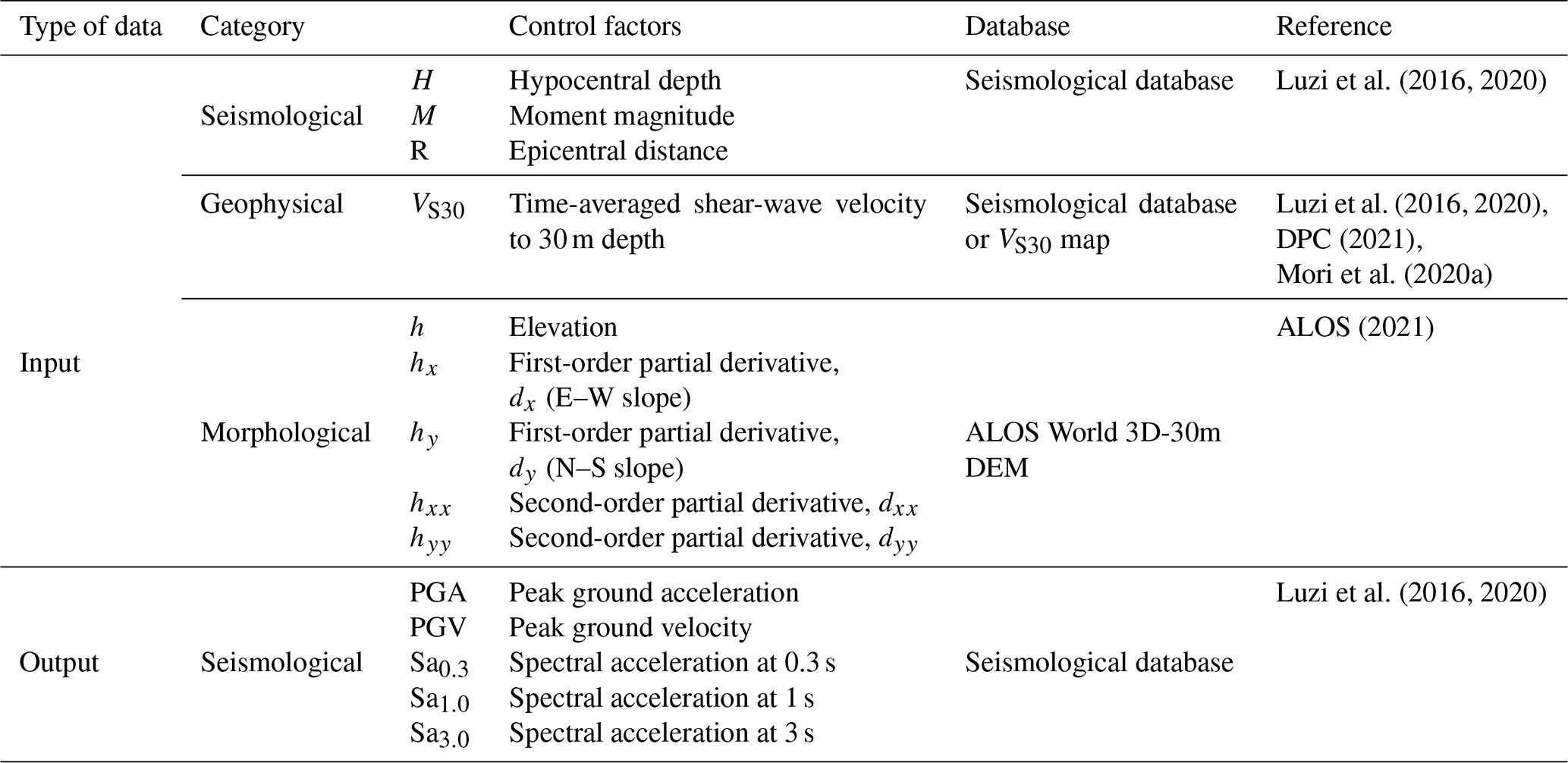
The input and output data for the training of the ML approach were classified into three categories: seismological, geophysical, and morphological data. The ML approach was based on 15 779 seismological data points regarding the log10 geometric mean of the horizontal component (geoH) for each IM (i.e., PGA, PGV, and Sa at 0.3, 1.0, and 3.0 s). Each value recorded by the accelerometric station, named output data in Table 1 (i.e., data to be reproduced by means of ML), represents an observed datum. In addition, Table 1 lists the nine used predictors, named input data. Figure 1 shows the location of the selected accelerometric stations. Figures 2 and 3 show the input and output data, respectively, adopted for the training phase of the selected ML approach and presented in this section. Furthermore, some data distributions seem to be imbalanced (e.g., magnitude, M, and elevation, h; Fig. 2). An imbalanced training input dataset is characterized by an unequal distribution of values. For instance, focusing on Fig. 2 and the M distribution, the first and third quartiles are 4.1 and 5.1, respectively. Moreover, focusing on elevation distribution, the first and third quartiles are 136 and 761 m, respectively. Consequently, when the ML algorithm learns the imbalanced data (see, for example, Kubo et al., 2020), the learning focus is mainly on the fit of ground motion with a magnitude lower than 6 or on the fit of the site characterized by elevation lower than 1200 m. The imbalance of the selected training input dataset seems to be caused by a sampling bias, since no high-magnitude ground motions were registered by the available accelerometric stations and since few accelerometric stations have been installed at high elevation, where the exposition at a seismic event is very low. Hence, the training dataset cannot actually be improved. In addition, distributions of topographic gradients and VS30 are characterized by few data points with respect to steep slopes and high VS30 values. How to handle the imbalanced dataset in the regression problem was out of the scope of this work. Consequently, referring to a range of an input datum, it is expected that the lower the number of training data is, the higher the uncertainty is. To this end, referring to the output data, maps of the standard deviation are reported in Sect. 4.
Seismological parameters are retrieved from Italian and European databases. Regarding 1435 recording accelerometric stations, PGA, PGV, spectral accelerations (i.e., Sa at 0.3, 1, and 3 s), H, R, and M were retrieved from the Engineering Strong-Motion Database, briefly ESM (Luzi et al., 2016; ESM, 2021), and ITalian ACcelerometric Archive, herein ITACA (Luzi et al., 2019). In detail, data regarding the central Italy earthquake occurred in 2016 and recorded by a temporary network named 3A have been archived only in the ITACA database (ITACA, 2021). It is worth noting that Greek and Turkish seismic-event data were collected to consider an earthquake characterized by an M value greater than 6.5 and up to 7.6. Moreover, an earthquake characterized by H, R, and a log10 PGA value greater than 30, 400 km, and 2 cm s−2, respectively, were selected. It should be noted that the ITACA and ESM selected data consider the shallow active crustal region (i.e., SACR zone characterized by shallow events, H<35 km, in agreement with Michelini et al., 2019). The distributions of seismological data of the chosen events are shown in Figs. 2 and 3. The same figures also show the distribution of data described in the next part of this section.
The dynamic site condition was described by means of the time-averaged shear-wave velocity (VS) to a depth of 30 m, the VS30 parameter. It is worth noting that the VS30 parameter has been successfully adopted to gauge lithostratigraphic effect on seismic-wave propagation by Falcone et al. (2021). VS30 data (i.e., input data in the ML approach), determined by means of in situ investigations, are also archived in the ESM and ITACA databases. VS30 values were retrieved from Mori et al. (2020a) for ESM and ITACA sites not characterized by in situ surveys. Figure 2 shows the distribution of the VS30 data.
The VS30 map proposed by Mori et al. (2020a), based on SM studies, was adopted here. The SM studies have been carried out for the Italian municipalities through the funds allocated after the 2009 L'Aquila earthquake, in the framework of the Italian program for seismic-risk prevention and mitigation (Moscatelli et al., 2020a). Approximately 4000 SM studies have been already planned, representing about 99.8 % of the municipalities eligible for funding (i.e., having a 475-year return period PGA ≥ 0.125 g). Out of the 4000 planned SM studies, about 75 % have been completed and approved (DPC, 2021). The SM studies permitted the collection, classification, and archival of geological, geophysical, and geotechnical data with a uniform approach following national standard criteria (SM Working Group, 2008; TCSM, 2018). The data from in situ tests are organized into a database and georeferenced through an appropriate geographic information system (DPC, 2021). About 35 000 borehole logs and 11 300 VS profiles, related to about 1700 down-hole and 9600 MASW (multichannel analysis of surface waves) tests, were extracted from the SM dataset. Starting from the 11 300 VS profiles, VS30 values were calculated. Mori et al. (2020b) derive a large-scale VS30 map for Italy, starting from the global morphological classes after Iwahashi et al. (2018), by integrating the large amount of data from the Italian SM dataset. The VS30 map by Mori et al. (2020a) was used here to integrate data where site-specific information was not available.
The morphological elevation, h (i.e., an input morphological datum), was retrieved by the Advanced Land Observing Satellite (ALOS) World 3D-30m (herein AW3D30) digital elevation model (DEM). The free version of the DEM (ALOS, 2021) adopted here has 1 arcsec resolution, which is equivalent to approximately 30 m at the Equator. AW3D30 global DEM data were produced using the data acquired by the Panchromatic Remote-sensing Instrument for Stereo Mapping operated on the ALOS from 2006 to 2011. The Japan Aerospace Exploration Agency, which is the operator of the satellite, produced the global DEM using approximately 3 million images. Considering that the AW3D30 model is the digital surface model which represents the canopy top and building roofs' elevations, Caglar et al. (2018) found that AW3D30 is the most accurate DEM among other similar data elevation products freely available. In detail, it was shown that the AW3D30 root mean square error is equal to 1.78 m.
Finally, the GRASS GIS (Geographic Resources Analysis Support System geographic information system) command r.slope.aspect (https://grass.osgeo.org, last access: 1 September 2021) was used to generate
the other morphological proxies (i.e., hx, hy, hxx, and
hyy). Such a command generates raster maps of first- and second-order
partial derivatives from a raster map of true elevation values (i.e., AW3D30
data in this study). Figure 2 shows the distribution of the selected
morphological data.
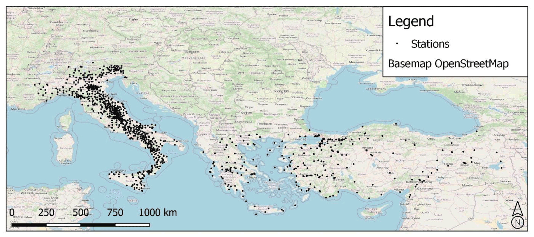
Figure 1Location of selected dataset (i.e., 1435 accelerometric stations). © OpenStreetMap. Distributed under the Open Data Commons Open Database License (ODbL) v1.0.
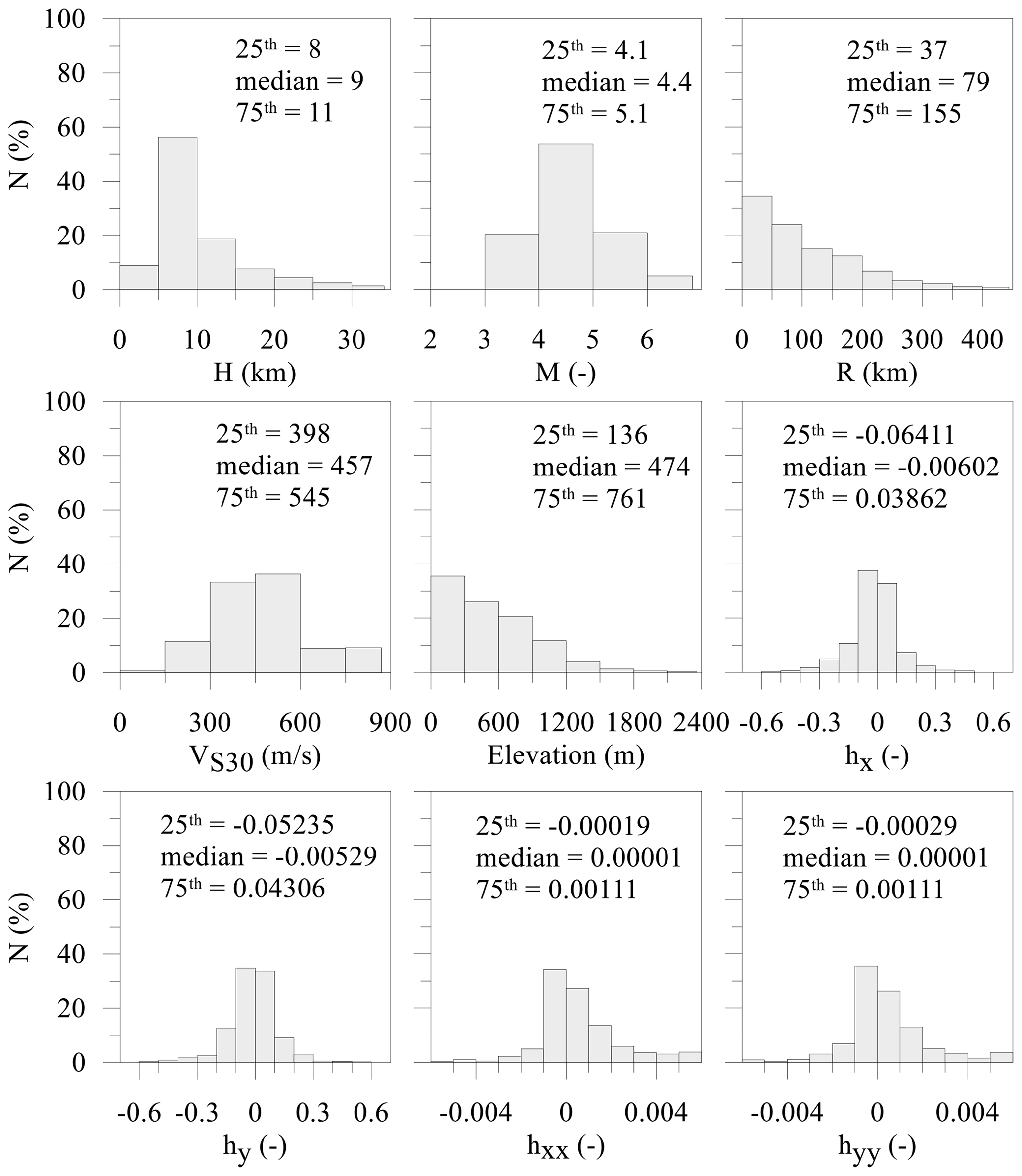
Figure 2Distribution of input data for the training dataset. N (%): counts (as a percentage).

The “MATLAB Regression Learner App” tool (https://it.mathworks.com/help/stats/regression-learner-app.html, last access: 1 September 2021) was employed to produce ground motion prediction maps using a supervised ML approach. With this application, users can choose the desired models among many different methods to automatically train and validate regression models. After training multiple models, they can be compared to choose the best one. The application includes commonly used regression methods such as linear regression models, decision trees, support vector machines, ensembles of tree models, and a Gaussian process regression (GPR).
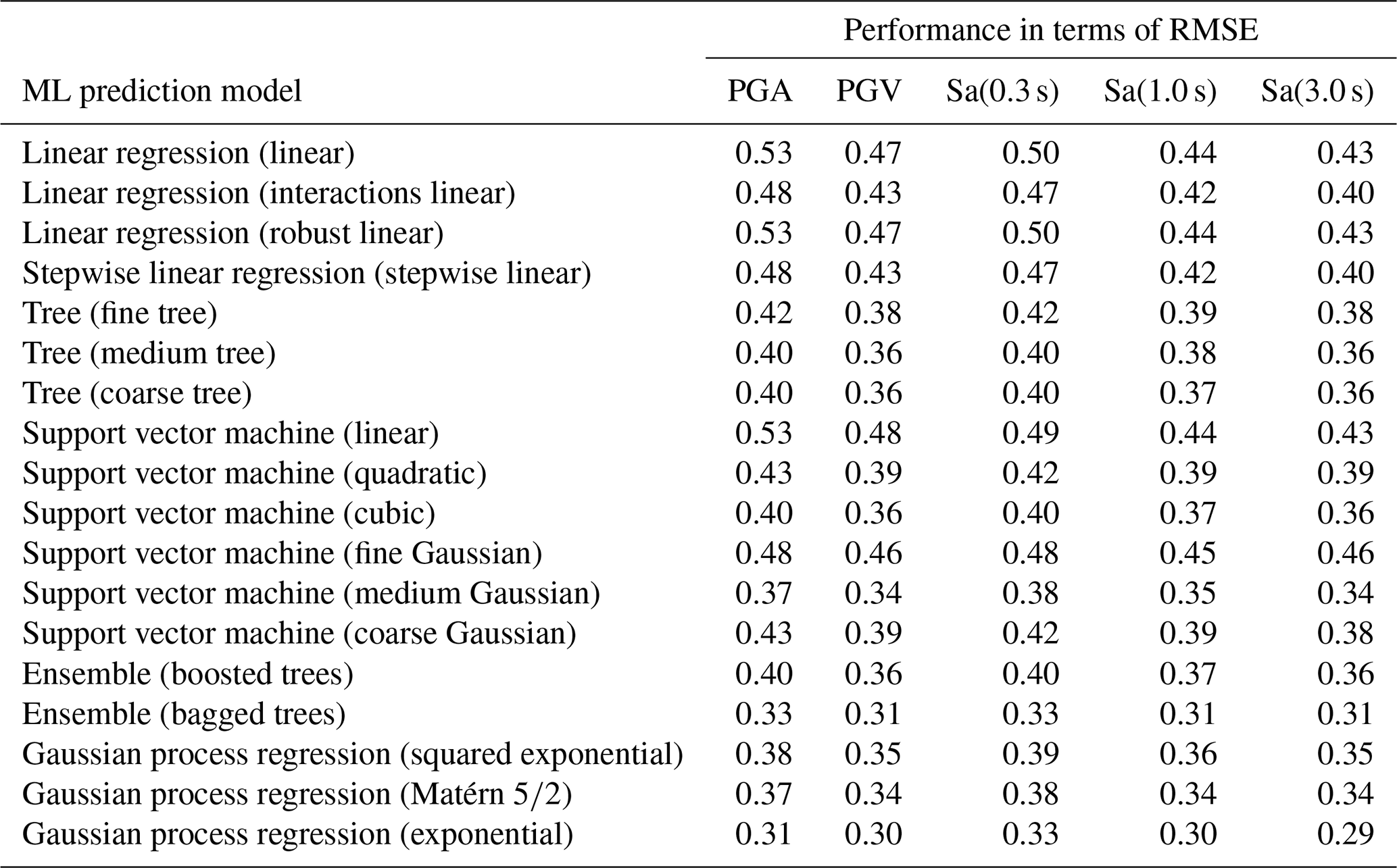
Figure 4 shows the adopted ML workflow. After having imported and selected the data (input variables and output variables), the training and validation phases begin. In these phases the ML model that will be used is “adapted”, or rather the algorithm is adapted to the training dataset. One of the objectives of this phase is the tuning of the model, acting on the hyperparameters (parameters whose value is used to control the learning process) of the algorithm to minimize errors. The k-fold cross-validation technique was used in this work. The models included in MATLAB Regression Learner App tool have all been tested. The fitting performance (in terms of RMSE) on the validation set was considered an indicator of the generalization ability of models. Among the available models the best-fitting performance in terms of RMSE was provided by the GPR model with an exponential kernel (Table 2). GPR is a nonparametric, Bayesian approach to regression, which provides uncertainty measurements on the predictions. Moreover, a detailed description of the GPR method is outside the scope of this work. Suggested references for comprehensive descriptions of the GPR method are Rasmussen and Williams (2006) and chapter 6 of MathWorks (2019). The abovementioned k-fold cross-validation (k=5) method is described in chapter 24 of MathWorks (2019).
The second step is to test the model with the best performance (GPR with an exponential kernel in this research), adopting a dataset not included in the training and validation phases. The dataset for the 30 October 2016 seismic event was used, since the accelerometric data of many accelerometric stations are available. The test is used to evaluate the accuracy of the model in terms of residuals (Eq. 1). In the workflow of Fig. 4 there is also a phase (comparison) that is not part of the standard ML methodology. The comparison with the ground shaking obtained by completely different methodologies was used to further analyze the ML model in terms of ground motion resolution and variability.
Training and cross-validation phases are described in Sect. 3.1. Comparison in terms of residuals with the performance of the existing methods (i.e., an external test) is presented in Sect. 3.2. The comparison with the ground shaking obtained by completely different methodologies is presented in Sect. 4.
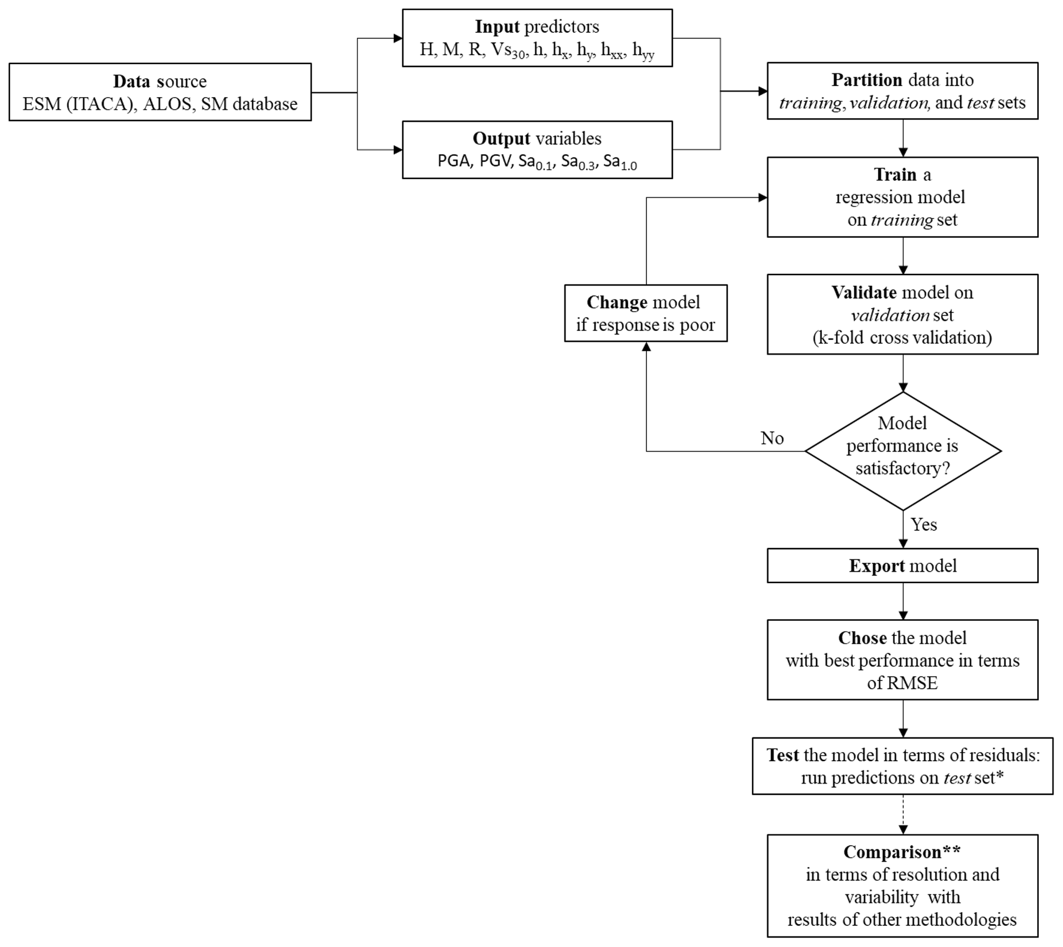
Figure 4ML workflow adopted in this study. * The selected test set was the input and output data for the 30 October 2016 seismic event. This element of the workflow is not part of the standard ML methodology. This element was introduced to enlighten the capability of the adopted ML procedure in estimating local-scale ground motion variability. Comparison against predictions from ShakeMap and 2D numerical simulations was based on 24 August 2016 seismic-event input and output data.
3.1 Training and validation phases
The mean RMSE values of the five cross-validation datasets were adopted to select the best ML approach. With reference to the tested ML approaches, Table 2 lists the RMSE values for each predicted IM.
Table 2RMSE for all ML prediction models used to forecast the log 10 geometric horizontal mean (geoH) of PGA, PGV, and Sa at 0.3, 1.0, and 3.0 s. The suggested reference for comprehensive descriptions of the ML prediction models is MathWorks (2019).
Referring to the best prediction model (i.e., GPR with an exponential kernel) and to the training dataset, Fig. 5 shows the comparison between predicted and observed values.
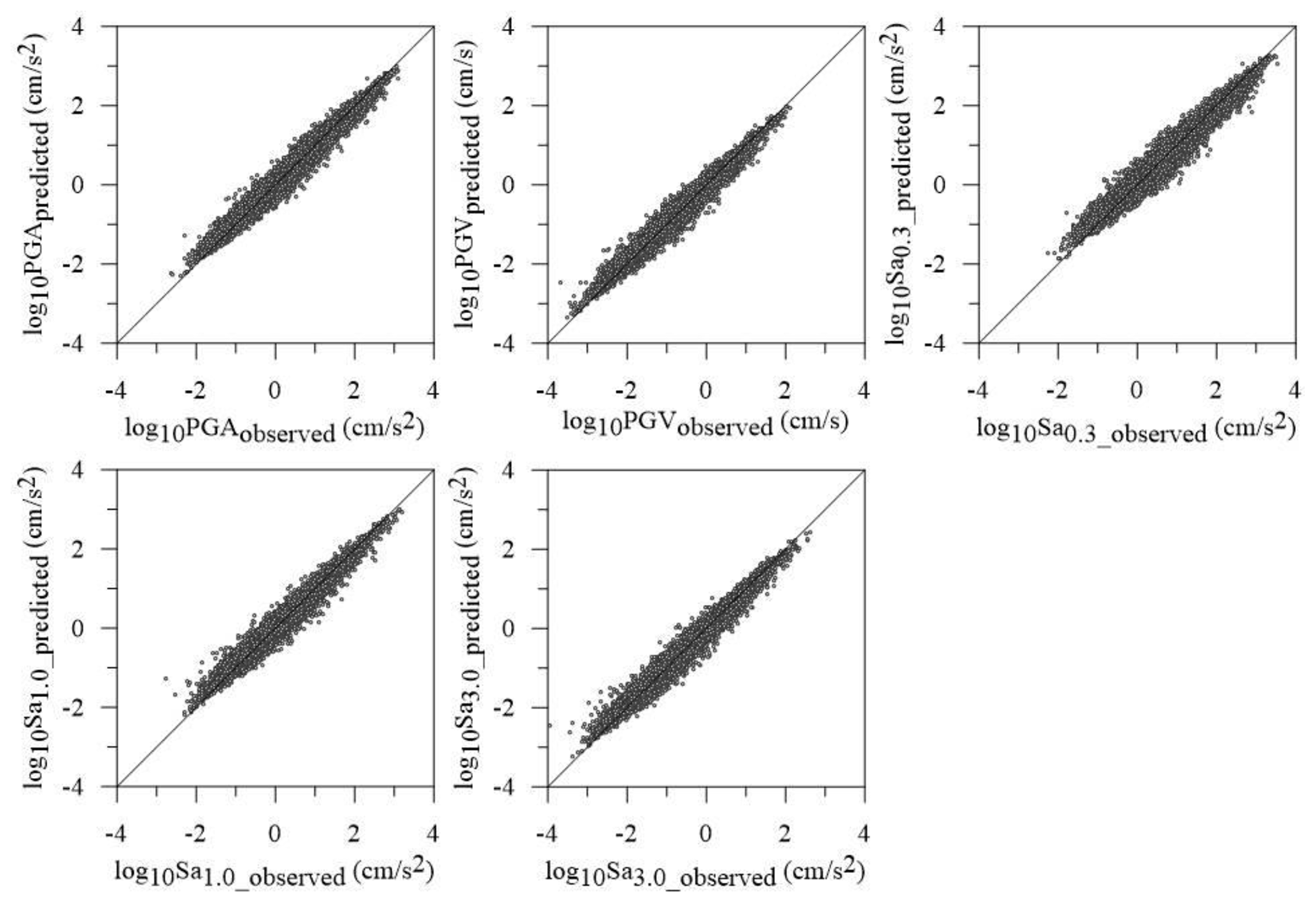
Figure 5Comparison between observed and predicted values referring to the output data (i.e., geoH in terms of PGA, PGV, Sa0.3, Sa1.0, and Sa3.0).
The performance of the GPR model is also presented in terms of the mean value and standard deviation of the residuals' distributions (Table 3), where the residual is defined according to Eq. (1) in agreement with what was presented by other researchers (Bindi et al., 2011; Jozinović et al., 2021; Michelini et al., 2019). It should be noted that the mean and standard deviation of the residuals' distributions referred to the ShakeMap and GMPE that were retrieved from the work of Jozinović et al. (2021) to evaluate the performance of the ML approach suggested in this study. It is worth noting that the suggested ML approach provides the best performance with respect to the approaches proposed by the other studies in terms of both accuracy (mean value) and precision (standard deviation). In detail, the standard deviation values are reduced by 45 %–60 %.
Table 3Referring to the training dataset (15 779 data points for each IM), comparison of mean and standard deviation values of the residuals' distributions obtained in this study and those reported by other works (geoH stays for the geometric mean of the horizontal components).

Figure A1 in Appendix A1 shows the contribution of each predictor variable to the reduction of the standard deviation of the residuals' distribution.
3.2 Testing phase
Input and output data for the 30 October 2016 seismic events were selected as an external test dataset not included in the training data. The seismic events in central Italy of 2016 and 2017 began in August 2016 with epicenters located between the regions of Latium, Marche, and Umbria. The first strong shock occurred on 24 August 2016, at 03:36 and had a magnitude of 6.0, with its epicenter located along the Tronto River valley, between the small municipalities of Accumoli and Arquata del Tronto. Two powerful replicas took place on 26 October 2016, with epicenters on the Umbria–Marche border, the first shock with a magnitude of 5.4 and the second with a magnitude of 5.9. On 30 October 2016, the strongest quake was recorded, with a moment magnitude of 6.5 with its epicenter in the region of Umbria. On 18 January 2017, a new sequence of four strong tremors with a magnitude greater than 5 (with a maximum of 5.5) and epicenters located in the region of Abruzzi took place. This set of events displaced a total of about 41 000 persons and caused 388 injuries and 303 deaths.
In detail, the paper refers to the 30 October 2016 main shocks, since according to the available data much more accelerometric data are available, and it is therefore possible to make more detailed and reliable analyses.
Mean and standard deviation values of the residuals' distributions are presented in this section for the seismic event that occurred on 30 October 2016 (briefly named the test event), because it is the event with the most recordings of the whole dataset (241 accelerometric stations). It is worth noting that this event was not included in the dataset adopted for the training phase of the ML approach. Noting that 943 seismic events were characterized by M≤6 and 25 earthquakes by M>6 (see Fig. 3 for the training dataset), the central Italy earthquake that occurred on 30 October 2016 (M=6.5) provides a robust test of the adopted ML approach. The GMPE proposed by Bindi et al. (2014) (hereafter also the Bindi GMPE) was selected to estimate the IMs at the 241 sites of interest aiming to compare the performances of the GMPE and this ML approach. It should be noted that the Bindi GMPE provides IMs depending on the VS30 as in this study. Furthermore, the OpenQuake software (Pagani et al., 2014) was used to determine the IMs values based on the selected GMPE.
Mean and standard deviation values regarding the test event (Table 4) are higher than those referred to in the training and validation phase (Table 3), as expected, because the GPR model is trained on a few events with high magnitudes as discussed in Sect. 2.
Moreover, mean and standard deviation values obtained in this example are lower than those obtained by means of the GMPE as shown in Table 4. In detail, the standard deviation values are reduced by 20 %–30 %. Therefore, the overall performance of the proposed ML approach is satisfactory also at the highest magnitude.
Table 4Comparison of mean and standard deviation values of the residuals' distributions obtained in this study and by means of GMPE (Bindi et al., 2014), regarding the earthquake that occurred on 30 October 2016 (241 data points for each IM; geoH stays for the geometric mean of the horizontal components).
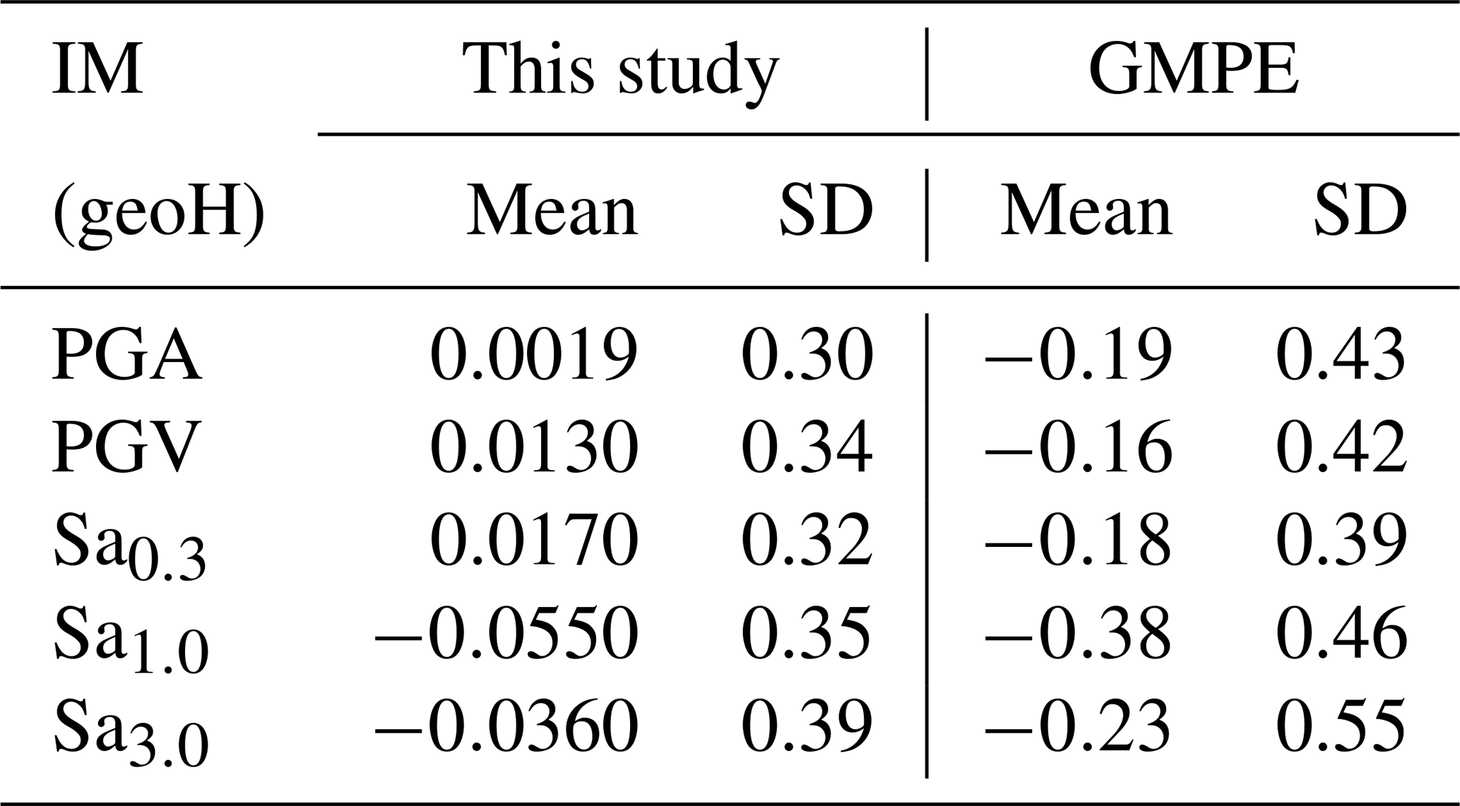

Figure 6Ground motion prediction map of Sa0.3 (resolution of 50 m × 50 m) regarding the central Italy earthquake that occurred on 24 August 2016. I_MCS values retrieved by Galli et al. (2017) are reported next to the name of the villages. Squares A and B refer to the close-ups at Arquata del Tronto and Amatrice, respectively. The surface active faulting, sketched in the figure, has been slightly modified after Galli et al. (2017).
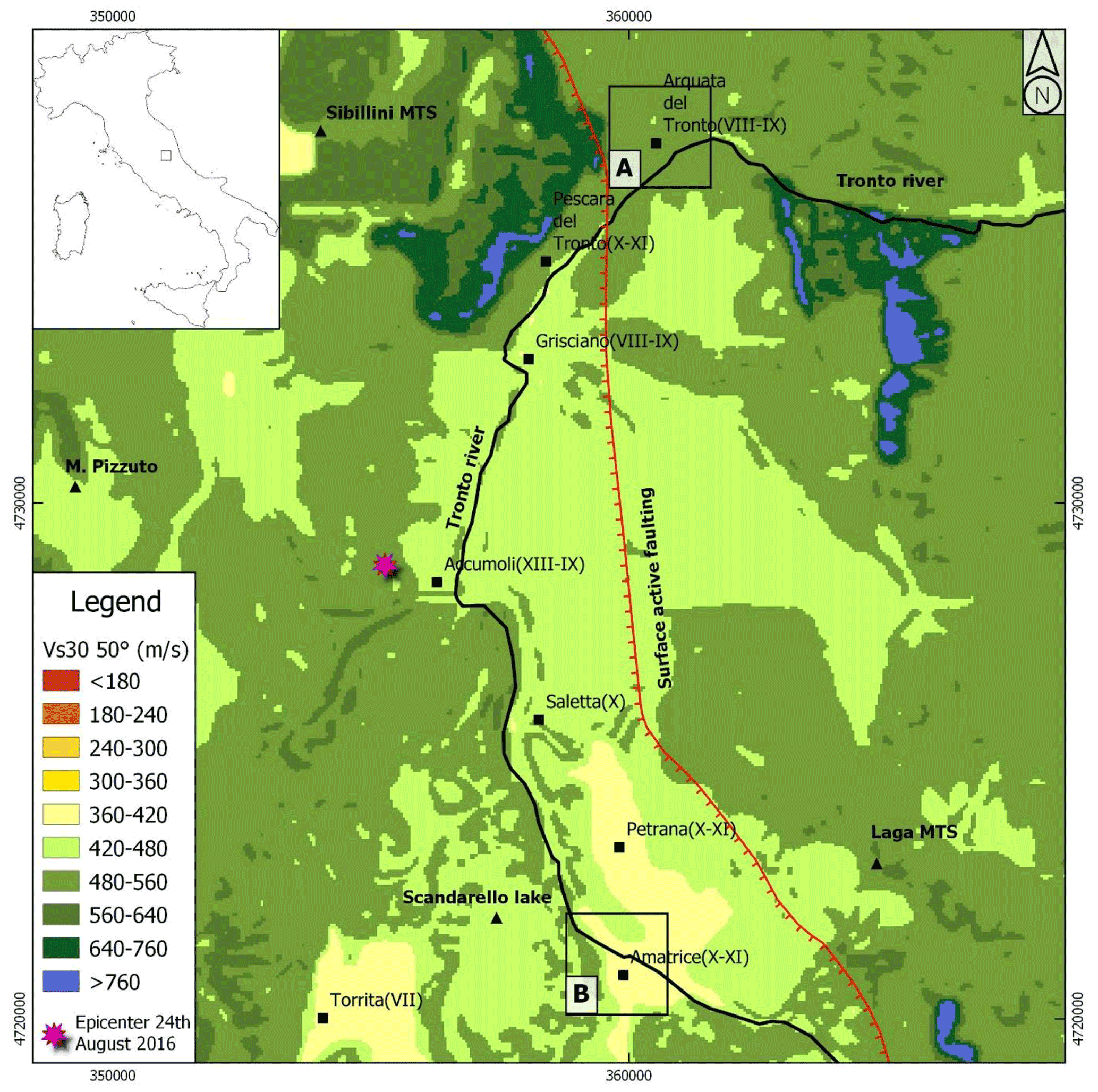
Figure 7VS30 maps for the area of interest shown in Fig. 6. It should be noted that two extended areas in the southern part of the map (i.e., near the villages of Petrana and Torrita) are characterized by the lowest values of VS30 inducing the highest Sa0.3 values (i.e., valley effect) as shown in Fig. 6.
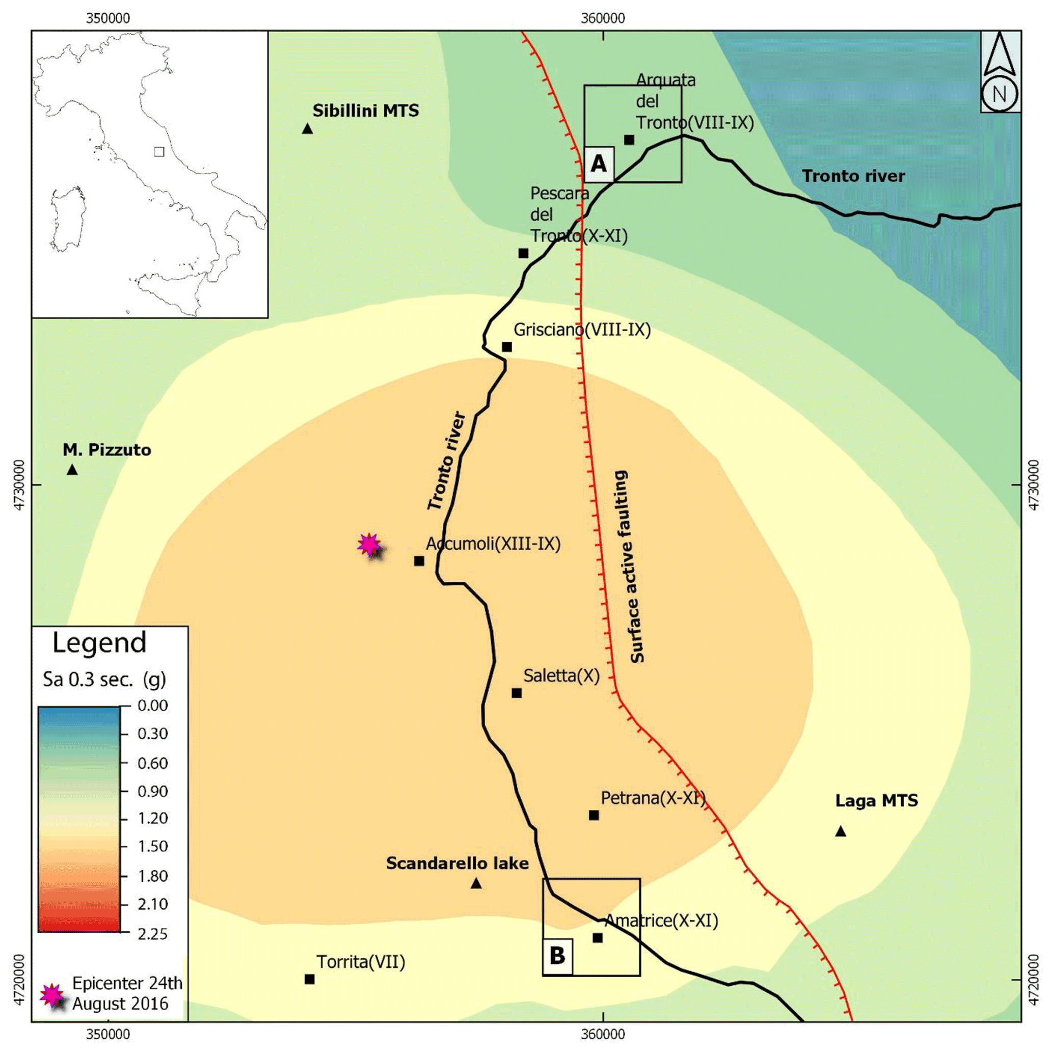
Figure 8ShakeMap (slightly modified from ShakeMap, 2021) of Sa0.3 regarding the central Italy earthquake that occurred on 24 August 2016. Squares A and B refer to the close-ups at Arquata del Tronto and Amatrice, respectively. From the center of the figure to the border, the homogenously colored areas correspond to 1.20–1.50, 0.90–1.20, 0.60–0.90, 0.30–0.60, and 0.01–0.30 g intervals. It is evident that the map does not capture the variability at short distances.
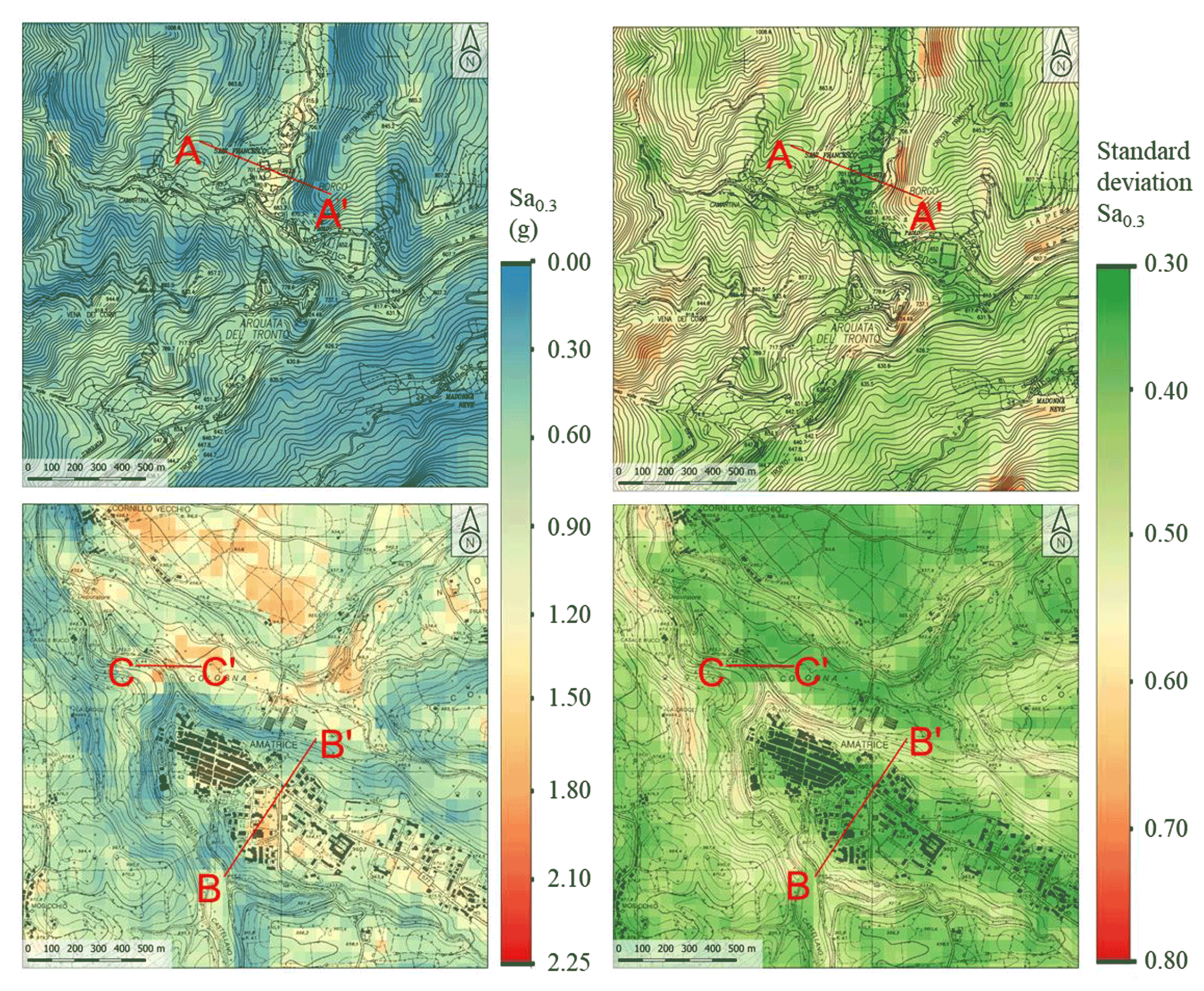
Figure 9Ground motion prediction maps (central Italy earthquake that occurred on 24 August 2016) regarding Arquata del Tronto (top) and Amatrice (bottom) in terms of the Sa0.3 mean value (left) and standard deviation (right) (resolution of 50 m × 50 m). The base topographic layer was retrieved from Regione Marche (2021) and Regione Lazio (2021) for Arquata del Tronto and Amatrice. The uncertainty estimation is available at https://it.mathworks.com/help/stats/gaussian-process-regression-models.html(last access: 1 September 2021).
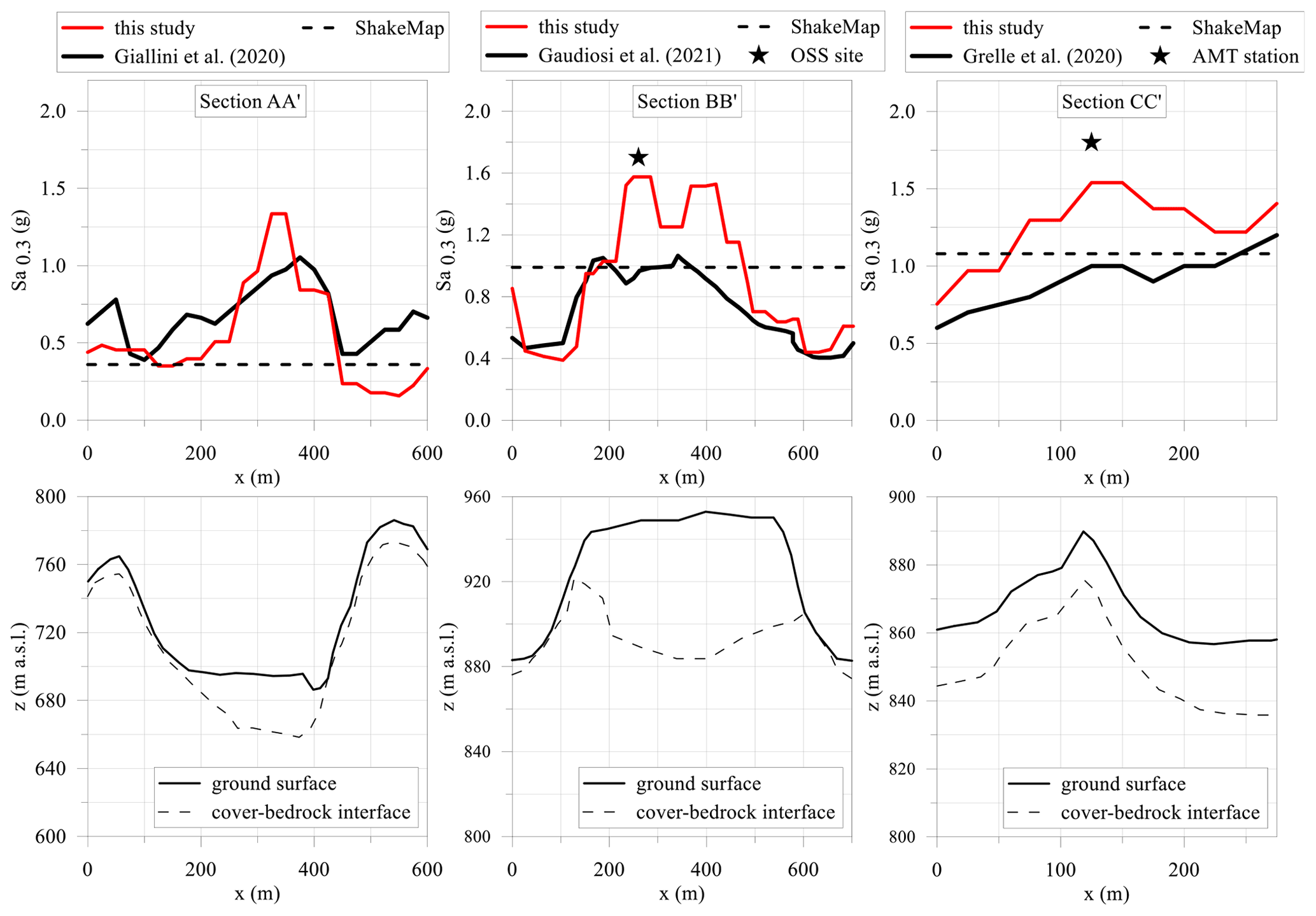
Figure 10Profiles of Sa0.3 (top) for the central Italy earthquake that occurred on 24 August 2016 and simplified subsoil sections (bottom) of Arquata del Tronto (section AA') and Amatrice (section BB' and section CC'). Cross sections' locations are in Fig. 9. Sa0.3 profiles and geological information retrieved and modified after Gaudiosi et al. (2021), Giallini et al. (2020), Grelle et al. (2020), and ShakeMap (2021). The black stars indicate values recorded at the OSS site and AMT station (for details, see the text).
After having demonstrated the goodness of the proposed method to reproduce IM values, this chapter presents examples of predictive maps produced by means of the exponential GPR model with a 50 m × 50 m resolution. In this section the map for the 24 August 2016 central Italy seismic event is produced to compare some significant IM profiles produced with independent advanced numerical simulations and data retrieved from ShakeMaps (2021).
The ground motion prediction map of the Sa0.3 reported in Fig. 6 is one of the cartographic results of this study; maps of PGA, PGV, and other spectral ordinates are in the Supplement. Macroseismic intensities, I_MCS, retrieved by Galli et al. (2017) are also reported next to the name of the villages in Fig. 6. These maps were chosen because the 0.3 s period is the fundamental vibration period of most buildings in the area (i.e., two-to-three story buildings). Moreover, 0.3 s is compatible with the results of modeling provided by Gaudiosi et al. (2021), Giallini et al. (2020), and Grelle et al. (2020) for the same areas.
The map of Fig. 6 shows an output that is in good agreement with the geophysical data (i.e., VS30 in Fig. 7) and geomorphological data (i.e., elevation and slope in Figs. A2 and A3 in Appendix A2 and A3, respectively) and, therefore, highlights local site effects. In fact, referring to Fig. 6, it should be noted that the highest Sa0.3 values describe the valleys' trend (i.e., the largest and continuous Tronto River valley) and the two extended areas in the southern part of the map (i.e., near the villages of Petrana and Torrita) well, which are characterized by the lowest values of VS30 (Mori et al., 2020a). Figure 8 shows the ShakeMap of Sa0.3 regarding the central Italy earthquake that occurred on 24 August 2016 for the same area sketched in Fig. 6. As a general issue referring to the ShakeMaps, the higher the distance from the epicenter is (the star in Fig. 8), the lower the predicted Sa0.3 is. Hence, the ShakeMaps does not provide ground motion variability induced by the local site condition (i.e., subsoil setting and topography). In detail, the ShakeMap provides an Sa0.3 value equal to 0.36 g for the entire area of Arquata del Tronto (square A in Fig. 8) and equal to 0.99 and 1.08 g for Amatrice (square B in Fig. 8).
Referring to A and B close-ups in Fig. 6, Fig. 9 shows the mean values of Sa0.3 on the left side and the standard deviation values on the right side. It should be noted that the uncertainty is provided by a combination of the input data values. The uncertainty increases referring to input data values for which the ML is not well trained (Figs. 2 and 3 and discussion in Sect. 2). For instance, standard deviation values around 0.3–0.4 are in the areas of inhabited villages, characterized by input data values widely represented in the training dataset, while values in the range of 0.6–0.8 are observed in correspondence with the combination of high slope values and high VS30 values, which are underrepresented in the training dataset.
Table 5Difference ε in percentage between Sa0.3 determined by means of different methodologies and recorded values for the central Italy earthquake that occurred on 24 August 2016.
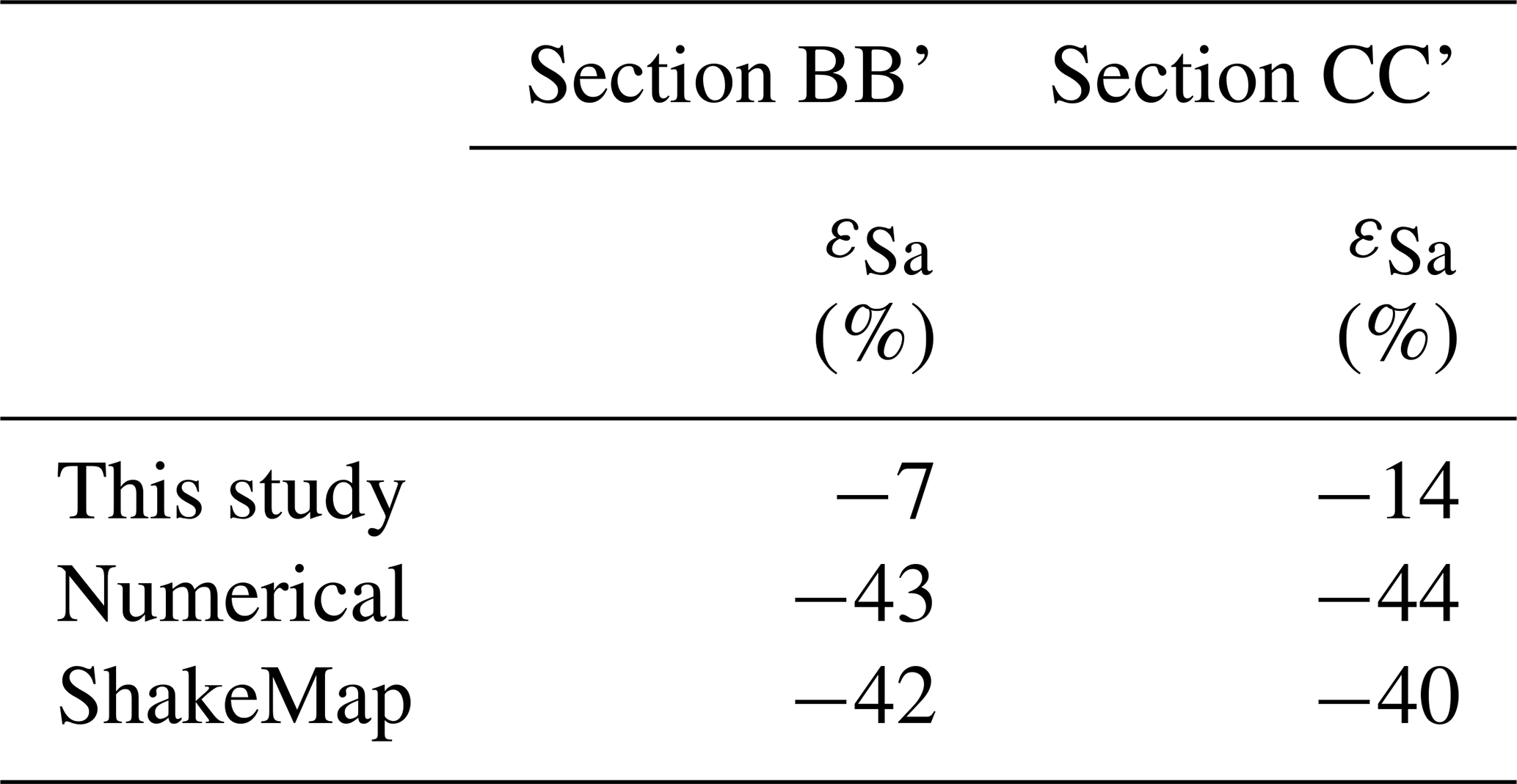
In addition to the maps, Fig. 10 shows the profiles (two at Amatrice and one at Arquata del Tronto) of Sa at 0.3 s and the comparison with the values of the same shaking parameter, calculated with different methodological approaches: ground motion prediction with an ML approach (this study), 2D numerical simulations (modified after Gaudiosi et al., 2021; Giallini et al., 2020; Grelle et al., 2020), and ShakeMap (2021). All the models are defined for the geometric mean (geoH) of the horizontal components. As ShakeMaps are released for the maximum of the horizonal components, the ShakeMap values are converted to geoH according to the empirical relation proposed by Beyer and Bommer (2006). The three profiles were chosen because they represent three very different geological and geomorphological structures: a narrow valley (section AA' in Fig. 10, Arquata del Tronto), a plateau of soft ground (section BB' in Fig. 10, Amatrice), the morphology of a mountain peak covered with soft ground (section CC' in Fig. 10, close to Amatrice). As a matter of fact, the adopted ML approach reproduces the so-called valley effect, as in the case of the Arquata del Tronto shallow valley (see the trend for m in AA'); combined lithostratigraphic and topographic effects, as in the case of the village of Amatrice (see the trend for m in BB'); and topographic amplification, as in the case of the AMT (Amatrice station code) accelerometric station (see the trend for m in CC'). It should be noted that the trend of the values of our study reproduces that of the numerical simulations and get closer to the recorded values at the Osservatorio Sismico delle Strutture (OSS, a network of buildings and bridges monitored in continuum by the Italian Civil Protection Department) site and AMT station (Luzi et al., 2019; stars in BB' and CC'). Moreover, the profiles provided by the ML approach are much more articulated and complex than the constant value (horizontal dashed line) of the ShakeMap, which obviously fails to grasp the local site effects at this scale. The difference between the different methodology and the recorded values were quantified according to the following equation and are provided in Table 5.
Intensity and frequency contents of ground motions can be altered by many factors. Up until now, numerous empirical models of ground motion amplification have been developed based on conventional regression analyses, considering a few key factors such as intensity measures of rock motions, shear-wave velocities of soils, and territory morphology. Since machine learning techniques have been applied to many fields, this work investigated on efficacy of using such techniques for developing models to predict ground motion over large areas with a 50 m resolution raster.
A set of about 16 000 ground motion data points from Italian and European networks were adopted to train a Gaussian process regression model, while recordings by 241 stations of the seismic events occurred in Italy on 30 October 2016 were used to test the same model. Peak ground acceleration and velocity, as well as spectral acceleration at three periods (i.e., 0.3, 1, and 3 s), were compared to the recorded data, allowing for obtaining residuals. With reference to the training dataset, the mean value and standard deviation of the residuals' distribution were found to equal about 0 and about 0.1, respectively. With reference to the test dataset characterized by a magnitude equal to 6.5, the mean value and standard deviation of the residuals' distribution were found to equal 0.01 and 0.3, respectively. Hence, the performance of the adopted machine learning technique was confirmed satisfactory also for a magnitude higher than 6.
In addition, maps of ground motion in terms of peak ground acceleration, peak ground velocity, and spectral acceleration at the three selected periods were produced for the central Italy seismic event that occurred on 24 August 2016. Profiles of intensity measures were in satisfactory agreement with those obtained by means of advanced numerical simulations of seismic site response referring to the same seismic event. Moreover, the adopted machine learning approach greatly improves the performance of existing methods for the analyzed case studies.
Two main novelties of the work are synthesized in the following.
-
The forecast of ground motion with high resolution (i.e., a 50 m × 50 m raster) is in agreement with results of local-scale numerical modeling. This outcome is achieved by means of machine learning techniques and large datasets including morphological, geological, geophysical, and geotechnical features (mainly the seismic-microzonation dataset; DPC, 2021). Moreover, about 1000 seismic events recorded by 1435 accelerometric stations (ESM, 2021; ITACA, 2021) were analyzed. The machine learning approach combines morphological and subsurface proxies: elevation, first- and second-order topographic gradient (defining the morphological characteristics of the territory), mean shear-wave velocity in the upper 30 m (defining the dynamic response of a site as induced by the subsoil condition), magnitude, and epicentral and hypocentral distances provide the source conditions.
-
Robust statistical techniques such as Gaussian process regression were used. Among the machine-learning-based models, the model developed by the regression and Gaussian approach provides the best performance in terms of both precision and accuracy, which are the standard deviation and mean value of the residuals' distribution, respectively.
In a nutshell, the novelty of this work is the use of the machine learning approach based on the analysis of a huge database of geological, geophysical, and geotechnical data, built with seismic-microzonation studies for the entire Italian territory. The quality and quantity of this database allow for a robust application of machine learning including the prediction of local site effects (i.e., lithostratigraphic and morphological) on the seismic ground motion.
In terms of applications, the ground motion maps generated by means of the proposed machine learning approach are useful both for urban planning (aimed at reducing seismic risk) and for emergency management (aimed at a near-real-time estimation of shaking scenarios). With reference to the emergency phase, by knowing the position and depth of the hypocenter and the magnitude of the event (in Italy these data are available a few minutes after the event), it is possible to produce ground motion maps in near real time. Overall, considering that the paradigm should be shifted from managing disasters to managing risk, the proposed methodology could represent a key tool in seismic-risk mitigation strategies deployed both before and after the seismic event.
Evaluation of the spatial-correlation structure was studied to provide the relation between local site effects and the spatial resolution of ground motion maps; results of such an analysis were not reported in the main text, since it is out of the scope of this paper, while preliminary results in terms of sill and range are reported in Appendix A4, referring to the seismic event that occurred on 30 October 2016 (i.e., the strongest of the central Italy seismic sequence).
In conclusion, the research on this topic will continue and focus on specific goals, which include the following:
-
improving the method with more input proxies which are to be made available after the seismic-microzonation project for the whole national territory (in detail, maps of the depth to the engineering bedrock and of the fundamental frequency of the deposit will be soon available and allow for using such parameters as input data for the machine learning approach)
-
improving the method with a worldwide seismological dataset
-
improving the spatial resolution of existing input proxies integrating remote sensing data
-
improving the spatial-correlation analysis.
A1 The contribution of each proxy to the total reduction in the standard deviation of the residuals for the PGA
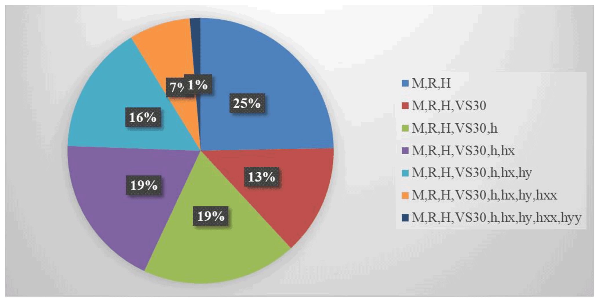
Figure A1The contribution of each proxy to the total reduction in the standard deviation of the residuals for the PGA.
A2 Elevation map for the area of Figs. 6–8
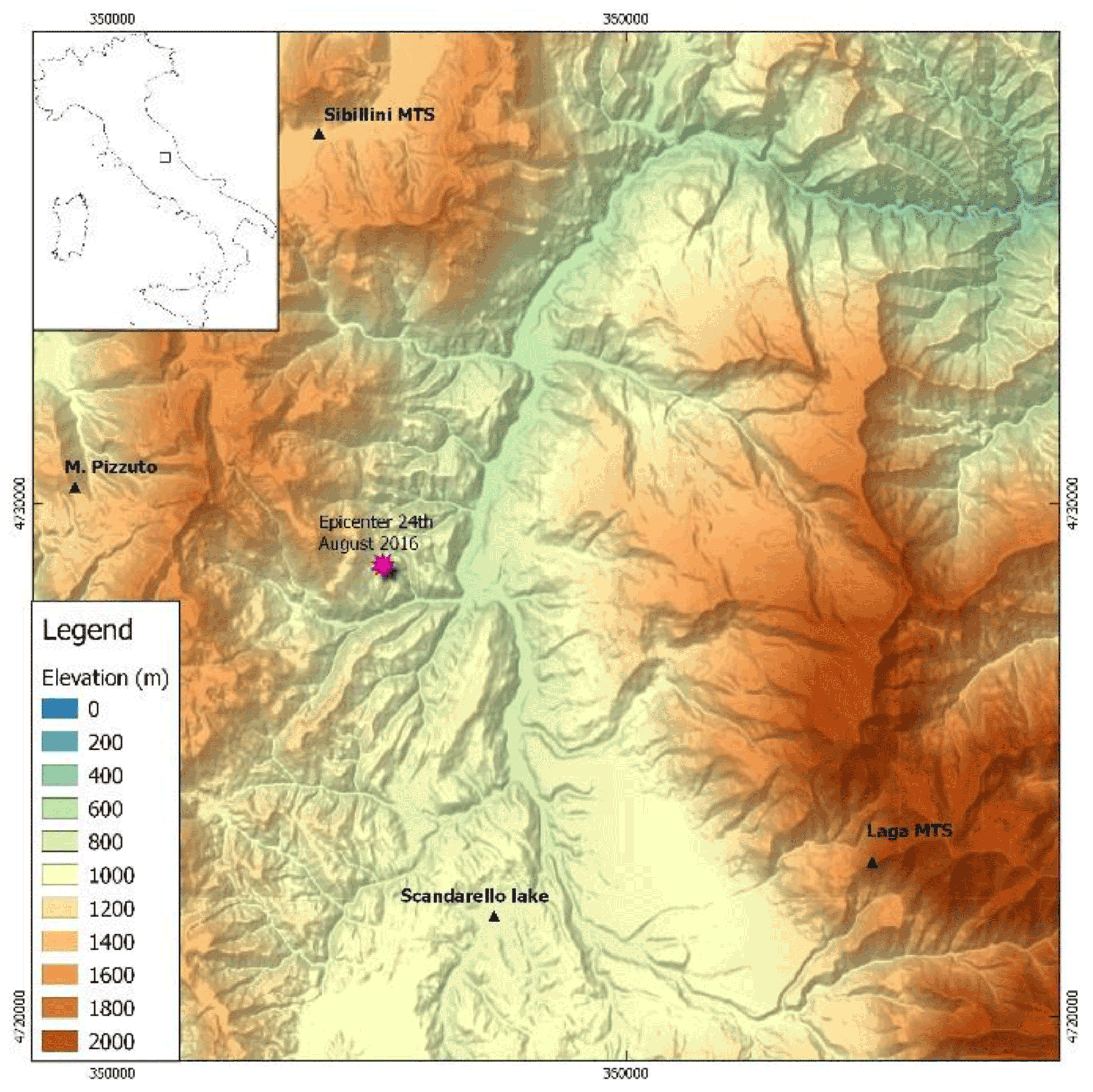
Figure A2Elevation map for the area of Figs. 6–8.
A3 Slope map for the area of Figs. 6–8
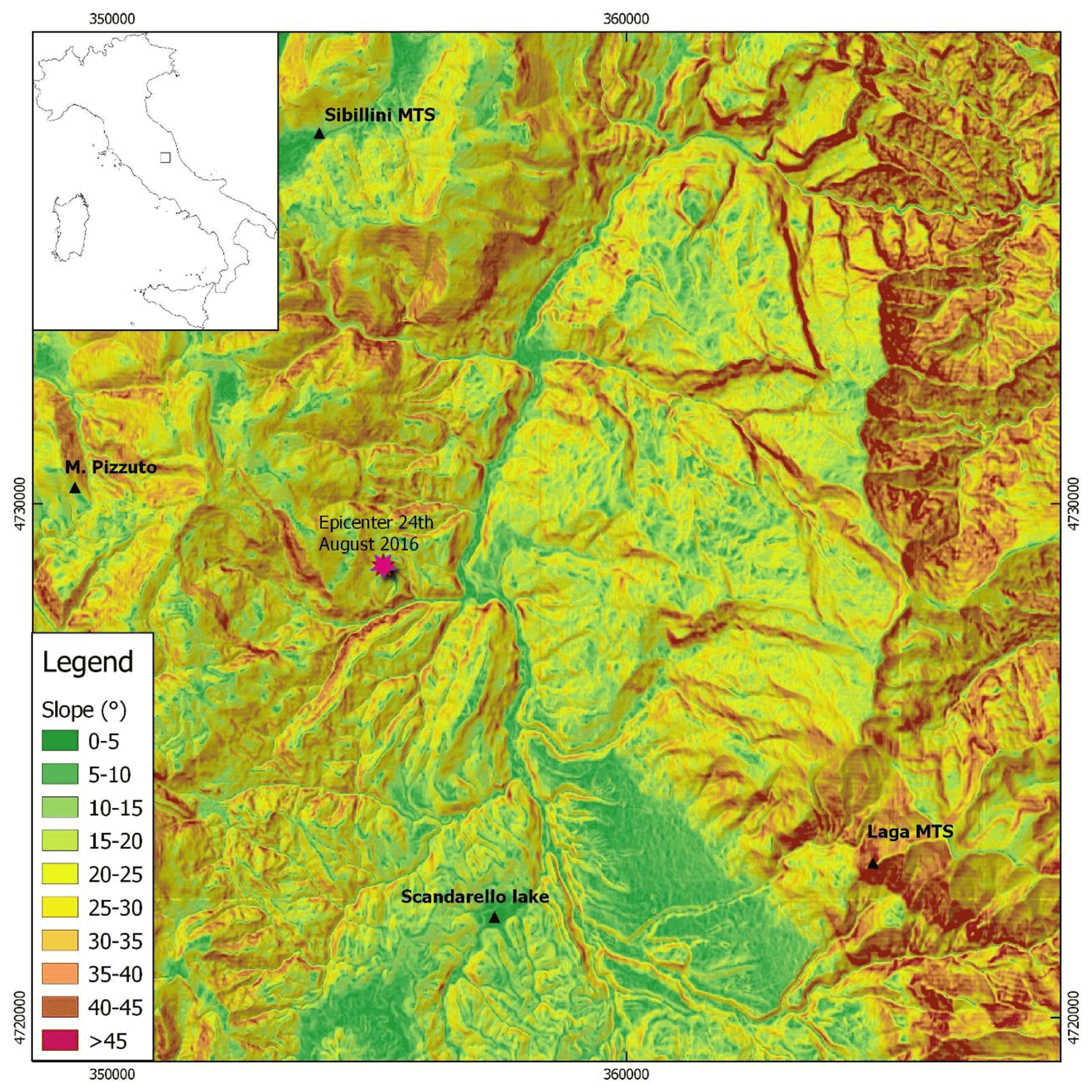
Figure A3Slope map for the area of Figs. 6–8.
A4 Spatial-correlation structure of the predicted maps
Here we want to preliminarily deal with the spatial correlation of the IM parameters. In fact, the spatial correlation of ground motion IMs represents a key issue in the seismic-risk assessment, particularly in loss analysis (Infantino et al., 2021; Schiappapietra et al., 2020, 2021). The geostatistical tool widely adopted to analyze the spatial correlation of geological and geotechnical data (Paolella et al., 2021; Raspa et al., 2008; Salvatore et al., 2019; Spacagna et al., 2018) is the semi-variogram (Chilès and Delfiner, 2012). The spatial structure is evaluated by assessing the dissimilarity of the variables measured at different locations. First, referring to the variable of interest (in this case, one of the selected IMs), the experimental semi-variogram, , is calculated from data using the method of moments (Chilès and Delfiner, 2012):
where z(xi) and z(xi+h) are the observed values of the variable z (i.e., one of the selected IMs) at the location xi and xi+h separated by h and n(h) is the number of pairs at lag h. Under the assumption of second-order stationary, the semi-variogram increases with h up to a constant value of . In this study, to assess the spatial structure of the variables (predicted IMs), the experimental variogram estimated from the predicted maps is fitted with the best-fit model (i.e., the exponential model):
where parameters a and C are called, respectively, range and sill. The range defines the correlation distance, namely, the separation distance at which the data are spatially independent, and the sill represents the variance of the random process, the limit value of γ(h).
For the central Italy event that occurred on 30 October 2016 and for all the
predicted IM maps (i.e., PGA, Sa0.3, and Sa1; see Fig. 6 and the Supplement), the spatial structure was performed with the gstat
package (Pebesma, 2004) of the R software program (R Core Team, 2021). The IM
values were extracted from the predicted maps with a regular punctual grid
of 50 m × 50 m. The isotropic experimental semi-variograms were computed and
fitted with the abovementioned exponential model. As an example, Fig. A4
shows the semi-variogram of the predicted Sa0.3 map. The spatial
structure of all predicted IM maps was characterized by the nested
exponential model. The nested variograms highlight the presence of a double
structure at different scales, i.e., a short-scale and a long-scale
variability.
In this case, two ranges and two sills are obtained for two levels of variability. Table A1 shows the sill and range values for the nested exponential models of all predicted IM maps. The first range, or short-scale structure, captures the first source of variability (first sill) over hundreds of meters induced by lithostratigraphic site conditions and morphological variability. The long-scale structure captures the variability over thousands of meters and could be referred to regional geological units and large-scale morphological features. Furthermore, a significant part of the variance, around 30 %–40 % of the total, is captured at the short scale.
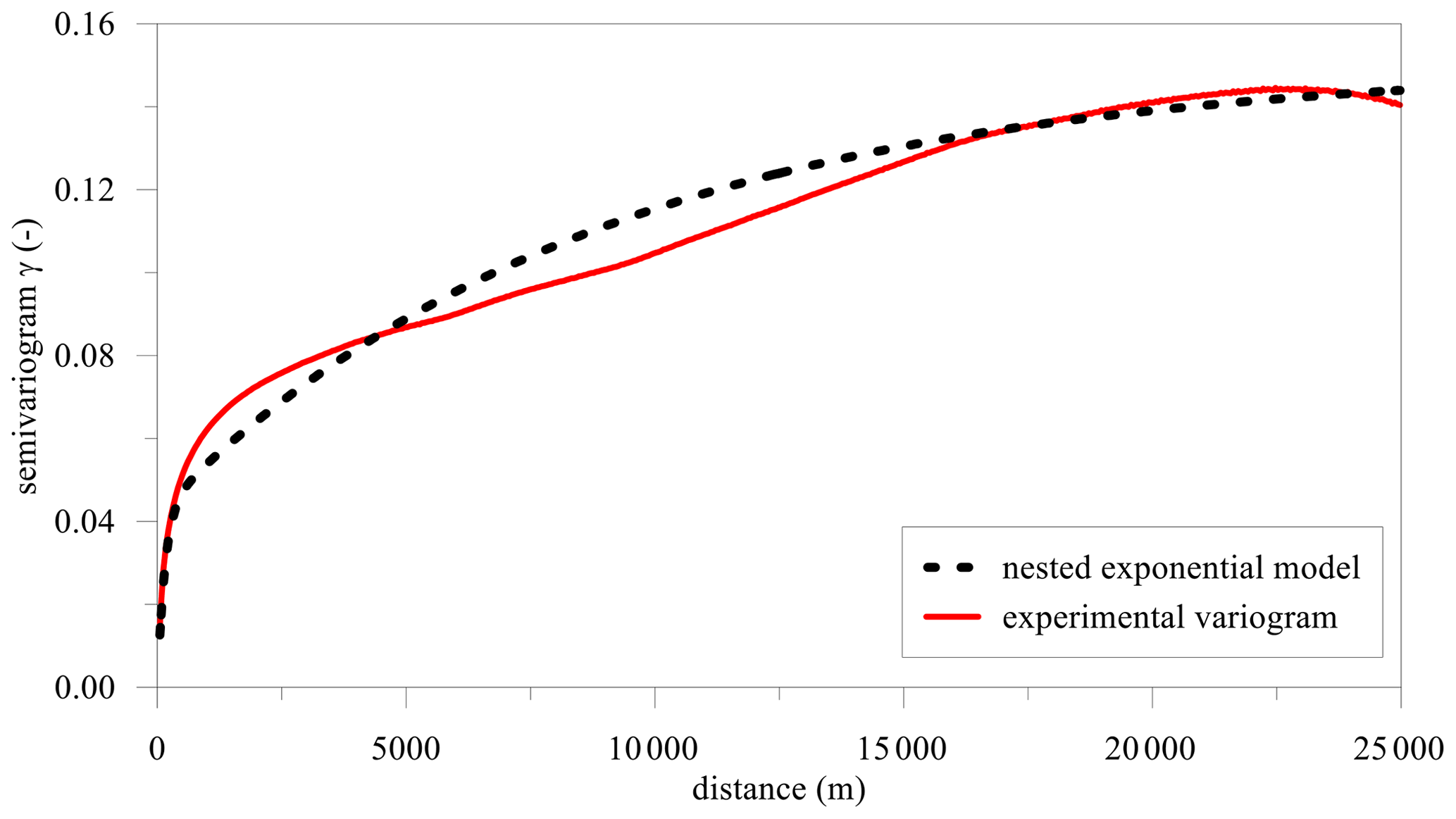
Figure A4Semi-variogram of the predicted Sa0.3 map (central Italy event that occurred on 30 October 2016): experimental variogram based on the adopted ML approach and best-fitting model (nested exponential).
Table A1Sill and range values of the nested exponential model for all the predicted IM maps.

An exhaustive treatment of this topic is beyond the scope of this work. We are now studying the spatial variability of input parameters that contribute to generate the target IM maps, and this will be the subject of a future paper. By the way, the preliminary results enlighten the importance to generate ground motion prediction maps with a spatial resolution on the order of hundreds of meters to improve their quality in terms of predictivity. Seismic-hazard maps should also include these specifications to consider the short-scale effects, even if starting from basic hazard maps with a resolution on the order of 2–5 km.
No specific code was created.
Accelerometric data are available at https://data.ingv.it/dataset/404#additional-metadata (INGV, 2022a) and https://data.ingv.it/dataset/446#additional-metadata (INGV, 2022b). Microzonation data for Italy are available at https://www.webms.it/servizi/viewer.php (Sistema Web-GIS, 2022). The VS30 map for Italy is available at https://doi.org/10.17632/8458tgzc73.1 (Mori, 2020c). The DEM is available at https://www.eorc.jaxa.jp/ALOS/en/dataset/aw3d30/aw3d30_e.htm (ALOS, 2021).
The supplement related to this article is available online at: https://doi.org/10.5194/nhess-22-947-2022-supplement.
FM and GA conceptualized the project. FM, AM, and RS curated the data. FM and RS performed the formal analysis. MM acquired funding. FM, AM, GF, GA, RS, MM, and GN conceptualized the methodology. MM administered the project. FM, MM, and GN supervised the project. FM, AM, GF, and GA validated the data. AM and GF visualized the data. FM, GF, and GN wrote the original draft of the paper. FM, AM, GF, GA, RS, MM, and GN reviewed and edited the paper.
The contact author has declared that neither they nor their co-authors have any competing interests.
Publisher’s note: Copernicus Publications remains neutral with regard to jurisdictional claims in published maps and institutional affiliations.
This article is part of the special issue “Earthquake-induced hazards: ground motion amplification and ground failures”. It is not associated with a conference.
The authors would like to thank Fabrizio Bramerini, Sergio Castenetto, Antonella Gorini, and Daniele Spina (Italian Civil Protection Department) for the useful discussions. We also thank Silvia Giallini and Iolanda Gaudiosi (both from CNR IGAG, Italy) for providing the ground motion data obtained by means of numerical simulation for the Amatrice and Arquata del Tronto areas (Italy).
This research was supported by the Presidency of the Council of Ministers of the Italian Department for Civil Protection in the framework of the project “Contratto concernente l'affidamento di servizi per il programma per il supporto al rafforzamento della Governance in materia di riduzione del rischio sismico e vulcanico ai fini di protezione civile nell'ambito del PON Governance e Capacità Istituzionale 2014–2020” (grant no. CIG6980737E65; Massimiliano Moscatelli, scientific coordinator for CNR).
This paper was edited by Hans-Balder Havenith and reviewed by four anonymous referees.
ALOS: https://www.eorc.jaxa.jp/ALOS/en/dataset/aw3d30/aw3d30_e.htm, last access: May 2021.
Beyer, K. and Bommer, J. J.: Relationships between Median Values and between Aleatory Variabilities for Different Definitions of the Horizontal Component of Motion, Bull. Seismol. Soc. Am., 96, 1512–1522, https://doi.org/10.1785/0120050210, 2006.
Bindi, D., Pacor, F., Luzi, L., Puglia, R., Massa, M., Ameri, G., and Paolucci, R.: Ground motion prediction equations derived from the Italian strong motion database, Bull. Earthq. Eng., 9, 1899–1920, https://doi.org/10.1007/s10518-011-9313-z, 2011.
Bindi, D., Massa, M., Luzi, L., Ameri, G., Pacor, F., Puglia, R., and Augliera, P.: Pan-European ground-motion prediction equations for the average horizontal component of PGA, PGV, and 5 %-damped PSA at spectral periods up to 3.0 s using the RESORCE dataset, Bull. Earthq. Eng., 12, 391–430, https://doi.org/10.1007/s10518-013-9525-5, 2014.
Bouckovalas, G. D. and Papadimitriou, A. G.: Numerical evaluation of slope topography effects on seismic ground motion, Soil Dyn. Earthq. Eng., 25, 547–558, https://doi.org/10.1016/j.soildyn.2004.11.008, 2005.
Brando, G., Pagliaroli, A., Cocco, G., and Di Buccio, F.: Site effects and damage scenarios: The case study of two historic centers following the 2016 Central Italy earthquake, Eng. Geol., 272, 105647, https://doi.org/10.1016/j.enggeo.2020.105647, 2020.
Caglar, B., Becek, K., Mekik, C., and Ozendi, M.: On the vertical accuracy of the ALOS world 3D-30 m digital elevation model, Remote Sens. Lett., 9, 607–615, https://doi.org/10.1080/2150704X.2018.1453174, 2018.
Chilès, J.-P. and Delfiner, P.: Geostatistics: modeling spatial uncertainty, 2nd edn., in: Journal of the American Statistical Association, reviewed by: Stein, M. L., Taylor and Francis, Ltd., Wiley, Hoboken, p. 726, ISBN 978-0-470-18315-1, 2012. Chiles, J.-P. and Delfiner, P.: Geostatistics: Modeling Spatial Uncertainty, J. Am. Stat. Assoc., doi:10.2307/2669569, Chilès, J. P. and Delfiner, P.: Geostatistics: Modeling Spatial Uncertainty: Second Edition., 2012.2000.
DPC (Dipartimento della Protezione Civile): Commissione tecnica per il supporto e monitoraggio degli studi di Microzonazione Sismica (ex art. 5, OPCM3907/10) – WebMs; WebCLE, edited by: Benigni, M. S., Bramerini, F., Carbone, G., Castenetto, S., Cavinato, G. P., Coltella, M., Giuffrè, M., Moscatelli, M., Naso, G., Pietrosante, A., and Stigliano, F., https://www.webms.it/, last access: May 2021.
ESM: https://esm.mi.ingv.it/, last access: May 2021.
Falcone, G., Boldini, D., and Amorosi, A.: Site response analysis of an urban area: A multi-dimensional and non-linear approach, Soil Dyn. Earthq. Eng., 109, 33–45, https://doi.org/10.1016/J.SOILDYN.2018.02.026, 2018.
Falcone, G., Romagnoli, G., Naso, G., Mori, F., Peronace, E., and Moscatelli, M.: Effect of bedrock stiffness and thickness on numerical simulation of seismic site response. Italian case studies, Soil Dyn. Earthq. Eng., 139, 106361, https://doi.org/10.1016/j.soildyn.2020.106361, 2020a.
Falcone, G., Boldini, D., Martelli, L., and Amorosi, A.: Quantifying local seismic amplification from regional charts and site specific numerical analyses: a case study, Bull. Earthq. Eng., 18, 77–107, https://doi.org/10.1007/s10518-019-00719-9, 2020b.
Falcone, G., Acunzo, G., Mendicelli, A., Mori, F., Naso, G., Peronace, E., Porchia, A., Romagnoli, G., Tarquini, E., and Moscatelli, M.: Seismic amplification maps of Italy based on site-specific microzonation dataset and one-dimensional numerical approach, Eng. Geol., 289, 106170, https://doi.org/10.1016/j.enggeo.2021.106170, 2021.
Fayjaloun, R., Negulescu, C., Roullé, A., Auclair, S., Gehl, P., Faravelli, M., Abrahamczyk, L., Petrovčič, S., and Martinez-Frias, J.: Sensitivity of Earthquake Damage Estimation to the Input Data (Soil Characterization Maps and Building Exposure): Case Study in the Luchon Valley, France, Geosci., 11, 249, https://doi.org/10.3390/geosciences11060249, 2021.
Galli, P., Castenetto, S., and Peronace, E.: The Macroseismic Intensity Distribution of the 30 October 2016 Earthquake in Central Italy (Mw6.6): Seismotectonic Implications, Tectonics, 36, 2179–2191, https://doi.org/10.1002/2017TC004583, 2017.
Gatmiri, B. and Arson, C.: Seismic site effects by an optimized 2D BE/FE method II. Quantification of site effects in two-dimensional sedimentary valleys, Soil Dyn. Earthq. Eng., 28, 646–661, https://doi.org/10.1016/J.SOILDYN.2007.09.002, 2008.
Gaudiosi, I., Simionato, M., Mancini, M., Cavinato, G. P., Coltella, M., Razzano, R., Sirianni, P., Vignaroli, G., and Moscatelli, M.: Evaluation of site effects at Amatrice (central Italy) after the August 24th, 2016, Mw6.0 earthquake, Soil Dyn. Earthq. Eng., 144, 106699, https://doi.org/10.1016/j.soildyn.2021.106699, 2021.
Gazetas, G.: Vibrational characteristics of soil deposits with variable wave velocity, Int. J. Numer. Anal. Methods Geomech., 6, 1–20, https://doi.org/10.1002/nag.1610060103, 1982.
Giallini, S., Pizzi, A., Pagliaroli, A., Moscatelli, M., Vignaroli, G., Sirianni, P., Mancini, M., and Laurenzano, G.: Evaluation of complex site effects through experimental methods and numerical modelling: The case history of Arquata del Tronto, central Italy, Eng. Geol., 272, 105646, https://doi.org/10.1016/j.enggeo.2020.105646, 2020.
Grelle, G., Gargini, E., Facciorusso, J., Maresca, R., and Madiai, C.: Seismic site effects in the Red Zone of Amatrice hill detected via the mutual sustainment of experimental and computational approaches, Bull. Earthq. Eng., 18, 1955–1984, https://doi.org/10.1007/s10518-019-00777-z, 2020.
Infantino, M., Smerzini, C., and Lin, J.: Spatial correlation of broadband ground motions from physics-based numerical simulations, Earthquake Eng. Struct. Dyn., 2021, 1–20, 2021.
Istituto Nazionale di Geofisica e Vulcanologia (INGV): Engineering Strong Motion Database (ESM) flatfile, INGV [data set], https://data.ingv.it/dataset/404#additional-metadata (last access: September 2021), 2022a.
Istituto Nazionale di Geofisica e Vulcanologia (INGV): NEar-Source Strong-motion flatfile (NESS), version 2.0, INGV [data set], https://data.ingv.it/dataset/446#additional-metadata, (last access: September 2021), 2022b.
ITACA: http://itaca.mi.ingv.it/ItacaNet_30/#/home, last access: May 2021.
Iwahashi, J., Kamiya, I., Matsuoka, M., and Yamazaki, D.: Global terrain classification using 280 m DEMs: segmentation, clustering, and reclassification, Prog. Earth Planet. Sci., 5, 1, https://doi.org/10.1186/s40645-017-0157-2, 2018.
Jozinović, D., Lomax, A., Štajduhar, I., and Michelini, A.: Rapid prediction of earthquake ground shaking intensity using raw waveform data and a convolutional neural network, Geophys. J. Int., 222, 1379–1389, https://doi.org/10.1093/GJI/GGAA233, 2021.
Kim, S., Hwang, Y., Seo, H., and Kim, B.: Ground motion amplification models for Japan using machine learning techniques, Soil Dyn. Earthq. Eng., 132, 106095, https://doi.org/10.1016/j.soildyn.2020.106095, 2020.
Kubo, H., Kunugi, T., Suzuki, W., Suzuki, S., and Aoi, S.: Hybrid predictor for ground-motion intensity with machine learning and conventional ground motion prediction equation, Sci. Rep., 10, 11871, https://doi.org/10.1038/s41598-020-68630-x, 2020.
Luo, Y., Fan, X., Huang, R., Wang, Y., Yunus, A. P., and Havenith, H. B.: Topographic and near-surface stratigraphic amplification of the seismic response of a mountain slope revealed by field monitoring and numerical simulations, Eng. Geol., 271, 105607, https://doi.org/10.1016/j.enggeo.2020.105607, 2020.
Luzi, L., Puglia, R., Russo, E., and ORFEUS WG5: Engineering Strong Motion Database, version 1.0. Istituto Nazionale di Geofisica e Vulcanologia [data set], Observatories & Research Facilities for European Seismology, https://doi.org/10.13127/ESM, 2016.
Luzi, L., Pacor, F., and Puglia, R.: Italian Accelerometric Archive v3.0, Istituto Nazionale di Geofisica e Vulcanologia, Dipartimento della Protezione Civile Nazionale [data set], https://doi.org/10.13127/itaca.3.0, 2019.
Luzi, L., Lanzano, G., Felicetta, C., D'Amico, M. C., Russo, E., Sgobba, S., Pacor, F., and ORFEUS Working Group 5: Engineering Strong Motion Database (ESM) (Version 2.0), Istituto Nazionale di Geofisica e Vulcanologia (INGV) [data set], https://doi.org/10.13127/ESM.2, 2020.
MathWorks: Statistics and Machine Learning Toolbox User's Guide R2019b, The MATLAB MathWorks Inc., Natick, MA, USA, 2019.
Michelini, A., Faenza, L., Lanzano, G., Lauciani, V., Jozinović, D., Puglia, R., and Luzi, L.: The new shakemap in Italy: Progress and advances in the last 10 yr, Seismol. Res. Lett., 91, 317–333, https://doi.org/10.1785/0220190130, 2019.
Mori, F., Gaudiosi, I., Tarquini, E., Bramerini, F., Castenetto, S., Naso, G., and Spina, D.: HSM: a synthetic damage-constrained seismic hazard parameter, Bull. Earthq. Eng., 18, 5631–5654, https://doi.org/10.1007/s10518-019-00677-2, 2019.
Mori, F., Mendicelli, A., Moscatelli, M., Romagnoli, G., Peronace, E., and Naso, G.: A new Vs30 map for Italy based on the seismic microzonation dataset, Eng. Geol., 275, 105745, https://doi.org/10.1016/j.enggeo.2020.105745, 2020a.
Mori, F., Gena, A., Mendicelli, A., Naso, G., and Spina, D.: Seismic emergency system evaluation: The role of seismic hazard and local effects, Eng. Geol., 270, 105587, https://doi.org/10.1016/j.enggeo.2020.105587, 2020b.
Mori, F., Mendicelli, A., Moscatelli, M., Romagnoli, G., Peronace, E., and Naso, G.: “Data for: A new Vs30 map for Italy based on the seismic microzonation dataset”, Mendeley Data [data set], https://doi.org/10.17632/8458tgzc73.1, 2020c.
Moscatelli, M., Albarello, D., Scarascia Mugnozza, G., and Dolce, M.: The Italian approach to seismic microzonation, Bull. Earthq. Eng., 18, 5425–5440, https://doi.org/10.1007/s10518-020-00856-6, 2020a.
Moscatelli, M., Vignaroli, G., Pagliaroli, A., Razzano, R., Avalle, A., Gaudiosi, I., Giallini, S., Mancini, M., Simionato, M., Sirianni, P., Sottili, G., Bellanova, J., Calamita, G., Perrone, A., Piscitelli, S., and Lanzo, G.: Physical stratigraphy and geotechnical properties controlling the local seismic response in explosive volcanic settings: the Stracciacappa maar (central Italy), Bull. Eng. Geol. Environ., 80, 179–199 https://doi.org/10.1007/s10064-020-01925-5, 2020b.
Pagani, M., Monelli, D., Weatherill, G., Danciu, L., Crowley, H., Silva, V., Henshaw, P., Butler, L., Nastasi, M., Panzeri, L., Simionato, M., and Vigano, D.: OpenQuake Engine: An Open Hazard (and Risk) Software for the Global Earthquake Model, Seismol. Res. Lett., 85, 692–702, https://doi.org/10.1785/0220130087, 2014.
Pagliaroli, A., Moscatelli, M., Raspa, G., and Naso, G.: Seismic microzonation of the central archaeological area of Rome: results and uncertainties, Bull. Earthq. Eng., 12, 1405–1428, https://doi.org/10.1007/s10518-013-9480-1, 2014.
Pebesma, E. J.: Multivariable geostatistics in S: the gstat package, Comput. Geosci., 30, 683–691, 2004.
Paolella, L., Spacagna, R. L., Chiaro, G., and Modoni, G.: A simplified vulnerability model for the extensive liquefaction risk assessment of buildings, B. Earthq. Eng., 19, 3933–3961, 2021.
Pitilakis, K., Raptakis, D., Lontzetidis, K., Tika-Vassilikou, T., and Jongmans, D.: Geotechnical and geophysical description of euro-seistest, using field, laboratory tests and moderate strong motion recordings, J. Earthq. Eng., 3, 381–409, https://doi.org/10.1080/13632469909350352, 1999.
R Core Team: R: A language and environment for statistical computing, R Foundation for Statistical Computing, Vienna, Austria, https://www.R-project.org/, last access: 1 September 2021.
Rasmussen, C. E. and Williams, C. K. I.: Gaussian Processes for Machine Learning, MIT Press, Massachusetts Institute of Technology, 266 pp., http://www.gaussianprocess.org/gpml/chapters/RW.pdf (last access: 17 March 2022), 2006.
Raspa, G., Moscatelli, M., Stigliano, F. P., Patera, A., Folle, D., Vallone, R., Mancini, M., Cavinato, G. P., Milli, S., and Costa J. F. C. L.: Geotechnical characterization of the upper Pleistocene-Holocene alluvial deposits of Roma (Italy) by means of multivariate geostatistics: crossvalidation results, Eng. Geol., 101, 251–268, https://doi.org/10.1016/j.enggeo.2008.06.007, 2008.
Regione Lazio: https://sciamlab.com/opendatahub/dataset/r_lazio_carta-tecnica-regionale-1991, last access: May 2021.
Regione Marche: https://www.regione.marche.it/Regione-Utile/Paesaggio-Territorio-Urbanistica/Cartografia/Repertorio/Cartatecnicanumerica110000, last access: May 2021.
Régnier, J., Bonilla, L., Bard, P., Bertrand, E., Hollender, F., Kawase, H., Sicilia, D., Arduino, P., Amorosi, A., Asimaki, D., Boldini, D., Chen, L., Chiaradonna, A., DeMartin, F., Ebrille, M., Elgamal, A., Falcone, G., Foerster, E., Foti, S., Garini, E., Gazetas, G., Gélis, C., Ghofrani, A., Giannakou, A., Gingery, J. R., Glinsky, N., Harmon, J., Hashash, Y., Iai, S., Jeremić, B., Kramer, S., Kontoe, S., Kristek, J., Lanzo, G., Lernia, A. di, Lopez-Caballero, F., Marot, M., McAllister, G., Diego Mercerat, E., Moczo, P., Montoya-Noguera, S., Musgrove, M., Nieto-Ferro, A., Pagliaroli, A., Pisanò, F., Richterova, A., Sajana, S., Santisi d'Avila, M. P., Shi, J., Silvestri, F., Taiebat, M., Tropeano, G., Verrucci, L., and Watanabe, K.: International Benchmark on Numerical Simulations for 1D, Nonlinear Site Response (PRENOLIN): Verification Phase Based on Canonical Cases, Bull. Seismol. Soc. Am., 106, 2112–2135, https://doi.org/10.1785/0120150284, 2016.
Régnier, J., Bonilla, L., Bard, P., Bertrand, E., Hollender, F., Kawase, H., Sicilia, D., Arduino, P., Amorosi, A., Asimaki, D., Boldini, D., Chen, L., Chiaradonna, A., DeMartin, F., Elgamal, A., Falcone, G., Foerster, E., Foti, S., Garini, E., Gazetas, G., Gélis, C., Ghofrani, A., Giannakou, A., Gingery, J., Glinsky, N., Harmon, J., Hashash, Y., Iai, S., Kramer, S., Kontoe, S., Kristek, J., Lanzo, G., Lernia, A. di, Lopez-Caballero, F., Marot, M., McAllister, G., Diego Mercerat, E., Moczo, P., Montoya-Noguera, S., Musgrove, M., Nieto-Ferro, A., Pagliaroli, A., Passeri, F., Richterova, A., Sajana, S., Santisi d'Avila, M. P., Shi, J., Silvestri, F., Taiebat, M., Tropeano, G., Vandeputte, D., and Verrucci, L.: PRENOLIN: International Benchmark on 1D Nonlinear Site-Response Analysis–Validation Phase Exercise, Bull. Seismol. Soc. Am., 108, 876–900, https://doi.org/10.1785/0120170210, 2018.
Salvatore, E., Spacagna, R. L., Andò, E., and Ochmanski, M.: Geostatistical analysis of strain localization in triaxial tests on sand, Geotech. Lett., 9, 334–339, https://doi.org/10.1680/jgele.18.00228, 2019.
Schiappapietra, E. and Douglas, J.: Modelling the spatial correlation of earthquake ground motion: Insights from the literature, data from the 2016–2017 Central Italy earthquake sequence and ground-motion simulations, Earth-Sci. Rev., 203, 103139, https://doi.org/10.1016/j.earscirev.2020.103139, 2020.
Schiappapietra, E. and Smerzini, C.: Spatial correlation of broadband earthquake ground motion in Norcia (Central Italy) from physics-based simulations, Bull. Earthq. Eng., 19, 4693–4717, https://doi.org/10.1007/s10518-021-01160-7, 2021.
ShakeMap: http://shakemap.rm.ingv.it/shake4/, last access: May 2021.
Sistema Web-GIS: Portale cartografico della Microzonazione Sismica e della Condizione Limite per l'Emergenza, https://www.webms.it/servizi/viewer.php (last access: September 2021), 2022.
SM Working Group: Guidelines for Seismic Microzonation, Conference of Regions and Autonomous Provinces of Italy – Civil Protection Department, Rome, 3 Vol. and DVD, https://www.centromicrozonazionesismica.it/it/download/category/9-guidelines-for-seismic-microzonation (last access: 1 September 2021), 2008.
Spacagna, R. L. and Modoni, G.: GIS-based study of land subsidence in the city of Bologna, Mechatronics for Cultural Heritage and Civil Engineering, 92, 235–256, https://doi.org/10.1007/978-3-319-68646-2_10, 2018.
Tamhidi, A., Kuehn, N., Ghahari, S. F., Rodgers, A. J., Kohler, M. D., Taciroglu, E., and Bozorgnia, Y.: Conditioned Simulation of Ground-Motion Time Series at Uninstrumented Sites Using Gaussian Process Regression, B. Seismol. Soc. Am., 112, 331–347, https://doi.org/10.1785/0120210054, 2021.
TCSM: Technical Commission for Seismic Microzonation. Graphic and Data Archiving Standards, Version 4.1, National Department of Civil Protection, Rome, https://www.centromicrozonazionesismica.it/it/download/send/26-standardms-41/71-standardms-4-1 (last access: 1 September 2021), 2018.
Wald, D. J., Worden, C. B., Thompson, E. M., and Hearne, M.: ShakeMap operations, policies, and procedures, Earthq. Spectra, 38, 756–777, https://doi.org/10.1177/87552930211030298, 2021.
Zhou, H., Li, J., and Chen, X.: Establishment of a seismic topographic effect prediction model in the Lushan Ms7.0 earthquake area, Geophys. J. Int., 221, 273–288, https://doi.org/10.1093/gji/ggaa003, 2020.
- Abstract
- Introduction
- Input and output data for machine learning training and validation
- Seismological parameters
- Geophysical data
- Morphological data
- Method
- Ground motion prediction map for the central Italy seismic event that occurred on 24 August 2016 and comparison with numerical modeling
- Discussion and conclusions
- Appendix A: Spatial-correlation structure of the predicted maps and some clarifications requested during the revision phase
- Code availability
- Data availability
- Author contributions
- Competing interests
- Disclaimer
- Special issue statement
- Acknowledgements
- Financial support
- Review statement
- References
- Supplement