Automated determination of landslide locations after large trigger events: advantages and disadvantages compared to manual mapping

Earthquakes in mountainous areas can trigger thousands of co-seismic landslides, causing significant damage, hampering relief efforts, and rapidly redistributing sediment across the landscape. Efforts to understand the controls on these landslides rely heavily on manually mapped landslide inventories, but these are costly and time-consuming to collect, and their reproducibility is not typically well constrained. Here we develop a new automated landslide detection index (ALDI) algorithm based on pixel-wise normalised difference vegetation index (NDVI) differencing of Landsat time series within Google Earth Engine accounting for seasonality. We compare classified inventories to manually mapped inventories from five recent earthquakes: Kashmir in 2005, Aysén in 2007, Wenchuan in 2008, Haiti in 2010, and Gorkha in 2015. We test the ability of ALDI to recover landslide locations (using receiver operating characteristic – ROC – curves) and landslide sizes (in terms of landslide area–frequency statistics). We find that ALDI more skilfully identifies landslide locations than published inventories in 10 of 14 cases when ALDI is locally optimised and in 8 of 14 cases both when ALDI is globally optimised and in holdback testing. These results reflect not only good performance of the automated approach but also surprisingly poor performance of manual mapping, which has implications both for how future classifiers are tested and for the interpretations that are based on these inventories. We find that manual mapping, which typically uses finer-resolution imagery, more skilfully captures the landslide area–frequency statistics, likely due to reductions in both the censoring of individual small landslides and amalgamation of landslide clusters relative to ALDI. We conclude that ALDI is a viable alternative to manual mapping in terms of its ability to identify landslide-affected locations but is less suitable for detecting small isolated landslides or precise landslide geometry. Its fast run time, cost-free image requirements, and near-global coverage suggest the potential to significantly improve the coverage and quantity of landslide inventories. Furthermore, its simplicity (pixel-wise analysis only) and parsimony of inputs (optical imagery only) mean that considerable further improvement should be possible.

1 Introduction

Landslides are important as both agents of erosion and as a dangerous hazard (Marc et al., 2016; Froude and Petley, 2018). Large earthquakes or rainstorms can trigger thousands of landslides, redistributing tonnes of rock over distances of hundreds or thousands of metres within a few seconds (Li et al., 2014; Roback et al., 2018). These landslides can cause significant damage, hamper relief efforts, and rapidly redistribute sediment across the landscape. Efforts to understand the drivers, behaviour, and consequences of these landslides rely heavily on landslide inventories, in which landslide locations are mapped either as points, pixels, or polygons, usually associated with one or more assumed trigger events. Landslide inventories are important because they document the extent and impact of landslides in a region, informing disaster response and recovery (Williams et al., 2018); they capture the distribution, properties, and (through predictive models) drivers of landslides (Guzzetti et al., 2012; Tanyaş et al., 2019); they can be used to train and evaluate models of landslide susceptibility, hazard, and risk (Van Westen et al., 2006; Reichenbach et al., 2018); and they enable geophysical flux calculations central to the study of landscape evolution and the global carbon cycle (e.g. Hilton et al., 2008; Marc et al., 2016; Dietrich et al., 2003).

Polygon-based and pixel-based inventories both capture information on the area affected by landslide movement. Polygon-based inventories have the additional advantage that they can be analysed to yield distributions of landslide geometry (such as area and shape), which is useful for understanding fluxes of material (Larsen et al., 2010) or impact forces and distinguishing scars from runout areas (Marc et al., 2018).

Landslide inventories were traditionally generated from expensive and time-consuming site visits (e.g. Warburton et al., 2008), severely limiting the number of landslides that could be mapped and thus the scale of enquiry. However, they are now increasingly collected remotely based on interpretation of satellite or aerial imagery, which enables much larger datasets to be compiled (e.g. Li et al., 2014; Roback et al., 2018).

Imagery provides an opportunity for rapid mapping over wide areas but is subject to some important limitations. For optical imagery, which depends on reflected solar energy reaching the sensor, clouds and shadows can obscure the ground surface. Active sensors, such as radar, that operate at wavelengths that are not reflected by cloud suffer from other issues (e.g. radar layover and shadowing), and their images have only recently been incorporated into operational landslide mapping approaches (e.g. Konishi and Suga, 2018; Burrows et al., 2019; Aimaiti et al., 2019; Mondini et al., 2019). Images may not be available for the study area over the time window of interest, and – when they are available – they can be costly to acquire. In steep or high-relief topography, images can suffer severe georectification errors (Williams et al., 2018), which is particularly problematic for landslide mapping because these are the areas of most interest. Imagery is becoming increasingly available across a very wide range of spatial and spectral resolutions, but there remains a trade-off between resolution and cost, with 10–30 m imagery freely available globally with a 14 d revisit time (e.g. Sentinel-2, Landsat 8), while sub-metric resolution data (e.g. WorldView, Pléiades) can be acquired on demand but at a cost of USD 10–10 000 per square kilometre.

Landslides are typically identified in imagery either by automated classification, manual mapping, or some hybrid of the two. Manual mapping, although much faster than site visits, remains very time-consuming over moderate to large areas (Galli et al., 2008), particularly for co-seismic inventories, which can involve digitising 10⁴ to 10⁵ landslides (e.g. Xu et al., 2014; Harp et al., 2016). It also requires a comparison of pre- and post-event images to identify change and to avoid conflation of landslides related to the trigger event with those occurring before or after the event (e.g. Hovius et al., 2011; Marc et al., 2015). Automated classification can considerably speed up this process but is complicated by other factors, including the range of possible landslide sizes and geometries; the non-unique signatures of landslides relative to roads, buildings, or other features; and the difficulty of excluding pre-existing landslides (Parker et al., 2011; Behling et al., 2014). Automated landslide classification has been demonstrated predominantly using high-resolution imagery and requires a high level of tuning; thus it is not necessarily transferrable from one region or event to another. Imagery can be combined with other sources of information (e.g. slope inclination from digital elevation models, DEMs) to remove some false positives, where a location is incorrectly classified as a landslide (Parker et al., 2011). This can improve classifier performance but can also generate spurious correlation when interpreting the results (e.g. landslide susceptibility with slope inclination). Some authors have adopted hybrid approaches; for example, Li et al. (2014) applied manual checking to the earlier automated mapping of Parker et al. (2011).

As a result of these issues, our database of landslide inventories is limited in number and biased towards the most spectacular trigger events. This point is most easily illustrated by examining earthquake-triggered landslide inventories, since in this case the trigger event is generally very clearly identifiable in time, and its footprint is well defined in space. Of the 326 earthquakes known to have triggered landslides between 1976 and 2016, only 46 have published landslide maps (Tanyaş et al., 2017). For 225 earthquakes the existence of co-seismic landslides was known from news reports and witness testimony (Marano et al., 2010), but no reliable quantitative or spatial landslide data are available (Tanyaş et al., 2017). Many other earthquakes have likely triggered landslides, but these have gone unreported because they occurred out of human view. Between 1976 and 2016 there were ∼6500 earthquakes sufficiently large (> M_w 5), shallow (< 25 km), and near to land (< 25 km) to trigger landslides (based on Marc et al., 2016). This suggests that the existing set of co-seismic landslide inventories is a small subset (< 15 %) of those earthquakes known to have triggered landslides and a tiny subset (< 1 %) of those likely to have triggered landslides.

Extending the number of landslide inventories requires a reduction in the cost of inventory collection, both in terms of imagery expense and mapping time. We hypothesise that recent improvements in satellite data management (e.g. data cubes) and computing capabilities (e.g. cloud computing) have made it possible to collect automated landslide inventories of comparable quality to manual mapping, at a fraction of the cost, due to reductions in both imagery cost and mapping time. Imagery cost could be reduced by using cheaper, lower-resolution imagery, while mapping time could be reduced by using automated detection rather than manual mapping. However, these savings will only represent value for money if they can deliver inventories of comparable or superior quality to manual mapping.

Large amounts of freely available optical imagery with near-global coverage have been generated by the Landsat and Sentinel programmes. Landsat has been running for more than 30 years (since the Landsat 4 launch in 1982), imaging the majority of Earth's surface at a return time of ca. 14 d and at 30 m spatial resolution through the visible and infrared bands. Landsat received early attention as a source of imagery for manual landslide mapping (e.g. Sauchyn and Trench, 1978; Greenbaum et al., 1995) but has since been largely superseded by imagery with higher spatial resolution, which is often assumed to result in more precise inventories (e.g. Parker et al., 2011; Li et al., 2014; Roback et al., 2018). The recent HazMapper application of Scheip and Wegmann (2021) is a notable exception and seeks to leverage the large volume of freely available coarser-resolution imagery to provide information on vegetation change that can be used to map a range of hazards including landslides. It is not clear, however, whether the long time series of coarser-resolution imagery that is now available contains as much usable information as individual images of finer resolution.

There have been some attempts at automated landslide detection from Landsat (e.g. Barlow et al., 2003; Martin and Franklin, 2005). However, manual mapping remains the most common approach to map landslides despite the time costs associated with it. Automated or hybrid approaches still need visual interpretation for calibration, sometimes over large areas (e.g. Ðurić et al., 2017), and are typically compared to a manual map of landslides that is considered to represent the “ground truth” (Van Westen et al., 2006; Guzzetti et al., 2012; Pawłuszek et al., 2017; Bernard et al., 2021). There remains a perception in the landslide community that automated methods are neither necessarily more accurate (Guzzetti et al., 2012; Pawłuszek et al., 2017) nor less time-consuming (Santangelo et al., 2015; Fan et al., 2019) than manual interpretation. Given the considerable investment of time and money involved in compiling an inventory, many researchers continue to generate inventories through manual mapping. It is therefore timely and useful to evaluate both automated classification and manual mapping against a common measure of performance.

Establishing the performance of an automated classifier against manual mapping requires both establishing the landslide characteristics that should be reproduced and establishing the quality of manual mapping with respect to these characteristics. This is typically done by comparing similarity between at least two independently collected landslide inventories in terms of their overlap or the similarity in their area–frequency distributions. Uncertainty in area–frequency distributions from manually mapped landslide inventories has received considerable attention (e.g. Galli et al., 2008; Fan et al., 2019; Tanyaş et al., 2019), but uncertainty in landslide spatial properties has received relatively little attention. However, the limited number of studies that do quantify landslide inventory error all suggest very weak spatial agreement between different manually mapped landslide inventories. Ardizzone et al. (2002) found 34 %–42 % overlap between three inventories for the same study area (i.e. 34 %–42 % of the area classified as a landslide in one inventory was classified as a landslide in another). Galli et al. (2008) found 19 %–34 % overlap for three different inventories, and Fan et al. (2019) found 33 %–44 % overlap for three inventories associated with the Wenchuan earthquake. Fan et al. (2019) also compared their own inventory to the three published inventories and found overlaps of a similar magnitude (32 %–47 %) with two inventories but a much closer agreement (82 % overlap) with the third; however, they did not suggest a reason for this closer agreement. These low-similarity figures suggest that caution is needed in assuming that any one inventory represents a ground truth.

This research seeks to test our hypothesis that an automated detection algorithm applied to a time series of lower-resolution imagery can deliver inventories of comparable quality to those generated from the manual mapping of higher-resolution imagery. We introduce a new approach to automated landslide detection using Landsat time series in Google Earth Engine (GEE). Our approach uses similar data and architecture to HazMapper but is focused on landslides in particular and uses an expectation of long- and short-term change rather than a straight comparison of pre- and post-event composite images (Scheip and Wegmann, 2021). To account for uncertainty in the quality of manually mapped inventories, we apply this approach to case studies where there are at least two pre-existing inventories. This allows for the direct comparison of the inventories that we create (in terms of both landslide location and size) with multiple uncertain manually mapped inventories. The key question is as follows: can landslide location and size be reproduced more skilfully by our automated approach than by a second manual inventory?

2 Case study sites

We choose earthquake-triggered landslide detection to test our hypothesis because (1) this type of trigger is well constrained in time and its footprint is well defined in space and (2) there are several earthquake case studies for which at least two landslide inventories are available in order to assess the quality of manual mapping. We choose five earthquake case studies in which at least two landslide inventories have been published and where the authors attributed the landslides to the same trigger event (i.e. earthquake timing and epicentral location). The mapping times given below are each team's estimates of the total number of person-days taken to map the landslides in their inventory; this is reported in the metadata associated with that team's submissions to the USGS ScienceBase catalogue of landslide inventories (Schmitt et al., 2017).

The 2005 Kashmir, Pakistan, earthquake triggered > 2900 landslides with a combined area of ∼ 110 km² across an area of 4000 km² (Basharat et al., 2016). The study area is primarily underlain by sedimentary rock, with a summer monsoon climate and seasonal snow on the highest peaks (note that the climate is drier than the 2015 Gorkha study site). Landslides associated with the earthquake were mapped by Sato et al. (2007, 2017), who estimated that they spent 60 d mapping the landslides using 2.5 m resolution SPOT 5 (Satellite pour l'Observation de la Terre) optical satellite imagery and by Basharat et al. (2016, 2017) over 90 d using 2.5 m resolution SPOT 5 imagery and field reconnaissance. The inventories of Sato et al. (2007, 2017) and Basharat et al. (2016, 2017), hereafter referred to as Sato and Basharat, respectively, contain 2424 and 2930 landslides, respectively.

The 2007 Aysén Fjord, Chile, earthquake triggered > 500 landslides with a combined area of ∼ 17 km² across an area of 1500 km² (Sepulveda et al., 2010b). The study area is glacially carved valleys in volcanic rock and has a temperate climate with seasonal snow throughout and perennial snow at altitude. The associated co-seismic landslides were mapped by Sepulveda et al. (2010a, b) over 120 d using Landsat images and field mapping and by Gorum et al. (2014, 2017b) over 5 d using 5 m resolution SPOT 5 imagery. The inventories of Sepulveda et al. (2010a, b) and Gorum et al. (2014, 2017b), hereafter referred to as Sepulveda and Gorum, respectively, contain 538 and 517 landslides, respectively.

The 2008 Wenchuan, China, earthquake triggered > 190 000 landslides with a combined area of ∼ 1000 km² across an area of 75 000 km² (Xu et al., 2014). The study area is primarily underlain by meta-igneous and sedimentary rock with a humid temperate climate and snow cover limited to the highest peaks. The associated co-seismic landslides were mapped by Li et al. (2014, 2017) over 300 d using high-resolution (3–10 m) optical satellite images and by Xu et al. (2014, 2017) over 1200 d using high-resolution (1–20 m) satellite images. The inventories of Li et al. (2014, 2017) and Xu et al. (2014, 2017), hereafter referred to as Li and Xu, respectively, contain 69 606 and 197 481 landslides, respectively.

The 2010 Haiti earthquake triggered > 20 000 landslides with a combined area of ∼ 25 km² (Harp et al., 2016) across an area of ∼ 4000 km². The study area is characterised by steep but low-relief valleys cut through sedimentary rock with a humid temperate climate in which snow is extremely rare and a land-use regime in which the vegetation is rapidly changing. The associated co-seismic landslides were mapped by Gorum et al. (2013, 2017a) over 40 d using GeoEye-2 and WorldView-2 (0.6–1 m resolution) satellite images and by Harp et al. (2016, 2017) using 0.6 m resolution aerial photographs and field mapping. The inventories of Gorum et al. (2013, 2017a) and Harp et al. (2016, 2017), hereafter referred to as Gorum and Harp, respectively, contain 4490 and 23 567 landslides, respectively.

The 2015 Gorkha, Nepal, earthquake triggered > 24 000 landslides with a combined area of ∼ 87 km² across an area of 20 000 km² (Roback et al., 2018). The study area is primarily sedimentary and metamorphic rock with seasonal snow at higher elevations and perennial snow and ice at the highest elevations. The climate ranges from humid temperate to alpine with a strong summer monsoon. The associated co-seismic landslides were mapped by Zhang et al. (2016, 2017) over 20 d using Gaofen 1 and Gaofen 2 (1–5.8 m resolution) and Landsat satellite images, by Roback et al. (2017, 2018) using WorldView satellite images (0.5–2 m resolution), and by Watt (2016) using Landsat satellite images. The inventories of Roback et al. (2017, 2018), Zhang et al. (2016, 2017), and Watt (2016), hereafter referred to as Roback, Zhang, and Watt, respectively, contain 24 915, 2643, and 4924 landslides, respectively. The Watt (2016) mapping reported here was undertaken for a period of 60 d and involved comparing pan-sharpened false-colour composites (red, green, and near infrared) derived from Landsat 8 images before and after the earthquake. Mapping was undertaken from multiple images to minimise occlusion by clouds, but all images were acquired within 1 year before and after the earthquake. The majority of the study area was mapped by a single person based on comparison of one pre- and two post-event images (from 13 March 2015, 1 June 2015, and 7 October 2015). This mapping was checked and supplemented by a second mapper using the same procedure to capture previously occluded areas using seven more Landsat 8 images. The registration errors in the Watt (2016) inventory were estimated from those associated with the underlying imagery from which the landslides were mapped. These Landsat 7 and Landsat 8 images were all georeferenced to Level 1TP resulting in a radial root mean square error of < 12 m (USGS, 2019), which is less than the pan-sharpened pixel resolution (15 m). We were unable to find registration error estimates for the other landslide inventories examined here.

3 Methods

3.1 ALDI classifier: theory

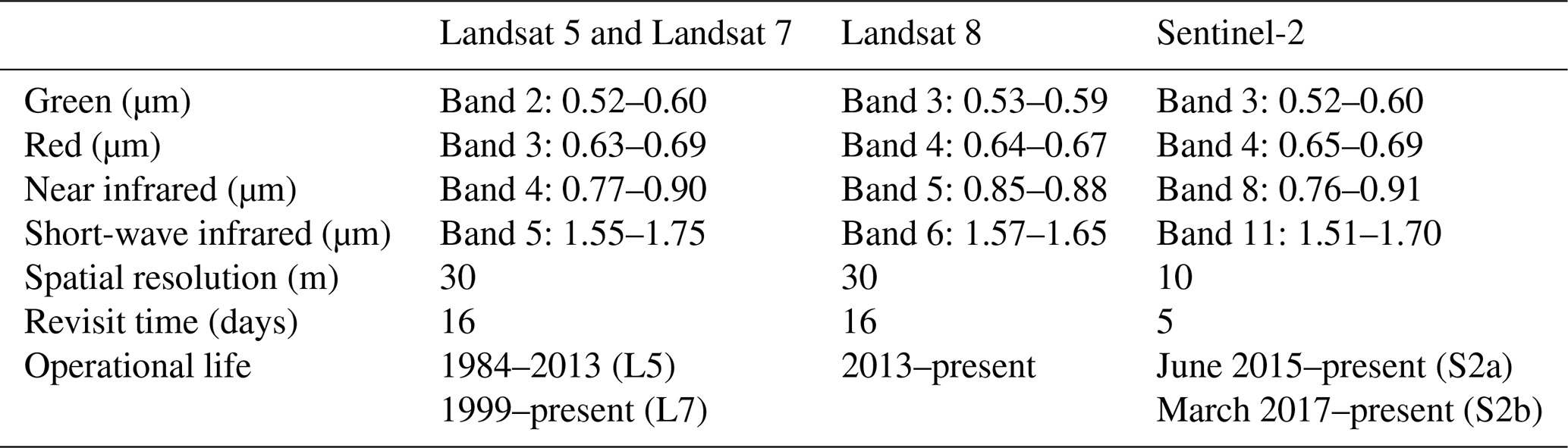
The automated landslide detection index (ALDI) leverages the change in vegetation cover (and the associated spectral signature of reflected light) caused by the removal of vegetation by landslides. The change in spectral signature is typically characterised by a change in the normalised difference vegetation index (NDVI; Tucker, 1979), defined as

$$\begin{array}{}\text{(1)}& \mathrm{NDVI}={\displaystyle \frac{R_{\mathrm{n}}-R_{\mathrm{r}}}{R_{\mathrm{n}}+R_{\mathrm{r}}}},\end{array}$$

where R_n is spectral reflectance in the near-infrared band and R_r is spectral reflectance in the red band (wavelengths in Table 1). The light reflected from landslide-affected pixels, whether they are within the scar or runout area, has a spectral signature associated with rock or sediment. This differs considerably from vegetation in terms of R_n and R_r, resulting in extremely low NDVI values. We call the difference in NDVI before and after the trigger event dV, which is bounded by [−1, 1] and should be negative for landslide pixels associated with the event. This is not in itself a novel approach and is similar to other NDVI differencing approaches (e.g. Behling et al., 2014, 2016; Marc et al., 2019; Scheip and Wegmann, 2021).

Table 1 Landsat and Sentinel image characteristics (Barsi et al., 2014; ESA, 2022).

In addition, vegetation that is disturbed by landslides regrows slowly – over timescales of months to years (Restrepo et al., 2009). Thus, for landslide-affected pixels NDVI should not only reduce after the trigger event but also stay low for an extended period (at least 1 year, depending on climate and seasonality as well as the timing of the earthquake). Therefore, we examine a time series of post-event images to calculate a time-averaged post-event NDVI, which we call V_post, which is bounded by [0, 1] and which should be low for landslide pixels associated with the trigger event.

Averaging over a time series of images has the additional advantage that it enables robust estimates of both dV and V_post even for NDVI time series that are both patchy and noisy. The time series are patchy because cloud cover occludes the ground for some pixels on some days; this cloud can be removed using filtering algorithms (e.g. Irish, 2000; Goodwin et al., 2013), but this leaves a gap in the series. The timing and number of these gaps vary from pixel to pixel, making a comparison of NDVI for particular dates or images problematic. The time series are noisy because atmospheric conditions alter both incoming radiation (e.g. cloud shadow) and that received by the sensor and because ground surface (and especially vegetation) properties will vary over time both periodically (e.g. due to seasonal vegetation growth and harvesting) and randomly (e.g. due to leaf orientation).

Since we expect NDVI to be noisy, we seek a third metric to identify whether there is a shift in NDVI in the presence of broadly consistent seasonal variations and random noise in NDVI. For this we take the difference in NDVI across monthly bins to account for the seasonal component, then quantify the shift in NDVI since the trigger event. For the shift to be indicative of real change it should be considerably larger than the noise present in the NDVI signal. Thus, we express the NDVI shift relative to the noise for each pixel as

$$\begin{array}{}\text{(2)}& t=\sqrt{n}{\displaystyle \frac{\mathrm{d}V}{S_{\mathrm{v}}}},\end{array}$$

where n is the sample size (12 for monthly bins), dV is the mean of the monthly NDVI differences, and S_v is the standard deviation of the monthly NDVI differences. We then normalise this by mapping t onto the cumulative Student's t distribution to generate P_t, the likelihood that the pre- and post-event NDVIs are drawn from different distributions:

$$\begin{array}{}\text{(3)}& P_{\mathrm{t}}=I_{\frac{(n-\mathrm{1})}{n-\mathrm{1}+t^{\mathrm{2}}}}\left({\displaystyle \frac{n-\mathrm{1}}{\mathrm{2}}},{\displaystyle \frac{\mathrm{1}}{\mathrm{2}}}\right),\end{array}$$

where I_x(a,b) is the regularised incomplete beta function. While this is equivalent to a paired t test, the results cannot be interpreted as formal probabilities, as the distribution of dV may not be Gaussian. Rather they represent an index of change relative to expected variability which is bounded by [0, 1]. P_t should be high for landslide pixels associated with the trigger event. High P_t could also result from other events that reduce the coverage or vigour of vegetation, particularly if this involves complete removal (e.g. fire or logging). However, seasonal vegetation changes should be accounted for by examining monthly differences, while episodic events should only be noticeable when (1) their timing is coincident with the earthquake and (2) their effect persists over more than 1 year.

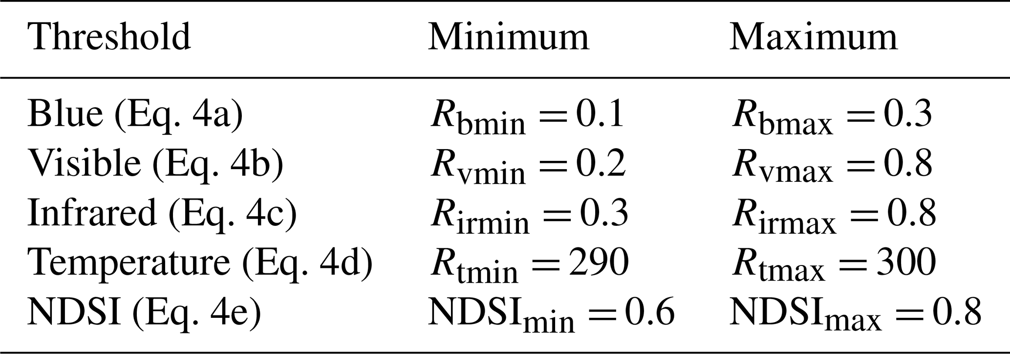
Although low NDVI is effective for identifying the absence of vegetation, it does not uniquely identify landslides, since a range of other surfaces generate similar signatures, particularly snow and cloud. Cloud cover varies from one image to another, and we thus seek to remove cloud-affected pixels from both the pre- and post-event time series. Clouds can be identified based on their spectral signature, with different types resulting in different signatures. The “Landsat simple cloud score” function within Google Earth Engine returns the minimum of a set of five cloudiness indices using Eqs. (4a)–(4f) and parameters in Table 2 (Earth Engine, 2021). Each index reflects an expectation about cloud reflectance and temperature: they should be reasonably bright in the blue band (CI_b), in all visible bands (CI_v), and in all infrared bands (CI_ir); they should be reasonably cool in the thermal infrared band (CI_Temp); but they should not be snow (CI_NDSI):

$$\begin{array}{}\text{(4a)}& {\displaystyle }{\mathrm{CI}}_{\mathrm{b}}={\displaystyle \frac{R_{\mathrm{b}}-R_{\mathrm{bmin}}}{R_{\mathrm{bmax}}-R_{bmin}}},\text{(4b)}& {\displaystyle }{\mathrm{CI}}_{\mathrm{v}}={\displaystyle \frac{\left(R_{\mathrm{r}}+R_{\mathrm{g}}+R_{\mathrm{b}}\right)-R_{\mathrm{vmin}}}{R_{\mathrm{vmax}}-R_{\mathrm{vmin}}}},\text{(4c)}& {\displaystyle }{\mathrm{CI}}_{ir}={\displaystyle \frac{\left(R_{\mathrm{n}}+R_{\mathrm{s}\mathrm{1}}+R_{\mathrm{s}\mathrm{2}}\right)-R_{\mathrm{irmin}}}{R_{\mathrm{irmax}}-R_{\mathrm{irmin}}}},\text{(4d)}& {\displaystyle }{\mathrm{CI}}_{\mathrm{Temp}}=\mathrm{1}-{\displaystyle \frac{R_{\mathrm{t}}-R_{\mathrm{tmin}}}{R_{\mathrm{tmax}}-R_{\mathrm{tmin}}}},\text{(4e)}& {\displaystyle }{\mathrm{CI}}_{\mathrm{NDSI}}=\mathrm{1}-{\displaystyle \frac{\mathrm{NDSI}-{\mathrm{NDSI}}_{\min }}{{\mathrm{NDSI}}_{\max }-{\mathrm{NDSI}}_{\min }}},\text{(4f)}& {\displaystyle }\mathrm{CI}=\min \left({\mathrm{CI}}_{\mathrm{b}},{\mathrm{CI}}_{\mathrm{v}},{\mathrm{CI}}_{\mathrm{ir}},{\mathrm{CI}}_{\mathrm{Temp}},{\mathrm{CI}}_{\mathrm{NDSI}}\right),\end{array}$$

where R_g and R_b are the spectral reflectances from the red and blue bands, R_s1 and R_s2 are those from the first and second short-wave infrared bands, and R_t is that from the thermal infrared band (the only band used here with a coarser 60 m resolution). The parameters with min and max subscripts (e.g. R_bmin and R_bmax for the red band) in Eq. (4) are minimum and maximum values used to normalise pixel reflectances; their values are given in Table 2. NDSI is the normalised difference snow index:

$$\begin{array}{}\text{(5)}& \mathrm{NDSI}={\displaystyle \frac{R_{\mathrm{g}}-R_{\mathrm{s}}}{R_{\mathrm{g}}+R_{\mathrm{s}}}}.\end{array}$$

This index is also used within ALDI outside the Landsat simple cloud score function to identify pixels where persistent snow cover could result in misleading statistics. Where pixels remain snow-covered for periods of several weeks or months, we cannot retain sufficient observations to calculate stable statistics from these pixels. Instead, we identify pixels with persistent snow cover based on time-averaged NDSI and censor them from the analysis.

Table 2 Parameters for Landsat simple cloud score, Eqs. (4a)–(4f).

We define the automated landslide detection index (ALDI) as the product of the three parameters defined above. While this formulation is entirely arbitrary, it has the advantage of allowing the index to take a minimum value of zero (indicating negligible probability that the images reflect a landslide at that location) if any of the individual terms is zero. Because we have no a priori knowledge of the relative importance of each parameter in determining the landslide signature, we assume a power-functional form with empirical exponents α, β, and λ:

$$\begin{array}{}\text{(6)}& \mathrm{ALDI}=\left\{\begin{array}{l}{\left(-\mathrm{d}V\right)}^{\mathit{\alpha }}{\left(\mathrm{1}-V_{\mathrm{post}}\right)}^{\mathit{\beta }}{P}_{\mathrm{t}}^{\mathit{\lambda }},\\ \mathrm{0},\end{array}\right.\begin{array}{l}\mathrm{if}{S}_{\mathrm{post}}>T_{\mathrm{snow}}\mathrm{|}\mathrm{d}V<\mathrm{0}\\ \mathrm{otherwise}\end{array},\end{array}$$

where S_post is the mean post-earthquake NDSI and T_snow is a threshold value for NDSI, chosen to identify persistent snow cover. The likelihood that a pixel is landslide-affected increases monotonically with the ALDI output value, which has upper and lower bounds of 0 and 1, respectively. Landslide pixels should be characterised by negative dV, indicating vegetation removal; low V_post, indicating a lack of vegetation after the earthquake; and high P_t, due to a distinguishable shift in post-event NDVI distributions relative to the pre-event distributions. The likelihood that a pixel contains a landslide should increase with P_t and decrease with dV and V_post. We exclude snow-dominated pixels where S_post exceeds threshold T_snow, as well as pixels where median post-earthquake exceeds pre-earthquake NDVI (i.e. positive dV).

The empirical exponents α, β, and λ can be expressed in terms of one parameter (α) and two ratios (α : β and α : λ) because

$$\begin{array}{}\text{(7)}& \mathit{\beta }=\mathit{\alpha }{\displaystyle \frac{\mathrm{1}}{\mathit{\alpha }:\mathit{\beta }}}\mathrm{and}\mathit{\lambda }=\mathit{\alpha }{\displaystyle \frac{\mathrm{1}}{\mathit{\alpha }:\mathit{\lambda }}},\end{array}$$

substituting the following terms into Eq. (6),

$$\begin{array}{}\text{(8)}& \mathrm{ALDI}=\left\{\begin{array}{l}{\left(-\mathrm{d}V\right)}^{\mathit{\alpha }}{\left(\mathrm{1}-V_{\mathrm{post}}\right)}^{\mathit{\alpha }\frac{\mathrm{1}}{\mathit{\alpha }:\mathit{\beta }}}{P}_{\mathrm{t}}^{\mathit{\alpha }\frac{\mathrm{1}}{\mathit{\alpha }:\mathit{\lambda }}},\\ \mathrm{0},\end{array}\right.\begin{array}{l}\mathrm{if}{S}_{\mathrm{post}}>T_{\mathrm{snow}}\mathrm{|}\mathrm{d}V<\mathrm{0}\\ \mathrm{otherwise}\end{array},\end{array}$$

then taking logarithms of both sides clarifies the role of the ratio parameters. This yields

$$\begin{array}{}\text{(9)}& \begin{array}{rl}\log \left(\mathrm{ALDI}\right)& =\mathit{\alpha }(\log \left(-\mathrm{d}V\right)+{\displaystyle \frac{\mathrm{1}}{\mathit{\alpha }:\mathit{\beta }}}\log \left(\mathrm{1}-V_{\mathrm{post}}\right)\\ & +{\displaystyle \frac{\mathrm{1}}{\mathit{\alpha }:\mathit{\lambda }}}\log \left(P_{\mathrm{t}}\right)).\end{array}\end{array}$$

The values of dV, V_post, and P_t are all ≤ 1 (thus their logarithms are negative), and larger values of the ratio parameters (α : β and α : λ) result in smaller powers for their respective layers (V_post and P_t). Therefore, large α : β ratios result in a stronger influence of V_post on ALDI; large α : λ ratios result in the same for P_t; and when both α : β and α : λ are small, dV dominates. These ratios are more informative than the raw parameters because it is the relationship between exponents rather than the exponents themselves which defines the relative role of the different ALDI components (i.e. equal but high values of α, β, and λ result in the same ALDI classification pattern as equal but low values).

3.2 ALDI classifier implementation and data pre-processing

We implement ALDI and perform all pre-processing steps within Google Earth Engine (GEE; Gorelick et al., 2017) because (1) it hosts an extensive Landsat archive and provides efficient access to large volumes of freely available satellite data; (2) it provides both a toolkit of pre-compiled algorithms for image processing and cloud computing resources to run these algorithms; and (3) it is an open-access platform so that both the data and the algorithms used here are widely accessible and reproducible (see Milledge, 2021, for source code).

The objective of pre-processing is to generate four layers: dV, the change in NDVI before and after the trigger event; V_post, the time-averaged post-event NDVI; S_post, the post-event NDSI; and P_t, the likelihood that pre- and post-event NDVIs are drawn from different distributions. These layers should synthesise the time series of available imagery from multiple sensors minimising bias due to the sensor, the influence of clouds, and seasonal vegetation changes.

We use time series of NDVI calculated from Landsat 5, Landsat 7, and Landsat 8 imagery following “top-of-atmosphere” correction (Chander et al., 2009) to adjust for radiometric variations due to solar illumination geometry (angle and distance to Sun) and sensor-specific gains and offsets. Sentinel-2 data would offer additional gains in terms of both spatial and temporal resolution of data but are not available for any of our case study events and thus cannot yet be evaluated within the same framework. Landsat 8 sensors aggregate red and near-infrared reflectance over slightly different frequency bands to Landsat 5 and Landsat 7, but their central frequencies vary by < 4 % between sensors and by > 20 % between bands (Table 1). To ensure satisfactory image-to-image registration for time series analysis, we use only images which have been both georeferenced to ground control points and terrain-corrected (i.e. Level 1TP) and thus have ≤ 12 m radial root mean square error (RMSE) in > 90 % of cases (USGS, 2019).

The time series is split into two “stacks” of images, those before the trigger event and those after it (Fig. 1b). The duration of these time series (and thus length of stacks) reflects a trade-off between shorter durations, which limit the sample size, and longer durations, which include landscape changes unrelated to the earthquake. We remove “cloudy” pixels from each stack using the GEE simple cloud score exceeding a tuneable threshold (T_cloud), where stricter thresholds not only remove more cloudy pixels but also incorrectly remove more cloud-free false positives (Earth Engine, 2018). The number of images in each stack is controlled by the stack lengths and cloud threshold, introducing three tuneable parameters to be calibrated. These parameters are found using the calibration process described in Sect. 3.4 rather than by considering the physical processes that characterise the possible evolution of the time series.

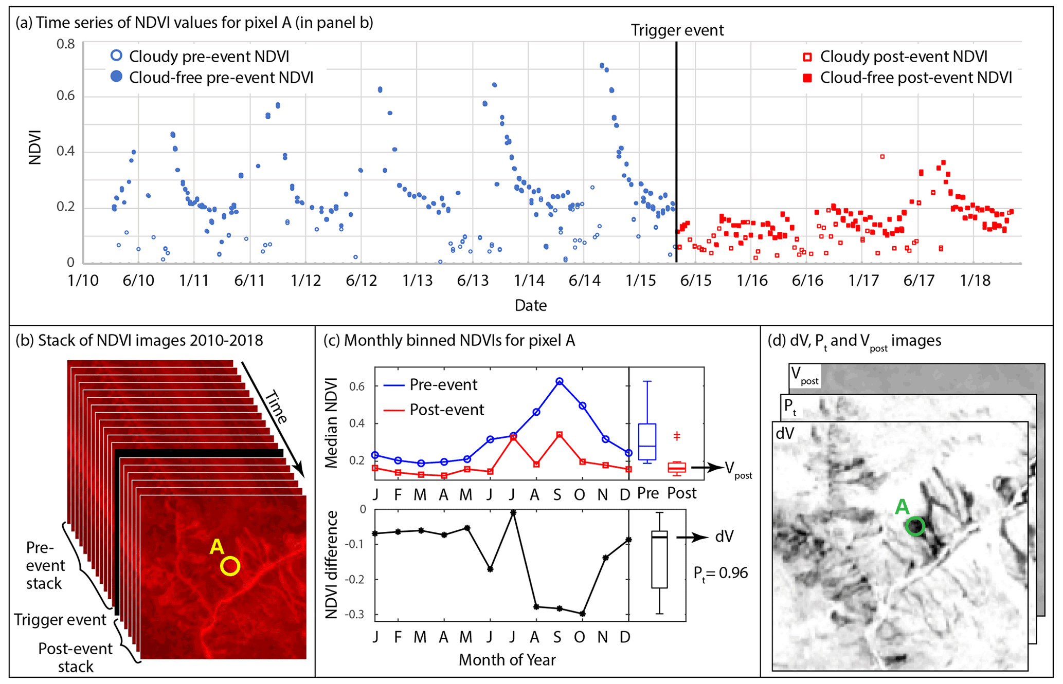
Figure 1 ALDI pre-processing steps. (a) Time series of NDVI values for a single landslide-affected pixel (circled in panels b and d) before and after the trigger event, with cloud-free values shown as solid symbols. This time series is derived from a stack of NDVI images (b) and is used to calculate monthly median NDVI before and after the earthquake and their difference (c), which can be used to calculate dV, P_t, and V_post for every pixel in the study area (d). Please note that the date format in this figure is month/year.

To account for seasonal vegetation change, NDVI values for each pixel in the pre- and post-earthquake stacks are extracted as a time series (Fig. 1a) and binned based on the month in which the image was acquired. Monthly bins are used since they are generally long enough to contain data in every bin (even after removal of cloudy pixels) but short enough to capture annual seasonality (e.g. Fig. 1a). Monthly bins result in four images per bin per year on average, and thus empty bins are very unlikely except for month–location pairs that are characterised by extreme cloudiness (such as Nepal in July; see Wilson and Jetz, 2016). Monthly bins that are empty in either the pre- or post-earthquake period are not used in the subsequent analysis, with calculations for that pixel performed using the remaining monthly bins. We calculate median NDVI for each monthly bin, choosing median rather than mean, since it is less sensitive to skew and to extreme values (Fig. 1c). We difference the monthly median values prior to and after the trigger event, generating a distribution of differences (Fig. 1c). From that distribution, we calculate the mean monthly NDVI difference (dV) and evaluate the likelihood that the mean monthly NDVI difference differs significantly from zero using a pairwise t test to calculate P_t. We take the mean of the post-event monthly NDVI values to generate V_post, then apply a similar procedure to the pixel-wise NDSI values to calculate the mean of the post-event monthly NDSI, S_post. This allows us to construct maps of the pixel-wise values of dV, V_post, S_post, and P_t (Fig. 1d) and thus to evaluate Eq. (6). The full routine runs in GEE in less than 30 min for an area of ∼ 10⁴ km² (ca. 10⁷ pixels).

3.3 Performance testing

We evaluate ALDI performance in terms of its ability to reproduce the location and size of manually mapped landslides. For each earthquake inventory we define a study area based either on the area defined by the manual mappers (e.g. excluding areas where cloud or snow cover hampered manual mapping) or, where this is not available, on a convex hull that bounds the landslide inventory.

ALDI returns a continuous relative measure of the certainty with which a pixel is classified as a landslide. To evaluate this measure against a manually mapped landslide inventory it must be converted into a binary classification by thresholding the classification surface. The manual map is then rasterised to the same resolution as the classification surface – in this case, 30 m – using a “majority area” rule, whereby landslide pixels are those with the majority of their area overlapped by landslide polygons. The benefit of a given classification can then be quantified in terms of success in identifying positive (landslide) and negative (non-landslide) outcomes on a pixel-by-pixel basis. Thresholding the classification surface is a difficult exercise involving a trade-off between sensitivity, the fraction of the landslides that should be captured (also known as the true-positive rate, TPR – the number of true positives normalised by all positive observations), and specificity, the number of false positives that should be allowed in doing so (also known as the false-positive rate, FPR – the number of false positives normalised by all negative observations). In practice, this threshold is often set by external requirements in terms of a desired sensitivity or specificity, but these requirements can vary considerably between users and applications.

Receiver operating characteristic (ROC) curves provide a more complete quantification of the performance of the classifier (e.g. Frattini et al., 2010). The ROC curve is constructed by incrementally thresholding the classifier and evaluating true- and false-positive rates at different threshold values to generate a curve where the 1 : 1 line reflects the naïve (i.e. random) case. The true- and false-positive rates are insensitive to imbalanced data and thus are well suited to the evaluation of landslide classification, which typically has many more non-landslide than landslide pixels (García et al., 2010). The area under the curve (AUC) tends to 1 as the skill of the classifier improves towards perfect classification and to 0.5 as the classifier worsens towards the naïve (random) case. The strength of AUC is that it avoids the need to threshold the classifier and is widely used, enabling comparison with other landslide detection methods; its main weakness is that it is difficult to interpret in absolute terms. What AUC value constitutes “good” performance?

In our case, we seek to establish whether automated detection performance is such that it can be used as an alternative to manual mapping. However, it is difficult to compare the ALDI output against manual mapping because manual mapping is itself being used as the ground truth in the absence of a better alternative. To address this, we first test the agreement between manual inventories in terms of true- and false-positive rates. TPR_I1-2 indicates the fraction of landslides in inventory I1 that are also predicted by I2, and FPR_I1-2 indicates the fraction of non-landslide pixels in I1 that are “incorrectly” identified as landslide pixels by I2.

ALDI performance in identifying landslide location on a pixel-by-pixel basis can then be compared against one of the manual maps as a competitor with the other manual map used as the check dataset. To enable the comparison, we first threshold the ALDI output to generate a binary classifier with the same FPR as the competitor inventory with respect to the check inventory. The ability of ALDI to successfully identify more landslide pixels than the competitor inventory can then be calculated from the difference in their true-positive rates as TPR_diff:

$$\begin{array}{}\text{(10)}& {\mathrm{TPR}}_{\mathrm{diff}}={\mathrm{TPR}}_{\mathrm{ALDI}}-{\mathrm{TPR}}_{\mathrm{Comp}},{\mathrm{FPR}}_{\mathrm{ALDI}}={\mathrm{FPR}}_{\mathrm{Comp}},\end{array}$$

where TPR_ALDI and FPR_ALDI are the ALDI true- and false-positive rates, respectively, both calculated from the check inventory, and TPR_Comp and FPR_Comp are the true- and false-positive rates for the competitor inventory, also calculated from the check inventory. The magnitude of TPR_diff indicates the similarity in performance, while the sign indicates the best performer (positive values indicate that ALDI outperforms manual mapping and vice versa). This approach allows for direct comparison between ALDI and manual mapping for the same classification threshold. Other metrics could be derived from the confusion matrix (e.g. Tharwat, 2020; Prakash et al., 2020), but these typically require assumptions about the relative weight assigned to true and false positives and negatives. Our approach avoids these assumptions because the ALDI output is thresholded to ensure that FPRs are equal to those of the competitor inventory.

In addition, we express spatial mapping error between manual inventories as the ratio of the intersection of the two maps to their union. This is equivalent to the “degree of matching” (Carrara et al., 1992; Galli et al., 2008) and can be interpreted as the percentage of total mapped landslide area that the inventories have in common.

To examine the ability of ALDI to recover landslide size information we compare the area–frequency distributions of landslides from each manual map with those for landslides detected by ALDI. For manually mapped inventories this information is generally captured automatically, since landslides are mapped as discrete objects rather than on a pixel-by-pixel basis. However, automated classifiers like ALDI require additional steps to convert a continuous pixel-based classification surface to a set of landslide objects. First, we generate a binary prediction of landslide presence or absence by thresholding the ALDI classification surface to match the manually mapped FPR, as described above. The manual inventories examined here typically have very low FPRs (< 2 % of TPR on average and < 7 % at most, Table 3). Second, we convert the binary landslide map to a set of landslide objects by identifying connected components at the 30 m resolution of the Landsat imagery (Haralick and Shapiro, 1992). This connected-component clustering is one of the simplest of many possible clustering algorithms. Finally, we calculate the area of individual landslide objects from the number of pixels in each object (cluster) and generate an area–frequency distribution.

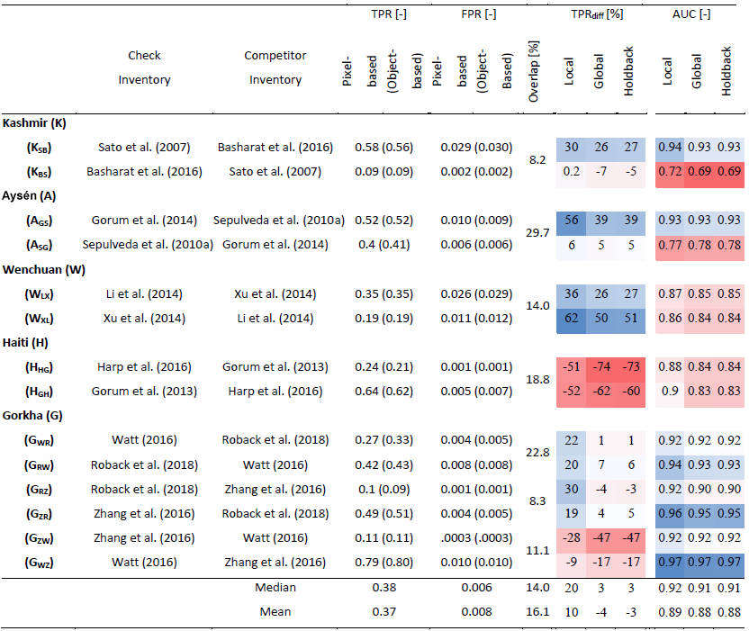
Table 3 Performance metrics for ALDI applied with the different parameter sets to identify landslide-affected areas from each of the 14 inventory pairs. Abbreviated names for the inventory pairs indicate the case study with subscripts denoting first check and then competitor inventories (e.g. K_SB denotes the Kashmir earthquake with Sato as the check inventory and Basharat as the competitor inventory). The true-positive rate (TPR) and false-positive rate (FPR) are reported for both object-based analysis (in brackets) and pixel-based analysis at 30 m resolution. Overlap indicates the percentage overlap between pairs of landslide inventories. Shading in right-hand columns indicates performance of ALDI relative to each competitor and for each metric and calibration, with a linear colour scale from blue where ALDI outperforms the manual competitor to red where the manual competitor outperforms ALDI. Vertical blocks reflect different performance metrics: TPR_diff and AUC (see text). Columns within each block reflect different ALDI calibration strategies: local calibration optimised to both site and check inventory, global calibration using a compilation of the best parameter sets from all sites, and holdback calibration where parameter sets from the test site are excluded. Note that positive values of TPR_diff reflect cases where ALDI outperforms manual mapping, while negative values reflect cases where manual mapping is better.

3.4 Parameter calibration and uncertainty estimation

The ALDI landslide classifier has seven tuneable parameters: cloud threshold (T_cloud), pre-event stack length (L_pre), post-event stack length (L_post), snow threshold (T_snow), and the three exponents (α, β, and λ) that control the weighting assigned to the V_post, dV, and P_t layers, respectively. Calibrating the parameters and estimating the associated uncertainty is important because the parameters are difficult or impossible to set a priori and because we seek to develop a general model that can be applied to new landslide events not examined here. Our calibration seeks to optimise classifier performance evaluated by comparing the classifier to 11 manually mapped landslide inventories using the performance metrics described in Sect. 3.3.

We calibrate ALDI parameters using one-at-a-time calibration for parameters that are internal to the GEE routine (T_cloud, L_pre, L_post), since these parameters are well constrained (in the case of T_cloud and L_post) or have a limited number of possible values (in the case of L_pre and L_post). We use an informal Bayesian calibration procedure (e.g. Beven and Binley, 1992) for parameters in Eq. (6) (T_snow α, β, and λ), since these parameters are less well constrained, but evaluation of Eq. (6) is computationally cheap. We calibrate L_post, L_pre, and T_cloud one-at-a-time (in that order) for each earthquake event then test alternative near-optimum parameter combinations to minimise the effect of the calibration order. These combinations are obtained by varying L_post by ± 1 year for optimum values of L_pre and T_cloud and doing the same for L_pre at optimum values of L_post and T_cloud. For each GEE run in the one-at-a-time process we run 500 simulations of Eq. (6) with T_snow and α randomly sampled from uniform probability distributions and the ratio parameters sampled from uniform distributions of log₁₀(α : β) and log₁₀(α : λ). We sample the ratio parameters in logarithmic space to maintain symmetric sampling density with distance from a ratio of unity (e.g. α : β= 0.1, where β= 10α should be sampled as densely as α : β=10, where α= 10β).

We examine L_post of up to 5 years because vegetation typically begins to regrow over this timescale (Restrepo et al., 2009) and L_pre of up to 10 years because we expect that other landscape changes (e.g. fire, drought, and landslides caused by other triggers) will begin to disrupt the pre-event signal at longer timescales. In both cases we examine only integer year values to ensure consistent sampling within the monthly bins. We use the full range of NDSI values for T_snow ([0, 1]) and cloud score values for T_cloud ([0, 1]). For the three exponents, we use zero for the lower bound and iteratively refine the upper bound to ensure that optimum performance at any site is found to be within the range.

We perform the calibration for individual earthquakes to estimate the optimum classification skill that could be obtained when calibrating on all the check data. We then retain the best 20 parameter sets (measured in terms of AUC) from each earthquake to generate a global set of 100 parameter sets. To account for parameter interaction (particularly between the three exponents α, β, and λ) within a set we retain parameter sets as seven-element vectors. To ensure that each manually mapped landslide inventory is given equal weight as a check dataset we calibrate to each in turn taking 7 parameter sets from calibration to each of the 3 Gorkha inventories and 10 from each of the 2 inventories at the other sites. Finally, we run ALDI with each of these 100 parameter sets to generate 100 ALDI classification surfaces then take the mean for each cell.

To simulate the “blind” application of ALDI to future events, we perform a holdback test in which we run ALDI using the global-parameter set but hold back the 20 parameter sets that were derived from the site at which testing is being performed. In this test the parameters used to run ALDI are uninfluenced by the specific behaviour of the test site.

4 Results

4.1 Spatial agreement: Gorkha case study

We first illustrate our approach using the 2015 Gorkha earthquake, where three manual inventories are available, and then consider the other four earthquakes introduced in Sect. 2. All three manual inventories for the Gorkha earthquake show an elongated cluster of landslides extending from northwest to southeast (Fig. 2a) that coincides with the area of steep slopes that experienced the most intense shaking. However, when the maps are compared at a finer scale they differ considerably (Fig. 2c, e). In some cases, one mapper has identified a landslide, but one or both of the others have not (e.g. location A in Fig. 2e). Some, but not all, of these missed landslides can be attributed to areas where imagery was unavailable or where the ground was obscured by clouds (shown as grey areas in Fig. 2c). In other cases, mapped landslides overlap, but their size and/or shape differ, due either to differences in the interpretation of landslide boundaries (e.g. location B in Fig. 2e) or to the georeferencing of the underlying imagery from which the landslides were mapped. Georeferencing differences seem particularly likely to explain mapped landslides of very similar size and shape that are offset by small distances (e.g. location C in Fig. 2e) or appear distorted relative to one another so that their outlines only partially overlap (e.g. location D in Fig. 2e).

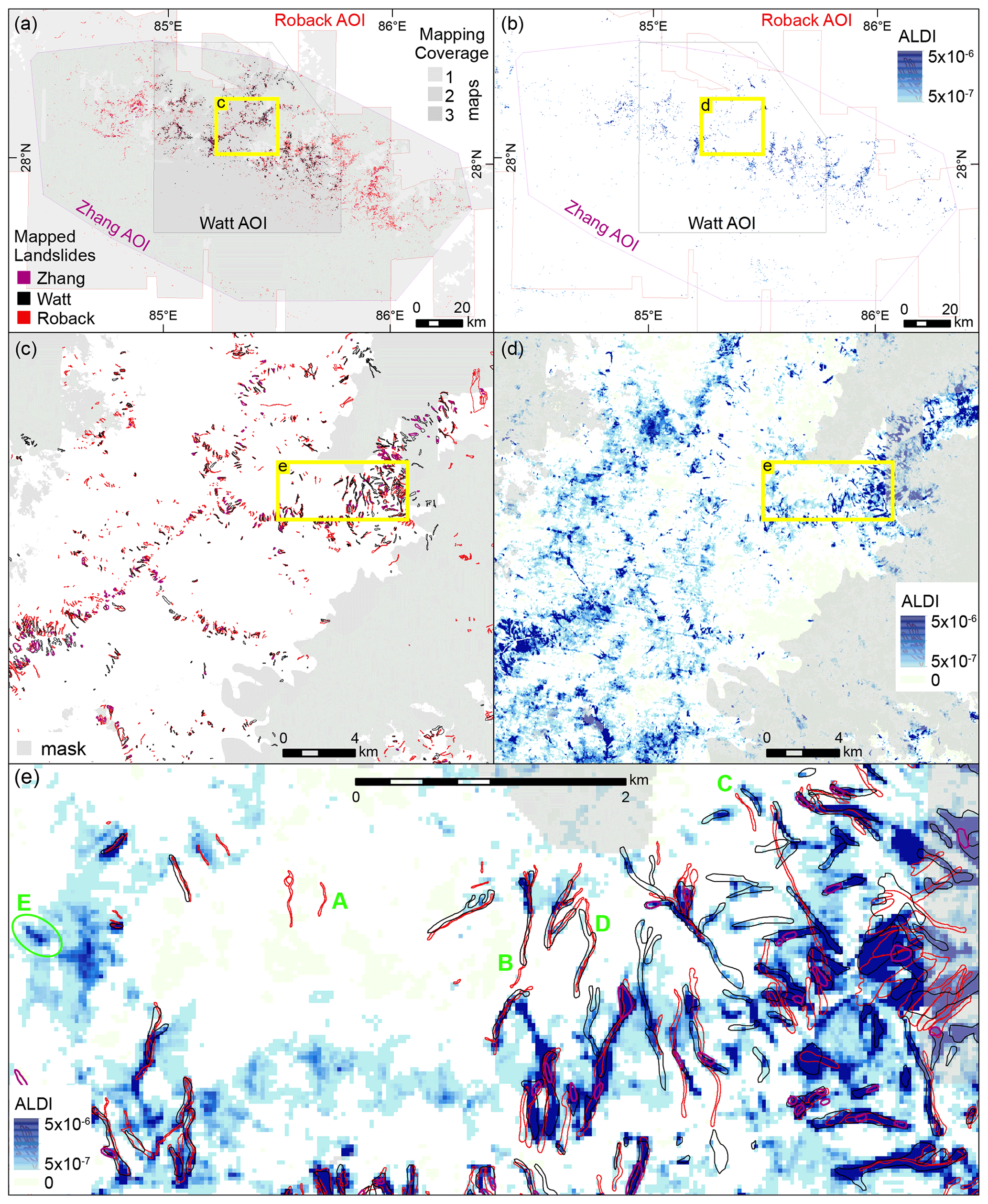
Figure 2 Mapped landslides and the ALDI classifier for the Gorkha study site. (a) Mapped landslides at the scale of the full study area with AOIs (areas of interest; the mapped area) shown in grey. Zhang, Roback, and Watt refer to the inventories of Zhang et al. (2016), Roback et al. (2018), and Watt (2016). (b) ALDI values for the full study area, using locally optimised parameters. (c) Mapped landslides from the three inventories for a subset of the study area, with areas that were unmapped in one or more inventory shaded grey. (d) ALDI values using locally optimised parameters for the same subset of the study area shown in (c). (e) Detailed view of mapped landslides from the three inventories and ALDI values. Yellow boxes in each panel show the locations of nested panels (e.g. c in a and d in b). Green labels in (e) indicate examples of (A) missed landslides, (B) agreement between inventories, (C) offset landslide outlines, (D) distorted landslide outlines, and (F) landslides identified by ALDI but missed by manual mapping.

The ALDI classifier applied to the Gorkha earthquake captures the broad spatial pattern of mapped co-seismic landslides with large patches of high ALDI values, and thus high classification likelihood, corresponding to clusters of mapped landslides (Fig. 2b). Examining a subsection of the study area (Fig. 2d) shows that ALDI identifies the same broad zones of more intense landsliding as identified in the manual mapping. However, the ALDI output also contains a series of stripes ∼ 1 km apart and ∼ 150 m wide trending west-northwest to east-southeast most clearly visible across the centre of the map. These are the result of data gaps in Landsat 7 images since 2003 due to Scan Line Corrector (SLC) failure on the Landsat 7 sensor. Although both pre- and post-event image stacks include Landsat 5 and Landsat 8 images in addition to Landsat 7, these data gaps clearly influence the ALDI output, with high values more likely for pixels where Landsat 7 data are not available.

Zooming in to a smaller subsection of the study area suggests that most of the landslides that are included in both inventories overlap areas of high ALDI values (Fig. 2e). In addition, areas of high ALDI values overlap many of those landslides identified by one inventory but not the other, although there are mapped landslides that do not overlap areas with high ALDI values (Fig. 2e). In many cases, the patches of high ALDI values have shapes that closely follow those of the mapped landslides (Fig. 2e). In other cases, patches of high ALDI values have typical landslide morphology but are not in either inventory (e.g. location E in Fig. 2e), raising the question of whether these should be considered genuine classifier false positives or are in fact landslides missed in all three manual maps. Given that each inventory misses landslides identified by another, this possibility cannot be excluded. In other cases, the patches of high ALDI values have a size and/or shape that suggest that they are misclassifications. These may be due to clouds, shadows, snow, or other landscape changes not associated with landslides (e.g. crop harvesting, river channel change, building construction).

4.2 ALDI calibration: Gorkha case study

In this section, we seek to establish the best possible ALDI performance when parameters can be optimised to a single study site and identify the influence of parameters on that performance, both in terms of sensitivity to the parameter and preferred range for the parameter. We illustrate this using the Gorkha earthquake, calibrating ALDI's seven tuneable parameters (columns a–g in Fig. 3) to optimise agreement with two of the manually mapped landslide inventories measured using our two performance metrics (rows in Fig. 3). The results are visualised in Fig. 3 using dotty plots (after Beven and Binley, 1992): a matrix of scatter plots where each subplot shows model performance (y axis) against a parameter value (x axis). The histogram above each scatter plot shows the frequency distribution of parameter values for the best 50 model runs for that metric and check dataset.

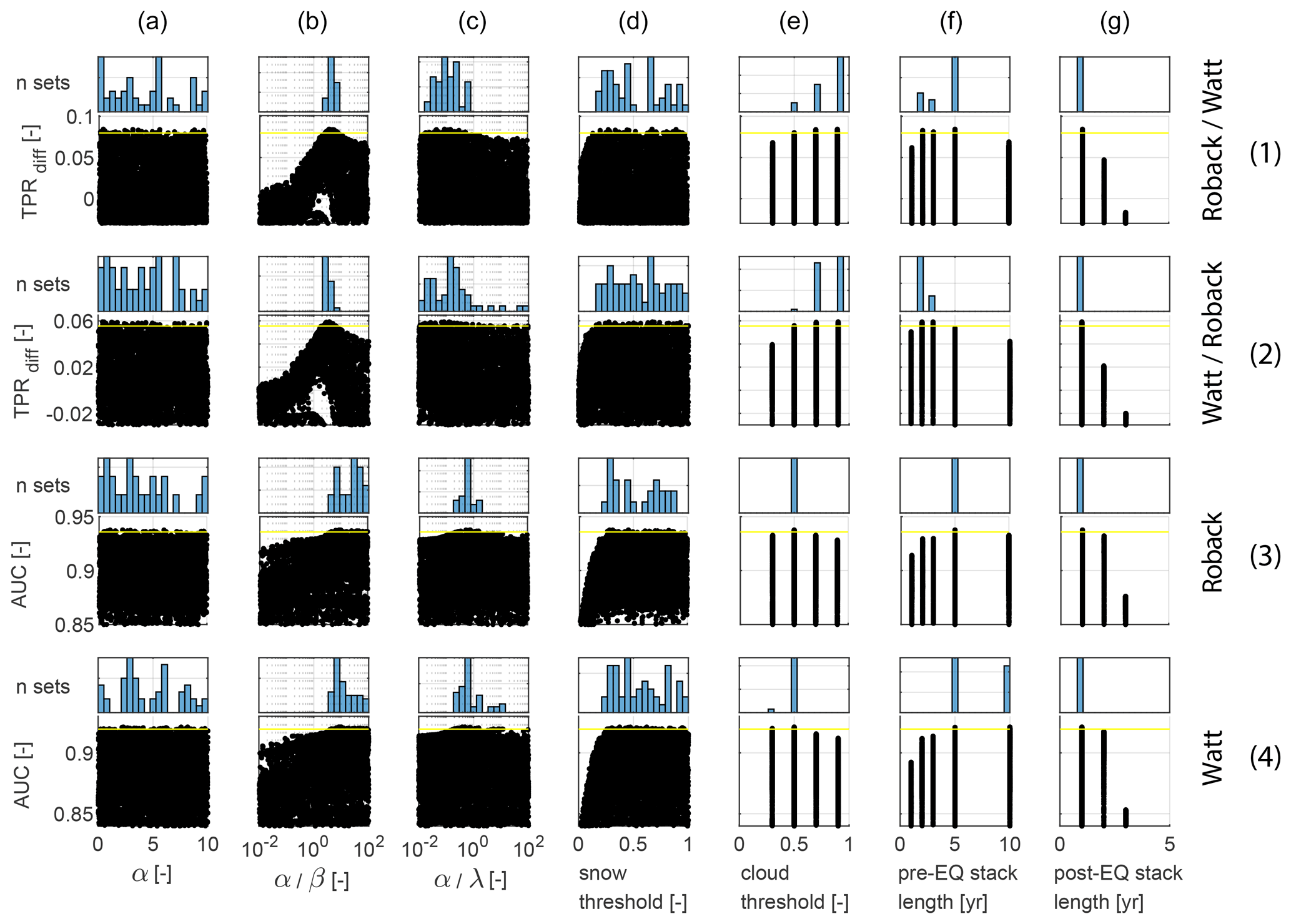
Figure 3 Dotty plots and posterior parameter distributions for the Gorkha case study for the seven tuneable parameters associated with ALDI (columns) evaluated using two of the test datasets (Watt and Roback) and two performance metrics (rows): (1) TPR_diff, the difference in TPR between ALDI and the competitor inventory at the FPR defined by the competitor inventory, and (2) AUC, the area under the ROC curve, a more general indicator of classifier performance over the full range of FPRs. “Roback/Watt” refers to using Roback as the check dataset and Watt as the competitor in row 1; “Watt/Roback” refers to the converse in row 2. Roback is used as the check dataset in row 3, and Watt is the check dataset in row 4. Points plotting above the yellow line are results for the best 100 parameter values. In each case the parameter distributions are for the best 100 parameter sets evaluated using the same metric and datasets as the dotty plot below it. Dotty plots for the other Gorkha inventories and for all other sites are given in the Supplement. EQ: earthquake.

All the scatter plots in Fig. 3 show wide scatter in performance for a single value of any given parameter, indicating that the model is sensitive to multiple parameters. However, the key feature of each plot is the upper bound on ALDI performance for a given parameter value and the sensitivity of this upper bound to change in that parameter. This upper bound can be interpreted as the best possible ALDI performance at value x of parameter A when all other parameters are given flexibility to optimise. Plots where this upper bound is near horizontal suggest limited influence of a particular parameter and are accompanied by broad histograms. Narrow peaks in a plot's upper bound indicate that good model performance requires that parameter to be set within a narrow range, with performance degrading rapidly as values depart from this range independent of other parameter values. In the following paragraphs we examine the influence of each parameter in turn (Fig. 3).

Setting the pre- and post-earthquake stack lengths (L_pre and L_post, respectively) involves a trade-off between errors caused by landslides (or other landscape changes) not associated with the earthquake, if the stack is too long, and errors caused by cloud cover, if the stack is too short. For the Gorkha earthquake, ALDI performance is most sensitive to L_post, indicated by the steep gradient in upper-bound performance across both metrics and for all check datasets (Fig. 3, column g). For all metrics and datasets, a post-earthquake stack length of only 1 year produces the best performance. This may be because longer stacks are more likely to include other landscape changes after the earthquake that disrupt the signal, such as post-seismic landslides or re-vegetation of co-seismic landslides.

ALDI allows landslides to be identified only in pixels where NDSI is lower than the snow threshold (T_snow). ALDI performs well (i.e. < 20 % from optimum) for T_snow values ranging from 0.1 to 0.9 (Fig. 4, column d). For TPR_diff the best values of T_snow are 0.2–0.4 with a rapid decline in performance as T_snow is reduced and a slow decline as it is increased (Fig. 4, rows 1–2 of column d). This suggests that snow rarely causes false positives even when little effort is made to remove it but that an overly conservative snow threshold results in landslides being misclassified as snow. The AUC metric behaves similarly to TPR_diff with a larger performance reduction at low T_snow values and reduced performance reduction at high T_snow values (Fig. 4, rows 3–4 of column d).

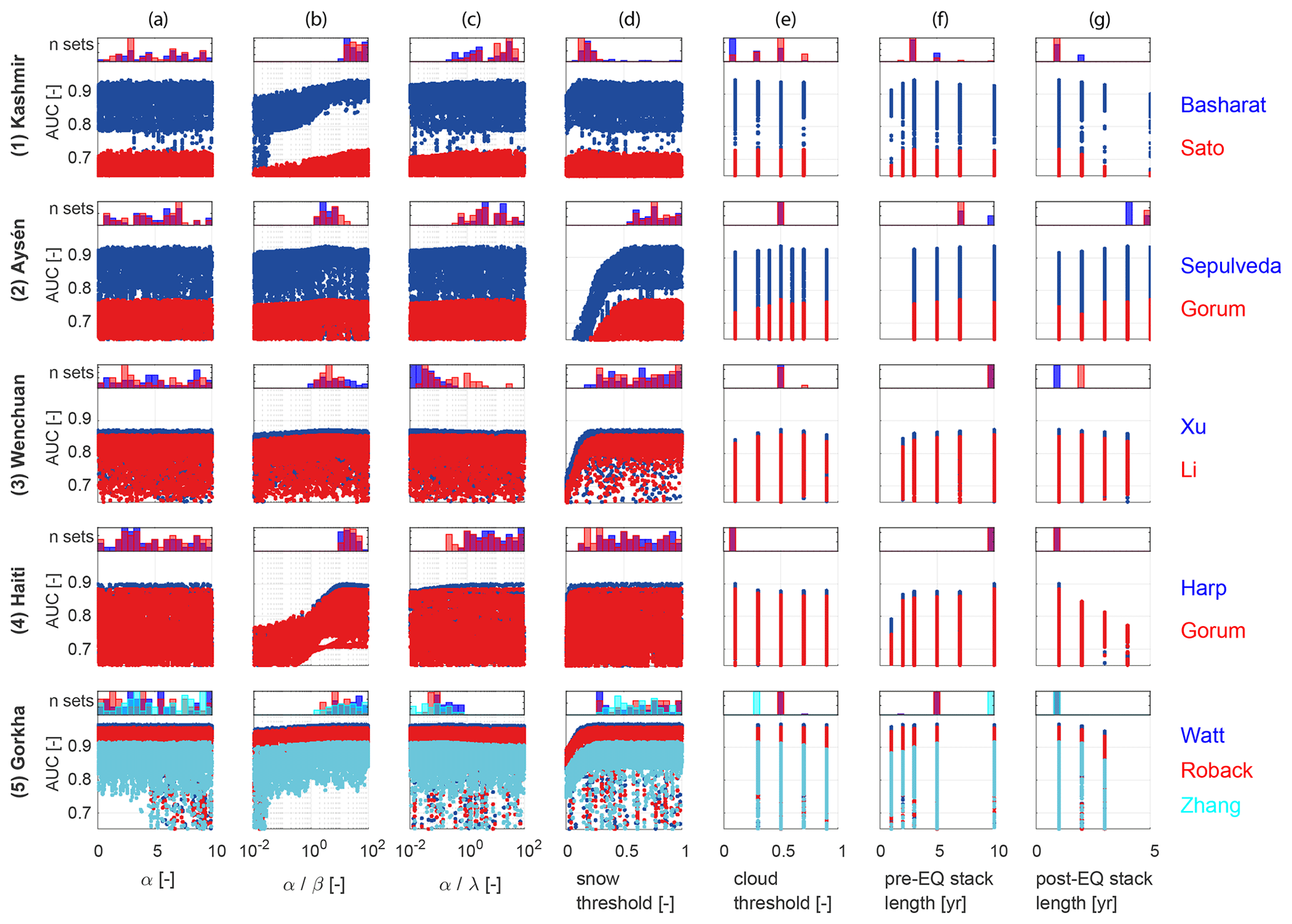
Figure 4 Dotty plots and posterior parameter distributions for the seven tuneable parameters associated with ALDI (columns a–g) for the five study earthquakes (rows 1–5). Dotty plots show classifier performance evaluated using AUC, the area under the ROC curve. Blue or red colours indicate the inventory used as the check dataset, as shown to the right. Parameter distributions are for the best 100 parameter sets evaluated using the same metric. EQ: earthquake.

The α : β ratio controls the influence of change in NDVI (dV) relative to mean post-earthquake NDVI (V_post). Noting that dV and V_post are bounded to be < 1 and that by definition β=α(α : β)⁻¹, larger values of α : β result in smaller exponents on V_post and larger values of the term. ALDI is thus dominated by V_post at higher α : β ratios and by dV at lower ratios. There is a clear optimum within the parameter space and a large reduction in performance away from this optimum indicating that both layers (dV and V_post) are important components of the classifier (Fig. 3, column b). Best performances are found in the range α : β = 3–4 for TPR_diff and in the range α : β= 10–20 for AUC, suggesting that more weight needs to be given to V_post to successfully identify landslides, particularly when bulk performance over the full ROC curve is of primary concern.

The α : λ ratio controls the influence of change in NDVI (dV) relative to the likelihood that the dV values in the post-event stack are significantly different from those in the pre-event stack (P_t). As explained above, ALDI is dominated by P_t at higher α : λ ratios and by dV at lower ratios. ALDI performance is somewhat sensitive to this parameter for both TPR_diff and AUC, with gentle but consistent slopes to the upper-bound performances (Fig. 3, column c). Best performances are found for α : λ in the range 0.01–1 for TPR_diff and 0.1–5 for AUC, suggesting that, although both layers contribute important information, dV is a stronger predictor than P_t for the Gorkha case study.

Optimum parameters for the Gorkha study site differ slightly between performance metrics (compare histograms down columns in Fig. 3). This reflects the different focus of the metrics, where TPR_diff gives the strongest weight to very conservative (i.e. low FPR) classification thresholds (Fig. 3, rows 1–2), and AUC weights all classification thresholds equally (Fig. 3, rows 3–4). In general, the parameters to which ALDI performance is most sensitive are also those for which optimum values are most robust to changes in check dataset or performance metric. For example, there is negligible change in optimum values for L_post and T_snow across the range of metrics and datasets. α : β and α : λ are both broadly comparable between metrics, although in both cases there is a shift towards higher optimum values for AUC, indicating that for this metric NDVI difference is less important than it was for TPR_diff (noting that the improvement is always < 3%). α : β has a progressively less clear optimum as metrics become more generalised (from TPR_diff to AUC) indicating reduced parameter sensitivity for AUC. T_cloud and L_pre have larger changes in optimised parameters between the metrics, although the sensitivity to these changes is small in performance terms (Fig. 3, columns e–f). Optimum T_cloud is 0.7 for TPR_diff but 0.5 for AUC; optimum L_pre is in the range 2–5 for TPR_diff and 5–10 for AUC. ALDI performance is insensitive to α, varying by < 10 % across the parameter range for all metrics, generating a broad histogram of best-performing parameter values and showing large shifts in the optimum value depending on both the metric and the dataset used to assess performance (Fig. 3, column a).

4.3 ALDI calibration: global comparison

We focus our global comparison on the AUC performance metric. Results for TPR_diff are very similar and can be found in the Supplement (Figs. S1–S6). Figure 4 shows that optimum values for a given parameter differ between sites; that sensitive parameters at one site are usually sensitive at others; and that absolute performance differences between different inventories at a site can be large, although the trends are generally similar.

ALDI is sensitive to L_post for all sites but with trends that differ between sites: for Haiti and Gorkha a value of 1 year is best, 2 years is reasonable, and 3 years is poor. For Kashmir and Wenchuan a value of 1 year is best, but a value of 2 years also gives reasonable results. For Aysén a value of 5 years is best, and a value of 1 year is particularly poor (Fig. 4, column g). An L_post of 2 years generally results in fairly good performances for all five sites. These site-by-site differences suggest a connection between the optimum time series length L_post, the frequency of Landsat image acquisition during the study period, and the processes that cause NDVI change at different sites (e.g. vegetation growth rates, fire, drought, or post-seismic landsliding). While this does not preclude good performance of ALDI using a global-parameter set, it does imply that performance with this global-parameter set will almost always be sub-optimal relative to a locally calibrated set. However, such local calibration requires independent landslide mapping over at least part of the study area. Further work might seek to connect optimum parameters at a site with its image and landscape characteristics, enabling a refinement of the parameters without the need for additional mapping.

ALDI is sensitive to T_snow in three of the five sites and particularly for Aysén, but in all cases T_snow of 0.5–0.8 results in performances that are at least close to optimum (Fig. 4, column d). ALDI is only weakly sensitive to L_pre for all sites and with subtly differing trends: for Kashmir a value of 3 years is best; for Wenchuan and Haiti a value of 10 years is best; and for Aysén and Gorkha best performances are in the range of 5 to 10 years (Fig. 4, column f). However, the trends are not linear, and an L_pre of 5 years generally results in fairly good performances for all five sites. ALDI is generally insensitive to T_cloud across the range 0.3–0.7 with best performances consistently found at 0.5, although these are at most 10 % better than those for other values in the range (Fig. 4, column e). ALDI is insensitive to α alone but is strongly sensitive to α : β and weakly sensitive to α : λ at all sites (Fig. 4, columns a–c) with best performances found for α : β in the range 1–100.

ALDI application would be both faster and simpler if single optimum values could be used for the three pre-processing parameters within Google Earth Engine (T_cloud, L_pre, L_post). In particular, the shorter post-event window L_post is, the sooner an inventory following an earthquake can be compiled. Our site-by-site calibration suggests that it is possible to find single values for these parameters that result in good performance for all study sites (Fig. 4). This is the case when cloud threshold T_cloud is 0.5, pre-earthquake stack length L_pre is 5 years, and post-earthquake stack length L_post is 2 years (thus it is reasonable to expect that an ALDI-derived inventory can be generated after 2 years). We also examined performance when these parameters were allowed to vary but found that the performance improvement for the global-parameter set was negligible.

To examine similarity between locally optimised parameters and compare them to a global set of parameter sets, we first identified the best 100 parameter sets for each study site, using AUC as the performance metric (Fig. 5). To generate the global-parameter sets we held T_cloud, L_pre, and L_post constant at 0.5, 5, and 2 years, respectively; then, treating the remaining parameter sets as four-element vectors, we sampled the best 20 parameters from each site; finally, we generated a holdback parameter set for each site by removing that site's parameters from the global set. Locally optimised parameter sets (grey histograms in Fig. 5) are broadly consistent with the global set (blue histograms) with a small number of exceptions: T_snow should be set lower for Kashmir and higher for Aysén; α : β should be set higher for Kashmir; and α : λ should be set lower for Gorkha. These differences are accentuated in the holdback distributions (the black outlined histograms) because the divergent local parameter values are stripped from the set, pulling the distributions away from their local optima. We would expect larger performance degradation from local to global to holdback parameter sets at sites where these distributions are more different.

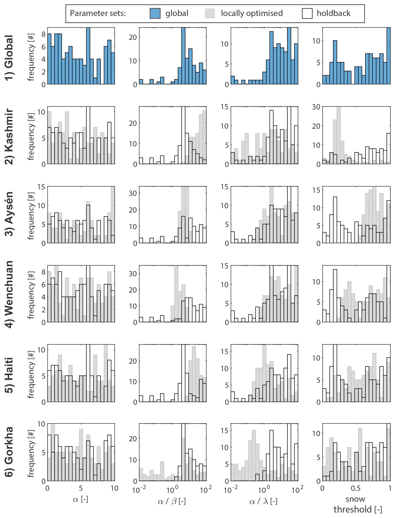
Figure 5 Posterior parameter distributions for the four parameters external to Google Earth Engine after global optimisation (top row) and local optimisation for each earthquake. Rows 2–6 show posterior frequency distributions for each ALDI parameter following local optimisation (grey bars) and the holdback parameter set derived from the global set excluding locally optimised parameters (hollow bars).

ALDI with locally optimised parameters always outperforms the global parameters, and the global parameters always outperform the holdback parameters (Table 3). The difference between local and global parameters is generally larger than between global and holdback parameters. In fact, performance reduction from global to holdback parameters is always < 1 % for AUC. This indicates that the five study sites provide an adequately varied calibration set to enable the generation of a general parameter set that is not overly influenced by any one site. This is encouraging for future blind ALDI application. However, the difference in performance between local and global parameters shows that local optimisation can improve ALDI performance in terms of AUC by up to 9 % (and by 2 % on average). In three cases, one for Kashmir and two for Gorkha, local optimisation improves ALDI to the point where it is no longer outperformed by the manually mapped competitor inventory but instead outperforms it in terms of identifying landslide locations in the check inventory. This is somewhat consistent with the observed divergence of locally optimised parameter distributions from the global distribution at these sites (Fig. 5). However, it likely also reflects the broadly similar performance (i.e. skill) of ALDI and manual mapping at the sites (Table 3).

4.4 Spatial agreement: global comparison to manual mapping

Spatial agreement between manual landslide inventories is surprisingly low not only for the Gorkha study site shown in Fig. 2 but across all sites. TPRs range from 0.08 to 0.8 indicating that at best 80 % and at worst 8 % of the landslide area mapped by one inventory is also identified as a landslide by a second test inventory (Fig. 6a and Table 3). FPRs range from 0.0003 to 0.03, indicating that at best 0.03 % and at worst 3 % of the area that is identified as a non-landslide area in one inventory is instead identified as a landslide by a second test inventory. There are two possible reasons why FPRs are so much lower than TPRs: (1) landslide density is low, so there are few positives (TP+FN) and many negatives (TN + FP) – these are the denominators of TPR and FPR, respectively, amplifying TPR and damping FPR – and (2) landslide mappers may be inherently conservative, mapping only features that they are confident are landslides. TPRs and FPRs are positively correlated but with considerable scatter (Fig. 6a). In some cases manual maps agree quite closely: for example, the inventories of Gorum et al. (2013) and Harp et al. (2016) for Haiti (H_GH, H_HG) or those of Zhang et al. (2016) and Watt (2016) for Gorkha (G_ZW, G_WZ). These cases have a relatively high TPR given their FPR and plot towards the top left of the point cloud in ROC space (Fig. 6a). In other cases the agreement is weaker, such as between the inventories of Li et al. (2014) and Xu et al. (2014) for Wenchuan (W_LX, W_XL), or those of Sato et al. (2007) and Basharat et al. (2016) for Kashmir (K_SB, K_BS). There is a symmetry to the inventory comparison because each inventory takes a turn as the competitor dataset (to which ALDI is being compared) and as the check dataset (against which both are evaluated). As a result, a single pairwise comparison results in two points in Fig. 6a reflecting the switching of roles. The three-way comparison for the Gorkha earthquake results in three pairwise comparisons and six points. When one inventory is considerably more complete and less conservative, then the separation between pairs of points will be large (e.g. Watt and Zhang for Gorkha). Zhang et al. (2017) reported, in their metadata, that their inventory is incomplete and focuses on the largest landslides, while that of Watt (2016) was more complete and less conservative. As a result Zhang et al. (2016) successfully identified only 10 % of the landslide pixels identified by Watt (2016) but identified only a tiny fraction (< 0.1 %) of the study area as landslides when Watt (2016) considered that they were not (G_ZW in Fig. 6a). Conversely, Watt (2016) successfully identified 80 % of the landslides identified by Zhang et al. (2016) but identified a further 1 % of the study area as landslides that were not identified as such by Zhang et al. (2016) (G_WZ in Fig. 6a).

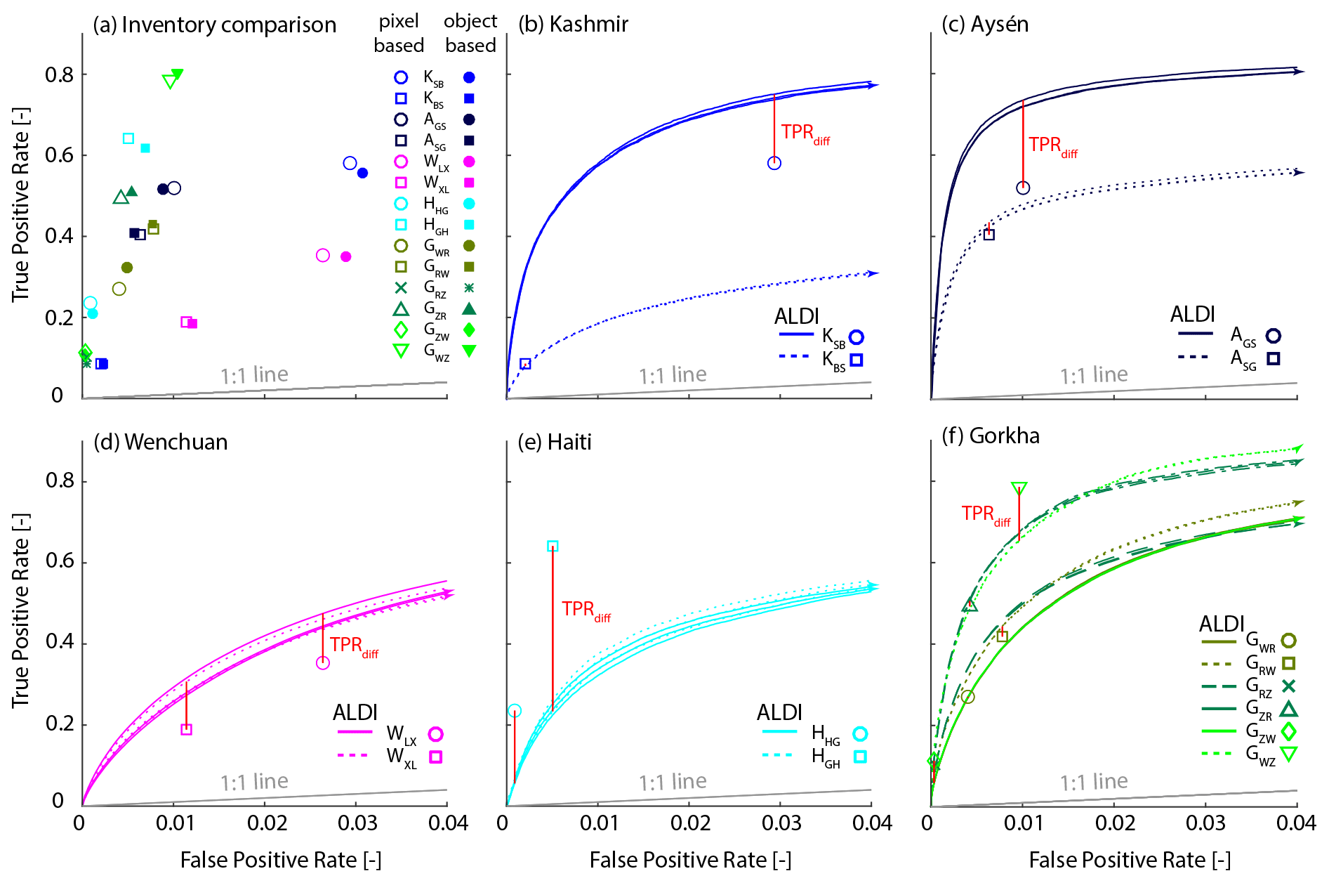
Figure 6 (a) TPR and FPR pairs for the 14 inventory cross comparisons. Open symbols are calculated from a pixel-based analysis at 30 m resolution; solid symbols are calculated from an object-based analysis using mapped polygons. The grey line shows the naïve (random) 1 : 1 relationship. Note the difference in x- and y-axis scales for this and all other panels. (b)–(f) ROC curves for ALDI for each case study. There are three ROC curves for ALDI evaluated against each check inventory (e.g. K_SB) all with the same line style (solid or dashed). In every case the upper curve is from ALDI with locally optimised parameters; the middle curve (indicated with an arrowed end) is from ALDI with global parameters; and the lower curve is from ALDI with holdback parameters. The global and holdback curves are indistinguishable in almost all cases. Red lines indicate the value of TPR_diff, the difference in TPR between ALDI and the competitor inventory when both are evaluated using the same check inventory. Legend acronyms indicate the study site (e.g. K) with the check and then competitor inventory labels as subscripts; see Table 3.

To evaluate ALDI performance relative to manual mapping, we compare the ability of ALDI to successfully identify more landslide pixels in one (check) inventory than another (competitor) inventory when ALDI output is thresholded to reproduce the FPR of the competitor inventory. This TPR difference (TPR_diff) is shown as a red line in Fig. 6b–f; positive differences indicate that ALDI outperforms manual mapping and vice versa. ALDI outperforms manual mapping in the majority of cases when parameters are locally optimised (10 of 14 cases, Fig. 6 and Table 3) and is comparable to manual mapping when a single global-parameter set is applied to all study sites (8 of 14 cases). Performance is only slightly reduced when the test site is held back from the global optimisation, and ALDI continues to outperform manual mapping in 8 of 14 cases.

ALDI performs better at some sites than others, with performances for Aysén and Gorkha particularly good (Table 3). Performance is poor for Haiti, both in absolute terms and relative to the manual mapping. For AUC, an indicator of absolute performance, ALDI performance for the Haiti case is ranked 10th–11th of 14 (where the range results from combining local, global, or holdback tests). Relative to manual mapping, ALDI correctly identifies 51 %–74 % fewer landslide pixels for the same FPR. Explanations for these performance differences are discussed in Sect. 5.4. ALDI in Wenchuan performs only moderately in absolute terms, with ranked performances in the range 9th to 12th out of 14 for AUC, but outperforms manual mapping (1st and 4th for TPR_diff) as a result of the relatively poor agreement between manual maps for the site. Kashmir has very marked differences in ALDI performance depending on the test dataset (all < 4th of 14 for Sato et al., 2007; all > 9th of 14 for Basharat et al., 2016), illustrating the difficulty of interpreting performance relative to check data when the check data themselves contain errors of similar magnitude to the data being tested.

4.5 Area–frequency distributions

Probability density functions (PDFs) for manually mapped landslide areas (Fig. 7a–e) follow a consistent distribution with a roll-over and a heavy right tail that is approximately linear in logarithmic space but that usually has positive (convex up) curvature or a roll-off at very large areas. These characteristics have already been widely reported both for the study inventories in particular (e.g. Gorum et al., 2013; Li et al., 2014; Roback et al., 2018) and for many other landslide inventories worldwide (e.g. Tanyaş et al., 2019). Different inventories for the same study site show broadly consistent scaling in their right tail but tend to differ markedly in the location of the roll-over, modal size, degree of curvature in their right tail, and the location (and presence) of a roll-off for very large areas (e.g. Fig. 7a, d, and e). These differences, as well as their possible explanations, have also been widely reported for these and other sites (see review by Tanyaş et al., 2019).

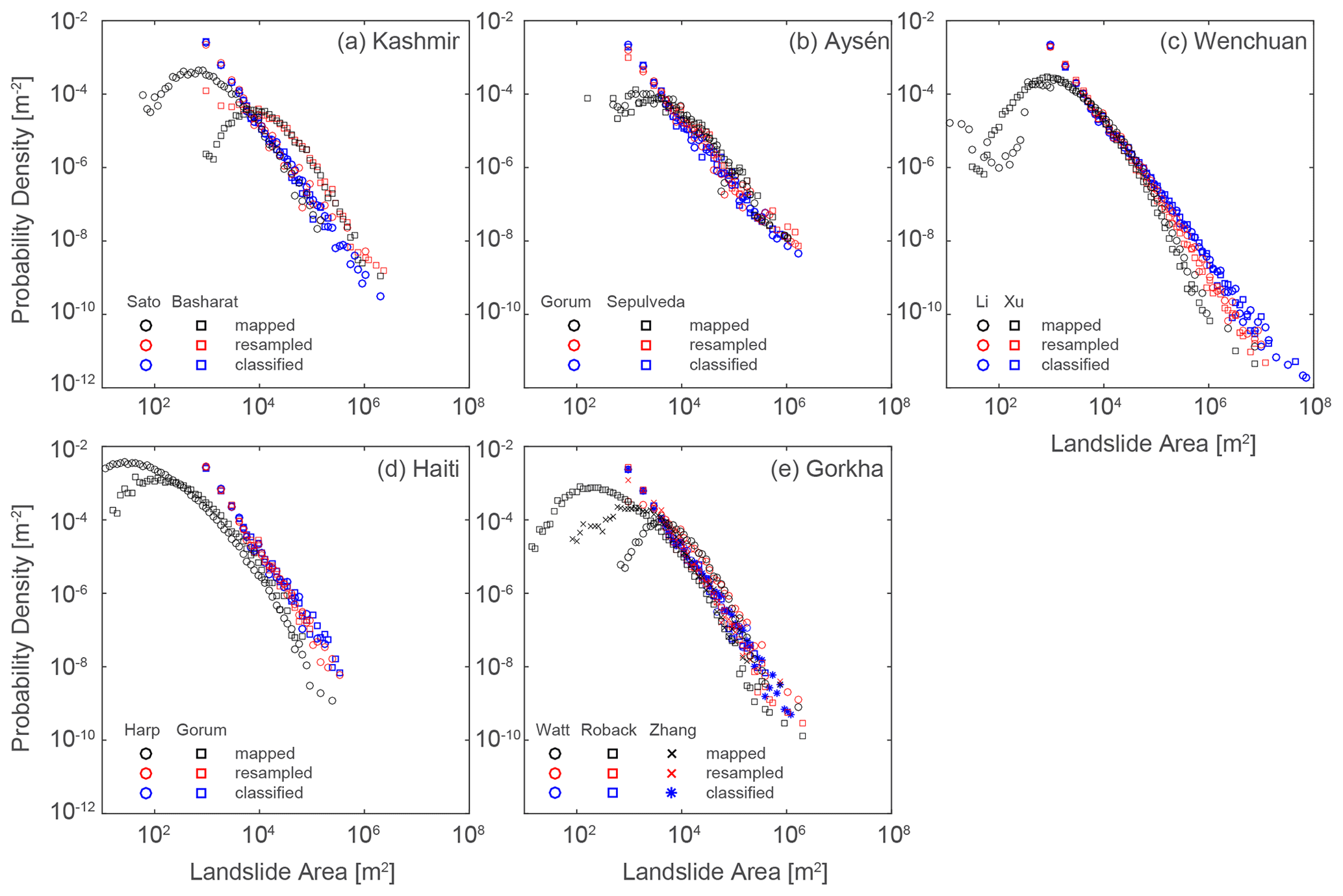
Figure 7 Empirical area–frequency distributions for manually mapped and classified landslides for the five case studies. Manually mapped PDFs are calculated from areas of mapped polygons; resampled PDFs are calculated from patch areas generated from the mapped polygons resampled to a 30 m grid; and classified PDFs are calculated from clustered pixel areas generated by thresholding the ALDI classification values.

The area–frequency distributions derived from ALDI reflect the sizes of clustered landslide-affected areas (rather than the areas of landslide objects themselves). The ALDI-based distributions generally exhibit a broadly similar right tail to those of the manually mapped distributions; both have heavy right tails that closely approximate a power law and have similar scaling (i.e. slope in logarithmic space) in that right tail. However, the ALDI-based distributions are clearly different from those derived from manual mapping, and they lack the following: (1) the roll-over at small areas (in all cases, Fig. 7a–e), (2) the positive curvature to the right tail (particularly clear for Haiti, Fig. 7d), and (3) the roll-off at very large areas (resulting in oversampling of landslides > 10⁵ m² for Wenchuan, Fig. 7c).

These differences can be explained in terms of amalgamation and censoring. The amalgamation of multiple neighbouring landslides increases the frequency of large landslides, fattening the right tail (Marc and Hovius, 2015) and in some cases considerably increasing the size of the largest landslide (e.g. Aysén and Wenchuan, Fig. 7b–c). Resampling to a 30 m grid makes it impossible to record landslides smaller than a single pixel (i.e. 900 m²), censoring them from the area–frequency distribution.

To illustrate the role of amalgamation and censoring we convert the manual landslide maps to binary grids at 30 m resolution, using a majority area rule to identify landslide-affected pixels, and perform the same connected-component clustering used for ALDI. Resampling to 30 m should result in strong censoring and some amalgamation as explained above. Re-clustering with a connected-component algorithm likely results in further amalgamation. Figure 7 shows that resampling and re-clustering manually mapped landslides transforms their area–frequency distributions, removing the roll-over and resulting in distributions that are very similar to those for landslide pixels classified with ALDI. This supports our interpretation that the misfit between ALDI and manual mapping is due to censoring and amalgamation, although we are unable to determine their relative roles. Misfits due to the resolution of Landsat and thus the classification surface are difficult to overcome, whereas improvements in clustering could be more easily implemented.

5 Discussion

5.1 The problem of testing landslide location against uncertain check data

The TPR_diff results for the five study sites show that ALDI outperforms manual mapping in 8 of 14 inventories in terms of its ability to identify landslide-affected areas identified in a second check inventory. This may indicate that ALDI is more skilful than each of these inventories at identifying the locations of landslides. However, because the check inventories are themselves known to contain error, this is not a secure result; erroneous outperformance by ALDI would result if it identified the same artefacts that had been (erroneously) mapped in the check dataset but not in the competitor.

A more secure result can be obtained from the four (of seven) inventory pairs where ALDI outperforms both inventories in the pair when the other is used as check data. This indicates that the ALDI output is more similar to each inventory than the inventories are to one another (Table 3) and demonstrates that ALDI must be more skilful than at least one of the inventories (either the check or competitor inventory) in identifying the locations of landslides. However, we are still unable to conclude whether ALDI is better than one or both inventories or identify which inventory is better. This is because errors in a single inventory influence the result both when it is used as the predictor (i.e. as a competitor against ALDI) and the check dataset (against which both are evaluated).

5.2 Spatial disagreement in manually mapped inventories reflects processing errors, not solely mapping errors

Our findings on the large locational mismatch between co-seismic landslide inventories are initially surprising, given the widespread assumption that such inventories represent a ground truth and the limited attempts to propagate these errors into hazard maps, classification tests, process inferences, or landslide rate estimates. However, the limited number of other studies that do quantify landslide inventory error all suggest very weak spatial agreement between landslide inventories (Ardizzone et al., 2002; Galli et al., 2008; Fan et al., 2019).

The process of generating a landslide inventory from satellite imagery involves choosing which images to map from and how to post-process and georeference them before landslides can be identified and delineated by a human mapper. Thus, the comparison of two inventories is not a direct test of the consistency with which human mappers detect and delineate landslides but instead the consistency with which different research groups generate landslide inventory maps. As an illustration of this distinction, Fan et al. (2019) found that landslide inventories had an overlap of 67 %–86 % (and 76 % on average) when comparing between mappers in the same team mapping from the same imagery. This differs considerably from both our own results (8 %–30 % overlap, Table 3) and other published cross-inventory comparisons (19 %–44 % overlap, Ardizzone et al., 2002; Galli et al., 2008; Fan et al., 2019). In these cases, the inventories being compared were published by independent research groups and were not only collected by different mappers without collaboration but were also generated from different sets of satellite images. For example, Roback et al. (2018) used WorldView imagery with high spatial resolution but which suffers from severe distortions in the Gorkha study area due to the steep landscape and oblique look angles (Williams et al., 2018). Even if landslides were correctly identified in both sets of imagery, differences between inventories could be introduced during georeferencing. Figure 8 shows evidence of the same problem for the Wenchuan inventories, where two sets of mapped landslides with strikingly similar patterns are offset by ∼ 1 km. These georeferencing errors are difficult to attribute to a single inventory and appear to vary in magnitude and direction even over quite short length scales within an inventory (Figs. 2 and 8). Thus, improved performance of ALDI relative to a particular inventory reflects an improved overall workflow rather than specifically the ability to identify landslides in images.

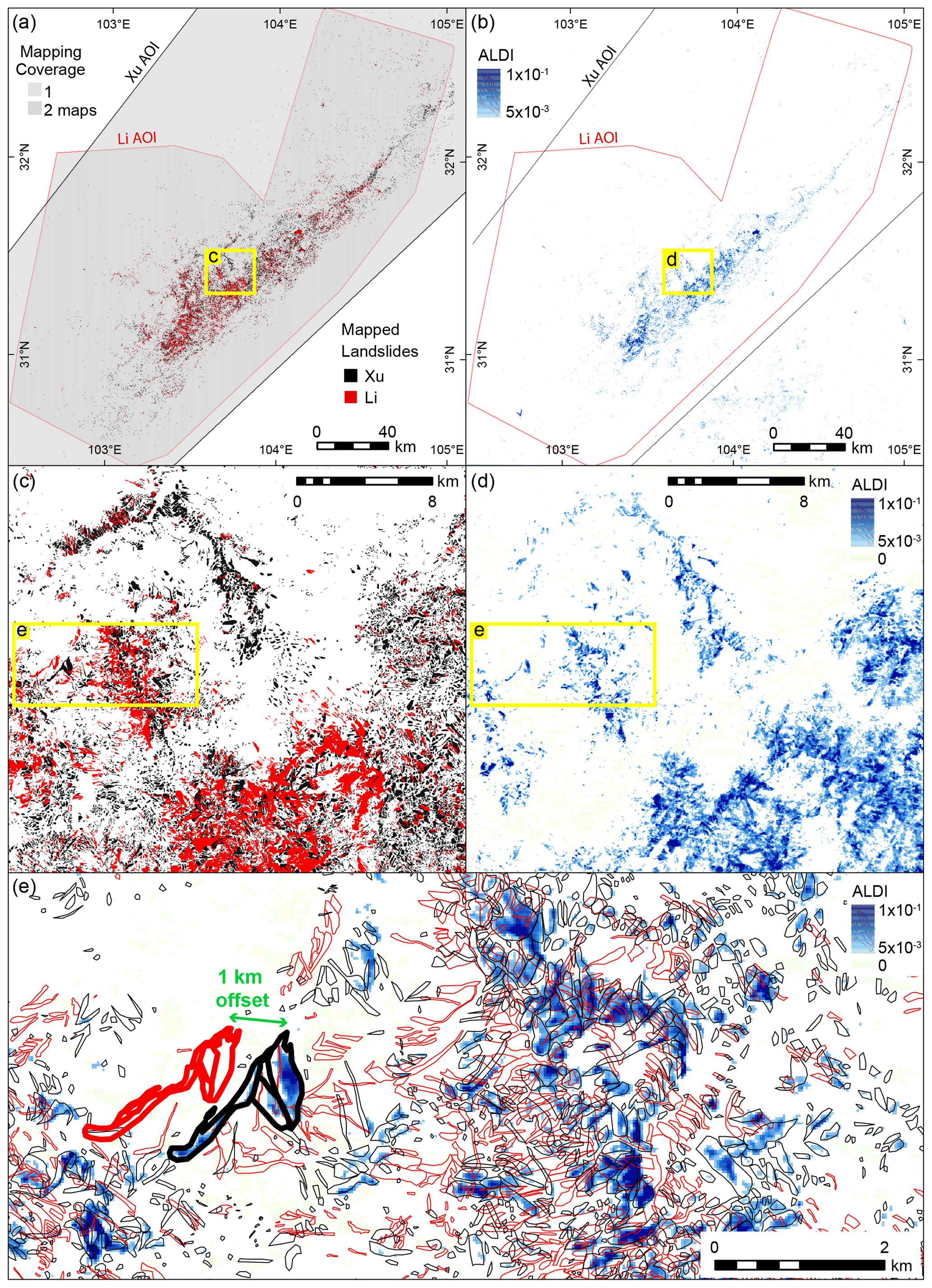
Figure 8 Manually mapped landslides and ALDI classifier results for the Wenchuan study site. (a) Mapped landslides at the scale of the full study area with AOIs shown in grey; Xu and Li refer to the inventories of Xu et al. (2014) and Li et al. (2014), respectively. (b) ALDI values for the full study area. (c) Mapped landslides and (d) ALDI values for a subset of the study area. (e) Detailed view of mapped landslides overlain on ALDI values. Yellow boxes in each panel show the locations of nested panels (e.g. c in a and d in b). Thicker outlines in panel (e) indicate landslides of very similar geometry that are offset by ∼ 1 km in the different inventories; the ALDI pattern suggests that the map by Xu et al. (2014) is more likely to be correctly georeferenced in this case.

5.3 Limitations to ALDI performance

ALDI performance varies from site to site, with particularly good performances for Aysén and Gorkha but particularly poor ones for Haiti. The overall poor performance for Haiti may reflect the drier conditions in the study area, which lead to vegetation that is more difficult to differentiate from landslide scars, or the higher degree of human influence on land cover relative to other sites, which may result in more vegetation changes not related to landslides. ALDI can identify landslides only in areas where they result in a change in NDVI and will perform better in areas where this change is more pronounced (all else being equal). This will occur where pre-event NDVI is higher due to denser and/or more vigorous vegetation coverage, both of which result in a larger share of reflectance from leaves, with their more pronounced “red edge” (the red–near-infrared reflectance change). Conversely, ALDI will perform poorly in areas with sparse vegetation such as the epicentral area of the 2010 Sierra Cucapah earthquake (Barlow et al., 2015).

Poor performance for Haiti in comparison with the manual mapping may also be due to ALDI's coarse 30 m resolution relative to the dimensions of the landslides in the study area. ALDI will identify a pixel as landslide-affected only if the landslide occupies enough of the pixel to alter its spectral response and will perform better when landslides are large enough to occupy large fractions of one or many pixels. Given their typically elongate shape (Taylor et al., 2018), landslides with widths < 30 m and thus areas < 2700 m² (assuming $L/W=$ 3, 75th percentile from Taylor et al., 2018) will be partially censored, with the degree of censoring increasing as width declines. Median landslide area in the inventories examined here ranges from 250 m² for Haiti (Harp et al., 2016) to 19 000 m² for Kashmir (Basharat et al., 2016), with medians less than 2700 m² in 4 of 14 inventories. Therefore, this censoring will strongly affect ALDI-derived inventories, particularly in areas with lower relief (such as Haiti) where smaller landslides are expected to be more common (Jeandet et al., 2019).

Finally, poor performance for Haiti is also likely to reflect the limited number and quality of Landsat images acquired over the study area. ALDI used imagery from 2005–2012 to identify landslides triggered by the Haiti earthquake and thus relies exclusively on Landsat 5 and Landsat 7 data (Landsat 8 launched in 2013). Both Landsat 5 and Landsat 7 are problematic for this study site and period. All of the Landsat 7 data contain data gaps due to Scan Line Corrector (SLC) failure from June 2003 onwards, and only small amounts of Landsat 5 data for areas outside the USA were retained during this period, limiting archival imagery in some areas (see Fig. S5 in Pekel et al., 2016). For Haiti the pre-earthquake stack is composed of 6 Landsat 5 images and 205 Landsat 7 images and the post-earthquake stack of 16 and 91 images, respectively. Limited availability of Landsat 5 data at this site means that in some areas the classifier relies exclusively on Landsat 7 and is thus unable to calculate an ALDI value for pixels within the data gaps (these are visible as white stripes in the eastern half of Fig. 9b). While some areas of high ALDI values show good agreement with mapped landslides, there are also large patches of high ALDI values with complex shapes that are uncharacteristic of landslides and that manual mapping shows as likely false positives (Fig. 9c).

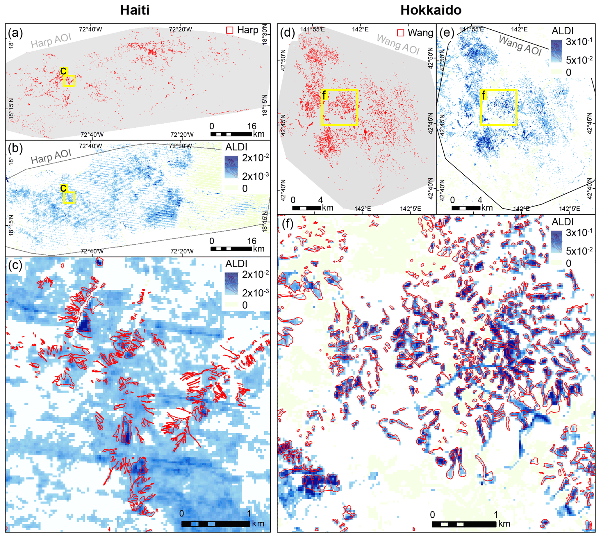
Figure 9 Mapped landslides and the ALDI classifier for the Haiti (left) and Hokkaido (right) study sites. (a) Mapped landslides from Harp et al. (2016) in Haiti at the scale of the full study area with the associated AOI shown in grey. (b) ALDI values for the full study area; the yellow box shows the location of panel (c). (c) ALDI values overlain by mapped landslides from Harp et al. (2016) for a subset of the study area. (d) Mapped landslides from Wang et al. (2019) in Hokkaido at the scale of the full study area with the associated AOI shown in grey. (e) ALDI values for the full study area. The yellow box shows the location of panel (f). (f) ALDI values overlain by mapped landslides from Wang et al. (2019) for a subset of the study area. ALDI uses Landsat 5 and Landsat 7 for Haiti and Sentinel-2 for Hokkaido, both gridded at 30 m resolution.

Given these limitations to Landsat 5 and Landsat 7 imagery, it is perhaps surprising that ALDI performs so well in the Aysén case (where the stack extends from 2002–2009). This is likely due to the larger number of Landsat 5 images available for the study site (140 in the pre-earthquake stack and 46 in the post-earthquake stack) and to the location of the area of densest landsliding near the centre of a Landsat 7 image where data gaps related to SLC failure are minimised. The 2015 Gorkha earthquake is the only case study for which Landsat 8 data were available, perhaps explaining the relatively good performance at this site and offering hope for application to more recent events.

Sparse image data (associated with incomplete archiving of Landsat 5) and sensor problems (primarily SLC failure on Landsat 7) from 2003–2014 suggest ALDI-based mapping in this period should be handled with care. However, the majority of our test earthquakes come from this period, and we have demonstrated that even with these constraints, ALDI performs well in determining landslide locations for four of the five case studies, both in absolute terms and relative to manual mapping. Potential checks on ALDI applications during this time period could entail careful checking of the numbers of images in the pre- and post-earthquake stacks, the extent of Landsat 7-derived striping in the ALDI map, and the size and shape of the landslides in the ALDI-derived inventory. Small image stacks (particularly for Landsat 5), extensive striping, and large complex landslide shapes should all be treated as indicators of potentially poor ALDI performance. However, even when large image stacks are available for an earthquake-affected area, cloud cover can limit the number of usable observations per pixel within the pre- and post-earthquake stacks.

ALDI can identify landslide-affected pixels with a high degree of skill (comparable to manual mapping) but is considerably less skilful in identifying discrete landslides, as demonstrated by the difference in ALDI and manually mapped area–frequency distributions. As with Parker et al. (2011), additional steps are required to identify separate landslides (e.g. Marc et al., 2016). Calibration based on a small subset of manually mapped landslides followed by subsequent manual editing to remove false positives could result in a very good inventory in a fraction of the time associated with full manual mapping.

5.4 Strengths and weaknesses of ALDI relative to manual mapping

The most widely used properties of landslide inventories are landslide location and geometry (Guzzetti et al., 2012). In terms of location, ALDI performs comparably to manual mapping in identifying whether the majority of each pixel in a 30 m grid is landslide-affected. However, it performs worse in capturing landslide area–frequency distributions, primarily because it cannot identify small isolated landslides (i.e. with areas < 900 m² separated by more than 30 m), and separating the output from ALDI (or any other pixel-based classifier) into discrete landslide objects is not straightforward.

Current approaches to train and test landslide prediction models (including hazard and susceptibility models) almost exclusively use pixel-based information on landslide presence or absence rather than information about the size or shape of a landslide at a particular location (see Bellugi et al., 2015, for an exception). For such applications, skilful identification of landslide-affected pixels is the sole requirement. Our results suggest that the ALDI landslide inventory would be an appropriate product to use in these cases, as it is better than at least one of the manual inventories in four of the five case studies (Table 3).

Landslide geometry is required to construct landslide area–frequency distributions and is useful to distinguish landslide initiation and runout zones (Marc et al., 2018). Manual mapping provides landslide geometry with a high level of accuracy, although disagreements in landslide area–frequency distributions for manually mapped inventories have already been reported, with the most pronounced differences being in roll-over location, usually due to differences in image resolution (Galli et al., 2008; Fan et al., 2019; Tanyaş et al., 2019). The accuracy of landslide geometry derived from ALDI depends strongly on the extent to which landslide pixels can be clustered to identify separate landslides (e.g. Marc et al., 2016) and on the pixel resolution. The first of these is common to all pixel-based classifiers. Given the relatively coarse resolution of the underlying Landsat data, we expect ALDI-derived geometries to be accurate only for large landslides, as shown in Fig. 7.

All in all, we expect ALDI to be useful in identifying areas for further (more detailed) mapping at multiple scales: (1) globally, as a supplement to the existing archive of co-seismic landslide inventories by examining historic events for which a landslide inventory has never previously been generated but where landslides are known or expected to have been triggered; (2) at a site, to identify areas of interest or to extend the study area beyond that which can be feasibly mapped by hand; and (3) at the finest scale, to identify individual candidate landslides to be manually checked and re-digitised if necessary. We also expect ALDI to be a useful check on manual mapping, enabling increased homogeneity in areas where there is only patchy coverage of high-resolution imagery and perhaps for identifying georeferencing errors.

We do not expect ALDI in its current form to be as useful as manual mapping: (1) as a source of rapid landslide information to inform emergency response (because ALDI performs better with 2 years of post-event images); (2) for size or shape distributions (because of censoring and amalgamation inherent in 30 m pixel-based output); (3) for analysis where landslide initiation zones must be differentiated from runout; (4) in landscapes where vegetation is sparse (because NDVI changes in landslide pixels are unlikely to be detectable relative to natural variability); and (5) in landscapes where small landslides are widely distributed across the landscape (because the pixel-averaged NDVI change will be small if only a fraction of a pixel is disrupted).

5.5 Comparison to other automated detection methods

Automated detection of landslides typically relies on vegetation change detection and involves either generating indices of surface disturbance from which landslides can be manually identified (e.g. Scheip and Wegmann, 2021) or performing a supervised classification (e.g. Barlow et al., 2003; Behling et al., 2014, 2016; Prakash et al., 2020).

A recent example of automated surface disturbance detection, HazMapper (Scheip and Wegmann, 2021), uses similar image data (Landsat) and the same platform (Google Earth Engine) as ALDI but for a different purpose and using different functions to combine and transform the imagery. HazMapper is designed to generate a qualitative metric for surface change rather than a landslide-specific mapping tool. As a result, the approach does not mask snow-covered areas in case these are of interest for a user's particular application. The approach is simpler than that of ALDI in that HazMapper calculates the NDVI difference only, rather than accounting for post-event NDVI, seasonal variability, and noise in the NDVI signal for each pixel. It is currently only applied to Landsat 7 onwards and only for individual sensors, rather than combining images from multiple Landsat sensors. This limits the events that can be examined to those occurring after 1999. However, results from HazMapper for the same study periods examined here show a good qualitative agreement with the ALDI results. The similarity in approach, using stacks of Landsat imagery before and after a suspected trigger event, means that the two approaches will likely have many of the same strengths (e.g. the accurate georeferencing of Landsat imagery) and limitations (e.g. the coarse resolution of Landsat imagery and long wait times required to generate the post-event stack).

Alternative approaches to landslide detection that involve supervised classification typically rely on machine learning (e.g. Prakash et al., 2020) or clustering methods (e.g. Barlow et al., 2003; Behling et al., 2014; 2016). These more complex approaches are compatible with the data and platforms that we use here. Although we have taken a simpler approach, the classification surfaces generated by ALDI could be coupled with modern machine learning approaches to improve ALDI's landslide detection skill. However, our results also highlight an important potential limitation to the use of supervised learning for landslide detection in general. Given the very severe disagreement between manually mapped landslide inventories, any supervised learning method will have a very high risk of propagating gross errors into the classifier unless the training inventory is precisely co-located with the imagery used by the classifier. ALDI could help improve existing supervised classification efforts by providing additional well-referenced landslide inventories or by correcting existing ones.

5.6 Application to future earthquakes

The increased frequency and quality of optical imagery suggest that ALDI should perform well for future earthquakes. In particular, Sentinel-2 imagery can generate NDVI at 10 m spatial resolution (Table 1). The two Sentinel-2 satellites were launched between June 2015 and March 2017, and thus there is a limited stack of pre- or post-earthquake images available to date. The 2018 Hokkaido earthquake offers the best trade-off to date between pre- and post-event data. As a test of the wider applicability of ALDI to future events, we ran ALDI using the global-parameter set identified above and evaluated its results against landslides mapped from aerial imagery by Wang et al. (2019). The results are extremely promising both at the scale of the entire epicentral area (Fig. 9d and e), as well as of individual landslides, with few false positives, a large area under the ROC curve (0.94), and many landslides clearly delineated by a sharp break from high to low ALDI values (Fig. 9f).

6 Conclusion

Rapid derivation of landslide inventories after large triggering events remains a key research challenge. We have developed a parsimonious automatic landslide classifier, ALDI, that uses pre- and post-event stacks of freely available medium-resolution satellite imagery and relies on landslide-induced changes to vegetation cover and thus to NDVI values. We test the classifier against multiple independent manually mapped inventories from five recent earthquakes. Considering that manually mapped inventories are typically assumed to be the ground truth against which automatic classifiers are evaluated, we find that agreement between different manual inventories is surprisingly low (8 %–30 % of landslide area in common). ALDI often identifies landslides in one inventory missed in the other and even identifies some candidate landslides not in either inventory but that have location and morphometric characteristics that strongly suggest they are true positives.

We further find that ALDI can identify landslide locations with a level of skill that is comparable to manual mapping on a pixel-by-pixel basis. ALDI calibrated to mapped landslides at a site outperforms manual mapping in 10 of 14 cases (i.e. 71 %). The only cases where manual mapping performs better are the two inventories for the 2010 Haiti earthquake, where the stack of available Landsat images is extremely limited, and the cross comparison of inventories for the 2015 Gorkha earthquake, where strong agreement between inventories is the result of mapping from very similar satellite imagery.

Even when using a global-parameter set, ALDI outperforms manual mapping in 8 of 14 cases (57 %) with 10 of 14 cases (71 %) performing either better than manual mapping or within the uncertainty in manual mapping performance estimates. These results suggest that ALDI can be applied with considerable confidence to map the areas affected by co-seismic landslides in future earthquakes without the need for additional calibration. Holdback tests do not change either of these statistics and affect our chosen performance metrics by only a few percent, suggesting that the set of earthquakes that we have used is large enough to develop a robust global-parameter set.

The area–frequency distributions for clusters of pixels that are classified as landslides both from manual and automated landslide classification are broadly similar, particularly in their heavy right tail. However, the classifier-derived inventories are fundamentally limited by the resolution of the imagery and their inability to disaggregate amalgamated landslides so that an object-based approach is required to recover realistic area–frequency information.

ALDI is fast to run, uses free imagery with near-global coverage, and generates landslide information that is of comparable quality to that of costly and time-consuming manual mapping, depending on its intended use. Thus, even in its current form it has the potential to significantly improve the coverage and quantity of landslide inventories. However, its simplicity (performing only pixel-wise analysis) and parsimony of inputs (using only optical imagery) suggest that considerable further improvement should be possible.