Landsifier v1.0: a Python library to estimate likely triggers of mapped landslides

Landslide hazard models aim at mitigating landslide impact by providing probabilistic forecasting, and the accuracy of these models hinges on landslide databases for model training and testing. Landslide databases at times lack information on the underlying triggering mechanism, making these inventories almost unusable in hazard models. We developed a Python-based unique library, Landsifier, that contains three different machine-Learning frameworks for assessing the likely triggering mechanisms of individual landslides or entire inventories based on landslide geometry. Two of these methods only use the 2D landslide planforms, and the third utilizes the 3D shape of landslides relying on an underlying digital elevation model (DEM). The base method extracts geometric properties of landslide polygons as a feature space for the shallow learner – random forest (RF). An alternative method relies on landslide planform images as an input for the deep learning algorithm – convolutional neural network (CNN). The last framework extracts topological properties of 3D landslides through topological data analysis (TDA) and then feeds these properties as a feature space to the random forest classifier. We tested all three interchangeable methods on several inventories with known triggers spread over the Japanese archipelago. To demonstrate the effectiveness of developed methods, we used two testing configurations. The first configuration merges all the available data for the k-fold cross-validation, whereas the second configuration excludes one inventory during the training phase to use as the sole testing inventory. Our geometric-feature-based method performs satisfactorily, with classification accuracies varying between 67 % and 92 %. We have introduced a more straightforward but data-intensive CNN alternative, as it inputs only landslide images without manual feature selection. CNN eases the scripting process without losing classification accuracy. Using topological features from 3D landslides (extracted through TDA) in the RF classifier improves classification accuracy by 12 % on average. TDA also requires less training data. However, the landscape autocorrelation could easily bias TDA-based classification. Finally, we implemented the three methods on an inventory without any triggering information to showcase a real-world application.

1 Introduction

Landslides are gravitational movements of rock and debris that pose a severe threat to the human environment (Depicker et al., 2021). Hazard models are developed to forecast landslides or to aid in understanding landslide processes to mitigate their undesired consequences (Lombardo et al., 2020). These models commonly rely on mapped landslides to assess the relevant landslide causes in combination with landslide triggers, i.e., earthquake and rainfall (Lombardo and Tanyas, 2021; Ozturk et al., 2021; Marin et al., 2020). However, many historical landslide inventories lack information about the triggering mechanism, decreasing their potential utility in models (Bíl et al., 2021; Martha et al., 2021). More recent semi-automated satellite-based landslide mappers also often disregard the triggering information (Behling et al., 2014, 2016; Ghorbanzadeh et al., 2019), except the event-based inventories–landslide-mapping campaigns following a precursory triggering event such as a strong earthquake (Stumpf and Kerle, 2011; Gorum et al., 2014). Using landslide inventories with missing triggers could introduce biases as it is possible to accidentally use an earthquake-triggered inventory to assess rainfall-induced landslide hazards and vice versa. Hence, classifying the trigger of entire landslide inventories or mapped individual landslides would enhance the usability of newly acquired and historical inventories in landslide models (Guzzetti et al., 2012).

Landslide planforms are used to estimate the mobilized landslide volume, for example, estimating the potential sediment budget of a large-landslide-triggering event (Malamud et al., 2004; Fan et al., 2012). This type of scaling relationship between the area of landslide planforms to mobilized landslide volume allows comparing the impact of different landslide triggers, such as human versus earthquakes, in terms of the landslide-triggered influence on landscape (Tanyaş et al., 2022). However, this area–volume scaling depends on the triggering mechanism of landslides. For example, an earthquake-triggered landslide has a different area–volume relationship than a rainfall-induced landslide. Hence, extracting the landslide trigger information could enhance the estimation capacity of landslide volumes (Moreno et al., 2022) and also help predict the size of co-seismic landslides for a given earthquake (Lombardo et al., 2021). Also, when the exact trigger is known, observed landslides help assess earthquakes' ground motion patterns when no seismic observation is available (Lombardo et al., 2019).

Landslides with the same trigger morphologically cluster, for example, covering narrowly the available statistical variability of hillslope angles in a study region (e.g., Jones et al., 2021), and, thus, could have characteristic shapes reflecting their triggering mechanism, for instance, by having similar area and perimeter ratio or size (Taylor et al., 2018; Samia et al., 2017). We developed a binary classifier that groups landslides either as earthquake-triggered or rainfall-induced based on this hypothesis (Rana et al., 2021). This initial model demonstrated that the landslides with an identical trigger indeed exhibit similar geometric properties. Thus, finding the trigger of landslides is a classification problem, and one can employ machine-learning tools to carry out automated classification of landslide triggers. In each classification problem, the principal idea is to construct a classifier based on training samples and evaluate its performance on testing samples. The classifier predicts the class y corresponding to the input sample x. These input samples x can be one-dimensional vectors or images; for instance, in a soil classification problem (e.g., Bhattacharya and Solomatine, 2006), x is a one-dimensional vector, and in any image classification problem, x is an image (2D or multi-dimensional matrix) (Domingos, 2012).

Our preliminary model (Rana et al., 2021) can classify landslide triggers by only using the geometric properties of landslide polygons. Here, we introduce two additional methods for landslide trigger classification. In one new method, we treated landslide polygons as images, and these images are fed as the sole predictor to a deep learner – convolutional neural networks (CNNs). Treating landslide polygons as images eases the workflow as an image already resembles some of the geometric features of the first method. Both of these methods rely on two-dimensional (2D) landslide planforms, ignoring the three-dimensional (3D) shapes of real-world landslides. In another approach, we included the 3D shapes of landslides by incorporating the elevation of landslides via a digital elevation model (DEM). In this approach, we extracted the topological features of these 3D shapes using a recently developed technique known as topological data analysis (TDA). These topology-based features are input to the decision-tree-based shallow learner as in the first method. We included the TDA-based model considering its potential to handle other relevant classification problems in future versions of our tool, e.g., classifying landslide types (Cruden and Varnes, 1996; Varnes, 1978). The above-listed methods could be used independently following similar script streams.

This study also introduces a new Python library, Landsifier, that classifies the trigger of landslides, individually or as a whole, in an inventory where the landslide source mechanism is undocumented. Landsifier is the first-ever library built for estimating likely triggers of mapped landslides; the methods used in this library to find landslides' triggers are new. Two of these methods are introduced in this paper for the first time, while the third was published in our preliminary work (Rana et al., 2021). The library consists of three different machine-learning-based methods mentioned above; we elaborate on these methods in Sect. 3. Various functionalities of the library are described in Sect. S2, where we also list several supporting functions to calculate landslide polygons' geometric properties, convert landslide polygons' shape to a binary-scale image, download a digital elevation model (DEM) corresponding to inventory location, and evaluate the diagnostic performance of the final classification. To demonstrate the efficacy of the developed methods, we apply each to six landslide inventories with known triggers spread over the Japanese archipelago and document our findings in Sect. 4. In Sect. 6, we further highlight the weaknesses of each method to ease choosing the suitable classifier for the various applications.

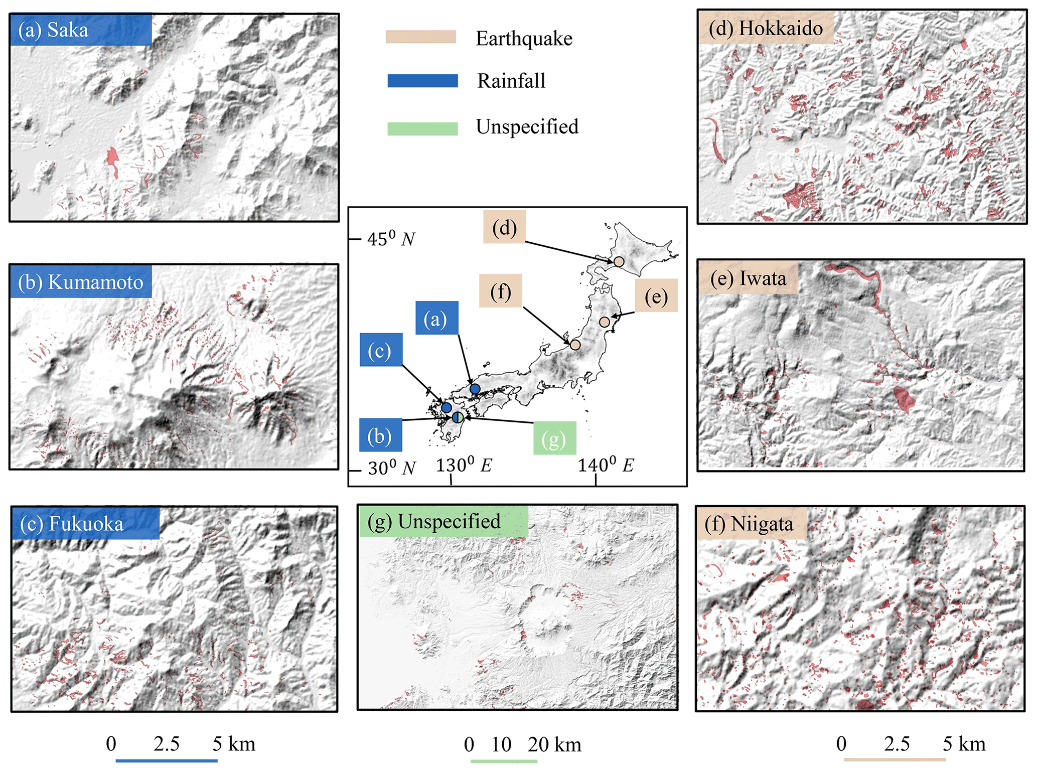
Figure 1 The seven landslide inventories used in this work are spread over Japan, and their geographical locations are shown on the country's map at the center of the figure. Panels (a)–(g) show the subset of landslide polygons highlighted in red on local hillshades. (a–c) Rainfall-induced inventories; (d–f) coseismic inventories; (g) undocumented “Kumamoto unspecified” inventory.

2 Data

In this work, we used seven landslide inventories spread over the Japanese archipelago (Fig. 1). The trigger mechanism of six out of seven landslide inventories is known (Fig. 1a–f), whereas the last inventory has no documented triggering information (Fig. 1g). We use the last inventory to demonstrate the practical deployment of the final model as this case represents the model's real-world usage. Out of six landslide inventories, three inventories are earthquake-triggered (Fig. 1d–f) and are associated with the 2018 M_w 6.6 Hokkaido Eastern Iburi (3256 landslides), the 2008 M_w 6.9 Iwate–Miyagi Nairiku (4160 landslides), and the 2004 M_w 6.6 Niigata (8780 landslides). The remaining three are rainfall-induced (Fig. 1a–c), and these are associated with the 2017 Fukuoka northern-Kyushu torrential rainfall disaster (1924 landslides); the 2018 Saka, Japan, floods (2817 landslides); and the Kumamoto inventory (5564 landslides) that is collected over 1992–2012, which is not associated with any particular event.

The Geospatial Information Authority of Japan (GSI) is the source of the Hokkaido Eastern Iburi earthquake (September 2018), Fukuoka rainfall (July 2017), and Saka rainfall (July 2018) inventories. The source of the other two coseismic inventories – Iwata and Niigata – is the global repository created by Schmitt et al. (2017). The remaining two inventories from the Kumamoto region are provided by Japan's National Research Institute for Earth Science and Disaster Resilience (NIED). The first inventory from Kumamoto is associated with rainfall (Fig. 1b), whereas the second inventory is without any triggering information (Fig. 1g). Hereafter, we refer to this second inventory as “Kumamoto unspecified” (it consists of 612 landslides with unknown triggers).

The TDA-based method uses elevation data to obtain the 3D shapes of landslides from their 2D planforms. We use the Shuttle Radar Topography Mission (SRTM) digital elevation model (DEM) data that come with a spatial resolution of approximately 30 m. The SRTM data are freely available from https://www2.jpl.nasa.gov/srtm/ (last access: 17 November 2022) by manually selecting the tiles which correspond to topographic quadrangles. Each tile covers 1^∘ of both the latitude and longitude region. The Landsifier library automatically downloads the corresponding tile(s) covering the region of the landslide inventory used (explained further in Sect. S2).

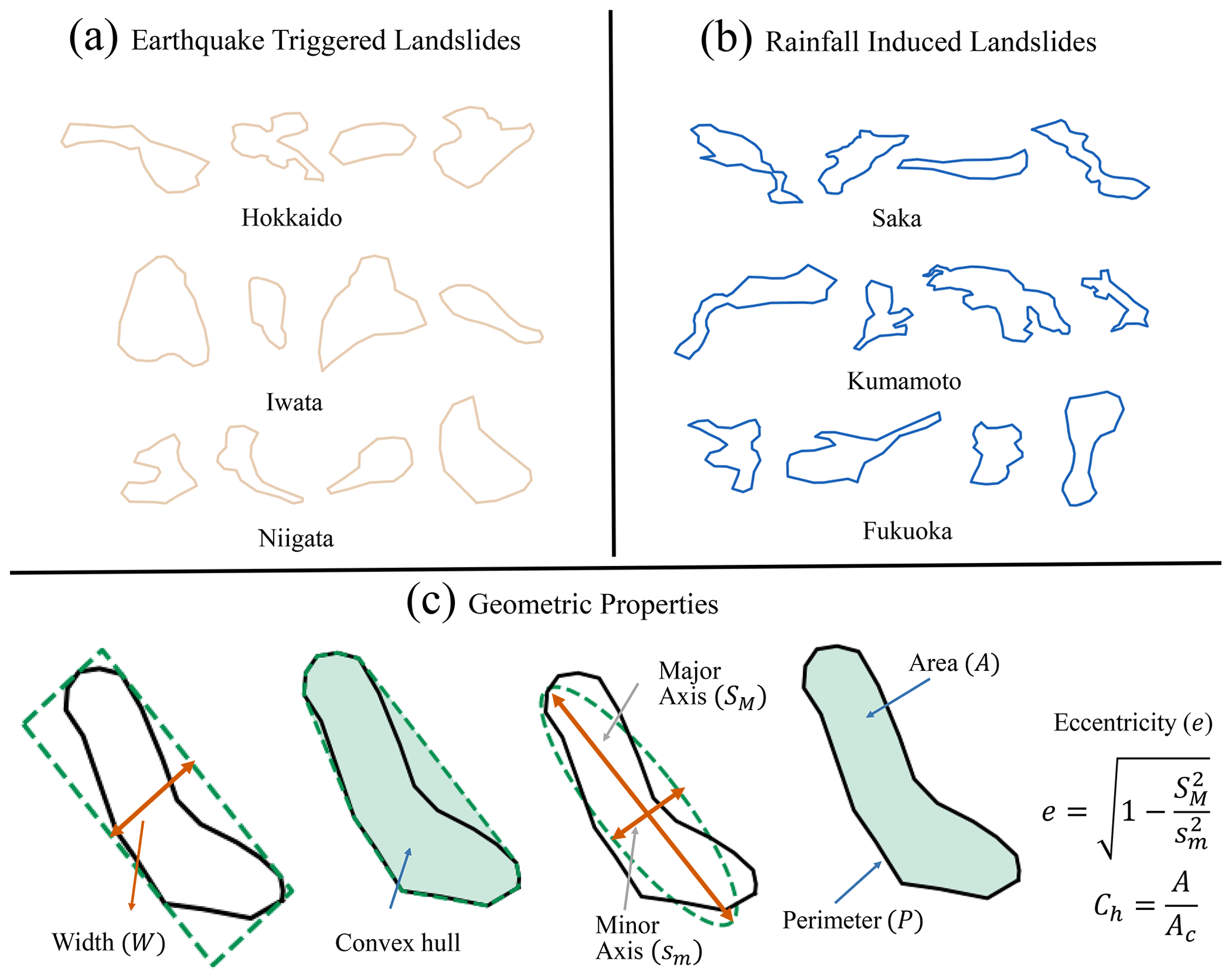
Figure 2 Sample landslide planforms from all six known triggered inventories. (a) Earthquake-triggered inventories. (b) Rainfall-induced inventories. (c) Geometric properties of the landslide polygon (from left to right): width (W) of the minimum area bounding box fitted to the polygon, convex-hull-based measure (C_h), minor (s_m) and major (S_M) axis of an ellipse fitted to the polygon having area A and perimeter P.

3 Methods

In our preliminary study (Rana et al., 2021), we introduced a method that can classify landslide triggers by only using geometric features of landslide planforms. This initial model constitutes the first method in the Landsifier library, and for continuity, we briefly describe it in section 3.1. In this paper, we further diversify our initial model and introduce two new methods. One new method is based on the topological features of 3D shapes of landslides computed using TDA, described in Sect. 3.2. The other new method uses CNN to carry out an image-based classification of landslide triggers; see Sect. 3.3. We anticipate that the variety of methods and corresponding Python library presented here will allow researchers to perform this analysis seamlessly.

3.1 First method: geometric-feature-based classification

In the first method, we used the geometric properties of 2D landslide polygons for the classification. We explored several geometric properties of landslide polygons (e.g., Fig. 2). Using a combination of feature selection methods and feature importance analysis, for instance, removing highly correlated features, we choose the seven geometric properties of polygons that lead to optimum results. These geometric features are area A; perimeter P; convex-hull-based measure $C_{\mathrm{h}}=\frac{A}{A_{\mathrm{c}}}$, where A_c is the area of the convex hull fitted to the polygon (hereafter, we will refer C_h as a convex hull measure); the ratio of area to perimeter $\frac{A}{P}$; the width of the minimum area bounding box W; minor axis s_m; and eccentricity of the fitted ellipse e having area A and perimeter P. All these seven geometric features are calculated using the Python library shapely (Gillies, 2013). The feature vector ([A, P, C_h, W, s_m, $\frac{A}{P}$, e]) is the input variable to a machine-learning algorithm – random forest (described in the Sect. S1 in the Supplement). Further details of the method can be found in Rana et al. (2021).

In Rana et al. (2021), we analyzed the distributions of geometric properties of the earthquake and rainfall polygons and found geometric dissimilarities between earthquake and rainfall polygons' shapes. Earthquakes polygons are more likely to have a compact shape (as measured by convex-hull-based measure) than rainfall polygons. Moreover, earthquake polygons have more chances to have a larger area (A), perimeter (P), the ratio of the area to the perimeter ($\frac{A}{P}$), and minimum width (W) than rainfall polygons. In contrast, rainfall polygons have a larger eccentricity (e) than earthquake polygons of an ellipse fitted to the polygon. Rainfall polygons are more sinuous in shape, leading to the smaller minor axis and larger major axis leading to the larger eccentricity of the ellipse fitted to the polygon (Rana et al., 2021).

Figure 3 Sample 3D landslides from six known triggered inventories. (a) Flowchart of conversion of 2D landslide planforms to 3D landslide shape. (b) Earthquake-triggered 3D landslide samples; (c) rainfall-induced landslide 3D samples. The 2D landslide planforms converted to 3D landslide shapes by using the elevation of landslides through a digital elevation model (DEM).

3.2 Second method: topological-feature-based classification

In the second method, we used the 3D shapes of landslides by incorporating the elevation data of the landslide regions. We extracted geometrical and topological properties of a landslides' 3D shapes using topological data analysis (TDA) and then used these properties as a feature space for the machine-learning algorithm – random forest (described in Sect. S1). The topological properties of the landslide's 3D shape extracted using DEM provide additional insights into the landslide triggers, which might further improve the accuracy of the landslide trigger classification. We converted the 2D landslide polygons to 3D landslide polygons using interpolation of 30 m elevation data (DEM) around the bounding box of landslides. We took only the elevation data within the landslide polygons to preserve the geometric shape of the landslides (Fig. 3). We explored various TDA features to quantify the 3D shapes of landslides using the Python library giotto-tda (Tauzin et al., 2021). Using random forest feature importance analysis, we selected the top 10 most relevant features, as irrelevant features increase the complexity of the model and are ineffective in improving the classification results. These selected relevant features constitute the input variables for the random forest classifier.

Topological data analysis (TDA) provides a gamut of metrics to quantify the multidimensional shape of data by applying techniques of algebraic topology (Carlsson, 2009). These metrics could also serve as a feature space for machine-learning algorithms to solve classification problems, e.g., the classification of manifolds or complex geometric shapes. The central idea of TDA is persistent homology that identifies persistent geometric features in the data; it uses simplicial complexes to extract topological features from the point cloud data. A simplicial complex is a collection of simplexes and building blocks of higher-dimensional counterparts of a graph. For example, a point is a zero-dimensional simplex, an edge which is a connection between two points is a one-dimensional simplex, and a filled triangle formed by connecting three non-linear points is a two-dimensional simplex. In general, an n-dimensional simplex is formed by connecting n+1 affinely independent points (Munch, 2017; Garin and Tauzin, 2019).

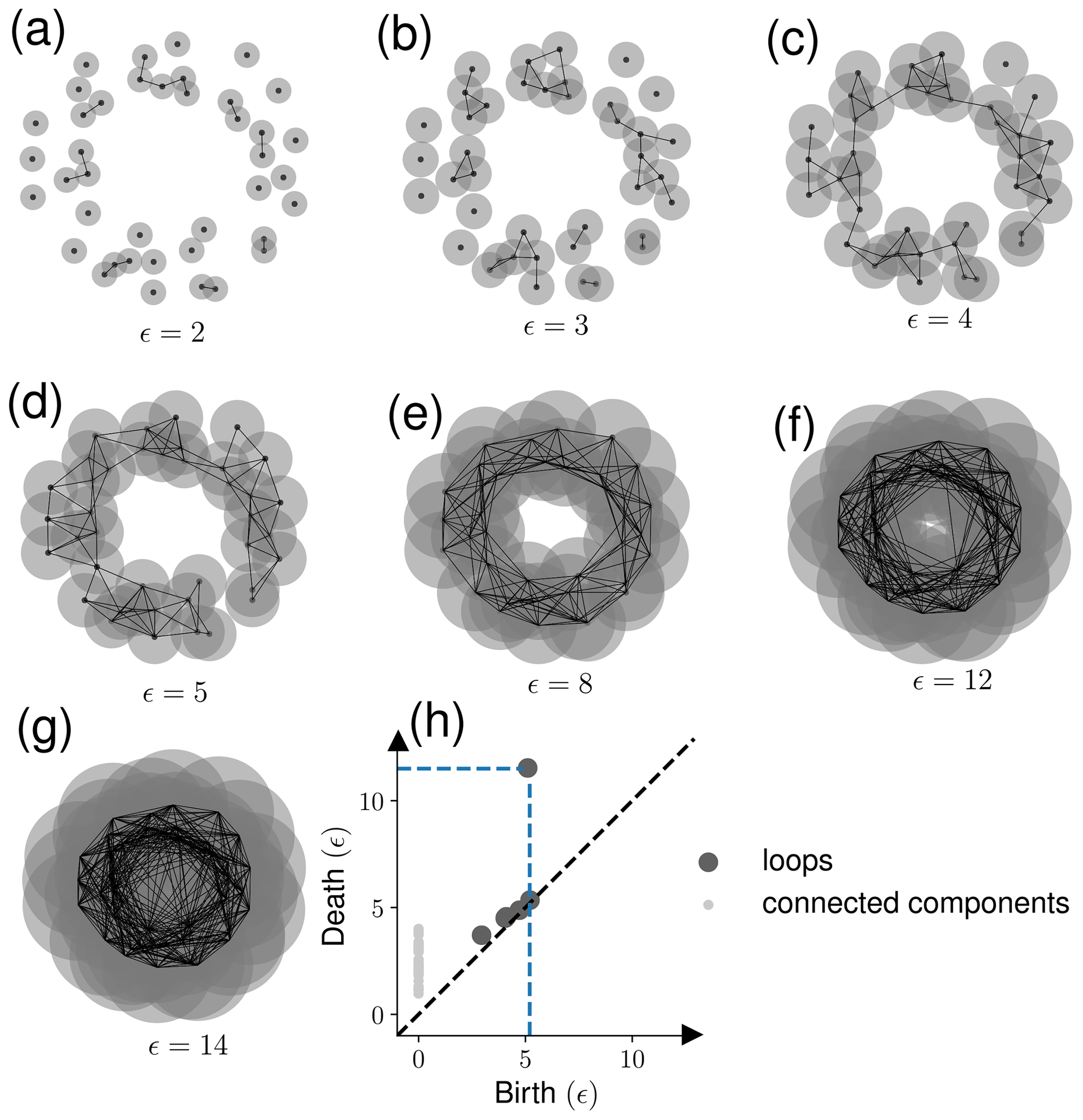
Figure 4 An example of using persistence homology: the data points are sampled from a noisy circle. (a–g) As the disk's radius increases ($\frac{\mathit{ϵ}}{\mathrm{2}}$), persistence homology captures various structures in the data. (h) The origin (birth) and disappearance (death) of loops and connected components is shown in the persistence diagram. The biggest loop in the noisy circle data is captured by the data points shown with the blue dotted line in panel (h).

Generally, in TDA, one constructs a simplicial complex by the Vietoris–Rips complex method, where one chooses a parameter ϵ>0 to find the structure present in the data. For each pair of points (x, y) in the point cloud data, add an edge between x and y if the Euclidean distance (d) between x and y is less than ϵ. For an n-dimensional simplex, the distance between each pair of n+1 affinely independent points should be less than $\mathit{ϵ}\left(d\right(x,y)<\mathit{ϵ}$). Each value of ϵ provides a set of simplexes representing a data structure. Different values of ϵ could lead to a different structure in data. To get the complete information about the structures present in the data, all the possible values of ϵ are used, creating a sequence of simplicial complex (this process is called filtration, Fig. 4a–g).

Homology measures particular structures present in the data providing valuable information about the geometrical and topological properties of the data. For example, zero-dimensional homology captures connected components or clusters, one-dimensional homology measures loops, and two-dimensional homology measures voids (Munch, 2017; Hensel et al., 2021). Structures like connected components, holes, and voids originate (birth) and disappear (death) with a change in the value of ϵ. A persistence diagram, shown in Fig. 4h, documents the birth and death information of these structures. Using the birth and death information of clusters, holes, and voids present in the persistence diagram, we can calculate several topological features of the data. We used various topological features to quantify the shape of data such as persistence entropy, average lifetime, number of points, Betti-curve-based measure, persistence-landscape-curve-based measure, Wasserstein amplitude, bottleneck amplitude, heat-kernel-based measure, and landscape-image-based measure. Each topological metric considers different homology dimensions separately.

The above-mentioned topological features can be explained using two objects – one the set of the $\mathit{\left\{}\right(b_i,d_i){\mathit{\}}}_{i=\mathrm{1}}^{i=N}$ birth–death pair in the persistence diagram, where i and N are the birth–death pair index and the total number of birth–death pairs respectively, and two the elements of the lifetime vector $[l_i{]}_{i=\mathrm{1}}^{i=N}$, calculated as difference between death and life of the (b_i, d_i) pair ($l_i=d_i-b_i$). Then the number of points is the length of the lifetime vector, whereas Wasserstein and bottleneck amplitudes are the p-norm and ∞-norm of the lifetime vector, respectively. Average lifetime and persistence entropy are the average and Shannon entropy of the lifetime vector.

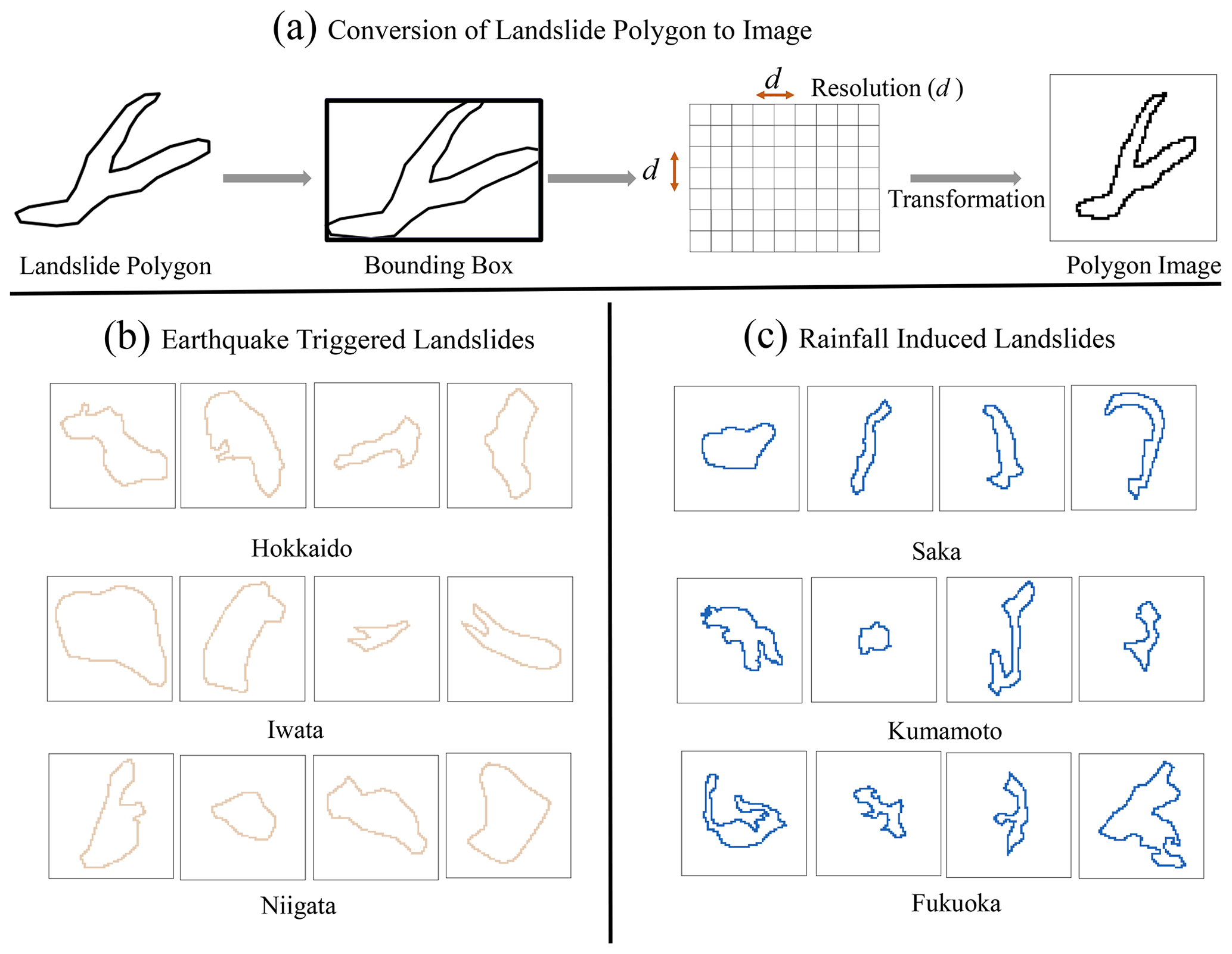
Figure 5 Sample input images for the image-based classification. (a) Flowchart of converting landslide planforms to a landslide polygon image. (b) Earthquake-triggered landslide image samples. (c) Rainfall-induced landslide image samples.

Betti- and persistence-landscape-curve-based features are calculated from the p-norm of discretized Betti and persistence landscape curves. The Betti curve is a function B(ϵ) that maps persistence diagram to an integer-valued curve, $B\left(\mathit{ϵ}\right):\mathbb{R}\to \mathbb{Z}$; it counts the number of (birth, death) pairs at ϵ that satisfy the condition $b_i<\mathit{ϵ}<d_i$ (Garin and Tauzin, 2019), whereas persistence landscape curve is a function $\mathit{\lambda }(k,\mathit{ϵ}):\mathbb{R}\to {\mathbb{R}}_{+}$, where $\mathit{\lambda }(k,\mathit{ϵ})=k_{\max }{\left\{f_{b_i,d_i}\left(\mathit{ϵ}\right)\right\}}_{i=\mathrm{1}}^{i=n}$, and k_max is the kth largest value of the set of functions defined by $f_{b_i,d_i}\left(\mathit{ϵ}\right)=\max \left\{\mathrm{0},\min \left(\mathit{ϵ}-b_i,d_i-\mathit{ϵ}\right)\right\}$ for each (b_i, d_i) pair (Bubenik and Dłotko, 2017).

The heat-kernel-based feature is calculated using the p-norm of the 2D function discretization obtained using the heat kernel on the persistence diagram. The heat kernel transforms the persistence diagram into a function of ℝ² obtained by placing a Gaussian kernel with standard deviation σ for each (birth, death) pair and negative of Gaussian kernel with the same standard deviation in the mirror image of (birth, death) pairs across the diagonal (Reininghaus et al., 2015), whereas the persistence-image-based measure is calculated using the p-norm of 2D function discretization obtained using the weighted Gaussian kernel on the birth-persistence diagram. The weighted Gaussian kernel transforms the birth-persistence diagram into a function of ℝ² obtained by placing a weighted Gaussian kernel with standard deviation σ for each (birth, death minus birth) pair in the birth-persistence diagram (Adams et al., 2017). In the birth-persistence diagram, the y axis represents the lifetime (death–birth) information of each (birth, death) pair.

3.3 Third method: image-based classification

In the third method, we used landslide planform images as input to convolutional neural networks (CNN) for the classification. We converted landslide polygons into binary images in a way that preserves the relative shape and structure of the polygons (Fig. 5). Then, using CNN for landslide trigger classification is straightforward via a simple CNN architecture with three convolutional layers and two fully connected layers. The input to CNN is a 64×64 binary pixel image, and the output is the probability of the input image belonging to one of the landslide trigger classes.

Convolutional neural networks (CNNs) are a class of artificial neural networks that are effective for various applications, such as image classification and object detection (Li et al., 2014; Guo et al., 2017; Albawi et al., 2017). The CNN architecture for classification problems consists of the input, hidden, and output layers (as shown in Fig. 6). The input layer consists of the input data to CNN, an image of a landslide polygon in our application. The hidden layer primarily contains convolutional layers, max-pooling layers, and fully connected layers. Finally, the output layer provides the probability of input data belonging to an output class – rainfall-induced or coseismic.

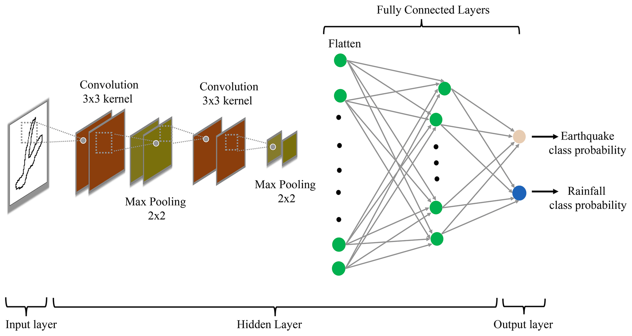
Figure 6 The figure shows the convolutional neural network (CNN) architecture used in the image-based method. The input of CNN is a binary-scale landslide image, and the output of CNN is the probability of a landslide image belonging to an earthquake- or rainfall-induced class.

Convolutional layers are the fundamental component of CNN that uses kernels (matrix of learnable parameters) to perform convolutions operations on the input. The resulting output of the convolution operation is called a feature map that learns the feature representation of the input data (Yamashita et al., 2018). Each neuron in a feature map captures the antecedent layer's local characteristics by convolution of kernels with the previous layer's feature maps (Guo et al., 2017). However, increasing convolutional layers could lead to over-parametrization and increase model complexity and, thus, overfitting. One of the ways to avoid the issue is to use pooling layers that reduce the feature map dimension and the number of neurons in the output layer of CNNs (Yamashita et al., 2018; Guo et al., 2017). We used max-pooling layers of n×n (n=2) size that take a patch of size n×n from a feature map and produce one value corresponding to that patch, and the pooling layer itself is free from parameters (Li et al., 2014).

Activation functions in CNNs capture the non-linear relationship between the input data and their output class. We used rectified linear unit (ReLU) activation for the hidden layer neuron activation functions as past studies have proved that ReLU activation improves classification results and learning speed (Li et al., 2014; Krizhevsky et al., 2012). The output of the ReLU activation function is $f\left(x\right)=\max (\mathrm{0},x)$; here x means the output of a neuron (Li et al., 2014). For the output layer, we used the softmax activation function. The softmax activation function calculates the output probabilities of the input sample belonging to each class in the last layer of CNN. The class probabilities are calculated as

$$\begin{array}{}\text{(1)}& P_i={\displaystyle \frac{\exp z_i}{\sum _{j=\mathrm{1}}^{j=m}\exp z_j}},\end{array}$$

where z_i is the output from the last layer of CNN corresponding to i class and m is the number of classes (in our case, m=2).

Fully connected (FC) layers work as a classification layer for CNNs, which comes after the convolutional layers. All layers in FC layers are fully connected, which means each neuron in a layer is connected to every neuron in the next layer of FC layers (Albawi et al., 2017; Guo et al., 2017). In classification problems, the last layer of the FC layer gives the probabilities of the input image belonging to one of the output classes with the help of the softmax activation function (Eq. 1). The output predicted probabilities of the input sample are used in a loss function that evaluates how well the model works for classifying the class of the input image data set. We used the cross-entropy loss function that measures the difference between actual and predicted probability distribution. The cross-entropy loss function for a sample is defined as $-\sum _{i=\mathrm{1}}^{i=m}{y}_i\log \left(\widehat{y_i}\right)$, where m is the total number of classes, and $y_i(\widehat{y_i}$) is actual (predicted) probability corresponding to class i. If i is the actual class of the input sample, then y_i=1; otherwise, y_i=0. In the case of binary classification, m=2. The sample's output probabilities are a function of parameters used in convolution kernels and FC layers to connect neurons in one layer to the next layer. These parameters are altered iteratively using the back-propagation algorithm and stochastic gradient method to increase the probability of samples belonging to the actual class and, thus, minimize the loss (Aurisano et al., 2016).

4 Landsifier model evaluation

We used two different testing configurations to evaluate the efficacy of our methods. Finding the triggers of individual landslides irrespective of their inventories is the first testing configuration. Here, we combined all the known trigger landslides from all six known triggered inventories and then split the combined landslide data into various training and testing sets following the k-fold cross-validation framework. In this testing configuration, landslides in each training and testing set are from all six landslide inventories. The second testing configuration finds the trigger of landslide inventories itself. We used all the possible combinations to train the algorithm on five known trigger inventories and test it on the sixth inventory. In this second testing configuration, landslides in the testing set are from a single inventory. Note that there are seven inventories in the analyzed data set, and six have known triggers. The analysis of this seventh inventory (Kumamoto unspecified) with unknown triggers is presented in Sect. 6.

4.1 Evaluation of the first method (geometric-feature-based classification)

Combining all the landslide inventories with known triggers leads to 26 501 samples (n_total), out of which 16 196 are earthquake-triggered landslides (n_earthquake) and 10 305 are rainfall-induced landslides (n_rainfall). As the number of earthquake-triggered landslides is much larger than the number of rainfall-induced landslides, we use equal numbers of each trigger class to avoid any class imbalance problems. To avoid selection bias and overfitting, we apply 10-fold cross-validation. k-fold cross-validation splits the combined classes data set into k random subsets where each iteration of cross-validation k−1 folds is used for training and the remaining fold for testing. We use 20 610 samples ($n_{\mathrm{rainfall}}=n_{\mathrm{earthquake}}=\mathrm{10}\mathrm{305}$) for cross-validation, and to get generalizable results we employ 1000 runs of cross-validation. In each run of cross-validation we randomly select 10 305 earthquake samples from 16 196 earthquake landslides. We achieved an 86.15±0.22 % classification accuracy for earthquakes, 85.29±0.19 % for rainfall, and 85.73±0.16 % as the mean classification accuracy.

For the second split configuration, we trained the random forest classifier on five inventories and tested it on the sixth inventory. For earthquake-triggered inventories the method achieved a classification accuracy of 66.62±0.65 %, 75.59±0.34 %, and 85.22±0.20 % for the Hokkaido (n_train=20 610, n_test=3256), Iwata (n_train=20 610, n_test=4160), and Niigata (n_train=14 832, n_test=8780) inventories (for geographical locations of these inventories see Fig. 1). For rainfall-induced inventories, we achieved a classification accuracy of 83.63±0.41 %, 69.40±0.61 %, and 92.12±0.25 % for the Kumamoto (n_train=9482, n_test=5564), Fukuoka (n_train=16 762, n_test=1924), and Saka (n_train=14 946, n_test=2817) region. In each one of the cases, we took an equal number of earthquake- and rainfall-triggered landslide samples to avoid any class imbalance issues (n_earthquake=n_rainfall). The low standard deviation in classification accuracy shows that results are stable with a change in training samples.

4.2 Evaluation of the second method (topological-feature-based classification)

In the first test and training set split configuration, as in Sect. 4.1, we used n_total=20 610 (total number of samples), n_earthquake=10 305 (number of earthquake-triggered samples), and n_rainfall=10 305 (number of rainfall-induced samples), keeping numbers of each trigger class equal to avoid class imbalance. We first identify the top 10 relevant topological features out of thirty features, employing 1000 runs of 10-fold cross-validation of random forest. Using these top 10 relevant topological features as the feature space for the random forest classifier, we carry out 1000 runs of 10-fold cross-validation to get the generalized classification accuracy. The method achieved an above 94 % classification accuracy for earthquake, rainfall, and mean class classification.

In the second split configuration, this method achieves an above 90 % accuracy for the Iwata, Niigata, Kumamoto, and Saka inventories. For the Hokkaido and Fukuoka region, the method achieves an above 80 % classification accuracy (see Fig. 7). The number of training and testing samples for each case is the same as in Sect. 4.1.

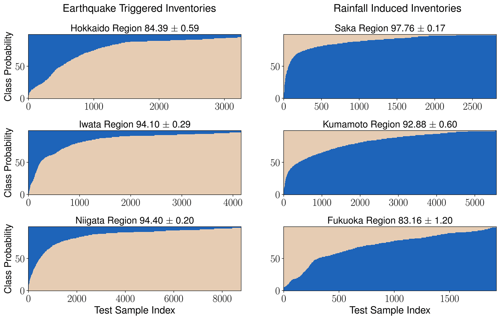
Figure 7 The topological-feature-based method (second method) accuracies for all the six known triggered inventories. The model is trained on five inventories in each case and tested on the sixth inventory. The y axis in the plot shows the probability of landslides belonging to the earthquake and rainfall class, and the x axis shows the sample index of landslides.

4.3 Evaluation of the third method (image-based classification)

As explained above in Sect. 3.3 we removed large landslides from the analysis, leading to n_total=24 311, n_earthquake=14 892, and n_rainfall=9419. We used an equal number of training samples of the coseismic and rainfall-induced landslides to avoid any class imbalance issues. We used 100 runs of different test and training sets instead of different runs of 10-fold cross-validation as convolutional neural networks are computationally expensive. The method achieved an above 85 % classification accuracy for earthquake, rainfall, and mean class classification.

For the second split configuration, the method achieved an above 80 % accuracy for the Saka region (n_train=13 738, n_test=2550). For the Niigata (n_train=12 780, n_test=8502), Kumamoto (n_train=8276, n_test=5281), and Fukuoka (n_train=15 662, n_test=1588) region, the method achieves an accuracy of above 70 %. The method achieves a 67 % accuracy for the Hokkaido inventory (n_train=18 838, n_test=2431). In each one of the cases, we took an equal number of earthquake- and rainfall-induced landslide samples to avoid class imbalance issues.

5 Landsifier library

One of the main aims of this paper is to introduce Landsifier, a Python library we built to provide the landslide research community with a user-friendly computational package to implement the methods described above. At the moment, we have made the code available on the corresponding author's GitHub: https://github.com/kamalrana7843/Landsifier.git (last access: 17 November 2022). Furthermore, we published the Landsifier library under an open-source license so that it is accessible via the Python terminal using the import command. In Sect. S2 we provide details of the library and brief descriptions of the available functionalities. Apart from three different methods for landslide trigger classification, the library also contains other useful functions like calculating geometric properties of landslide polygons, converting polygons to binary-scale images, downloading DEMs corresponding to an inventory region, and converting the 2D landslide polygon to a 3D landslide shape (see Figs. 3a and 5a). Please refer to Sect. S2 for further details about the library functions (Fig. S1 in the Supplement). Each of the three methods used in the library is simple to use and only requires polygon shapefiles as input. Also, the computation process is relatively fast; for example, the geometric, image, and topological-feature-based method takes less than 5, 15, and 45 min for training on 20 000 landslides (equal earthquake and rainfall samples) on a windows machine with 16 GB of RAM (random-access memory) using only landslide shapefiles as input. Moreover, none of the methods requires a GPU (graphics processing unit).

6 Discussion

The geometric properties of landslides can provide information about their trigger (Taylor et al., 2018). Our preliminary work on landslide trigger classification demonstrated that landslides with identical triggers share similar geometric properties, which could be exploited to classify landslide triggers – see the publication Rana et al. (2021) and briefly reproduced results here in Sects. 3.1, 4.1, and S1. In this work, we further expanded our initial approach by adding two additional methods for landslide trigger classification and a Python library Landsifier to implement them. One of these two new methods uses 3D shapes of landslides for their trigger classification by incorporating the elevation information. We compute topological features of these 3D shapes using topological data analysis (TDA) and use the features as an input to a machine-learning-based algorithm – random forest. The other method uses binary-scale landslide polygon images as an input to convolutional neural networks (CNNs) for the classification. Using six landslide inventories spread over the Japanese archipelago, we showed that each method exhibits strong performance in classifying landslide triggers. However, each method has its strengths and limitations that primarily depend on training and testing landslide data quality, quantity, and location. We explained each method's strengths and limitations in different conditions in this section. Before providing some hints about potential future work and opportunities that could arise from using Landsifier library, here, we also present and discuss the results of each of the three methods on the seventh Kumamoto unspecified inventory.

The landslide data quality depends on the data-acquiring technique; e.g., landslide data obtained using aerial or satellite images are much higher quality than the data acquired via field campaigns. Geologists collect landslide data acquired via field campaigns, and, naturally, such inventories tend to fail to represent the smaller landslides and cover the larger landslides (Ozturk et al., 2020), whereas landslide inventories acquired via aerial or satellite images cover both small and larger landslides and are called complete inventories as they adequately capture landslides of various sizes in their respective study area; e.g., see Schmitt et al. (2017). The performance of developed methods depends on landslide data quality, and without similar data quality in the training and testing set the accuracy of classification techniques could be insufficient to conclude the trigger of landslide inventory and also might lead to biases. Training the geometric-feature-based and image-based methods on landslide planforms with landslide data acquired via satellite or aerial images and testing on data acquired via field campaign or vice versa could lead to biases in landslide classification results. The methods based on landslide planform shape consider the area and perimeter as the most important features and rely on the information that coseismic landslides are generally larger than rainfall-induced landslides (Rana et al., 2021) (e.g., Taylor et al., 2018; Tanyaş et al., 2022). Therefore, a testing inventory triggered by rainfall but which lacks smaller landslides due to the field campaign acquisition technique could be classified as earthquake-triggered – given that training inventories are satellite- or aerial-image-based. We recommend using similar field-campaign-acquired inventories with known triggers to train the models for more accurate classification in such a scenario. Another option is to sample landslides from the satellite- or aerial-image-based inventories that resemble the size distribution of the testing data acquired via field campaign. This shortcoming motivated us to offer another alternative solution relying on topological analysis of 3D shapes of landslides.

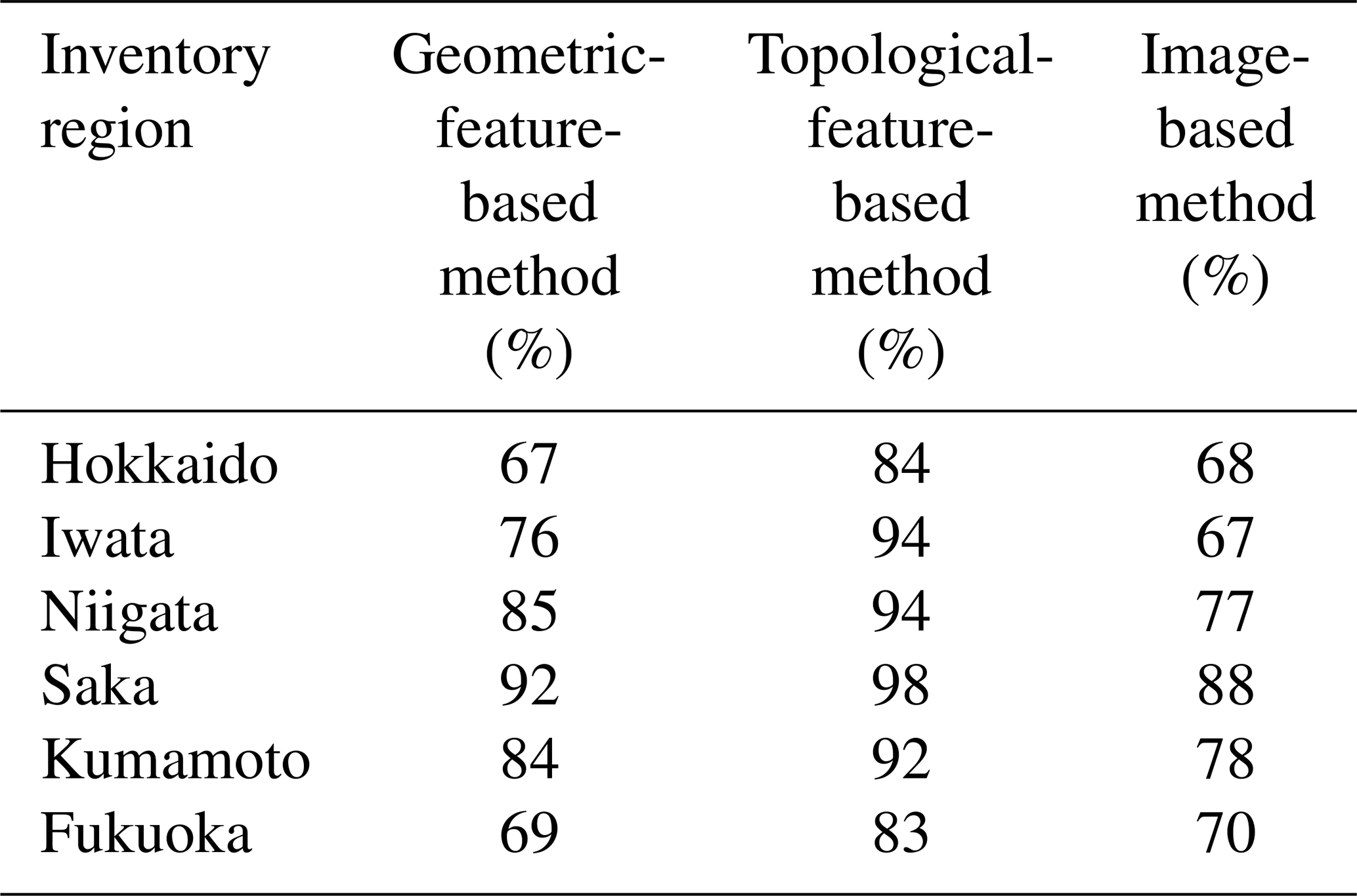
Landslides are 3D shapes; thus, using 3D shapes of landslides instead of 2D could provide additional information related to the landslide morphology. Consequently, a 3D-landslide-shape-based method might elevate classification accuracy, especially in regions without proper training and testing data of similar quality. We use TDA, a method rooted in algebraic topology, to compute topological features of a landslide's 3D shapes to classify landslide triggers. The TDA-based method extracts topological information along with geometric information of landslide shape, whereas the geometric-feature-based method and likely the image-based method use only geometric information of the landslide shape for landslide classification. We expect the TDA-based method will provide best landslide trigger classification results. In Table 1 one can observe that the TDA-based method indeed performs better than the other two methods. However, TDA-based measures encode landslide morphology; hence, if testing and training inventories share similarities in the geomorphology of the studied regions (spatial autocorrelation) (Oksanen and Sarjakoski, 2005), then the trigger prediction is highly influenced by training inventory. Geometric-feature- and image-based methods are less sensitive to the geomorphological similarities between the training and testing landslide inventories, as these only use the 2D landslide planforms. However, the image-based method performs satisfactorily only when an adequate number of training data are available. Hence, we recommend using geometric- or topological-feature-based methods in inventories with limited landslide counts.

Table 1 The table shows landslide classification results using the three methods. The model is evaluated on all possible training set combinations of the five inventories and tested on the sixth inventory.

We applied each method to classify landslides triggers in the Kumamoto unspecified inventory having an undocumented trigger to demonstrate the real-world application of the Landsifier library. Out of 612 landslides in the inventory, the geometric-feature-based method and topological-feature-based method classified 604 and 612 landslides as earthquake-triggered. In comparison, the image-based method uses 164 landslides after removing landslides having width and length greater than 180 m (see Sect. 3.3 for more details) and classified all of the landslides as seismically triggered. As each method classifies the majority of the landslides as earthquake-triggered, we are confident that earthquakes are the most likely trigger for most of the landslides in this inventory. Moreover, the Kumamoto unspecified inventory documents landslides along the rims of the Aso Caldera, and the active volcano Mount Aso shakes the surrounding area frequently, triggering landslides within its vicinity (Saito et al., 2018). Hence, it is very likely that this inventory consists of landslides of coseismic origin.

Considering the above discussions, in future work, we plan to explore further the sensitivity of our trigger classification methods to spatial autocorrelations. We will also examine the influences of landslide size distributions on each method. Specifically, we plan to classify the trigger of large landslides (area > 90 000 m²), as they are the most dangerous landslides and affect a huge area, by training each method on a large-landslide-training dataset. Moreover, we will consider model transferability to different regions by extensively testing these methods on national landslide inventories, e.g., India, Nepal, Taiwan, and the USA. Our methods could also provide other opportunities – for example, assessing landslide-prone regions as an alternative to landslide susceptibility measure using TDA. Also, TDA could be used to classify landslide types, according to the types described in Cruden and Varnes (1996) and Varnes (1978). Landslide type information plays a crucial role in landslide risk assessment, which is usually missed in landslide databases (Loche et al., 2022). We plan to further develop the current version of the Landsifier by incorporating a landslide type classifier in the next version (e.g., Amato et al., 2021). This method will be able to find the analogy between an observed landslide type and a generic landslide type following Cruden and Varnes (1996).

7 Conclusions

The landslide-triggering mechanism is crucial information to develop landslide hazard models; e.g., a landslide hazard model for extreme rainfall incidents requires landslide inventories related to rainfall events only. However, modern automated landslide mappers for continuous monitoring and historical landslide inventories rarely report the landslide-triggering mechanism. Missing triggers in the landslide inventories decrease their efficacy for landslide hazard models. In this work, we developed a Python library, Landsifier, containing three methods for landslide trigger classification by exploiting landslide planforms and 3D shapes. To develop the first two of these methods, we combined geometric and topological features with machine learning, and in the third method, we used deep learning. The latter two methods are new; i.e., we are reporting them here for the first time.

We use seven landslide inventories spread over the Japanese archipelago. Six of these seven inventories have known triggers, while the seventh inventory has a missing trigger. We applied each method to all possible sets of five training inventories and one testing inventory using six known triggered inventories. Moreover, we took different training and testing sets of landslides by mixing all known triggered landslide inventories following the k-fold cross-validation. The achieved results demonstrate that the methods are robust and capable of classifying triggers of landslide inventories with high accuracy (70 %–95 %). To demonstrate the real-world application of our toolbox, we also applied the three methods to the seventh inventory without any triggering information and classified it as an earthquake-triggered inventory.

The Python-based Landsifier library provides a user-friendly computational package to implement the methods described above to the landslide research community. Two of the three methods included in the library are new and introduced here for the first time, while the third method is published in our previous work. To the best of our knowledge, Landsifier is the first Python tool developed for landslide trigger classification, and also such a tool does not exist in other programming languages. We anticipate that the landslide research community will find the Landsifier library helpful in finding the trigger mechanism of inventories or individual landslides. The presented methods and the library could be deployed in any region of the world with adequate training data from areas with similar climatic and tectonic features. The Landsifier library also contains useful functions like finding geometric properties of landslides polygons, downloading DEMs corresponding to an inventory region, and converting landslide polygons to landslide 3D shapes; these elements could be useful for the landslide research community.

Furthermore, methods in the Landsifier library are easy to use as they require only shapefiles of landslide polygons as input. Landsifier is a modular software; we hope the landslide community will further improve the offered tool and expand the available functions for new applications such as classifying landslide types, assessing landslide-prone regions, and other possible uses listed in the discussion section. At the moment, we have made the code available on the corresponding author's GitHub: https://github.com/kamalrana7843/Landsifier.git (last access: 17 November 2022). Moreover, we published the Landsifier library under an open-source license so that it is accessible via the Python terminal using the import command. In Sect. S2, we provide details of the library and brief descriptions of the available functionalities.