Temporal changes in rainfall intensity–duration thresholds for post-wildfire flash floods in southern California

Rainfall intensity–duration (ID) thresholds are commonly used to assess flash flood potential downstream of burned watersheds. High-intensity and/or long-duration rainfall is required to generate flash floods as landscapes recover from fire, but there is little guidance on how thresholds change as a function of time since fire. Here, we force a hydrological model with radar-derived precipitation to estimate ID thresholds for post-fire flash floods in a 41.5 km² watershed in southern California, USA. Prior work in this study area constrains temporal changes in hydrological model parameters, allowing us to estimate temporal changes in ID thresholds. The results indicate that ID thresholds increase by more than a factor of 2 from post-fire year 1 to post-fire year 5. Thresholds based on averaging rainfall intensity over durations of 15–60 min perform better than those that average rainfall intensity over shorter time intervals. Moreover, thresholds based on the 75th percentile of radar-derived rainfall intensity over the watershed perform better than thresholds based on the 25th or 50th percentile of rainfall intensity. Results demonstrate how hydrological models can be used to estimate changes in ID thresholds following disturbance and provide guidance on the rainfall metrics that are best suited for predicting post-fire flash floods.

1 Introduction

Heightened hydrological responses are common within and downstream of recently burned areas, resulting in an increased likelihood of flash floods. Rainfall intensity–duration (ID) thresholds are commonly used to assess the potential for flash floods (Moody and Martin, 2001; Cannon et al., 2008). Many past studies aimed at defining thresholds for flash floods focus on the first 1–2 years following fires (Cannon et al., 2008; Wilson et al., 2018). Since the hydrologic impacts of fire are transient, rainfall ID thresholds associated with flash floods are likely to change as a watershed recovers (Ebel and Martin, 2017; Ebel and Moody, 2017; Moreno et al., 2020; Ebel, 2020). It may take more than a decade for hydrological responses to return to pre-fire levels, yet there is limited guidance on how the magnitude and utility of rainfall ID thresholds change with time since fire. Given the increased frequency and size of fires in many geographic and ecological zones (e.g. Gillett et al., 2004; Westerling et al., 2006; Kitzberger et al., 2017), it is of growing importance to quantify the best metrics for assessing flash-flood potential in the immediate aftermath of fire as well as how these metrics change throughout the recovery process (e.g. Ebel, 2020).

Rainfall ID thresholds for flash floods are typically defined using historic data that relate rainfall over different intensities and durations to an observed hydrological response, namely the presence or absence of flooding (e.g. Cannon et al., 2008). Due to the stochastic nature of rainfall over burned areas and limited observations throughout the recovery process, there is a paucity of data that can be used to derive empirical thresholds for flash flooding beyond 1 year of recovery. Hazards associated with flash flooding, however, may exist downstream of burned areas well beyond 1 year of recovery. Wildfires alter rainfall-runoff partitioning and flood routing by incinerating vegetation and reducing interception capacity (Stoof et al., 2012; Saksa et al., 2020), decreasing hydraulic roughness, and reducing soil infiltration capacity (Larsen et al., 2009; Ebel and Moody, 2013). Reductions in infiltration capacity are often attributed to fire-induced soil-water repellency (Ebel and Moody, 2013), which is generally strongest immediately following a fire and then decays over timescales ranging from 1 year to more than 5 years (Dyrness, 1976; Huffman et al., 2001; Larsen et al., 2009), though surface soil sealing (Larsen et al., 2009) and hyper-dry conditions (Moody and Ebel, 2012) are also known to play important roles. Vegetation recovery, which may influence temporal changes in hydraulic roughness and canopy interception, can take 5 years or longer. Cannon et al. (2008) collected sufficient data over a 2-year time period following fires in southern California, USA, to define separate rainfall ID thresholds for post-fire debris flows and flash floods in the first and second years following fires. They found that the ID thresholds for flash floods and debris flows may increase by as much as 25 mm h⁻¹ after 1 year of recovery, a change that they attributed to a combination of vegetation growth and sediment removal as a result of rainstorms during the first post-fire year.

Rainfall ID thresholds are often defined over a range of durations, though averaging rainfall intensity over a particular duration may provide a more reliable threshold. The post-fire hydrological response in the first few years is often best related to rainfall intensity over short durations (less than 60 min) (Staley et al., 2017; Moody and Martin, 2001). In their efforts to define rainfall ID thresholds for post-fire debris flows, Staley et al. (2013) showed that averaging rainfall intensities over durations between 15 and 60 min resulted in thresholds that performed better relative to those associated with longer durations. One potential explanation for this observation is that post-fire debris flows are often triggered by runoff in steep, low-order drainages, which both Kean et al. (2011) and Raymond et al. (2020) have found to be highly correlated with rainfall intensities averaged over similarly short time intervals (10–15 min). Moody and Martin (2001) have also documented a substantial increase in peak discharge following wildfires once the 30 min rainfall intensity (I₃₀) crossed a threshold value, suggesting that I₃₀ may be a consistent predictor of flash flood activity in recently burned watersheds. Moody and Martin (2001) suggest that peak I₃₀ can be used to set the threshold for early warning flood systems. The optimal duration for defining post-fire flash floods thresholds, as well as how it may change with time, remains relatively unexplored.

Rain gage records are typically used to derive rainfall ID thresholds for flash flood and post-fires debris flows (Staley et al., 2013, 2017). Post-fire debris flows, however, tend to initiate in small (<1 km²), steep watersheds. In these small watersheds, the rainfall intensity responsible for initiating a debris flow can be characterized by a single rain gage installed near the initiation zone. Flash floods differ in that they tend to occur at larger spatial scales where rainfall is spatially variable and may not be adequately characterized by data from a single rain gage. Radar-derived precipitation estimates, which can provide high spatiotemporal rainfall intensity resolution, present opportunities to develop basin-specific thresholds for post-fire flash floods. However, high spatiotemporal variability in rainfall intensity also brings new challenges when employing radar-derived precipitation in flood warning practice. In particular, what is the best way to summarize spatially and temporally variable rainfall intensity information with a single metric that can be used as a threshold? How does hydrological recovery following fires influence the generation of flash floods and the metrics that are best suited for their prediction? Data-driven approaches to answering these and related questions may be hampered by limited monitoring of post-fire hydrological response throughout the recovery period and the stochastic occurrence of rainfall over burned areas, which limits opportunities for observations. Given a well-constrained hydrological model that accounts for changes associated with post-fire recovery, it is possible to use numerical experiments to understand relationships between time since fire, the spatiotemporal patterns of rainfall over a watershed, and the occurrence of flash floods.

Figure 1 Modified from Fig. 1 in Liu et al. (2021) (a) The location of the upper Arroyo Seco watershed within California. The red triangle indicates the location of the USGS stream gage (11098000); (b) Shaded relief showing the study watershed with the USGS stream gage (red triangle; 34^∘13^′20^′′, −118^∘10^′36^′′); (c) Soil burn severity for the 2009 Station fire. Burn severity percentages are for planform area within each category.

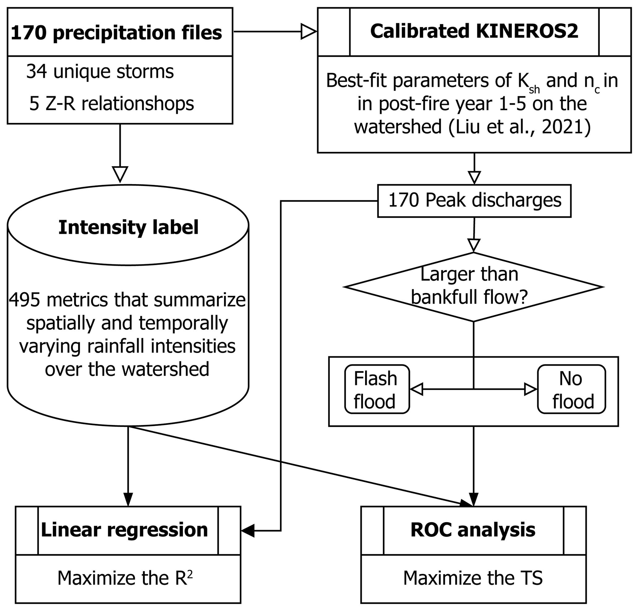
Here, we use observed patterns of spatially and temporally varying radar-derived rainfall estimates over a 41.5 km² watershed in the San Gabriel Mountains of southern California, USA, to (1) determine the optimal method to define a rainfall ID threshold for flash floods, and (2) identify changes in rainfall ID thresholds for flash floods as a function of time since fire. The watershed, which we refer to as the upper Arroyo Seco, burned during the 2009 Station Fire (USDA Forest Service, 2009). Liu et al. (2021) used rain and stream gage data collected at different times following the fire to calibrate the KINEROS2 hydrological model for this watershed, enabling them to quantify temporal changes in model parameters as a function of time since fire. Combining this calibrated model with spatially explicit, radar-derived estimates of rainfall intensity during 34 rainstorms, we explore the utility of different rainfall ID metrics as flash flood thresholds and quantify temporal changes in those thresholds through the first 5 years of recovery. Results provide insight into the magnitude of temporal changes in flash flood thresholds in the densely populated, fire-prone region of southern California. Findings also provide guidance for the magnitude of change expected in rainfall ID thresholds for flash floods during the post-fire recovery period in chaparral-dominated environments similar to southern California. More generally, results support the development of early warning systems for flash floods by identifying specific metrics that can be computed using spatially variable rainfall intensity estimates to assess the potential for flash flooding. The optimal rainfall ID metrics identified in this study could be helpful when issuing flash flood warnings based on radar-derived precipitation estimates or data from several real-time rain gages within a watershed.

2 Study area

The upper Arroyo Seco watershed drains the 41.5 km² area above USGS stream gage station (11098000) near Pasadena in the San Gabriel Mountains (Fig. 1). The upper Arroyo Seco was burned in the August–October 2009 Station Fire, which burned more than 80 % of the watershed at moderate-to-high soil burn severity (USDA Forest Service, 2009). Dominant shrubs and chaparral, such as chamise (Adenostoma fasciculatum) and manzanita (Arctostaphylos spp.), were completely consumed with severe soil heating in isolated patches throughout many areas burned at moderate-to-high severity (USDA Forest Service, 2009). Soils in this area are typically sand and silty–sand textured and thin (<1 m) with partial exposure of bedrock (Staley et al., 2014). The majority of rainfall in the study area typically occurs in the cool season, between December and March, while warm, dry conditions dominate from April to early November. The San Gabriel Mountains also experience some of the most frequent short-duration, high-intensity rainfall event in the state (Oakley et al., 2018a).

Due to wildfire-induced changes in surface conditions, including canopy cover and soil-hydraulic properties, runoff generation in the first year following the fire was likely dominated by infiltration excess overland flow (Schmidt et al., 2011; Liu et al., 2021). Enhanced soil-water repellency (SWR), which helps promote low infiltration capacity, and extensive dry ravel, which loads channels with fine-grained hillslope sediment, are both commonly observed after fires in the San Gabriel Mountains (e.g., Watson and Letey, 1970; Hubbert and Oriol, 2005; Lamb et al., 2011; Hubbert et al., 2012). Rengers et al. (2019) calibrated a hydrologic model using data from small watersheds (0.01–2 km²) burned by the Station Fire and found relatively low values for saturated hydraulic conductivity (K_s), generally between 2 and 10 mm h⁻¹. These results are consistent with values for saturated hydraulic conductivity inferred by Liu et al. (2021) via model calibration in the upper Arroyo Seco watershed. The impact of dry ravel, which reduces grain roughness in the channel network, and reduced vegetation density led to estimates of Manning's n in the channels of the upper Arroyo Seco of approximately 0.09 s m${}^{-\mathrm{1}/\mathrm{3}}$ in the first year following fires (Liu et al., 2021). These hydrologic changes led to widespread flooding and debris flows during multiple rainstorms in the first winter after the fire (Kean et al., 2011; Oakley et al., 2017). As hydrological recovery began over the next several years, the watershed-scale K_s and Manning's n generally increased and likely started to mitigate the flash flood risk (Liu et al., 2021).

3 Data and methods

3.1 Radar-derived precipitation

Weather radar coverage is adequate for estimating rainfall over the study area (NOAA, 2021a, b), and radars have been operational since the mid-1990s. This allows us to utilize observed data to capture temporal and spatial characteristics of storms impacting the study area, a region of complex terrain. We sought to identify storms in the study area that produced moderate-to-high intensity rainfall to use as inputs to a hydrological model to simulate flood responses. Storm events were selected within the period for which observations are archived for the two operational NWS Next-Generation Weather Radar installations (NEXRAD; NOAA, 1991) that cover the study area, KSOX (Santa Ana) and KVTX (Ventura). Archives for the radars begin in 1997 and 1995, respectively.

We compiled storm events starting with those known to have produced high intensity rainfall and a debris flow response in the San Gabriel Mountains (e.g., Table 1 in Oakley et al., 2017) as well as other storms that produced high-intensity rainfall in the region (e.g., Oakley et al., 2018b; Cannon et al., 2018). We then used hourly rainfall observations from the Clear Creek (2002–present), San Rafael Hills (2005–present), and Henninger Flats (2010–present) Remote Automated Weather Stations (RAWS, acquired from https://raws.dri.edu/, last access: 2 February 2022) as indicator gages for the study area. This further limited us to post-2002 events outside of the literature. All gages are <10 km from the watershed of interest; there were no long-record gages within the watershed. We used 15 mm h⁻¹ as a threshold for moderate-to-high intensity rainfall and extracted all events from the gage record meeting or exceeding this value to develop a list of events of interest. This threshold generally corresponds with a 1-year average recurrence interval storm event in the study area (NOAA, Atlas 14). This value falls between the California–Nevada River Forecast Center's flash flood guidance for unburned areas in the region (∼ 22–25 mm h⁻¹; CNRFC, 2022) and regional thresholds for post-wildfire debris flows in this region at a point (12.7 mm h⁻¹, Cannon et al., 2008; Staley et al., 2013). This threshold allows us to focus on storms that have a high potential to generate floods, while keeping the number of storms to a manageable level for data processing. We reviewed the radar data for these events, at which point some of the selected events could not be utilized due to radar outages or poor data quality. This exercise presented us with 34 storm events (Table S1 in the Supplement).

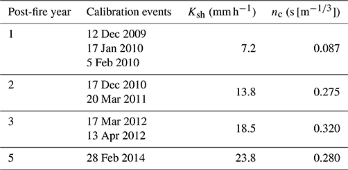
Table 1 Summary of model parameters for post-fire years 1, 2, 3, and 5. The saturated hydraulic conductivity on hillslopes (K_sh) and hydraulic roughness in channels (n_c) are the average of values calibrated in post-fire years 1, 2, 3, and 5 (Liu et al., 2021).

Various atmospheric processes may contribute to generation of moderate-to-high rainfall intensities (e.g., Oakley et al., 2017), resulting in differing spatial and temporal precipitation patterns over a burn area. To ensure the events selected captured the variability in spatial and temporal precipitation characteristics, we evaluated the spatial characteristics of the events. We found rainfall patterns could generally be categorized into four main spatial patterns at the scale of several tens of kilometers: (1) a broad pattern, with a contiguous area of moderate-to-high intensity precipitation (>45 dBZ) spanning tens of kilometers; (2) a scattered pattern with numerous cells of moderate-to-high precipitation that are not spatially continuous; (3) an isolated pattern, with one to a few isolated cells of moderate-to-high intensity rainfall separated by non-precipitating areas several to tens of kilometers in extent; (4) a narrow cold frontal rainband (NCFR) – a north–south oriented narrow band (∼ 3–5 km wide, tens to 100 km in length) of very high intensity rainfall (e.g., Oakley et al., 2018b; Cannon et al., 2020; Figure S1). At the <10 km horizontal scale (the scale of the watershed), it was harder to identify meaningful patterns and distinctions, though the larger-scale signals imply varying spatial and temporal patterns of precipitation as each pass over the watershed. A table of storm events and their characteristics is available in Table S1.

An approximate start and end time were determined for each event using the Clear Creek RAWS gauge as an indicator. Start time was determined by identifying the time of maximum 1 h rainfall in the event and going back in time to the first of three consecutive hours of >1.5 mm h⁻¹ precipitation. The end of an event was determined as the last hour where precipitation dropped below 3 mm h⁻¹ for at least two consecutive hours.

Level-II base reflectivity (https://www.ncdc.noaa.gov/wct/, last access: 2 February 2022) between the start and end time of each event was downloaded from both the KSOX and KVTX radars. The data were used to generate spatially distributed precipitation over the study area. Radar imagery concurrent with the gauge-based record of high intensity rainfall events was converted to a composite maximum reflectivity product at 250 m spatial and 5 min temporal resolution. Conversion of radar reflectivity to rain rate required the application of an empirically derived reflectivity (Z) to rain rate (R) relationship (e.g. Marshall and Palmer, 1948). The Z-R relationship is conventionally represented by the equation Z=aR^b, which includes parameters a and b to account for variations in precipitation for a given reflectivity arising from differences in the drop size distribution. Due to the lack of previous studies investigating Z-R relationships in precipitating conditions over the region of interest, there are no standard a and b parameters to apply to the reflectivity data analyzed here. Thus, five well-known and previously published Z-R relationships were applied to the gridded reflectivity values. Supplement S3 lists the different Z-R relationships applied here and the general conditions for which they are suitable. Although the Z-R relationships used here are not based on observations from the present study's region of interest, the variation of a and b parameters yields an estimate of precipitation uncertainty. It is worth noting that a number of additional sources of radar measurement uncertainty exist that are not evaluated in depth here, including beam broadening, topographic blocking, and scan elevation. However, this was not of primary concern since the goal of this study was to generate realistic spatial and temporal patterns of rainfall over the watershed with varying intensity that could be used to force the KINEROS2 hydrological model. The goal was not to reproduce the observed hydrological response resulting from a particular set of rainstorms.

As a range of precipitation intensities for each storm result from the application of the five different Z-R relationships (e.g., Fig. S2), we utilize these as plausible storms of varying precipitation intensity to increase our storm sample size, such that we apply 34 storms ⋅ 5 Z-R relations = 170 precipitation scenarios as inputs to KINEROS2. These 170 scenarios were then processed for ingestion into KINEROS2 (Fig. 2).

Figure 2 Delineation of rainfall intensity–duration threshold for post-fire flash flood.

3.2 Summary metrics for spatially and temporally varying rainfall

In search of a spatiotemporal summary metric that may serve as a reliable flash flood threshold, we begin by describing a methodology to summarize spatially and temporally varying rainfall over a watershed. For a given rainstorm, the rainfall intensity time series at a single point, such as a single radar pixel, can be summarized by computing a moving average of intensity over a specified duration, D. Letting t denote time and R denote the cumulative rainfall (mm), we define the rainfall intensity over a duration D at any given pixel within the watershed as

$$\begin{array}{}\text{(1)}& I_D\left(t\right)={\displaystyle \frac{R\left(t\right)-R(t-D)}{D}}.\end{array}$$

Here, we compute I_D(t) for each pixel for durations of 5, 10, 15, 30, and 60 min. Since the intensity in each radar pixel could have a unique value, we also need a way to summarize I_D(t) in space. One option would be to take the median of I_D(t) to determine a typical value of I_D within the watershed at each time, t. However, the median may not be a good predictor of flash flooding since one could envision a scenario where it is only raining over $\mathrm{1}/\mathrm{3}$ of the watershed, yet it is raining with sufficient intensity to generate a flash flood. We therefore compute the jth percentile of I_D(t) at each time, t, for j between 1 and 99. We denote the jth percentile of I_D(t) as $I_D^j\left(t\right)$. For each rainstorm, we focus our analysis on the peak value of $I_D^j\left(t\right)$ which we denote as $I_D^j$. As an example, $I_{\mathrm{30}}^{\mathrm{50}}$ would be computed by defining I₃₀ for all radar time steps within a rainstorm, determining the median value of I₃₀ over the watershed at each of those time steps, and then taking the maximum of that time series of median I₃₀ intensities. This analysis yields 495 different metrics ($I_D^j$ for $j=\mathrm{1},\mathrm{2},\mathrm{\dots },\mathrm{99}$ and $D=\mathrm{5},\mathrm{10},\mathrm{15},\mathrm{30},\mathrm{60}$) that summarize spatially and temporally varying rainfall intensities over the watershed. In the following sections, we describe how we test the utility of each of these 495 different metrics as a flash flood threshold. A threshold defined by $I_D^j$ would denote a threshold where (100–j)% of the watershed experiences rainfall of duration D with an intensity of I or greater.

3.3 Hydrological modeling

We used the KINEROS2 (K2) hydrological model to simulate the rainfall partitioning, overland flow generation, and flood routing in the upper Arroyo Seco watershed. K2 is an event-scale, distributed-parameter, process-based watershed model, which has been used extensively for rainfall-runoff processes in semi-arid and arid watersheds (Smith et al., 1995; Goodrich et al., 2012). Liu et al. (2021) used rain gage data in combination with the USGS stream gage installed at the outlet of the upper Arroyo Seco watershed to calibrate K2 during different stages of the post-fire recovery process. We use the same model setup for simulations in this study. In particular, the 41.5 km² watershed was discretized into 1289 hillslope planes and these planes were connected by a stream network of 519 channel segments based on a 1 m lidar-derived digital elevation model (DEM). After accounting for a fixed interception depth of 2.97 mm based on the land cover look-up table in the Automated Geospatial Watershed Assessment toolkit (AGWA; Miller et al., 2007), infiltration of rainfall into soil is represented using the Parlange et al. (1982) approximation. Overland flow and channel flow are modeled by kinematic wave equations. Both saturated hydraulic conductivity on hillslopes (K_sh) and hydraulic roughness in channels (n_c) primarily determine runoff generation and the shape of hydrograph, including total runoff volume, peak discharge rate, and time to peak (Canfield et al., 2005; Yatheendradas et al., 2008; Meles et al., 2019). Other parameters, such as hydraulic roughness (n_h) and capillary drive (G_h) on hillslopes, had a relatively minor impact on modeled runoff after the Station Fire in the upper Arroyo Seco watershed (Liu et al., 2021).

Liu et al. (2021) found that both K_sh and n_c were lowest immediately after the fire. K_sh increased, on average, by approximately 4 mm h⁻¹ yr⁻¹ during the first 5 years of recovery, whereas n_c increased by more than a factor of 2 after 1 year of recovery and then remained relatively constant. We focus here on simulating the response to rainfall in the first 5 years following the fire, when the watershed is likely most vulnerable to extreme responses. To represent the temporal changes in K_sh and n documented by Liu et al. (2021) following the fire, we used different values of K_sh and n_c for each post-fire year (i.e. post-fire years 1, 2, 3, and 5) based on the values calibrated by Liu et al. (2021) in post-fire years 1, 2, 3, and 5 (Table. 1). Liu et al. (2021) were unable to calibrate the necessary K2 parameters in post-fire year 4 so we do not perform any simulations to constrain flash flood thresholds in that year. Initial soil moisture is set to a volumetric soil-water content of 0.1, following Liu et al. (2021). Other parameters were also given the same values as the calibrated K2 model, including saturated hydraulic conductivity of channels (1 mm h⁻¹), net capillary drive of channels (5 mm), hydraulic roughness of hillslopes (0.1 s m${}^{-\mathrm{1}/\mathrm{3}})$, net capillary drive of hillslopes (50 mm), and soil porosity (0.4). With this model setup, we simulate the response to each of the 170 rainstorms for post-fire years 1, 2, 3, and 5.

3.4 Rainfall intensity–duration thresholds

Each K2 simulation results in a modeled hydrograph at the watershed outlet. As a first step towards defining a flash flood threshold, it is necessary to determine, based on the modeled time series of discharge, whether or not a flash flood would have occurred. We defined the flash flood level as the discharge required to exceed bankfull flow (Sweeney, 1992), which we assumed was equal to the 2-year flood (Leopold et al., 1964). To determine the discharge associated with the 2-year flood, we performed a flood frequency analysis using HEC-SSP v2.2 (Bartles et al., 2019) based on annual maximum records at the USGS stream gage station (11098000). The discharge associated with the 2-year flood at the stream gage station is 15.3 m³ s⁻¹, with a 95 % confidence interval of 12.3–19.2 m³ s⁻¹ (Fig. S3). A flash flood threshold by this definition can be viewed as conservative since it may only indicate the onset of minor flooding as water begins to spill out of the channel. Based on this definition, we then used two approaches to identify the rainfall ID threshold for flash floods (Fig. 2).

The first approach is based on a linear regression analysis that relates peak discharge with different rainfall ID metrics, namely $I_D^j$ for different values of j and D. Using simulations of 170 rainfall-runoff events in each post-fire year, it is possible to determine a relationship for peak discharge (Q) as a function of $I_D^j$. Then, the rainfall ID threshold can be found by determining the rainfall intensity at which the peak discharge exceeds the bankfull capacity. The simplest quantitative relation is a linear regression:

$$\begin{array}{}\text{(2)}& Q=m{I}_D^j+k,\end{array}$$

where Q is the peak discharge (m³ s⁻¹) of a simulated hydrograph at the outlet, $I_D^j$ denotes rainfall intensity (mm h⁻¹) for the rainstorm that produced the hydrograph, and m and k denote the slope and y intercept of the linear regression, respectively.

Considering the channel dimensions and resolution of the DEM used in the K2 model, we selected intensity–discharge ($I_D^j-Q$) pairs associated with a Q greater than 2 m³ s⁻¹. The flow depth associated with a Q less than 2 m³ s⁻¹ would be very small and any impact from such flow would be negligible. The parameters in the linear Eq. (1) with the maximum determination coefficient ($R_{\max }^{\mathrm{2}}$) were estimated using least-squares linear regression in the SciPy Python library for the selected $I_D^j-Q$ pairs. A total of 495 linear regressions were produced for each year because $I_D^j$ can take on 495 different values (five durations, 99 percentiles) for each rainstorm. For each post-fire year, we then identified the maximum R² value for each duration as a function of percentile from 1st to 99th (Fig. 3). The rainfall ID threshold for flash flooding in each year was found, for each duration, from the linear relation associated with the largest R² (Fig. 4).

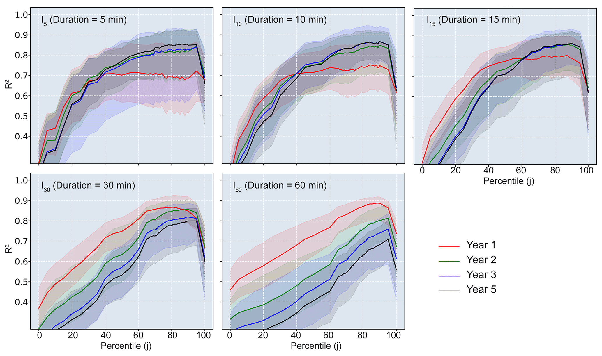
Figure 3 The determination coefficient (R²) and 95 % confidence interval associated with the linear regression between $I_D^j$ and peak discharge in post-fire years 1, 2, 3, and 5. Data used to fit the linear relation are from events with peak discharge greater than 2 m³ s⁻¹.

We also estimated the 95 % confidence interval (CI) of both R² and the rainfall ID threshold by performing bootstrapping resampling on 170 rainfall-runoff events for each year. The number of replications is 50. The 95 % CI was constructed with the 2.5 percentile and the 97.5 percentile of the ranked R² or rainfall ID threshold.

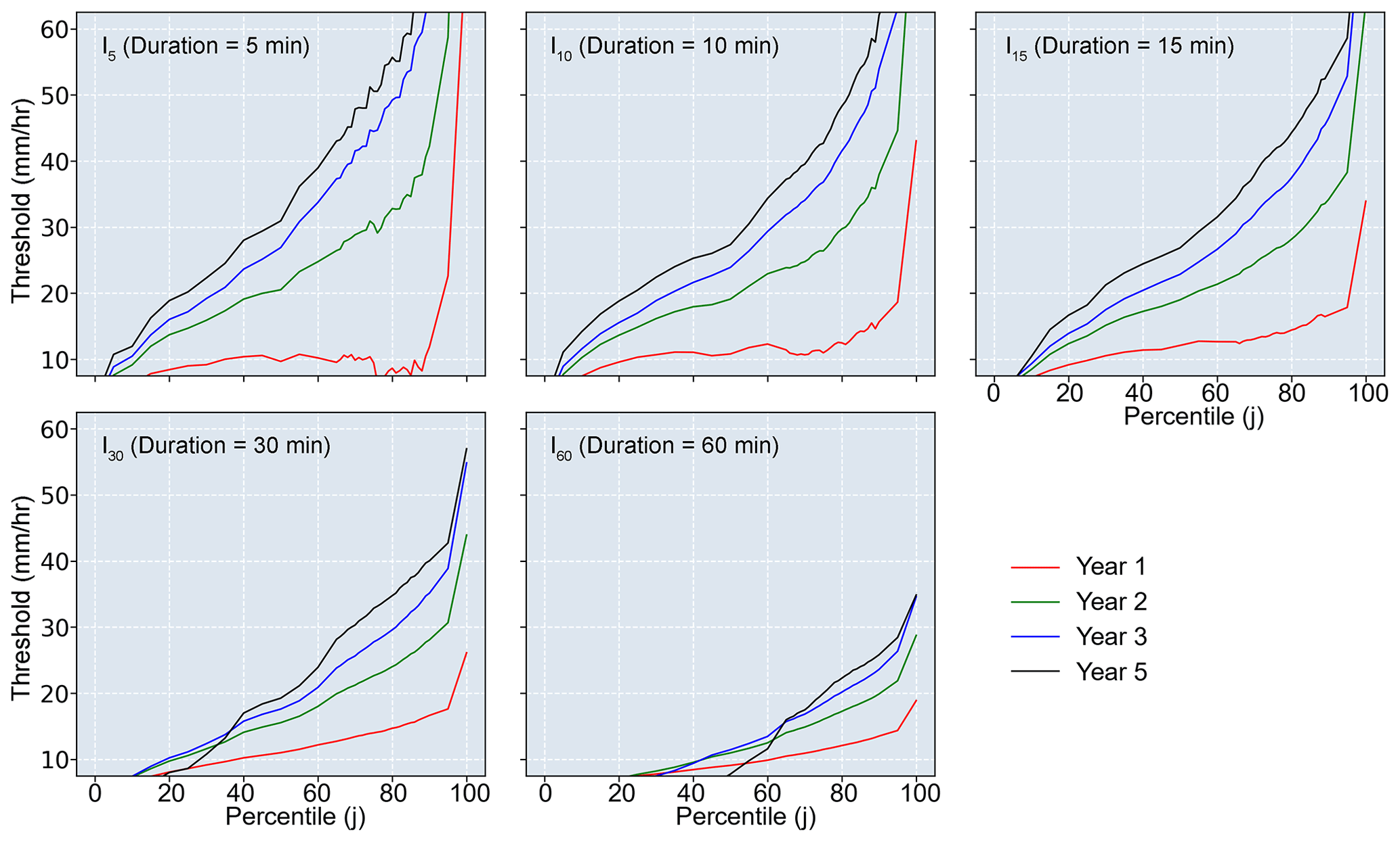
Figure 4 The rainfall intensity–duration threshold for flash floods derived from the best linear relation for different durations and percentiles of the most intense rainfall field in post-fire years 1, 2, 3, and 5.

The second approach for determining rainfall ID thresholds is based on a receiver operating characteristic (ROC) analysis following Staley et al. (2013). We assess the utility of a potential threshold (e.g. $I_{\mathrm{30}}^{\mathrm{50}}=\mathrm{20}\mathrm{mm}{\mathrm{h}}^{-\mathrm{1}}$), by computing the threat score (TS) associated with using that threshold to define the transition between rainstorms that produce flash floods and those that do not. The TS, as one of the ROC utility functions, measures the fraction of forecast events that were correctly predicted:

$$\begin{array}{}\text{(3)}& \mathrm{TS}={\displaystyle \frac{\mathrm{TP}}{\mathrm{TP}+\mathrm{FP}+\mathrm{FN}}},\end{array}$$

where TP, FP, and FN denote a true positive, false positive, and false negative, respectively. Flash flood occurrence (true or false) is determined by comparing the peak discharge of each simulated hydrograph with the flash flood level (15.3 m³ s⁻¹). A TP represents an event where rainfall rates exceed the threshold (e.g. $I_{\mathrm{30}}^{\mathrm{50}}=\mathrm{20}\mathrm{mm}{\mathrm{h}}^{-\mathrm{1}}$), and a flash flood occurred. An FP represents an event where rainfall rates exceed the threshold, but no flash flood occurred. FN events occur when rainfall rates were below the threshold, yet a flash flood occurred. The optimal TS is 1, meaning use of the threshold resulted in no false positives or false negatives.

For a given rainfall intensity metric (e.g. the peak 75th percentile of I₃₀, $I_{\mathrm{30}}^{\mathrm{75}}$, in year 1), we calculated TS for intensities ranging from 0–100 mm hr⁻¹ at 0.01 mm h⁻¹ intervals (Fig. 5). We then identified the threshold associated with the maximum TS (TS_max). The intensity associated with TS_max is the optimal threshold for that rainfall metric (Fig. 6). We determined the optimal threshold associated with each of the 495 rainfall metrics for each post-fire year (1, 2, 3, and 5) (Fig. 7). We also estimated the 95 % CI of TS and rainfall ID threshold for each year by performing bootstrapping resampling with 50 replications.

Figure 5 Threat score (TS) of the peak 75th percentile of I₃₀ in post-fire year 1. (a) Relationship between rainfall intensity and TS; (b) Scatter plots of positive (flood, red circle) and negative (no flood, hollow circle) with the rainfall intensity associated with the maximum TS.

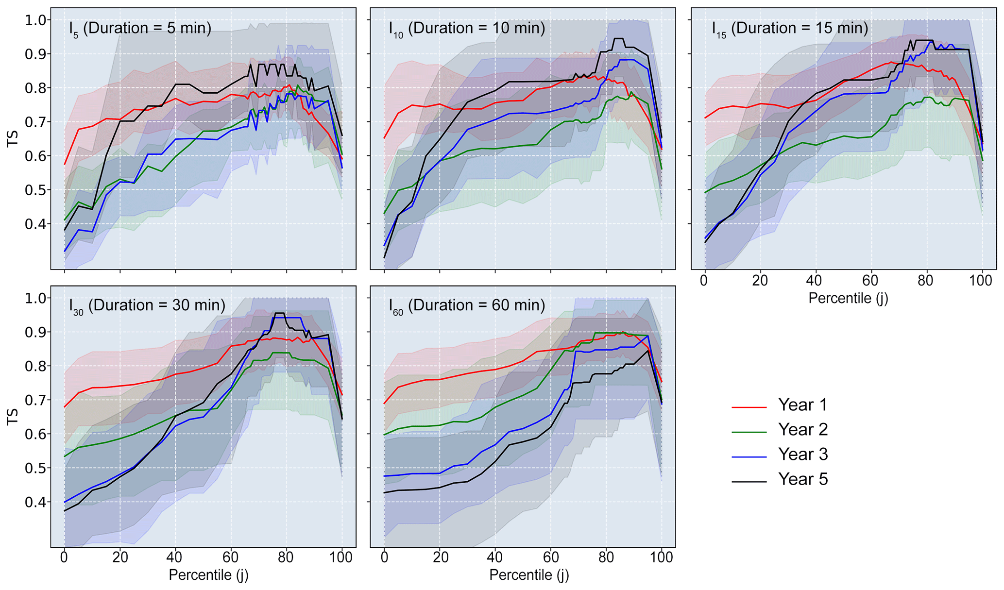
Figure 6 The threat scores (TS_max) associated with flood occurrence and $I_D^j$ in post-fire years 1, 2, 3, and 5. Data used to analyze are from events with peak discharge greater than 2 m³ s⁻¹.

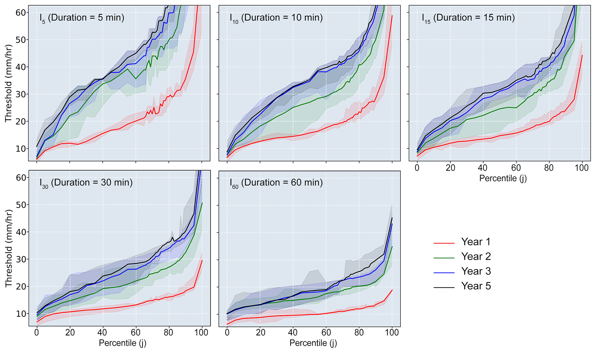
Figure 7 The rainfall intensity threshold for flash flood derived from the maximum of TS for different durations and percentiles of the most intensive rainfall field in post-fire years 1, 2, 3, and 5.

4 Results

4.1 Optimal summary metrics for defining rainfall ID thresholds

Linear regression analyses suggest that there is a stronger relationship between $I_D^j$ and peak discharge (Q) as j increases, with the exception of a rapid drop off in R² for j>95 (Fig. 3). In post-fire year 1, the maximum R² increases with duration (D) from a value of 0.72 associated with $I_{\mathrm{05}}^{\mathrm{95}}$, to 0.75 associated with $I_{\mathrm{10}}^{\mathrm{85}}$, to 0.80 associated with $I_{\mathrm{15}}^{\mathrm{72}}-I_{\mathrm{15}}^{\mathrm{87}}$, to 0.87 associated with $I_{\mathrm{30}}^{\mathrm{81}}$, to 0.89 associated with $I_{\mathrm{60}}^{\mathrm{89}}$. In post-fire years 2–5, the R² values associated with durations of 5, 10, and 15 min were maximized (0.79–0.86) within a window from the 60th–95th percentiles. The optimal rainfall threshold for flash floods (based on regressions of Q as a function of $I_D^j)$ increased from 10.1 mm h⁻¹ of $I_{\mathrm{60}}^{\mathrm{89}}$ (the 89th percentile of 60 min peak rainfall field) in year 1 to 44.6 mm h⁻¹ of $I_{\mathrm{15}}^{\mathrm{90}}$ (the 90th percentile of 15 min peak rainfall field) in year 5 (Fig. 4; Table 2). More generally, averaging rainfall intensity over a duration of 15 min and choosing a percentile, j, of approximately 75–90 produced an R² of approximately 0.80 or greater for all post-fire years (Fig. 3). None of the other rainfall summary metrics performed this well across all post-fire years.

Table 2 The linear regression-based optimal rainfall ID metrics and corresponding rainfall thresholds for flash floods in post-fire years 1–5.

Note: we denote the peak jth percentile of I_D (rainfall intensity over a duration D) as $I_D^j$. For example, $I_{\mathrm{15}}^{\mathrm{88}}$ is the peak value of the 88th percentile of I₁₅ (rainfall intensity over 15 min).

Thresholds derived using the ROC method yielded broadly similar trends. The maximum threat score, TS_max, generally increased with j up to a point (approximately j=90) and then began to decrease regardless of the choice of duration (D) (Fig. 6). The highest threat scores (TS), regardless of post-fire year or duration, were generally associated with the 70th–95th percentiles. For events in years 1–2, TS_max (0.90) occurs between $I_{\mathrm{60}}^{\mathrm{76}}$ and $I_{\mathrm{60}}^{\mathrm{86}}$ (the 76th–86th percentile of the peak I₆₀ rainfall field); for events in years 3–5, the TS_max (0.94–0.96) occurs around $I_{\mathrm{30}}^{\mathrm{75}}$ (the 75th percentile of the peak I₃₀ rainfall field). The optimal rainfall threshold for a flash flood increased from $I_{\mathrm{60}}^{\mathrm{86}}=\mathrm{12.9}\mathrm{mm}{\mathrm{h}}^{-\mathrm{1}}$ (the 86th percentile of 60 min peak rainfall field) in year 1 to $I_{\mathrm{30}}^{\mathrm{76}}=\mathrm{34.9}\mathrm{mm}{\mathrm{h}}^{-\mathrm{1}}$ (the 76th percentile of 30 min peak rainfall field) in year 5 (Table 3; Fig. 6). Averaging rainfall intensity over a duration of 30 min and choosing a percentile, j, of approximately 75–90 leads to threat scores of approximately 0.8 or greater for all post-fire years. Other metrics did not perform this well, on average, across all post-fire years.

4.2 Increases in rainfall intensity thresholds with time since fire

The rainfall intensity thresholds at each percentile increased substantially from post-fire year 1 to 5 (Figs. 4 and 7). However, the increase from year 1 to 2 is considerably larger than that from year 2 to 3 or from year 3 to 5. Taking the $I_{\mathrm{30}}^{\mathrm{75}}$ (the 75th percentile of the peak I₃₀ rainfall field) as an example due to its strong performance as a threshold for all post-fire years, the thresholds based on linear regression analyses in years 1, 2, 3, and 5 are 16.8, 23.2, 26.9, and 27.6 mm h⁻¹, respectively; the ROC-based $I_{\mathrm{30}}^{\mathrm{75}}$ thresholds in years 1, 2, 3, and 5 are 16.0, 26.9, 32.6, and 34.5 mm h⁻¹, respectively (Fig. 7).

We are also able to use the model to assess the individual impacts of temporal changes in K_sh and n_c on temporal variations in the flash flood threshold. If K_sh is allowed to vary from year to year (Table 1) and n_c is held fixed at its calibrated value for year 1, then ROC analysis indicates that the optimal threshold of $I_{\mathrm{30}}^{\mathrm{75}}$ still increases with time since fire (Fig. 8). However, it increases slower than the case where both K_sh and n_c are allowed to vary with time (Fig. 8). If n_c is allowed to vary from year to year (Table 1) and K_sh is held fixed at its calibrated value for year 1, then ROC analysis indicates that the optimal threshold associated with $I_{\mathrm{30}}^{\mathrm{75}}$ increases from year 1 to year 2 but then stays roughly constant as time increases (Fig. 8). Therefore, changes in K_sh and n_c both play important roles in determining the degree to which the flash flood threshold increases from year 1 to year 2, but further increases in the threshold in years 3 through 5 are driven mainly by increases in K_sh as a function of time since fire.

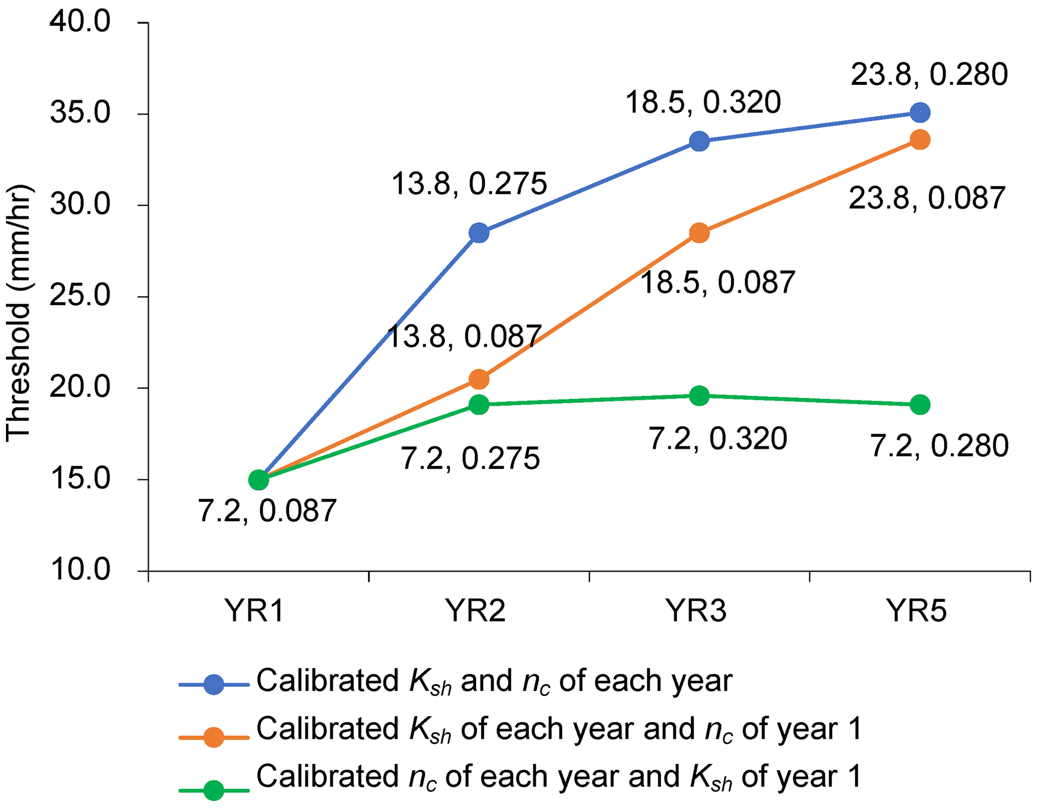
Figure 8 The ROC-based thresholds for $I_{\mathrm{30}}^{\mathrm{75}}$ in each year with different model settings. Pairs of K_sh (saturated hydraulic conductivity on hillslopes) and n_c (Manning's n in channels) in each model are given along with the data points.

5 Discussion

5.1 Optimal metrics of rainfall intensity and duration for flood warning

Rain gage records, which provide rainfall intensity data at a single point, are often used to define rainfall ID thresholds in debris-flow and flash-flood studies (e.g. Moody and Martin, 2001; Cannon et al., 2008, 2011; Guzzetti et al., 2008; Kean et al., 2011; Staley et al., 2013; Raymond et al., 2020; McGuire and Youberg, 2020). Using point source data to define thresholds for debris flows and flash floods is ideal when rainfall intensity does not vary substantially over the watershed, an assumption that is most appropriate for watershed areas less than several square kilometers. Radar-derived rainfall data has the advantage of providing spatially explicit information over an entire watershed at a high-temporal resolution (e.g. 5 min). However, one challenge in using radar-derived precipitation to define thresholds is the need to condense spatially and temporally variable rainfall intensity information down to a single rainfall intensity metric. Regardless of whether the approach to determining an ID threshold involves fitting empirical relationships (e.g., Moody and Martin, 2001; Cannon et al., 2008) or using ROC analysis (e.g., Staley et al., 2013), a single metric is required to represent the rainfall intensity for each duration.

We summarized spatially variable rainfall intensity data over the watershed by computing the peak value of $I_D^j\left(t\right)$, the jth percentile of I_D(t) for each rainstorm. We used two different techniques, one based on a linear regression analysis and one based on ROC analysis (Fig. 2), to define thresholds for flash floods in post-fire years 1, 2, 3, and 5. Although the optimal metrics produced by the two approaches are not identical, they are generally similar in each post-fire year. In particular, high R² and TS_max values are associated with metrics of the peak 75th–85th percentile of rainfall intensity averaged over 15–60 min ($I_D^j$ for $\mathrm{75}\le j\le \mathrm{85},\mathrm{D}=\mathrm{15},\mathrm{30},\mathrm{60})$. In other words, a good indicator of the potential for a flash flood is the presence of intense pulses of rainfall over durations of 15–60 min that cover at least 15 %–25 % of the watershed (Fig. 9). This finding highlights the ability of rainstorms to produce flash floods even if they do not cover the majority of the watershed with intense rainfall. If rainfall over the majority of the watershed was required to produce flash floods, then we would expect that $I_D^j$ with j<50 would be a better predictor of flash floods.

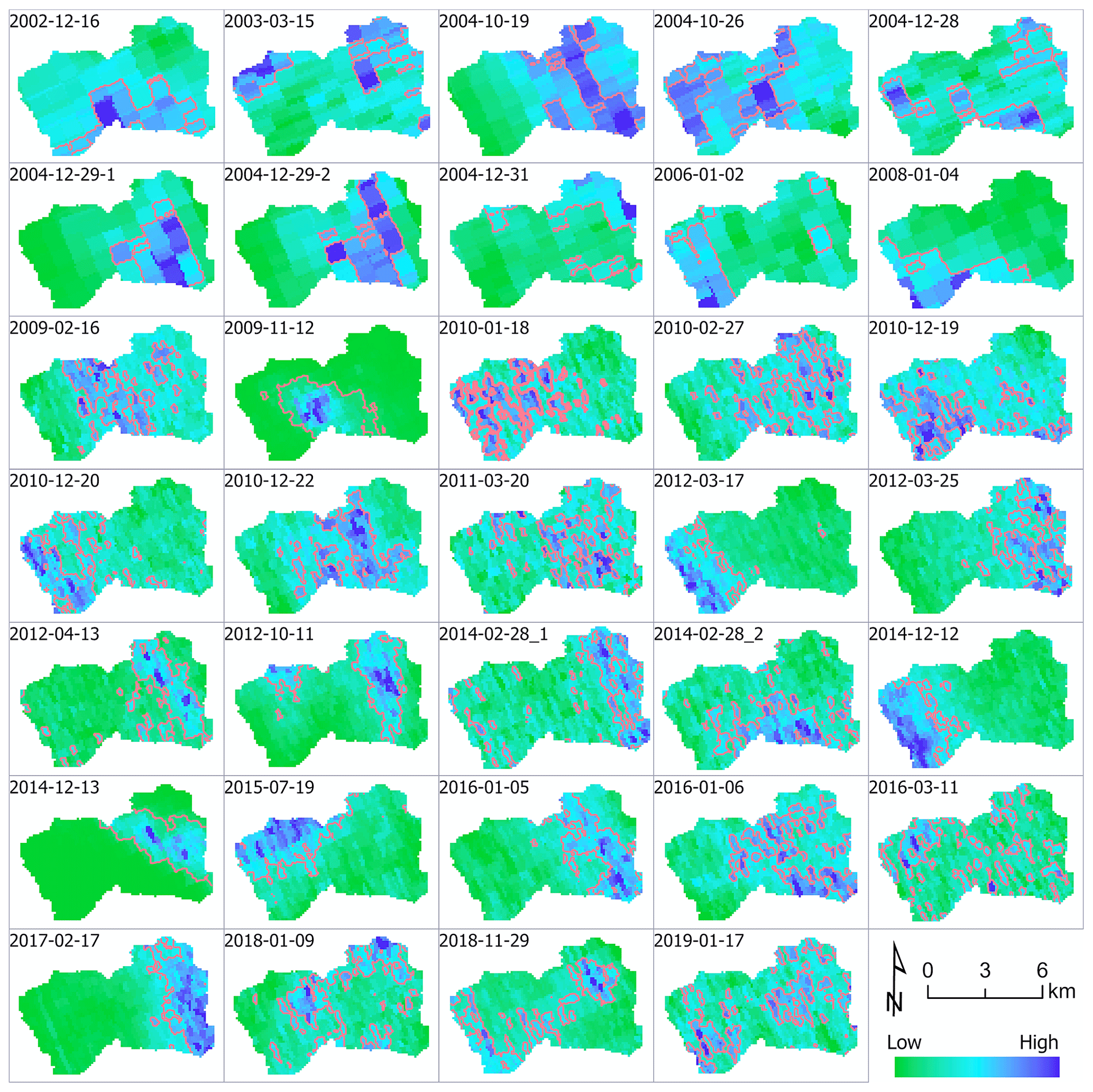
Figure 9 Snapshots of the spatial patterns of $I_{\mathrm{30}}^{\mathrm{75}}$ of 34 unique storms. The peak jth percentile of I_D (rainfall intensity over a duration D) is denoted as $I_D^j$. $I_{\mathrm{30}}^{\mathrm{75}}$ is the peak value of the 75th percentile of I₃₀ (rainfall intensity over 30 min). Red contours delineate the pixels with rainfall intensities larger than $I_{\mathrm{30}}^{\mathrm{75}}$ of each storm.

Previous work has also identified that 30 min rainfall intensity works well for predicting flash floods and debris flows (Moody and Martin, 2001; Kean et al., 2011; Staley et al., 2013). The finding that $I_{\mathrm{15}}^j$, $I_{\mathrm{30}}^j$, and $I_{\mathrm{60}}^j$ work best as thresholds when $\mathrm{75}\le j\le \mathrm{85}$ could be helpful when issuing flash flood warnings based on radar-derived precipitation estimates or data from several real-time rain gages within a watershed. Current operational forecast models such as the High-Resolution Rapid Refresh model have a horizontal resolution of 3 km and minimum temporal resolution of 15 min (Benjamin et al., 2016; NOAA, 2021a), such that it is feasible to use either $I_{\mathrm{15}}^j$, $I_{\mathrm{30}}^j$, or $I_{\mathrm{60}}^j$ in an operational forecast setting. Where sufficient operational NEXRAD weather radar coverage is present, radar-derived precipitation estimates such as the Multi-Radar/Multi-Sensor System (MRMS; Zhang et al., 2016) can provide near-real-time precipitation estimates at 1 km and as fine as 15 min temporal resolution (NOAA, 2021b). In the case of poor radar coverage, gap-filling radars may be temporarily deployed or installed (e.g., Jorgensen et al., 2011; Cifelli et al., 2018) to provide information necessary for accurate precipitation estimates. While the magnitude of rainfall thresholds estimated here may only work for similar, recently burned watersheds within the San Gabriel Mountains, this work provides a general methodology for exploring reliable predictors of post-fire flash floods for other watersheds and settings. Further testing is needed in watersheds with different watershed sizes, topographic characteristics, landscapes, and burn severity patterns.

Table 3 The ROC-based optimal metrics of rainfall ID and corresponding rainfall thresholds for flash floods in post-fire year 1–5.

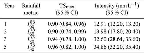
Note: we denote the peak jth percentile of I_D (rainfall intensity over a duration D) as $I_D^j$. For example, $I_{\mathrm{60}}^{\mathrm{86}}$ is the peak value of the 86th percentile of I₆₀ (rainfall intensity over 60 min).

Several limitations are present in this work. First, we assess a small number of storm events (34) in the area as we are limited by the length of radar and gage records as well as the number of events that impact the indicator rain gages, though applying the five Z-R relationships provides us with 170 rainfall realizations to assess. We prefer the use of observed rainfall data (radar and gauges) over simulated products, such as output from a rainfall generator (e.g., Zhao et al., 2019; Evin et al., 2018), as the radar is able to capture the spatial and temporal patterns of rainfall intensity in the study area's complex terrain. Though rainfall generators have advanced to represent some synoptic-to-mesoscale features, such as frontal and convective precipitation (e.g., Zhao et al., 2019), they are fundamentally designed to represent statistical characteristics of rainfall in places with limited observations (Wilks and Wilby, 1999) and cannot be relied upon to replicate small-scale storm characteristics in complex terrain (e.g., Camera et al., 2017). Future work could compare results from this hydrological modeling experiment with observed versus simulated rainfall. Second, the challenges of using Z-R relationships to convert reflectivity into precipitation also present challenges in accurately representing precipitation values. This can be addressed in future work through studies to constrain Z-R relationships for storms producing intense rainfall in this region and through the deployment or installation of high-resolution gap-filling radars (e.g., Johnson et al., 2020).

Figure 10 Box plots showing the runoff coefficient and peak discharge of flash floods in post-fire years 1, 2, 3, and 5. The numbers of flash floods in each year are displayed next to the box.

5.2 The role of hydrological models in rainfall intensity threshold estimation

In this study we employed the K2 model calibrated by Liu et al. (2021) to parameterize hydrologic changes affecting Hortonian overland flow within a 5-year period following fires. Hillslope saturated hydraulic conductivity (K_sh=7.2 mm h⁻¹) and hydraulic roughness in channels (n_c=0.087 s m${}^{-\mathrm{1}/\mathrm{3}})$ were lowest immediately after fire (Table 1), resulting in high runoff coefficients and low rainfall thresholds in post-fire year 1. In later years, with K_sh and n_c gradually increasing (Table 1), more rainfall infiltrated into the soil and there was increased attenuation of flood peaks. Simulations indicate that the number of flash-flood-producing rainstorms decreased from 59 in year 1 to 25, 18, and 16 in years 2, 3, and 5, respectively. Runoff coefficients and peak discharge of simulated hydrographs also decreased with time since fire (Fig. 10). Given the same precipitation ensemble, the likelihood of flash floods significantly decreased with time. The peak discharge produced by the highest intensity rainfall event with $I_{\mathrm{60}}^{\mathrm{75}}$ of 51.8 mm h⁻¹ was 554.0 m³ s⁻¹ in the first year after the fire, which is 3 times greater than the peak discharges of 157.5 m³ s⁻¹ in year 3 and 161.2 m³ s⁻¹ in year 5 produced by the same rainstorm. From a flood hazard perspective, the downstream area may be exposed to a 1000-year flood under recently burned conditions (less than 1 year since the fire), whereas the discharge produced in years 3 and 5 amounts to roughly a 30- to 40-year flood (Fig. S3).

We were also able to perform numerical experiments to quantify the relative importance of temporal changes in K_sh and n_c on temporal variations in the flash flood threshold (Fig. 8). Results suggest that changes in vegetation and grain roughness, which are likely to influence n_c, throughout the recovery process are less important for determining flash flood potential in our study area relative to changes to saturated hydraulic conductivity on hillslopes. It is worth noting that temporal changes in other model parameters (e.g., hydraulic roughness on hillslopes, capillary drive) may play more of a role in driving changes in post-fire flash flood thresholds in other settings. In this study, however, we focus on changes in K_sh and n_c because Liu et al. (2021) were able to detect temporal changes in n_c and K_sh through time and were unable to detect similar temporal changes in other hydrologic parameters (e.g., hydraulic roughness on hillslopes, capillary drive) due to their relatively minor influence on runoff in the study watershed.

In this study, the optimal flash flood thresholds increased from $I_{\mathrm{30}}^{\mathrm{75}}=$ 16.0–16.8 mm h⁻¹ in post-fire year 1, to 23.2–26.9 mm h⁻¹ in year 2, and 27.6–34.5 mm h⁻¹ in post-fire year 5 (Figs. 4 and 7; Tables 2–3). In the San Gabriel Mountains and nearby San Bernardino and San Jacinto mountains, Cannon et al. (2008) estimated rainfall thresholds of I₃₀=9.5 mm h⁻¹ for flash floods and debris flows in the first winter rainy season following fires. They found that the thresholds for flash floods and debris flows increased to I₃₀=19.8 mm h⁻¹ in post-fire year 2. The thresholds that we infer from hydrological modeling are greater than those reported by Cannon et al. (2008), which may be partly due to differences in (1) the data and methods used and (2) the size of the studied watersheds. Our results are driven by a hydrological model, forced with a radar precipitation ensemble that consists of 170 rainstorms that contain a variety of storm types that impact southern California. The occurrence of a flash flood is based on exceedance of the maximum channel capacity and we summarize temporal changes in the rainfall ID threshold using $I_{\mathrm{30}}^{\mathrm{75}}$ since we find this to be a reliable metric for all post-fire years included in this study. In contrast, Cannon et al. (2008) established rainfall ID relations by using observations of rainstorms and hydrological responses in the 2 years following fires in 87 small watersheds (0.2–4.6 km²). They base their thresholds on rainfall characteristics that produced either flash floods or debris flows, whereas we focus solely on flash floods. In their dataset, flash floods and debris flows were identified by investigating flood and debris flow deposits at the outlet of those small watersheds in the field. Despite differences in the magnitude of the thresholds, the increase in the threshold from post-fire year 1 to year 2 in both studies are quite close. This agreement provides support for the use of simulation-based approaches to inform temporal shifts in rainfall ID thresholds.

During the recovery process, increasing thresholds for flash floods and debris flows have also been identified in other areas at different scales by either observation- or simulation-based studies, such as hillslopes in the Colorado Front Range (Ebel, 2020) and small watersheds in Australia (Noske et al., 2016). The consistent increase in rainfall ID thresholds with time since fire in different geographic and ecological zones implies that hydraulic and hydrological models may be useful tools for exploring how the transient effects of fires translate into changes in water-related hazards. The role of hydraulic and hydrological models becomes particularly more important when historic data are limited and traditional empirical methods are impractical for defining thresholds.

6 Conclusions

We used 250 m, 5 min radar-derived precipitation estimates over a 41.5 km² watershed in combination with a calibrated hydrological model to estimate rainfall intensity–duration thresholds for post-fire flash floods as a function of time since fire. The main outcomes of this study are (1) identification of optimal radar-derived rainfall metrics for post-fire flash flood prediction in southern California, (2) estimates of temporal changes in rainfall ID thresholds for flash floods following disturbance in a chaparral-dominated ecosystem, and (3) a methodology for using a hydrological model to assess changes in post-fire flash flood thresholds.

Results indicate that thresholds based on the 75th–85th percentile of peak rainfall intensity averaged over 15–60 min perform best at predicting the occurrence of a flash flood in our study area. In other words, a flash flood tends to be produced when rainfall intensity over 15 %–25 % of the watershed area exceeds a critical value. A threshold based on $I_{\mathrm{30}}^{\mathrm{75}}$ performs consistently well for post-fire years 1, 2, 3, and 5, although the magnitude of the threshold increases with time since fire. For the watershed studied, the $I_{\mathrm{30}}^{\mathrm{75}}$ threshold increases from 16.0–16.8 mm h⁻¹ for year 1 to 23.2–26.9, 26.9–32.6, and 27.6–34.5 mm h⁻¹, for years 2, 3, and 5 respectively. Increases in the threshold value of $I_{\mathrm{30}}^{\mathrm{75}}$ can be primarily attributed to increases in K_sh rather than n_c during the hydrological recovery process. The increase in the magnitude of the threshold from year 1 to year 2 is consistent with previous observations from nearby areas in southern California. Results provide a methodology for using radar-derived precipitation estimates and hydrological modeling to estimate flash flood thresholds for improved warning and mitigation of post-fire hydrologic hazards. Thresholds developed through these methods can then be built into operational tools that use incoming radar data to evaluate the flash flood hazard in near-real-time or precipitation forecasts to evaluate potential for flash flood hazard in burned watersheds.