Machine learning models to predict myocardial infarctions from past climatic and environmental conditions

Myocardial infarctions (MIs) are a major cause of death worldwide, and both high and low temperatures (i.e. heat and cold) may increase the risk of MI. The relationship between health impacts and climate is complex and influenced by a multitude of climatic, environmental, socio-demographic and behavioural factors. Here, we present a machine learning (ML) approach for predicting MI events based on multiple environmental and demographic variables. We derived data on MI events from the KORA MI registry dataset for Augsburg, Germany, between 1998 and 2015. Multivariable predictors include weather and climate, air pollution (PM₁₀, NO, NO₂, SO₂ and O₃), surrounding vegetation and demographic data. We tested the following ML regression algorithms: decision tree, random forest, multi-layer perceptron, gradient boosting and ridge regression. The models are able to predict the total annual number of MIs reasonably well (adjusted R²=0.62–0.71). Inter-annual variations and long-term trends are captured. Across models the most important predictors are air pollution and daily temperatures. Variables not related to environmental conditions, such as demographics need to be considered as well. This ML approach provides a promising basis to model future MI under changing environmental conditions, as projected by scenarios for climate and other environmental changes.

1 Introduction

Myocardial infarctions (MIs) are a major cause of cardiovascular-related mortality and morbidity. The estimated prevalence of MI worldwide in 2015 was close to 16 million, with 33 000 years lived with disability attributed to the condition (Vos et al., 2016). In light of ageing western societies as well as ongoing environmental and climatic changes, which have been identified as important risk factors, MI is likely to remain a considerable burden to health systems in the future (e.g. Khraishah et al., 2022). It is therefore paramount to deepen the understanding of the complex interplay between environmental and other risk factors and their effect on MI and to estimate their expected future development.

Epidemiological research has shown that both high and low air temperature extremes (i.e. extreme cold and heat) can play an important role in triggering acute MI (Chen et al., 2019; Wolf et al., 2009; Sun et al., 2018). This is especially apparent in winter, when most of the MI events are observed. Most previous studies (e.g. with registry data) have reported significant cold effects on MI occurrence (e.g. The Eurowinter Group, 1997; Schwartz et al., 2004; Wolf et al., 2009; Bhaskaran et al., 2010), whereas fewer studies have observed increased risk of MI triggered by heat exposures so far (e.g. Bhaskaran et al., 2012; Madrigano et al., 2013; Chen et al., 2019). Severe periods of heat as encountered during heat waves are likely to occur with higher frequency, intensity and duration due to anthropogenic climate change, even if limited to warming levels between 1.5 and 2 ^∘C (Sieck et al., 2021). Increasing levels of urbanisation entail higher levels of exposure to heat as well, due to the urban heat island effect (e.g. Feng et al., 2014; Zhang et al., 2009). Air pollution is another environmental factor known to potentially trigger MI after periods of intense short-term exposure (e.g.  Peters et al., 2004; Mustafić et al., 2012) but also to increase the risk in association with elevated long-term exposure (Cesaroni et al., 2014; Wolf et al., 2021; Rajagopalan et al., 2018). Moreover, the elderly are particularly vulnerable to MI, exacerbating the potential adverse effects in light of the demographic ageing expected in developed countries, such as in Germany (Schmidt et al., 2013; Rai et al., 2019).

A key issue in understanding current and future health impacts is the inclusion of a multitude of processes and circumstances that influence the health outcomes (Roth, 2020) in quantitative models. For MI, these include the occurrence of high- and low-temperature events, air quality, the presence of water bodies, and vegetation and characteristics of the built environment. Although the relevance of humidity for MI has not been confirmed (e.g. Schwartz et al., 2004), it is often included when studying human health impacts (Davis et al., 2016). For instance, high temperatures are often perceived as more stressful under very humid conditions. Hot and strongly saturated air carries less oxygen and interferes with transpiration as the main mechanism of cooling the human body (Havenith, 2005). Therefore, the same temperature can be perceived as more straining if humidity is high as well. Changes in the exposed population, such as their age, their health status and underlying diseases, are important as well. Therefore, not only can future health risks from climate change be estimated from changes in (extreme) weather, but it is also critically important to account for all these other relevant factors (Vanos et al., 2020). Finally, health interventions such as heat health action plans and improved healthcare have been shown to reduce health risks from extreme temperatures (see for instance Achebak et al., 2019). But also policies related to climate change, such as reduced traffic emissions, are expected to lead to a reduction in disease burden (Laverty et al., 2021).

For more reliable estimations of potential future risks, multiple variables must be incorporated into prediction models. In addition, several of the relations between environmental and other factors and health outcome are only partially known. This is where data-driven approaches are particularly useful, as they can provide accurate estimations of complex processes, taking up many variables and also accounting for complex and non-linear relations. Machine learning (ML) approaches are now being tested widely for environmental studies (Reichstein et al., 2019), and they are also increasingly used to estimate social and economic impacts of environmental extremes such as floods and windstorms (Merz et al., 2013; Wagenaar et al., 2017, 2021). ML, however, has only recently been applied to health impact modelling. Several studies have employed statistical methods as well as ML to predict infectious diseases, such as malaria transmissions (Zinszer et al., 2012; Sewe et al., 2017). Zhang et al. (2014) studied heat-related mortality and identified relevant temperature and humidity variables using random forests. Other studies applied ML to evaluate the risk for MI or to predict acute MI based on data such as patient history, blood markers or electrocardiogram, but they lack an environmental dimension (e.g. Tamarappoo et al., 2021; Commandeur et al., 2020).

In this study we employ several ML algorithms in a data-driven setting, using a range of meteorological, environmental, demographic and health variables on preceding days. We estimate the importance of the predictive variables in the models. We also assess the effects on different subgroups, depending on location (urban/rural), as these may exhibit different vulnerabilities (Gabriel and Endlicher, 2011), and patient characteristics (age, smoking and diabetes). The ML models that are presented can be used to estimate future health outcomes, using a set of scenarios for changes in climatic, environmental and demographic variables. Instead of using an approach based on time series modelling (see e.g. Armstrong, 2006; Chen et al., 2018), we employ multivariate ML regression models. These models do not require the presupposition of a known exposure–response relationship. Also, our study is aimed towards developing models to make long-term projections at climate timescales (30 years). At such timescales underlying statistical properties may change gradually, which would not be reflected by any prescribed exposure–response function based on historic or current data. Contrary to other studies, we also do not account for seasonal effects. Instead, we solely rely on a data-driven approach in which we make no a priori assumptions about the relationship between features and the health outcome. While this does not allow for an explicit decomposition of the time series into, for example, trend, seasonality and random effects, it might generalise better when applied to an ensemble of climate simulations in which the statistics of the features may have changed drastically compared to the historical training data.

We expect that none of the risk factors that are included in our models is strong enough to directly trigger MI in an otherwise healthy person. Instead, these environmental and demographic factors must be assumed to increase the statistical likelihood of vulnerability to MI over longer periods of time. Many of the risk factors that we cover in this study can modify this individual likelihood of suffering from MI. In light of this, we do not expect the models to be able to accurately provide predictions on a daily basis. However, our research motivation is to eventually estimate the long-term tendencies in MI due to climate change. We therefore decided to aggregate our model results on an annual basis. This should allow for some of the inherent randomness to average out and allow a more statistical view of MI occurrence over annual and interannual timescales.

In Sect. 2, we present the methods used to develop the ML models. In Sect. 3, we describe the input data for our data-driven approach. In Sect. 4 the results of the simulations and their performance are given. In Sect. 5 we discuss the results and give an outlook for using the models to project future MI events, and finally in Sect. 6 we provide the conclusions.

2 Methods

In this section, we present the approach to modelling the occurrence of MI events from a large variety of data and discuss the ML methods that were applied. We also consider correlations among the features and describe how we selected suitable parameters for the ML algorithms.

2.1 A supervised learning problem for MI events

ML models can comprise classification- or regression-based algorithms. In this study, we focus solely on regression methods. The registry data are case-only; i.e. by design each participant is bound to have a MI.

The target variable in our case is the time series of daily events of MI observed in the study region. In addition, the co-occurring environmental variables that have a plausible causal relation to this target variable are collected and used as predictors in the training process. We use the scikit-learn package for performing the calculations (see Pedregosa et al., 2011; Pedregosa et al., 2022). The figures use colours chosen with disability friendliness in mind (Crameri et al., 2020).

For any given day d let y_d be the number of MI events and x_i,d the value of the ith predictive variable on that day (e.g. daily maximum temperature or daily mean PM₁₀). To work with standard regression algorithms, a fixed number of features must be selected and together with the target value y_d be provided as training input. The variables x_i,d represent a time series, and therefore only a subset of them should be selected as a feature of the regression problem, namely the conditions on the day of prediction. Past conditions, however, might also have an influence on current events, both long- and short-term. The sliding window method allows for this by selecting the features with a lag n, referred to as the window size. The merits of allowing for shorter or longer memories are difficult to estimate. For instance, the effects of extremely high temperatures on MI are generally expected to be short-term (Breitner et al., 2014), ranging from immediate effects to up to 3 weeks lag. The vector of features, i.e. the training (or test) instance on day d, is then given as

$$\begin{array}{}\text{(1)}& \begin{array}{rl}{\mathit{x}}_{\mathrm{d}}=& \left(x_{\mathrm{1},\mathrm{d}-n+\mathrm{1}},x_{\mathrm{1},\mathrm{d}-n+\mathrm{2}},\mathrm{\dots },x_{\mathrm{1},\mathrm{d}},x_{\mathrm{2},\mathrm{d}-n+\mathrm{1}},\mathrm{\dots },x_{\mathrm{2},\mathrm{d}},\right.\\ & \left.x_{m,\mathrm{d}-n+\mathrm{1}},\mathrm{\dots },x_{m,\mathrm{d}}\right),\end{array}\end{array}$$

where n is the windows size and m the number of variables. Each predictive variable then yields n features, and the total number of features for this problem is n⋅m. Accumulating the x_d and y_d for all days into a matrix X and a vector y yields input that can directly be used with the scikit-learn regression algorithms. We applied the five ML methods and associated scikit-learn classes, listed in Table 1 with their abbreviations as used in the remainder of this paper. Note that some features such as the slowly changing demographic variables, were not subject to the sliding window and instead simply used the value on the day of prediction. For this study, after testing different lags between 1 and 21 d, we exclusively used a lag of n=3 d as this resulted in the best overall scores. However, in order to account for possibly longer-lasting (see Sun et al., 2018) cold effects, we added a predictor using the 21 d rolling mean of the minimum temperature.

Table 1 Regression methods used and associated scikit-learn classes.

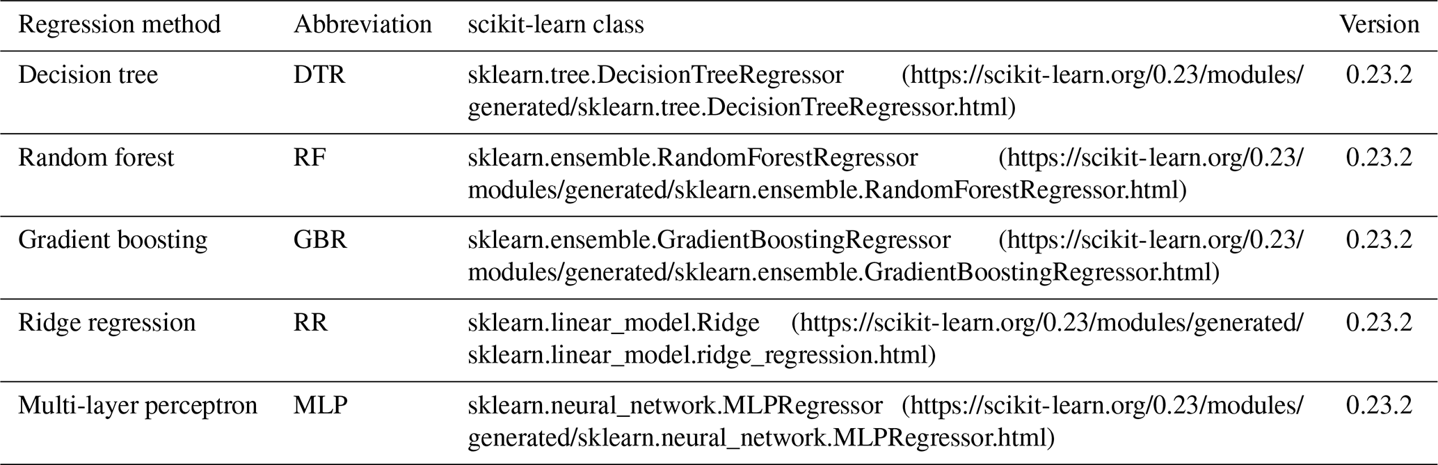
All links were accessed on 4 September 2022.

Note that throughout this paper, we use the terms predictor and feature in an interchangeable manner, namely to refer to the features of the supervised learning problem derived above: the vector X and its components.

We also added a random feature to be able to use its importance as a benchmark. Predictors less important than the random feature can be assumed to be irrelevant. Finally, we added three time variables, namely the day of the week, the day of the year and the current month.

2.2 Scaling and random split

Different magnitudes of the features can have adverse effects as the results could be biased towards those variables given in nominally large units relative to others. To avoid this, we apply the sklearn.preprocessing.StandardScaler class to the input, resulting in features that are centred around 0 with unit variance. Second, we withhold parts of the data from the training to have independent data instances for validation. We apply sklearn.model_selection.train_test_split with shuffle, resulting in a random 75 %/25 % split of the data in training and test portions. The 25 % of data not used for training the algorithms are used for validation. Splitting the data randomly means that the underlying time series lose their natural temporal order. This has implications when visualising and interpreting model results that we will cover in a later section, but it reduces the likelihood of autocorrelations (e.g. seasonal signals) present in the time series that could result in overoptimistic predictions. In order to split the data randomly, the random number generator has to be initialised with a seed. We found that different random seeds can result in significantly different results. To avoid reporting results that are strongly dependent on the chosen seed, we repeated all calculations with 100 randomly selected seeds. The result with the R² score closest to the average score of the ensemble was then selected as a representative example of model capability. Moreover, as the dependency on the random seed is likely related to unbalanced splits, we employed a simple stratification strategy. The data are stratified along the number of MI occurrences observed; i.e. data points with the same number of MIs are split among test and training in a representative way. This is especially important for rare events, such as five or more MIs in 1 d. The dependency on the random seed was substantially reduced in this way, but significant differences between different seeds could still be observed.

2.3 Feature importance

It is useful to evaluate the relative importance of different features, i.e. to measure the contribution a given feature makes to the overall prediction. In this study, we use the built-in variable importance capabilities provided by the scikit-learn package, yielding a number between 0 and 1 for each feature. The sum of all individual contributions is always equal to 1. For RR we simply relate the magnitude of the trained weights (coefficients) of the model to their associated predictors. Here, care must be taken to consider the relative magnitudes of the predictors, but this has been addressed in our study by scaling the input data. For DT, RF and GBR the importance is based on the normalised total impurity decrease, i.e. a measure of the quality of splits associated with a given feature, aggregated across the whole tree or the ensemble of trees, respectively. For MLP no variable importance is provided by scikit-learn, and we therefore constrained this part of the analysis to the four aforementioned algorithms.

2.4 Feature reduction

Correlated features can lead to an overemphasis of their influence on the target variable. This can be counteracted by choosing only one of the correlated features, usually the one that has the strongest correlation with the target variable. In our case, we aimed to include as many variables as possible that could reasonably have an effect on MI. The downside is that some features, for instance maximum, minimum and mean temperature, are highly correlated on a daily basis. A visualisation of the correlation between the predictors used in this study is shown in Fig. A8. To address this issue, we tested the option of transforming the data to a smaller feature space using principal component analysis (PCA). The resulting principal components are uncorrelated to each other, and the risk of introducing spurious or overly strong relationships into the training data is reduced while retaining most of the original information. We used sklearn.decomposition.PCA and opted to retain at least 98 % of the variance. Having the principal components as optional features allowed us to compare predictions with PCA to estimate the potential adverse effects of correlations present in our data. The results using the PCA data (not shown here) did not improve, suggesting that using the original set of features does not introduce spurious relations. Moreover, using PCA leads to a reduction in interpretability, as the principal components are linear combinations of the original features, without a clear relation to the original variables.

2.5 Hyperparameter optimisation

The ability of the ML algorithms listed in Table 1 to produce accurate predictions is dependent on the selection of appropriate hyperparameters. These parameters generally control specific aspects of the underlying methods, such as the maximum depth of a decision tree, the number of neurons in a layer or the strength of regularisation. With regularisation, a penalty is added as model complexity increases, which helps to avoid overfitting. In this study, we used the sklearn.model_selection.GridSearchCV class to optimise hyperparameters over predefined parameter spaces with 5-fold cross-validation. We used the adjusted R² as the governing score to make decisions on optimal parameters. The parameter set with the best overall score is selected. Using cross-validation allows the production of more robust generalisation error estimates without having to reserve a dedicated cross-validation set that would not be available for training. Moreover, by using folds based only on 75 % of the training data, no information from the remaining 25 % of the data is used for optimising the models and validation through parameter selection.

Due to substantial computational expense, we only optimised over rather sparse parameter spaces and a limited number of the available parameters. Table 2 shows a list of the selected hyperparameters for all the methods used as well as their optimised values. To speed up the calculations we used the Intel^® extension package for scikit-learn, called scikit-learn-intelex.

Table 2 Optimised hyperparameters marked with bold.

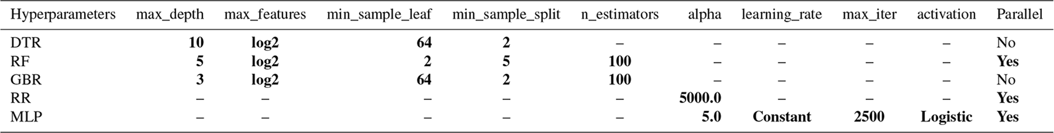
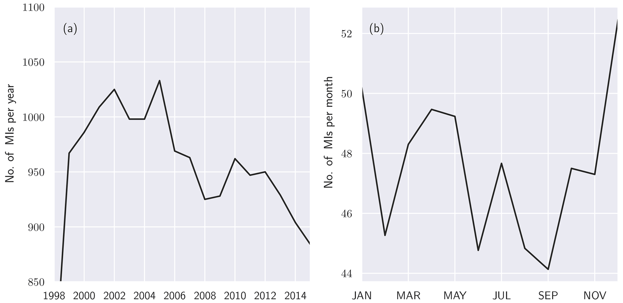
Figure 1 Number of annual MIs (a) and mean annual cycle (b) in people aged under 75 from 1985 to 2015 for the study region (city of Augsburg and counties Aichach-Friedberg and Augsburg).

3 Data

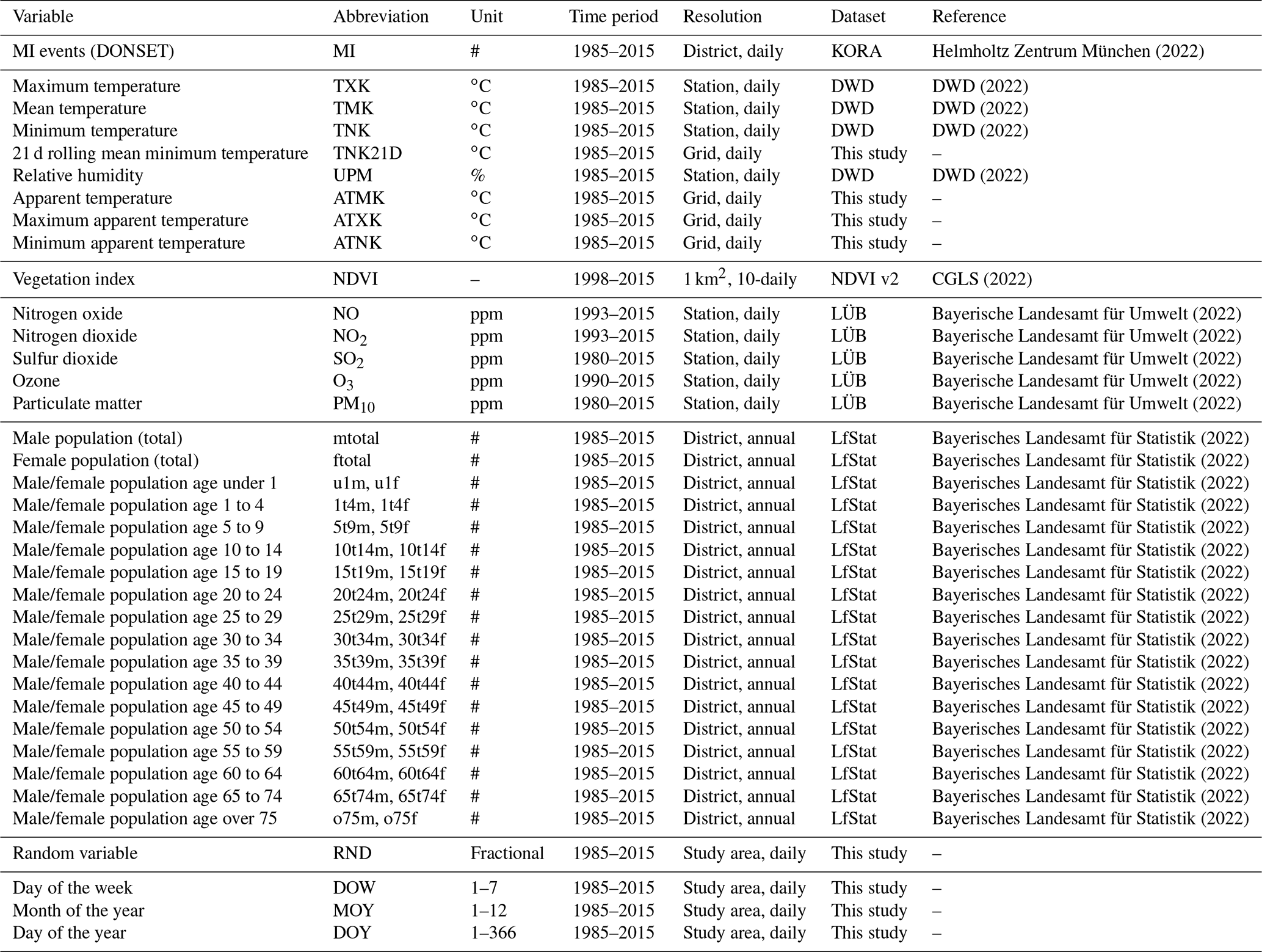
The dataset used in this study is highly heterogeneous along many dimensions, with differences ranging from file format, metadata conventions, spatial coverage (e.g. regional, local) and resolution to temporal frequency (e.g. daily, monthly, annual) and representation (e.g. raster, polygon and point data). In this section, we give an overview of the data used in this study and describe the workflow applied to homogenise and prepare these. Table 3 lists all environmental and demographic predictive variables that were used for this study in addition to the MI data, as well as the source datasets and associated references.

Helmholtz Zentrum München (2022)DWD (2022)DWD (2022)DWD (2022)DWD (2022)CGLS (2022)Bayerische Landesamt für Umwelt (2022)Bayerische Landesamt für Umwelt (2022)Bayerische Landesamt für Umwelt (2022)Bayerische Landesamt für Umwelt (2022)Bayerische Landesamt für Umwelt (2022)Bayerisches Landesamt für Statistik (2022)Bayerisches Landesamt für Statistik (2022)Bayerisches Landesamt für Statistik (2022)Bayerisches Landesamt für Statistik (2022)Bayerisches Landesamt für Statistik (2022)Bayerisches Landesamt für Statistik (2022)Bayerisches Landesamt für Statistik (2022)Bayerisches Landesamt für Statistik (2022)Bayerisches Landesamt für Statistik (2022)Bayerisches Landesamt für Statistik (2022)Bayerisches Landesamt für Statistik (2022)Bayerisches Landesamt für Statistik (2022)Bayerisches Landesamt für Statistik (2022)Bayerisches Landesamt für Statistik (2022)Bayerisches Landesamt für Statistik (2022)Bayerisches Landesamt für Statistik (2022)Bayerisches Landesamt für Statistik (2022)Bayerisches Landesamt für Statistik (2022)

Table 3 Overview of predictive variables, source datasets and their origin.

3.1 KORA MI registry

The health dataset for our study is the KORA/MONICA MI registry (see Tunstall-Pedoe et al., 1994; Holle et al., 2005), comprising records of MI events that occurred within the study region from 1985 to 2015. These data were collected at the hospitals in the Augsburg region. Each record contains the date of the MI occurrence and age and sex of the patient. Depending on availability, complementary information is given, such as the patients' residential county (Landkreis), their body mass index (BMI), smoking status and pre-existing conditions such as diabetes. Although no detailed information is provided on the location of the patient during a MI event, they can be assigned to either the urban (city of Augsburg) or one of the two rural counties (Landkreise) of the study region (Landkreis Augsburg and Aichach-Friedberg). As pointed out earlier, the individual patient-specific data could not be used as predictive data due to the nature of the regression approach, which aims to predict the gross number of MI in the population. It is, however, possible to use these data to confine investigations to subgroups, e.g. to inhabitants of either urban or rural areas, and also to the elderly or to smokers, albeit at the cost of being limited to a smaller subset of the overall data. In total the number of recorded MIs is n=34 618. Until 2008 the study was limited to participants of up to 74 years of age, with n=30 081 records total in that category. Figure 1 shows the aggregated number of MIs per year and the mean annual cycle for the population aged under 75. The yearly maximum in MI is observed during the winter months, whereas the summertime shows the lowest number of occurrences. To generate the ground truth for our regression problem, we counted the total daily number of MIs observed in the KORA study and used the resultant time series as input for the ML algorithms.

3.2 Air temperature and humidity

Air temperature close to the ground is the most important factor to consider as the most direct measure of human exposure to heat and cold. The relatively small spatial scale of the study region (1998 km²) puts high demand on the data in terms of spatial resolution and accuracy. At the same time, daily environmental data are required for our approach.

We opted to derive a 1×1 km grid for the study period between 1985 and 2015 from daily data of 22 DWD stations in the vicinity of Augsburg and its neighbouring districts. To this end, we applied universal Kriging with linear drift to the daily values at the temperature stations shown in Fig. 2. The resulting gridded datasets (minimum, maximum and mean temperature) were aggregated to the counties comprising the study region. This relatively simple approach proved to be accurate enough to obtain realistic aggregated daily time series for the study region, as shown by the reasonable predictions in this paper.

We also include humidity features in the models to gauge their relative importance. Relative humidity was also gathered from DWD, and we applied the same Kriging procedure for spatial interpolation, as used for temperature. To account for possible effects of perceived heat stress expressed by simultaneous high humidity and high temperatures we included apparent temperature. Measures of apparent temperatures relate a given temperature to the ambient humidity to account for the perceived temperature differences between dry and humid conditions. The specifics of the computation can be found in the Appendix A1.

In a next step, the data were aggregated for the three different counties within the model region, the urban and the two rural areas, by computing weighted area means. The resulting daily time series can be readily used as input to the ML models, as described in Sect. 2.

3.3 Air quality

Air pollution is usually a complex mixture, but several particulate and gaseous pollutants can be considered in investigating its effects on MI (e.g. Chen et al., 2018; Bourdrel et al., 2017; Mustafić et al., 2012). From the “Bavarian Air Hygiene State Monitoring System” (LÜB) database (Bayerische Landesamt für Umwelt, 2022) we collected data on PM₁₀, NO, NO₂, ozone (O₃) and SO₂ concentrations at multiple stations across Bavaria at daily resolution.

Table A1 in the Appendix gives an overview of the selected measuring stations and their urban or rural categories, the corresponding pollutants data, and their availability. Figure 2 gives an overview of the selected temperature and air quality measurement stations. We determined the aggregated daily means by calculating the mean values of the aforementioned stations, taking into consideration their proximity to the city centres, traffic-loaded inner-city streets, industrial areas and the outskirts as well as taking into consideration the large-scale background pollution.

Figure 2 Air quality (blue) and temperature (orange) stations in the region of interest (ROI) around Augsburg.

The map shows that there are only few air quality stations within the study region (five blue circles and an archived station with red border circle). Since not all stations have been always active during our study period, we use merely the active stations. However, if none of the regularly used stations in the counties had recorded data on a given day, especially for the surrounding counties, alternative stations (light-blue dots in Fig. 2) with equal proximity settings from outside the study region were used as replacements for the calculations. This has been achieved through an acceptable 10 %–15 % error criterion for the monthly value of alternative stations compared to the calculated monthly mean value of the county over a span of time provided by the monitoring system. The calculated monthly mean time series have been provided in Fig. A9.

3.4 Vegetation

The normalised difference vegetation index (NDVI) is an indicator of the greenness of the natural vegetation and other vegetation types such as agriculture, parks and gardens. It is widely used for ecosystem monitoring. In this study NDVI also is used as a proxy for shade as well as a potential local cooling effect of vegetation by absorbing sunlight and through evapotranspiration. The NDVI_v2_1km database of the CGLS (2022) vegetation products is freely available at a 1×1 km spatial resolution starting in April 1998, measured every 10 d. We extracted the NDVI for our region and used a cubic spline interpolation to upscale the temporal resolution from 10 d to daily values. Given the very gradual rate of change in vegetation cover and consequently the NDVI, we assume this interpolation does not produce large errors. Note that due to lack of availability of NDVI data before 1998, training and testing of the algorithms had to be confined to the time between April 1998 and December 2015.

Table 4 Training and test scores for 7 d aggregated daily predictions.

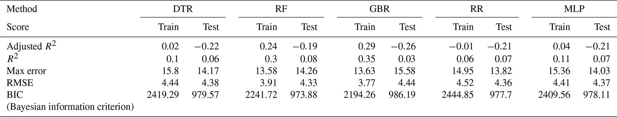
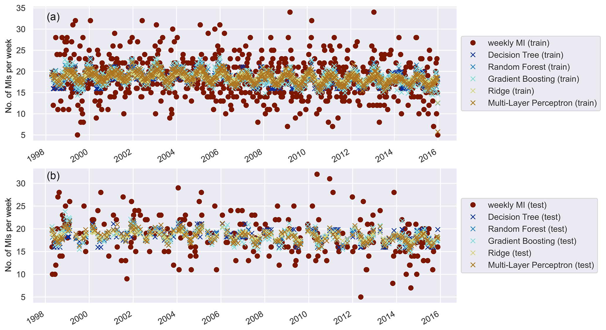
Figure 3 Daily predictions aggregated to 7 d intervals for all models. Shows predicted (crossed) and observed MI (dotted) for the training (a) and test (b) sets.

3.5 Demographics

The absolute number of MIs depends not only on various environmental risk factors but also on the size and characteristics of the population. Disregarding other factors, any change in the absolute number of inhabitants would produce a similar change in the number of cases of MI as well. Moreover, both age and sex are strongly correlated with health outcomes in general, and specifically so for MI. Given trends of increasing urbanisation, rural depopulation and an ageing society, it is important to account for changes in both number of inhabitants and age stratification of the population over time. In addition, domestic migration reflected in relative changes between urban and rural parts, leading to differential changes in exposure to environmental hazards in the Augsburg region, can be important as well. We collected data from the Bavarian Office of Statistics that comprise annual values for the total number of inhabitants for each of the three counties, as well as the distribution of sex and age in the population from 1985 to 2015. Overall, 17 different age groups are accounted for as listed in Table 3. Since the algorithms require daily input values, a linear interpolation was applied to estimate the development within a given year.

4 Results

4.1 Weekly predictions of MI events

Our models produce daily predictions of MI events based on the environmental and demographic features within the given window size. We found that the models are not able to reproduce the daily variability in MI with sufficient accuracy. As an example, we show the daily predictions aggregated to 7 d intervals to increase visibility in Fig. 3. The resultant scores are given in Table 4 for both training and validation, respectively.

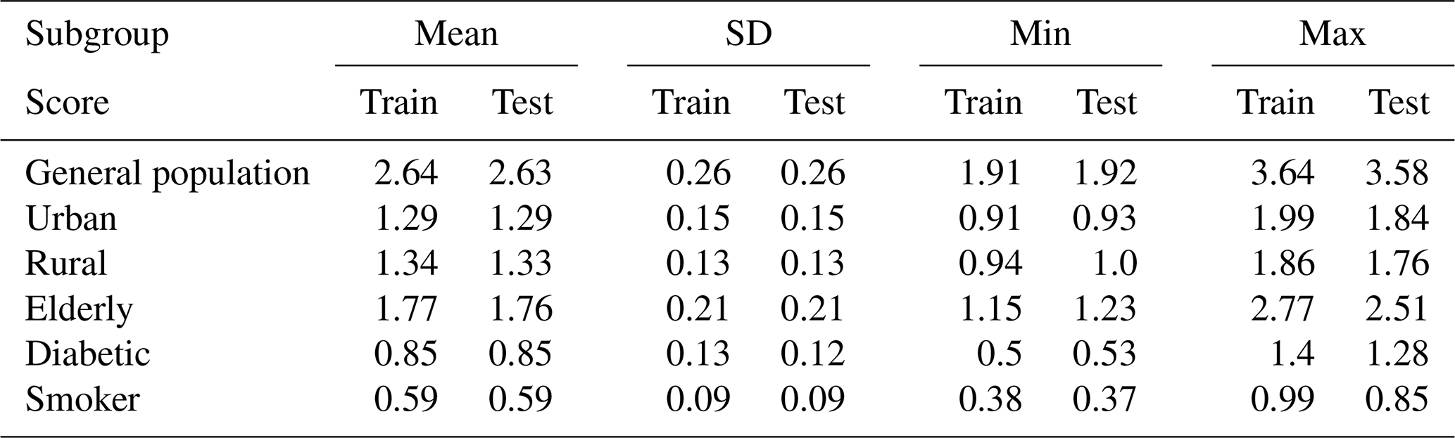
Although the 7 d predictions suggest some skill for the training period, for the testing period the models do not predict 7 d variations (or day-to-day predictions) accurately enough for practical purposes. The predictions are too close to the mean and lack the variability displayed by the observations. An overview of average mean, standard deviation, and minimum and maximum daily predictions across models and for each subgroup considered is given in Table A8. This is likely related to randomness as well as risk factors that affect MI events that were not considered in the models. For instance, the temperature or air quality predictors may not sufficiently capture actual local circumstances, but also information about the built environment and other conditions that cannot be easily accounted for is missing.

Table 5 Training and test scores on annual basis for the general population.

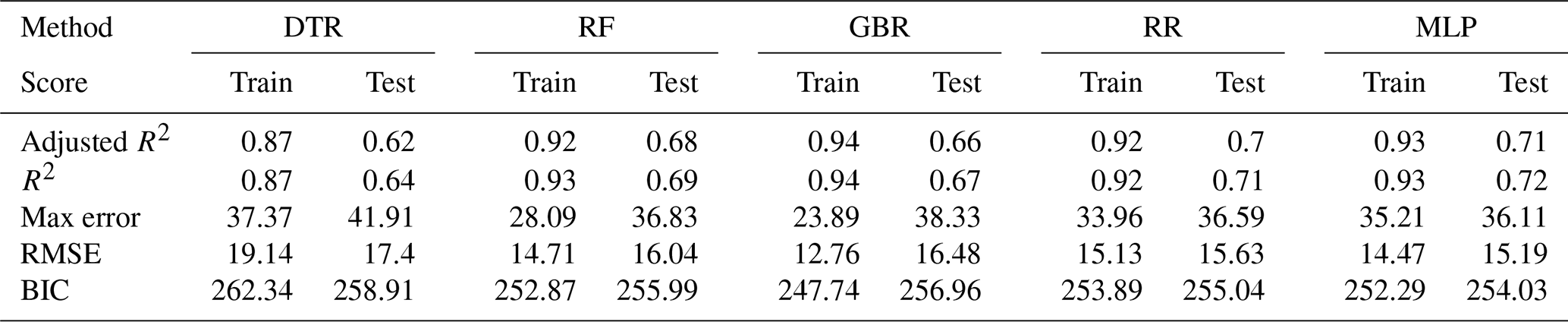
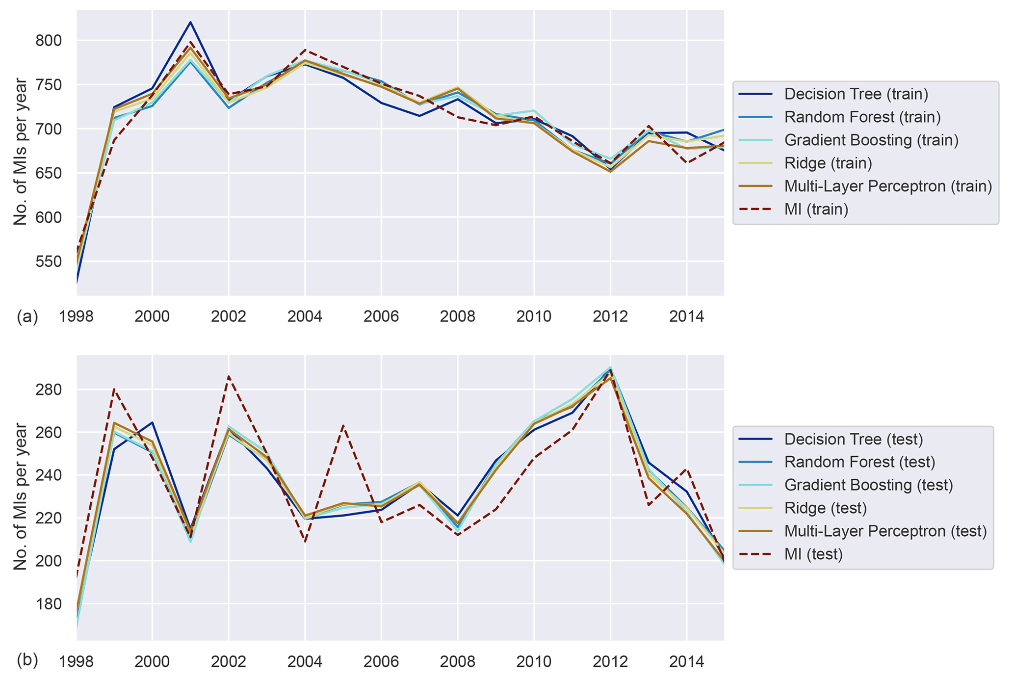
Figure 4 Annually aggregated predictions of MI in the general population for all models. Predicted (solid) and observed MI (dashed) for training (a) and test (b) sets.

4.2 Annual predictions of MI events

Figure 4 shows the model performances on both the training and test sets as well as the actually observed MI as a reference for the five ML models given in Table 1. After training the models and performing the daily prediction on the test set, the results were aggregated to annual sums. By aggregating the model results to an annual basis, some of the inherent randomness is averaged out. Based on the annualised prediction results and time series of observed MI, the performance scores were derived (see Table 5). The training scores demonstrate that the ML models are able to predict the year-to-year variations quite well, with adjusted R² scores between 0.87 and 0.94. The performance on the test dataset is relevant for assessing the generalisation error for previously unseen data. In contrast to the training data, the results on the test set are less but still reasonably accurate, with adjusted R² scores between 0.62 and 0.71, showing that inter-annual variations and long-term trends are largely captured. The RR and MLP models exhibit the best performance, showing that both well-tuned linear models and neural networks are able to simulate the relations between environmental conditions and MI events. The DTR shows the lowest overall performance by comparison.

4.3 Feature importance

In Fig. 5 we show a condensed rendition of the feature importance, where related variables have been grouped together for each model, except for the MLP, which does not support feature importance within the scikit-learn framework. Note that variables subject to the sliding window were aggregated over the window length of 3 d to improve readability. Moreover, features related to time such as the current month number and the day of the week were also aggregated to a single group. More detailed plots retaining the differentiation of all features and window days can be found in the Appendix (see Figs. A6 and A7). The latter figure also shows that many of the original demographic features carry little to no weight. We therefore reduced the granularity of the demographic data to the age groups 0–29, 30–49, 50–74 and >75, generally yielding improved results.

Figure 5 Aggregated feature importance for predicting MI for the general population. Related features have been grouped thematically. Larger values indicate higher importance, and per model the sum over all features equals 1.

While the performance of the models differs, some trends can be observed. Overall, the single most important group is air quality, closely followed by temperature-, demographic- and time-related predictors. Humidity as well as NDVI exhibits the lowest explanatory power. NDVI is ranked very closely to the random feature by all models.

Compared to the environmental features that display strong daily variation the demographic predictors are subject to slow, gradual change only. We therefore also conducted this experiment with all demographic features turned off. The results are shown in Table A7. As evidenced by the reduction in scores (adjusted R² reduced from 0.67 to 0.62 on average) the demographic predictors still make a relevant contribution to the overall result despite the lower temporal resolution of the input data.

4.4 Subgroup analysis

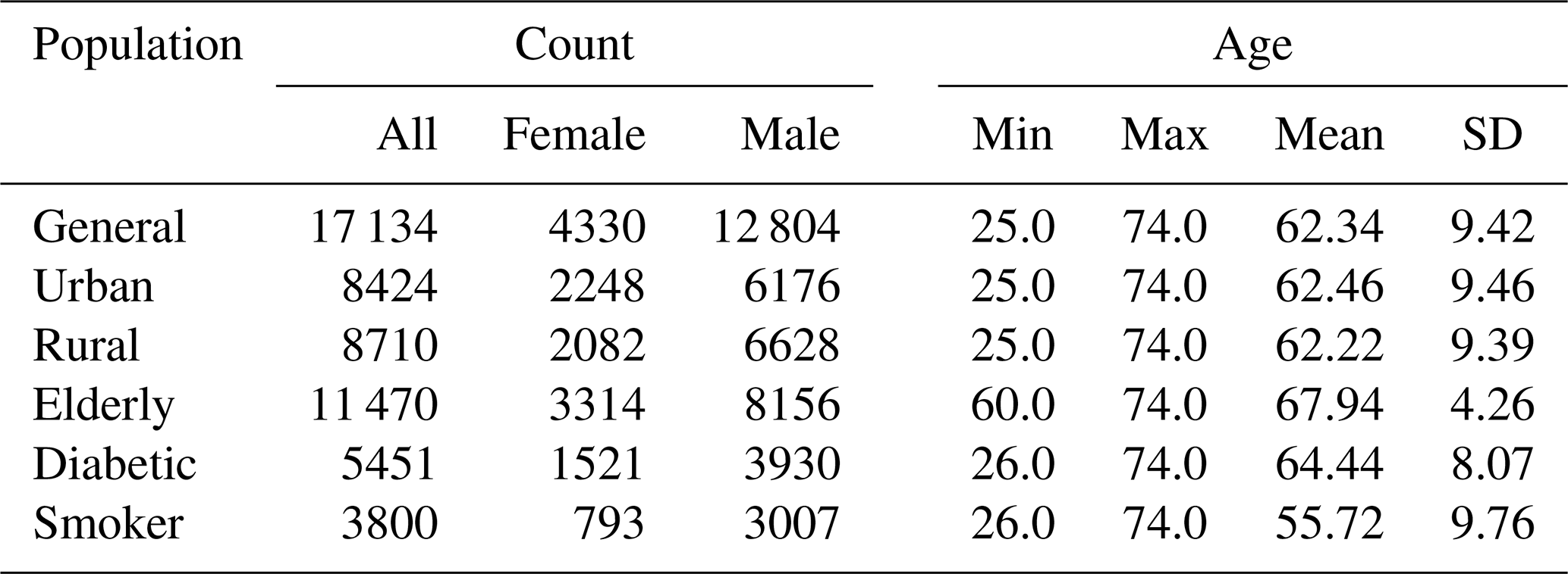
The models were also applied to subgroups of the population, albeit at the expense of a reduced number of available training data (see Table 6 for an overview). For this analysis we selected a total of five subgroups: the urban (Augsburg city) and rural population (two adjacent counties), respectively; the elderly (people aged between 60 and 74); patients with diabetes; and active smokers. The data were reduced to include only participants with the associated attribute. The training procedure was then repeated as detailed for the general case on the resulting subsets. As expected, the validation scores dropped considerably for all subgroups, likely a consequence of reduced quantities of training data. We refer to the Appendix for detailed results, but for the urban and rural subgroups adjusted R² scores between 0.35 and 0.6 were observed in validation (see Tables A2 and A3). Both subgroups, being of almost equal size, performed comparably well, with the urban population exhibiting slightly lower scores however.

Table 6 Overview of the number of cases as well as age and sex distribution for the different study populations considered.

The validation results for the elderly population (see Fig. A3 and Table A4) are more accurate (adjusted R² between 0.53 and 0.65) than for the urban and rural populations, although the number of training samples is much higher in both of those cases.

The results for patients with diabetes are shown in Fig. A4 and Table A5. As observed with the elderly, the scores for patients with diabetes (adjusted R² between 0.28 and 0.61) are comparable to those of the (much bigger) rural and urban subgroups, except for DTR, which resulted in a substantially reduced score.

The results for the smoking population are shown in Fig. A5, and the scores are given in Table A6. For this group adjusted R² validation scores drop to around 0.42 on average, indicating a less accurate fit than for all the other subgroups. This is consistent with the smoker group being the smallest of the explored subgroups, resulting in the lowest number of training data as well.

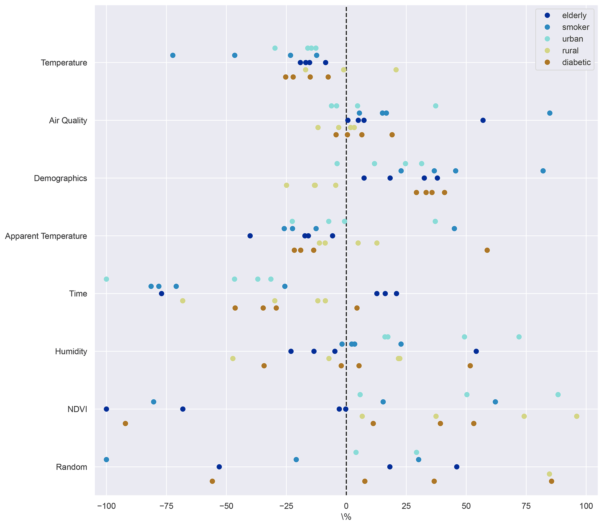
Figure 6 Change in feature importance for predicting MI in percent relative to the general population for every subgroup considered. Related features have been grouped thematically.

Overall, the skill of the models is clearly reduced when limited to subsets of the overall data. The decrease in performance, however, is quite different between subgroups, especially when taking into account their relative sizes. A particularly interesting question is whether the variable importance for any one subgroup changes substantially in comparison to the general population. Figure 6 shows the difference in variable importance for each of the subgroups in relation to that of the general population. To aid readability, related features have been grouped again. Considerable differences between subgroups, models and feature groups can be observed. For instance, most models agree that demographics, humidity and NDVI are particularly important for predicting urban MI while giving less weight to the temperature-related features. The importance of time-related indicators reduced consistently over the general population. In some cases the importance of the random feature is also reduced, indicating increased robustness of the results.

For the rural population the results suggest slightly increased relevance of NDVI compared to the overall population. Temperature and air quality mostly align with the results for the general population. The demographic indicators are less relevant when compared to the general case, as are the time-related features.

For the elderly, the models are mostly undecided on air quality, with a slight tendency towards increased importance. The weight of the demographic features is emphasised in comparison to the general case. Less importance is also attributed to (apparent) temperature and humidity.

For patients with diabetes, the models mostly agree that demographic features, NDVI and air quality are more important in predicting MI for this group in comparison to the general population. On the other hand, (apparent) temperature-, humidity- and time-related features are ranked lower.

Lastly, for the group of active smokers the models mostly suggest an increased importance of air quality as well as demographic features for the prediction of MI. Humidity as well as (apparent) temperature- and time-related features is overall considered less important.

5 Discussion

To our knowledge, this is the first study building and testing ML models that include more than only weather variables (such as Zhang et al., 2009, for heat mortality) for predicting MI prevalence. The developed ML models have varying skill in predicting MI. At the daily to 7 d timescales, randomness seems too large to produce meaningful predictions. However, when predictions are aggregated to annual sums, the models are very well capable of reproducing the inter-annual variability in observed MI, as well as the long-term trends, also for the validation datasets. This is comparable to the performance of methods used for predicting malaria incidence (e.g. Sewe et al., 2017). In terms of performance scores the models achieve very similar outcomes in both training and validation (see Table 5), indicating some robustness of the predictions. More qualitative differences emerge, however, when investigating feature importance. There are substantial differences between the ML models in terms of some features (Fig. 5). Most models rank air quality variations and temperatures among the most important features, but a large spread between models can be observed. This indicates at least some inherent uncertainty.

Classical epidemiological approaches like general linear or additive models are mostly used for explaining the direction and corresponding uncertainty in associations between environmental risk factors and health outcomes, thereby adjusting for potential confounding factors. In the case of potential non-linearities, the shape of the exposure–response curve is usually modelled as a smooth function. However, the models are limited in the case of high correlation and/or high-dimensional interactions between the covariates. The suggested ML approaches can (partly) handle these issues and offer the possibility of comparing the importance and predictive performance of a multitude of environmental predictors.

The training scores in many cases are close to the maximum, with adjusted R² values greater than 0.85. This may be indicative of overfitting, possibly opening room for improving further on the generalisation by applying stronger regularisation. While the models were adjusted by optimising the hyperparameters, not all possible parameter values have been explored. For instance, in the case of the tree-based models pruning is an effective way to reduce overfitting, which was not applied here. For the MLP and RR models regularising parameters were explicitly included in the optimisation, but possibly the ranges were not wide enough to achieve the best trade-off between training and validation.

The model results are sensitive to the selection of the random seed that is used in making the initial train–test split. We found that changes in the random seed routinely had greater impact than the choice of hyperparameters. One way of dealing with this would be to also include this random seed in the optimisation process. Currently, only the random seeds used for randomly selecting the folds in cross-validation and in initialising the regressors are optimised. In light of the strong influence of the initial split, however, we opted to instead test over a range of possible seeds and select the results closest to the average performance of the models, not to overstate our results. The sensitivity to the initial split may indicate a lack of data but is likely mostly due to unbalanced splits. We reduced this sensitivity by employing a simple but effective stratification strategy. This reduced the variation across seeds but does not entirely resolve the issue. Possibly, more intricate stratification approaches may reduce the dependency even further.

We were able to indicate differences between different geographical regions, i.e. urban and rural populations. For instance, humidity, demographics and NDVI become more important predictors for the urban population, compared to the overall population, at the expense of (apparent) temperature. The models could be further improved by increasing the spatial representation, as the environmental predictors also would support this. Increased spatial representation would also allow for additional exposure metrics to be established and more predictors, such as those related to building structures, their insulation and energy efficiency.

An additional area of possible improvement is the environmental data. Some variables such as the NDVI and the air quality indicators were not fully available for the period between 1985 and 2015, effectively limiting analysis to the period from 1998 to 2015. It is also possible to reduce the bias in the station data (temperature, air quality), for instance by using more sophisticated interpolation methods or additional data sources such as from remote sensing.

All ML models' results consistently demonstrated the importance of the air quality variables. Climate impact studies, especially related to MI, might therefore benefit from carefully analysing possible future developments of these variables. Electrification of traffic, reduction in fossil fuel and related changes might yield substantial improvements in air quality in the future. Instead of just focusing on projected changes in, for example, temperature and humidity, scenarios for air quality need to be considered as well.

Current data availability from climate modelling and demographic and environmental scenario development provide many opportunities to use the developed ML models from our research for projecting future health risks. Ensembles of regional climate models provide climate projections with the highest spatial resolution. For the study region, EURO-CORDEX simulations (Jacob et al., 2014, 2020) can be considered, providing the largest ensemble of climate simulations at high spatial (0.11^∘, i.e. 12 km) and temporal (daily) resolution available today. Several of the predictors used in this study could be derived from the EURO-CORDEX ensemble, namely temperatures and in many cases relative humidity, as well as dew point temperatures. Alternatively, an ensemble of convection permitting decadal regional climate simulations at ∼3 km, for both historic and future conditions, has been created within CORDEX FPS (e.g. Ban et al., 2021). Using an ensemble of near-future (2035–2065) climate model simulations allows for scenario uncertainty, internal climate variability and climate model uncertainty to be assessed (Hawkins and Sutton, 2011) when comparing the changes in MI to the reference historical simulations.

Demographic predictions until 2039 for the study region at the county level can be obtained from the Bayerisches Landesamt für Statistik (2022). Longer-term projections up until the year 2060, albeit contingent on different socio-economic scenarios and at the level of the federal state of Bavaria, could be obtained from the Statistisches Bundesamt (2022) and be used to estimate the local projected demographics in the study area. These projections would provide a robust basis to estimate potential developments of the local population in the near-future.

For vegetation changes, as represented by NDVI, it can be reasonably assumed that the potential for increased greenness in the inner city is limited. Likewise, the potential for substantial effects from added green in the rural surroundings of Augsburg is low, as it is already ubiquitous there. We therefore believe that moderate up- or downscaling of NDVI patterns observed in the past and present may suffice to yield suitable estimates of possible future developments, such as adaptation measures of increasing vegetation to reduce the urban heat island effect.

Air quality projections are related to the emission scenarios used by global climate models. For the CMIP6 climate models, estimates of regional surface air quality are available at the global model scale (Turnock et al., 2020). These projections could be used to scale the observed daily air quality observations, but more exhaustive and local projection data would be preferred. To date, however, regional climate models do not feature the necessary complex chemical models to accurately model the transport, dispersion and diffusion of pollutants. A pragmatic up- or downscaling of the observed patterns from the global to the local level currently appears to be the most convenient approach.

6 Conclusions

We have developed an approach for predicting MI events using multivariable ML methods, based on environmental and demographic data. Given that health outcomes depend on a multitude of factors, we applied a data-driven approach to establish relevant relationships. We acquired data on MI events from the KORA MI registry in Augsburg, Germany, as well as weather, environmental and demographic data from various sources to create a meaningful and consistent daily time series of the predictive features and the target variable.

Starting from these time series, a supervised learning problem for MI was formulated, accounting for lagged effects. Five different regression algorithms were trained on these data, based on random $\mathrm{75}/\mathrm{25}$ train–test splits for the period between April 1998 and December 2015. Various hyperparameters were used to optimise the performance of the algorithms, based on 5-fold cross-validation with respect to the R² scores.

Applying the trained models on the unseen test data allowed an estimation of the generalisation error of the models. We found that the daily or weekly results do not provide meaningful and accurate predictions of MI events. We found that the annually aggregated predictions agree well with the observed MI events, accurately reflecting observed trends and inter-annual variability in MI. The match between observations and the model predictions is supported by the observed validation scores, with adjusted R² scores ranging between 0.62 and 0.71. Overall, the models displayed comparable skill, but the ridge regression (RR) and multi-layer perceptron (MLP) models slightly outperformed the tree-based methods. The least accurate results were produced by the decision tree (DTR) model. The feature importance showed that despite similar overall scores, the relative weight can vary substantially between the models. This emphasised the necessity to consider ensembles of models, as it allows the model spread to be gauged and inherent uncertainty to be estimated. In this study, air quality tends to be the most important feature to predict MI, closely followed by temperature, demographics and apparent temperature. We also applied the models to various vulnerable subgroups, such as the elderly or patients with diabetes, resulting in only slightly reduced skill scores due to the reduced quantities of training data.

Possibilities of improving the current approach are manifold, including increasing the variety and quality of the predictor data. Further analysis of the data, including accounting for trends over time, may further increase robustness of the results to prevent the attribution of exogenous effects not considered in the model to the existing features. Also, different ML approaches could be explored, such as density estimation and Bayesian methods, yielding estimates of relative risk of different groups to suffer MI. Such estimates could be more readily compared with commonly used epidemiological models than the regression models presented here. Overall, the models' capacity to give reasonable estimates of possible future developments of MI based on the predictive features appears robust. In a next step, the trained models can be applied to scenarios of future climatic, environmental and demographic conditions. This will allow the estimation of future changes in MI taking into account climatic as well as other environmental and demographic factors expanding on limitations of earlier studies. These changes could also include further improvements in air quality or increased “greening” of urban environments with vegetation. Such estimates will enable the gauging of the sensitivity of the complex health–environment interactions and benefits of proposed environmental and health interventions in urban areas.

Appendix A

A1 Derivation of apparent temperature

We have computed the apparent temperature according to

$$\begin{array}{}\text{(A1)}& T_{\mathrm{a}}=-\mathrm{2.653}+\mathrm{0.994}T+\mathrm{0.01537}{T}_{\mathrm{d}}^{\mathrm{2}},\end{array}$$

where T_a is the apparent temperature, T the near-surface mean temperature and T_d the near-surface dew point temperature (see Davis et al., 2016). Dew point temperature, however, was not available for this study. To facilitate the estimation of the apparent temperature we therefore first derived another humidity-related quantity: vapour pressure. Applying again universal Kriging with linear drift, we arrived at 1×1 km gridded data for vapour pressure, applying the Magnus formula to estimate the dew point temperature:

$$\begin{array}{}\text{(A2)}& T_{\mathrm{d}}={\displaystyle \frac{b\cdot v}{a-v}},\end{array}$$

where a=7.5; b=237.3; and $v={\log }_{\mathrm{10}}\left(\frac{p_{\mathrm{v}}}{\mathrm{6.1078}}\right)$, with p_v the vapour pressure.

Applying these formulas to the gridded temperature and humidity data derived before yields a 1×1 km grid for apparent temperature. Note that the formulas were independently applied to mean, maximum and minimum temperature. Subsequent aggregation over the model region then completed the preparation of apparent temperature as an input feature.

A2 Detailed subgroup and feature importance results

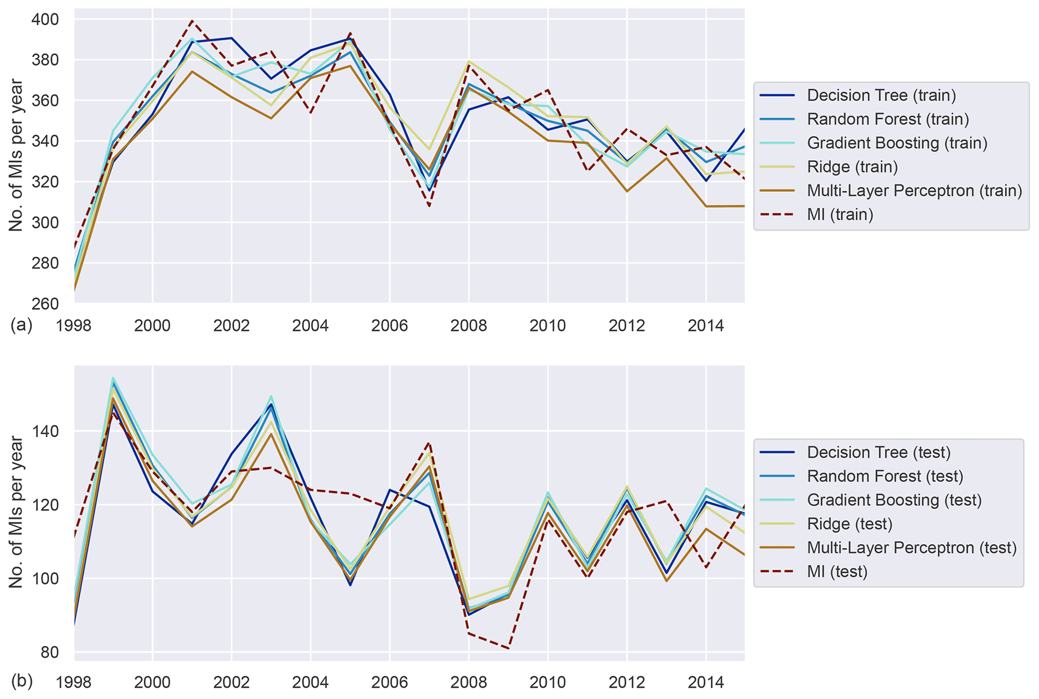
Figure A1 Annually aggregated predictions of MI in the urban population for all models. Predicted (solid) and observed MI (dashed) for training (a) and test (b) sets.

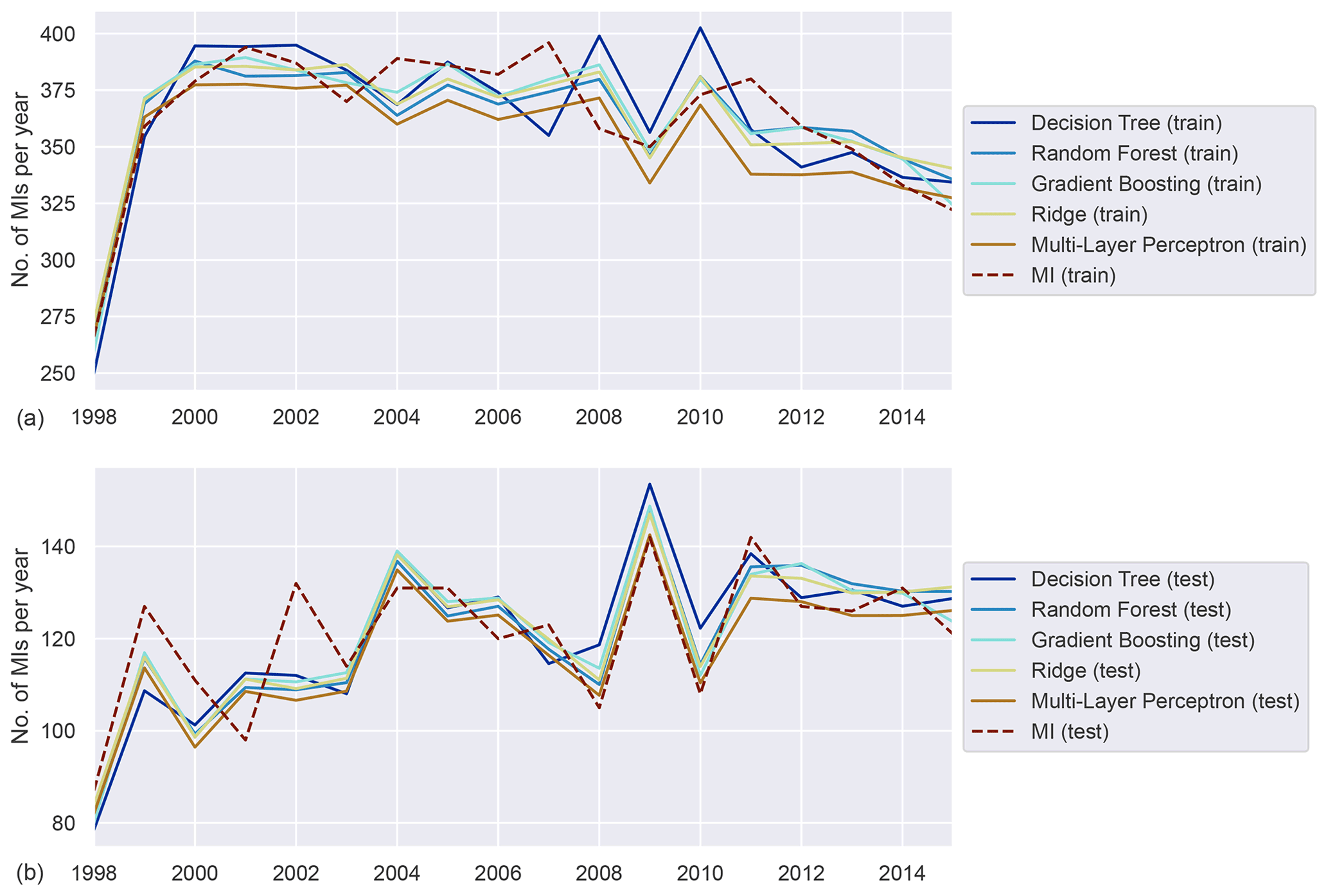
Figure A2 Annually aggregated predictions of MI in the rural population for all models. Predicted (solid) and observed MI (dashed) for training (a) and test (b) sets.

Figure A3 Annually aggregated predictions of MI in the elderly population for all models. Predicted (solid) and observed MI (dashed) for training (a) and test (b) sets.

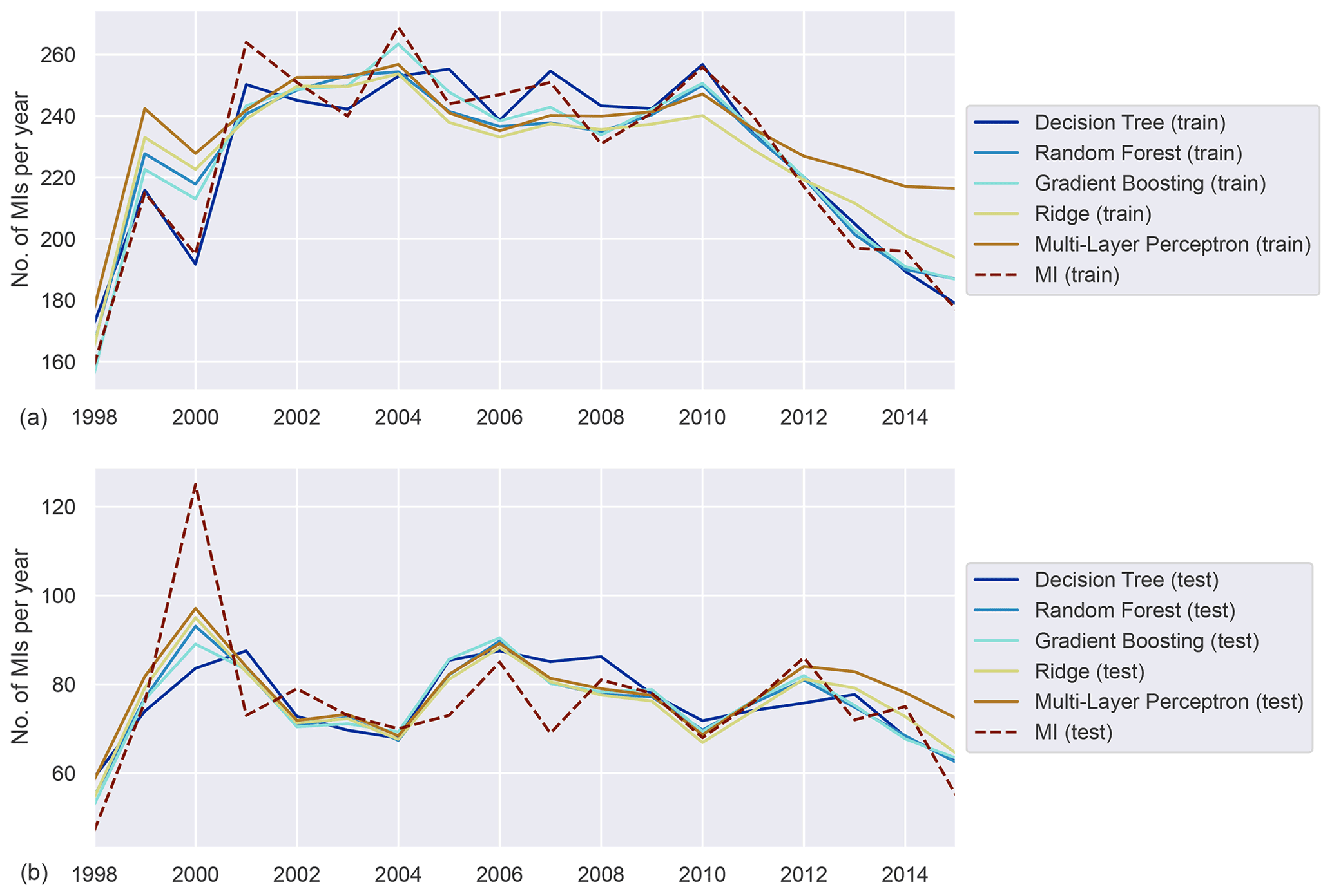
Figure A4 Annually aggregated predictions of MI in the diabetic population for all models. Predicted (solid) and observed MI (dashed) for training (a) and test (b) sets.

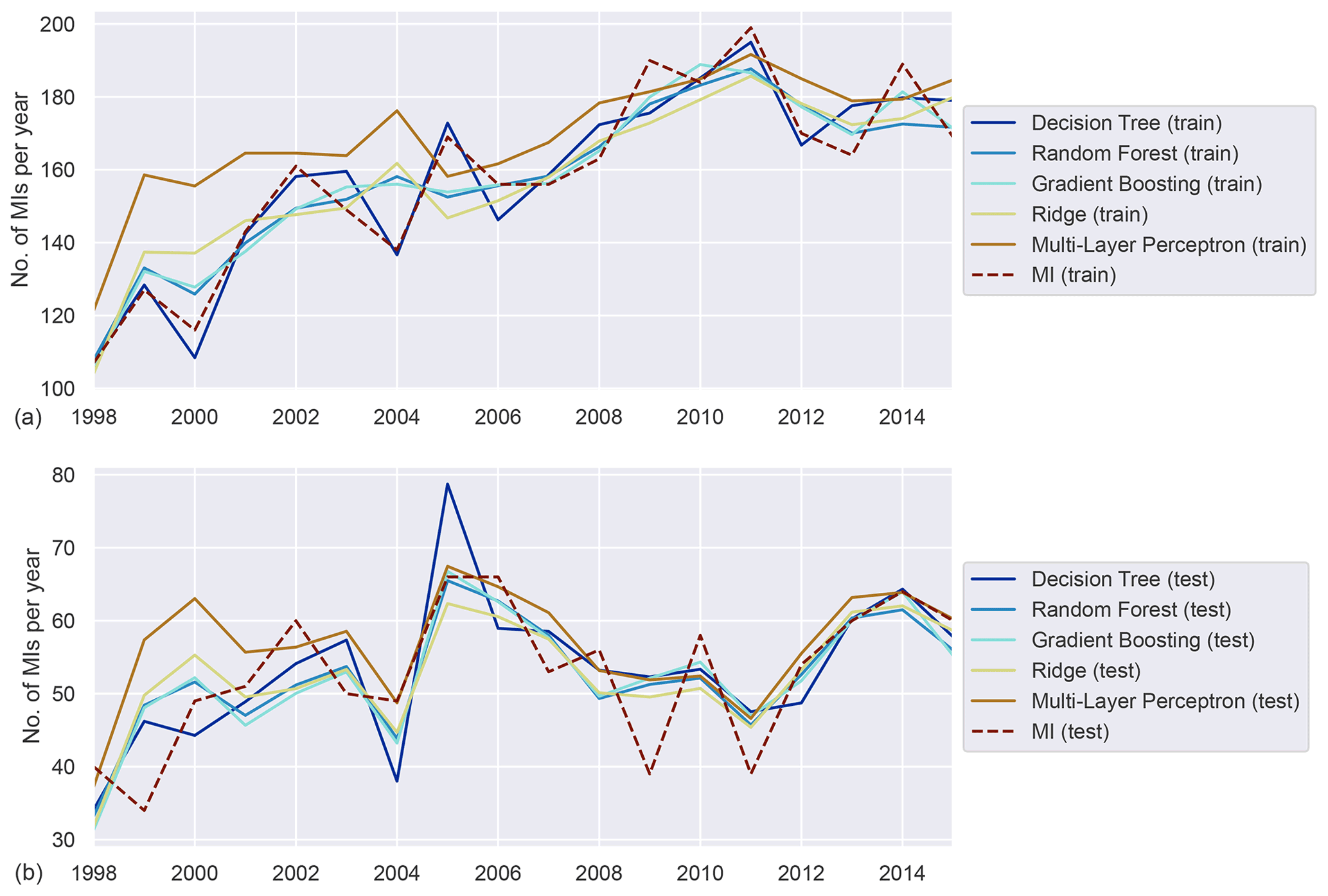
Figure A5 Annually aggregated predictions of MI in the smoking population for all models. Predicted (solid) and observed MI (dashed) for training (a) and test (b) sets.

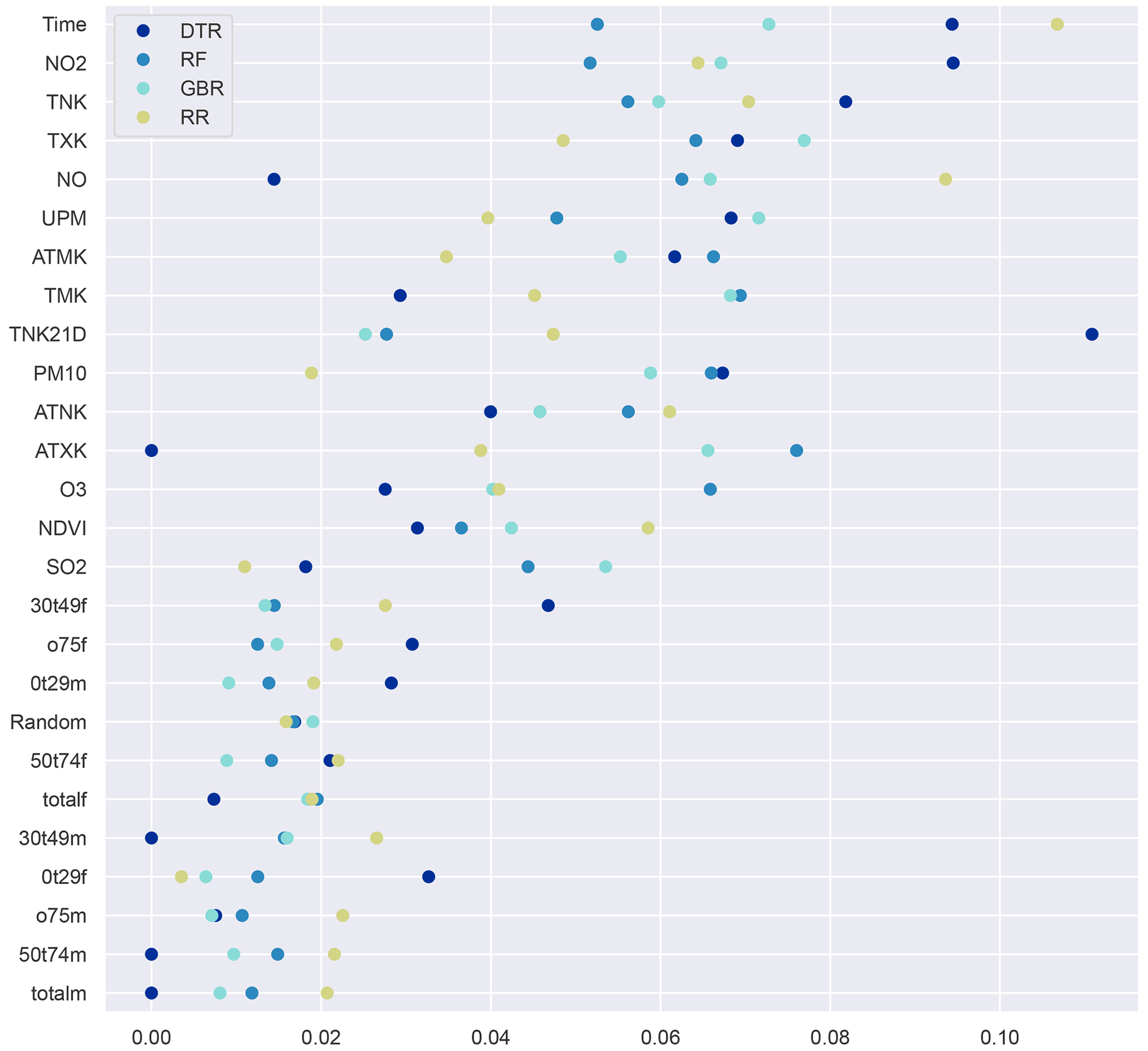
Figure A6 Feature importance for predicting MI in the general population. Larger values indicate higher importance, and per model the sum over all features equals 1.

Figure A7 Feature importance for predicting MI in the general population when the full set of demographic features is used. Where applicable the lag in days (0, 1 or 2) is indicated. Larger values indicate higher importance, and per model the sum over all features equals 1.

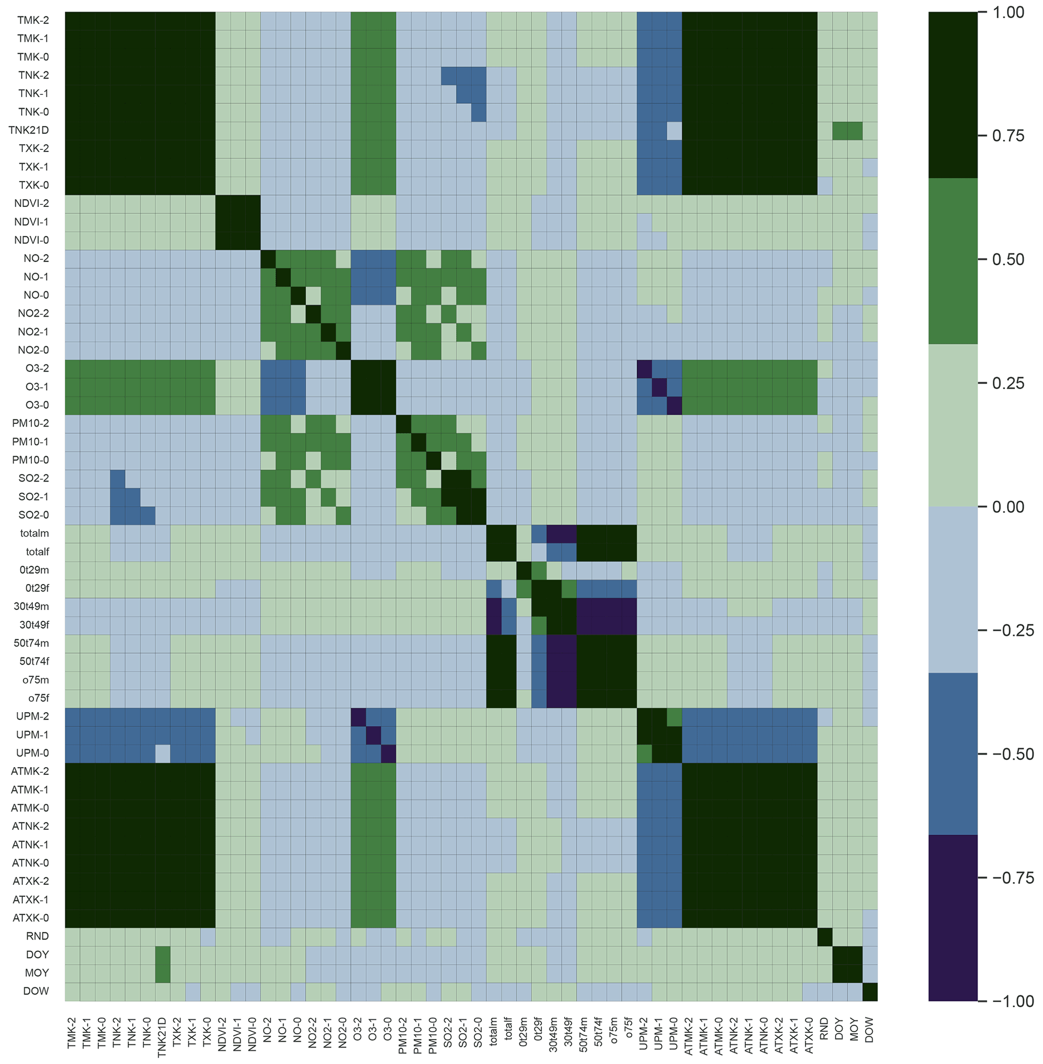
Figure A8 Feature correlation matrix differentiated by lag in days (0, 1 or 2) and with the full set of demographic features.

Figure A9 Monthly mean time series for all air quality features.

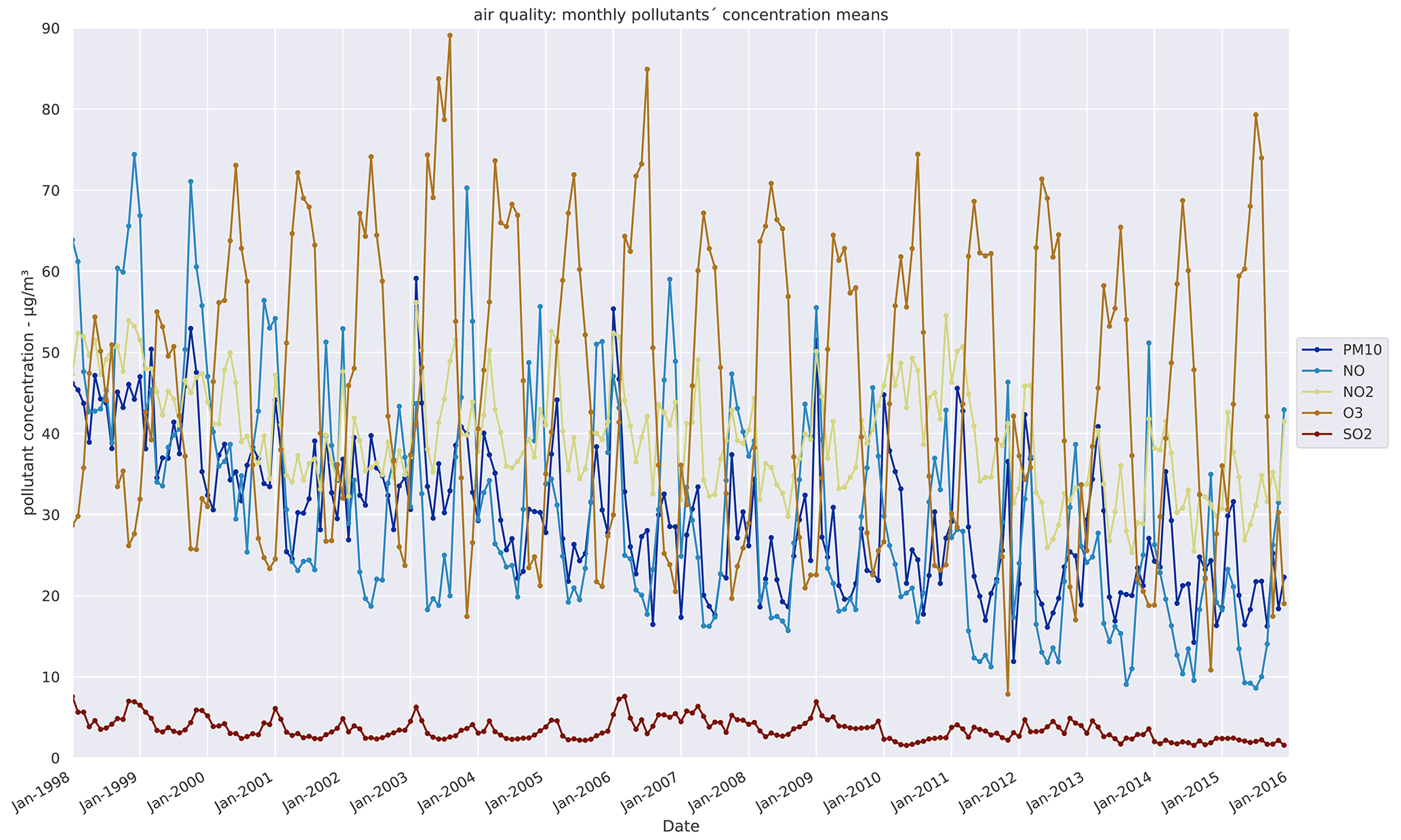
Table A1 Air quality stations data availability and categories.

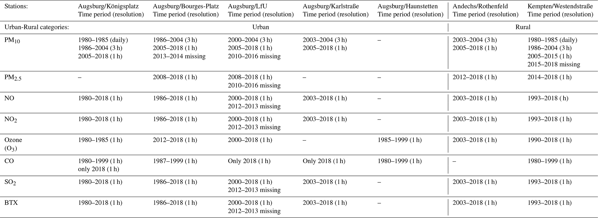
Table A2 Training and test scores on annual basis for the urban population.

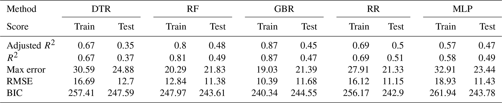
Table A3 Training and test scores on annual basis for the rural population.

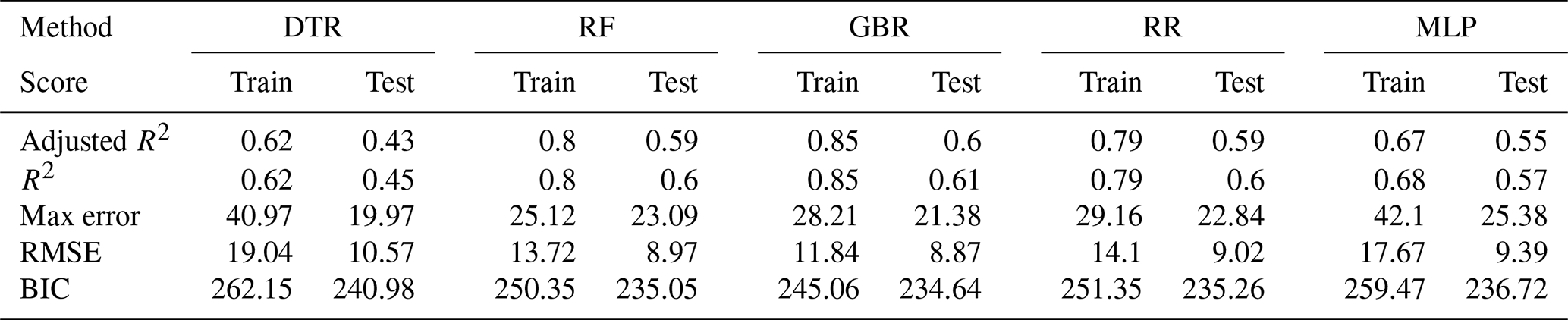
Table A4 Training and test scores on annual basis for the elderly population.

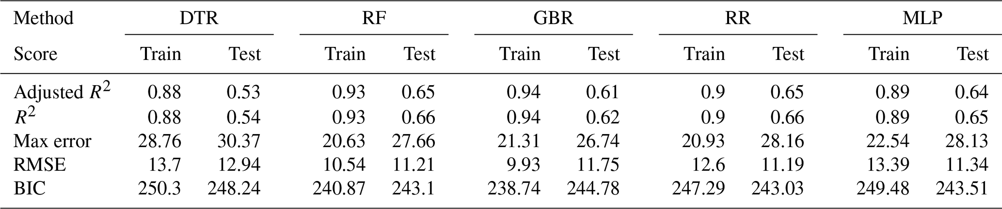
Table A5 Training and test scores on annual basis for the diabetic population.

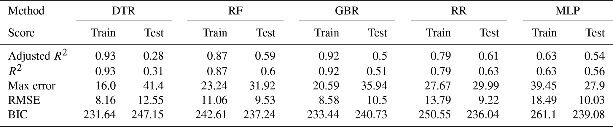
Table A6 Training and test scores on annual basis for the smoker population.

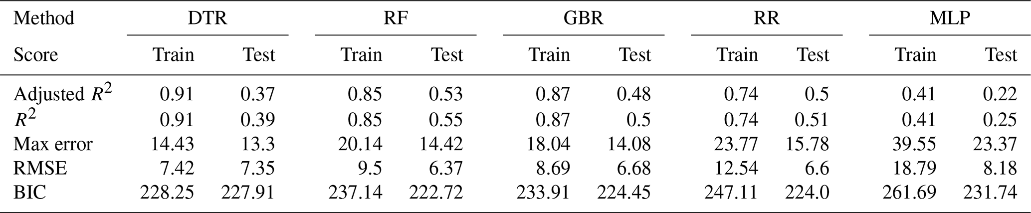
Table A7 Training and test scores on annual basis for the general population with demographic features turned off.

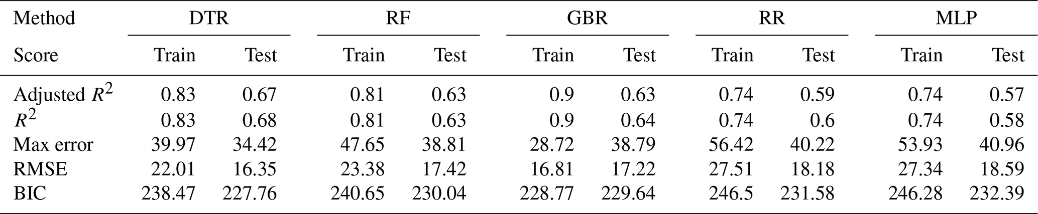
Table A8 Daily mean, standard deviation, and minimum and maximum predictions across models for each subgroup.