Assessing flood hazard changes using climate model forcing

A modelling framework for using regional climate projections to assess flooding hazard has been developed and applied to the Gwydir River (catchment 26 600 km² and floodplain 8100 km²), NSW, Australia. The model framework uses NSW and ACT Regional Climate Modelling version 1.5 projections combined with computationally efficient hydrologic and hydraulic models. Although it required model management and high-performance computing resources, the modelling framework successfully processed 18 regional climate projections into flood projections. Specifically, a six-member set of climate model combinations simulating a historical period (1951–2005) and a future period (2006–2100) under two global emission pathways (RCP4.5 and RP8.5) were used to predict flood depth and speed. In total, 1470 continuous years were simulated at hourly time steps. These flood (depth and speed) projections were analysed to assess the flood hazard changes under future climate scenarios by estimating changes in the annual probability of occurrence of a range of flood hazard classes. The six-member ensemble indicates that the flood hazard in the Gwydir Valley will decrease in the short, medium and long term. There are also cases within the ensemble, which includes increases in all non-safe flood hazard classifications while decreasing the safe flood hazard classification.

1 Introduction

Climate change potentially includes changes in temperature, evaporation, rainfall, and their seasonal patterns. Changes in rainfall patterns translate to changes in flooding extent, duration, and strength (i.e. flood hazard). Preparing for potential future changes in flood hazard can require significant lead times; thus, it is critical to incorporate climate change information into flood hazard risk assessment and adaptation planning. One way of investigating the nature of potential future flooding involves climate model outputs being converted to hydrodynamic outputs (flow depth and speed as a function of time), but this is not a trivial task and there is no general agreement on an approach. For example, future climate-related changes in the fitted distributions to channel discharge estimates have been evaluated using stochastic methods, water balance modelling and change factors (Delgado et al., 2014; Hirabayashi et al., 2013; Smith et al., 2014a). On the other hand, the direct application of climate model outputs has been discouraged by some (Cloke et al., 2013; Prudhomme et al., 2010). Nevertheless, some accelerated models for converting discharge into floodplain inundation show promise for converting regional-scale climate model outputs into continuous flood dynamics for hazard assessment on large and complex floodplains (e.g. Bates et al., 2010; Falter et al., 2013; Ghimire et al., 2013; Lhomme et al., 2009).

Assessing the future flood hazard under climate change directly (i.e. from hazard = depth × speed) at regional or jurisdictional scales requires the ability to simulate river discharge and floodplain inundation at hourly (or better) time scales over many decades and across large areas. The necessary computational efficiency can potentially be achieved by a variety of physics-based approaches including dynamic wave, partial inertial wave, diffusive wave and kinematic wave models (e.g. Montanari et al., 2009; Bates et al., 2010; De Roo et al., 2000; Miller, 1984). These involve simplifying the physics that are simulated together with a reduction in detail for one or two of the flow dimensions. For example, the computationally efficient LISFLOOD-FP offers options to implement such as dynamic wave, partial inertial wave or kinematic wave depending on what the environment being modelled demands (Lhomme et al., 2010; Bates et al., 2010, 2005). Decisions are therefore required on which physical processes can safely be ignored in the river environment of interest. Alternatively, there are computationally efficient rules-based models that involve a set of rules that mimic continuity and kinematic limits (e.g. Guidolin et al., 2016). The best choice of these two model approaches for undertaking a flood hazard assessment under future climate change optimizes the trade-off between model accuracy and computational effort with obtaining the necessary flood outputs to calculate hazard.

Performing hazard risk assessments and developing adaptation strategies for hazards under future climate change generally requires regional-scale (or better) climate projections. This involves refinement of global climate models through either statistical down-scaling (e.g. Wilby et al., 1998; Schmidli et al., 2006; Timbal and Jones, 2008) or dynamical down-scaling (e.g. Laprise, 2008; Giorgi, 2006; Ekström et al., 2015). The Australian NSW and ACT Regional Climate Model (NARCliM) is one example of this approach and used dynamical downscaling of a global 50 km model grid to a regional 10 km model grid (Evans et al., 2014; Nishant et al., 2021). Climate models represent the distribution of weather and as such, comparisons between climate model projections and historical measurements are possible by comparing their distributions but not by comparing specific historical events. Comparing distributions requires a balance between a measurement and model record long enough for such distributions to be appropriately defined while being short enough to limit non-stationary impacts from the changing climate. For parameters such as daily temperature or average rainfall, a 20-year period is suitable given that there are many rainfall events per year and every day has a maximum temperature (near continuous variable). For parameters with rarer occurrences, such as floodplain inundation, defining their distribution becomes increasingly more marginal. For example, defining changes in flood inundation that is exceeded every 100 years using a 20-year simulation period comes with considerable uncertainty. However, we may be able to usefully compare relevant measurements and model projections for more frequent events, such as the annual flood hazard classes.

Recent work investigating projected changes in flood risk under plausible climate futures includes Shrestha and Lohpaisankrit (2017) who forced a rainfall runoff model to estimate changes in discharges in the streamwise direction, allowing evaluation of changes in future risk. Moreover, Janizadeh et al. (2021) trained a machine-learning model to convert basin geometry and rainfall into risk, which was used with climate projections to evaluate future risk changes. Finally, Ryu et al. (2022) analysed adjusted rainfall projections using flood frequency methods to assess risk changes at the basin level. The method here seeks to extend these by using a physics-based model to convert runoff into spatially explicit water surface levels and speeds across the entire floodplain and throughout the entire climate projection period. This objective overcomes issues around data-poor regions (i.e. where machine-learning methods are not possible), provides flood projections at consistent spatial and temporal resolutions across the full extents of the model (both streamwise and cross-stream), and permits application to river systems with complex hydraulics and discharge patterns (e.g. multiple and parallel channels), which rainfall-runoff models are unable to reasonably simulate.

The purpose of this paper is to describe the successful application of a modelling framework developed to convert climate model projections to hydrodynamic outputs, which were then used to assess future changes to present-day regional flood hazard. We demonstrate the utility of the approach by applying it to the Gwydir River, a large valley-floodplain system located in the northern Murray-Darling Basin, Australia. After reviewing candidate numerical models, a new method for driving a hydrological flow-routing model and the LISFLOOD-FP hydraulic model with climate projections for rainfall-runoff (or excess rainfall) was applied using the NARCliM1.5 climate projections, as an example. Rather than using the climate projections to determine key or design events for simulation, we simulate river floodplain hydraulics for the full climate projection time series. Projected future regional flood inundation extents and the spatial distribution of flood hazard are presented for two global emission pathways (RCP4.5 and RCP8.5). Challenges associated with spatial and temporal sparsity in floodplain inundation and applying conventional extreme value distributions to evaluate future flood exceedance probabilities are discussed. These confound efforts to answer the question – will present-day flood hazards change under future climate projections? We provide a new approach to answering that question.

2 Methods

The objectives in converting climate model outputs to inundation estimates were: (i) develop a method for manipulating NARCliM 1.5 hydrological variables for application in rainfall-runoff routing models that use rainfall minus the water that infiltrates the soil and is thus not available for runoff, (ii) review the literature to identify potential flood models suited to application over large spatial and temporal scales, and (iii) identify the most suitable flood model and apply to a large river valley. To successfully achieve these objectives, a series of principles were adopted to guide an iterative development of the model framework, which was then stress-tested on the Gwydir River floodplain, New South Wales (NSW), Australia. These principles, in no particular order are: (i) use NARCliM 1.5 outputs to force models suitable for flood inundation estimation; (ii) maximize benefit from inundation estimates by simulating the entire NARCliM 1.5 set of projections; (iii) use open datasets, methods, models and mostly automatic approaches; (iv) design the framework for implementation on high-performance computing resources; and (v) the historical period, constrained by measurements, determines parameter values applied to the forecast period. The modelling framework that achieves our aim (Fig. 1) and is consistent with these principles constrains both hydrologic and hydraulic models, takes boundary conditions from climate model outputs, simulates them entirely by breaking them into 4-year windows with a 2-month overlap for warming up the hydraulic model, develops initial conditions based on low flow conditions, simulated in parallel on high-performance computing resources and has data management to limit the file size associated with saving inundation depth and speed by storing the daily maximum inundated depth and associated flow speed. The various segments are then combined (removing the 2-month overlap) and stored in compressed netCDF files (https://doi.org/10.48610/d7b1654, Callaghan, 2022). The hydrologic and hydraulic methods used in this framework are discussed in Sect. 2.1 and 2.2.

Figure 1 Proposed framework for converting climate model outputs to flood model outputs.

2.1 Evaluation of climate model outputs and hydrological model theory

The NARCliM 1.5 climate model ensemble includes three global climate models (CCCma-CanESM2, CSIRO-BOM-ACCESS 1-0 and 1-3) with two regional climate models (UNSW-WRF360 J and K) resulting in a set of six model combinations (Nishant et al., 2021). Projections for two epochs (historical 1951 to 2005 and projections 2006 to 2100) using two global emission pathway scenarios (RCP 4.5 and 8.5) are available, and include hourly variables of precipitation and total run off, and bias-corrected daily precipitation (corrected to observed precipitation distribution; see for example Evans et al., 2021). Although NARCliM 1.0 selected CMIP3 GCMs, NARCliM 1.5 selected CMIP5 GCMs from the unsampled space within NARCliM 1.0, all with similar temperature increases but spanning the range of precipitation changes from no change to moderate decrease to large decrease (Nishant et al., 2021).

NARCliM 1.5 was applied by matching, as much as possible, measured and modelled climate statistics. For catchment runoff, this was done at Gravesend on the Gwydir River, where the measured distribution of annual maximum discharge was used to calibrate the hydrologic model. Gravesend (Fig. 2) is the last gauging station before the conversion between water level and river discharge becomes significantly uncertain (tailwater and inundation feedbacks leading to significant hysteresis). Each of the historical river discharge projections were calibrated using the measured distribution of annual maximum discharge at Gravesend. The hydrologic model used the excess precipitation (excess rainfall) obtained from NARCliM 1.5 (“total run off” code named mrro) in the following manner. The bias-corrected daily rainfall was used to bias correct daily total run off (or excess daily rainfall), and this was interpolated onto an hourly timeframe using the NARCliM 1.5 hourly precipitation for shape. That is

$$\begin{array}{}\text{(1)}& \begin{array}{rl}& \mathrm{daily}\mathrm{runoff}\mathrm{corrected}=\mathrm{daily}\mathrm{runoff}\\ & \times {\displaystyle \frac{\mathrm{bias}\mathrm{corrected}\mathrm{daily}\mathrm{precipitation}}{\mathrm{daily}\mathrm{precipitation}}}\end{array}\end{array}$$

and

$$\begin{array}{}\text{(2)}& \begin{array}{rl}& \mathrm{hourly}\mathrm{runoff}\mathrm{on}\mathrm{day}t=\mathrm{daily}\mathrm{runoff}\mathrm{corrected}\mathrm{on}\mathrm{day}t\\ & \times {\displaystyle \frac{\mathrm{hourly}\mathrm{rainfall}\mathrm{on}\mathrm{day}t}{\sum _{\mathrm{day}t}\mathrm{hourly}\mathrm{rainfal}\mathrm{on}\mathrm{day}t}}\end{array},\end{array}$$

where the last term in Eq. (2) ranges from zero to unity.

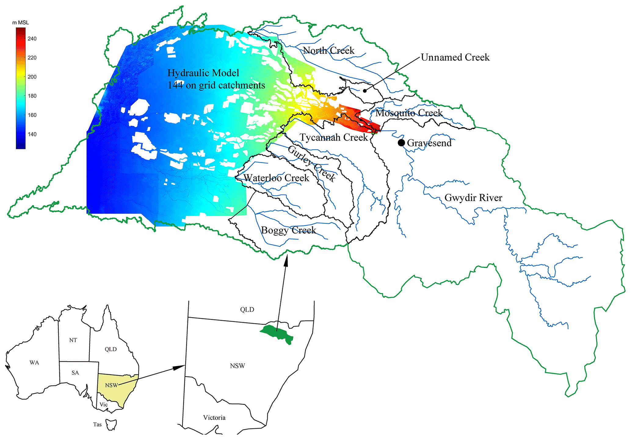
Figure 2 Catchments and waterways flowing through the Gwydir Valley with the location within New South Wales (NSW), Australia shown in the bottom left inserts. Hydraulic model extents shown by colour-shaded area representing ground elevation in metres above mean sea level (colour bar) with the main source of inflows from the Gwydir River, which has a gauging station at Gravesend (black dot). The 133 watershed boundaries within the hydraulic model and sub-catchments within each waterway are not shown for clarity. The white areas within the hydraulic model grid are areas surrounded by levees and are unavailable to convey water.

The excess precipitation was routed through catchment models following the method proposed by Mein et al. (1974), which is referred to as a ROR-style model with two free parameters, m and k, that are nominally for discharge shape and storage, but experience with this model indicates that their theoretical basis is weak and they are used as free calibration parameters. The external catchments draining to the hydraulic model (Fig. 2) come from Gwydir River, Boggy Creek, Waterloo Creek, Curley Creek, Tycannah Creek, Mosquito Creek, North Creek and an unnamed watershed. Each catchment was broken into between five and 13 sub-catchments, yielding an outflow suitable for use in the hydraulic model. The hydraulic model covers a significant area (9621 km²) and consequently, runoff onto the hydraulic model is included by associating sub-catchments with model grid locations. The climate projections have more than one grid cell within sub-catchments in many places, with these contributions reduced by the area of each cell from the climate projection overlaps each sub-catchment, with these contributions allocated in proportion to the grid cell overlap on the sub-catchment.

Comparisons with measurements of river discharge at Gravesend, on a distribution basis, indicated that using NARCliM 1.5 to provide excess rainfall and a ROR-style runoff routing model with no losses (initial or continuing) leads to overestimates of frequent events and underestimates of infrequent events. This indicates that there is not enough loss of water volume during lighter rainfall events compared with heavier rainfall events within NARCliM 1.5. There are many on-farm water storages not included in the NARCliM 1.5 or catchment hydrologic models used to this point. To include them, we extended the hydrology models by adjusting the excess precipitation before it is used for runoff routing. The excess precipitation was routed through a storage of maximum depth h_max, a surface area of fA (where A is the catchment area) whereas water within that storage was evaporated using a monthly mean of measured evaporation rates and a usage rate to model farm use. The storages were initially started at half full. If the storage does not overflow during a time step, there will be no excess rainfall. If the storage does overflow, then there will be excess rainfall, P_r, to yield runoff. Mathematically, if h is the depth of water in the storage, then it will change by

$$\begin{array}{}\text{(3)}& \mathrm{\Delta }hf=(P-(e+u\left)f\right)\times \mathrm{\Delta }t,\end{array}$$

where P is the NARCliM 1.5 excess precipitation, e and u are evaporation and usage rates and Δt is the time increment. This adjustment was applied as follows:

$$h\left(t\right)f+\mathrm{\Delta }hf>h_{\max }f\left\{\begin{array}{l}{P}_{\mathrm{r}}=\frac{fh+\mathrm{\Delta }hf-h_{\max }f}{\mathrm{\Delta }t}\\ h\left(t+\mathrm{\Delta }t\right)f=h_{\max }f\end{array},\right.$$

$$\mathrm{0}\le h\left(t\right)f+\mathrm{\Delta }hf\le h_{\max }f\left\{\begin{array}{l}{P}_{\mathrm{r}}=\mathrm{0}\\ h\left(t+\mathrm{\Delta }t\right)f=h\left(t\right)f+\mathrm{\Delta }hf\end{array},\right.$$

$$\begin{array}{}\text{(4)}& h\left(t\right)f+\mathrm{\Delta }hf<\mathrm{0}\left\{\begin{array}{l}{P}_{\mathrm{r}}=\mathrm{0}\\ h\left(t+\mathrm{\Delta }t\right)f=\mathrm{0}\end{array},\right.\end{array}$$

and if f=0, then the model simplifies to P_r=P.

2.2 Selection of hydraulic theory and code

Climate change evaluation at regional scale or larger for flooding hazard and other applications requires fast and accurate enough flood modelling. This review seeks to identify hydrodynamic models with proven track records to achieve this evaluation in a timely manner with limited human resources (automated processes). This assessment is separated into physics-based models and rules-based models.

Physics-based models typically follow Newton II and in particular, the shallow water equation or dynamic wave equation, applied in either one or two horizontal dimensions (e.g. 1D or 2DH), to solve for temporal and spatial variation in flow depth and speed. There are several well-known approximations of the dynamic wave equation, with kinematic, diffusive and partial inertial-wave (or long-wave) approximations possibly the best known. All physically based methods except dynamic wave exclude convective acceleration and hence, momentum changes required to change flow direction. Consequently, forces from water-surface gradients required to get flow through geometry changes (road embankments across a floodplain) is reduced when compared with including convective acceleration. These terms have been found to be essential in ocean models where mean water-level gradients are exceedingly small and flow mass exceedingly large (mean ocean depth is ca. 4 km).

There are too many examples of successful dynamic-wave application in two dimensions or a combination of one and two dimensions to list them all; however, the following subset (e.g. Montanari et al., 2009; Ahmadisharaf et al., 2018) highlight methods aimed at accelerating applications for flood management including graphics processing unit implementations through to careful use of 1D/2DH modelling (resulting in global-scale continuous simulations). This approach remains the benchmark theory for flood modelling.

Examples of successfully applied partial inertial wave models are numerous (e.g. Rajib et al., 2020; Sampson et al., 2015; Bates et al., 2010) and this approach has a proven track record of: statistical evaluations, hazard mapping or Monte Carlo risk evaluations including damage estimations with velocity and depth contributions (e.g. Hoch et al., 2017; Neal et al., 2013), large spatial and temporal scale assessments where channels were sub-grid features (O'Loughlin et al., 2020; Schumann et al., 2013), multi-channel assessments (Altenau et al., 2017), temporal scales from minutes to years (e.g. O'Loughlin et al., 2020; Neal et al., 2011) and on to geological scales (Coulthard et al., 2013), coastal storm surge inundation (Lewis et al., 2011), coastal tidal dynamics (Skinner et al., 2015), and flooding in urban, rural, remote and limited data applications (e.g. Amarnath et al., 2015; Bates et al., 2010; Fewtrell et al., 2011; O'Loughlin et al., 2020). Although there are notes of caution with this approach at large scale (Schumann et al., 2012) and other authors advocating for the diffusive wave (Dottori and Todini, 2013) over the partial inertial wave, it has the best track record after the dynamic-wave equation while being exceptionally quick. The partial inertial-wave equation has a theoretical limit in that at either high velocity (Froude number exceeding 1) or low frictional force, the momentum equation becomes unstable. This well-known issue has been noted in the recent literature with respect to LISFLOOD.

The diffusive wave equation has a long track record dating back to when hydraulic modelling using numerical methods in two dimensions started in the 1970's. However, in more recent times where it has been revisited for its light computing load (e.g. Mason et al., 2009; Apel et al., 2009; De Roo et al., 2000), it has been the reason for shifting to the partial-inertial wave equation (Neal et al., 2012), with only one reference found arguing diffusion over partial inertial wave (Dottori and Todini, 2013) for accelerated flood assessments. Further, there is evidence that a diffusive wave does not handle urban environments (Costabile et al., 2017) but away from these areas and with enhancements, it is accurate enough (Jamieson et al., 2012). The diffusive-wave model links forces to motion exclusively through the friction model whereas the partial inertia-wave model has a combination of friction and temporal acceleration. This fixed link through the adopted friction model means that uncertainties in the friction model and spatial and temporal parameter variations are more significant in diffusive-wave estimations. As the earlier engineers/scientists knew, applying diffusive wave theory to subcritical flow on a two-dimensional horizontal grid is often numerically unstable leading to the checkerboard predictions. Although some recent authors were seeking to address this numerical stability issue using careful spatial and temporal selections and flux gradient limiters, ultimately the decision to include the additional temporal acceleration (inertial) term resolved their numerical issues almost entirely. From the balance of evidence and theoretical arguments, it is proposed that the diffusive-wave model is an unacceptable approach when trading off between accuracy and speed.

The kinematic-wave equation has a long track record in modelling supercritical flows (Miller, 1984) with more limited application to subcritical flow modelling of prismatic channels (Zheng et al., 2020). When the continuity equation is combined with the kinematic-wave equation, predictions exclude flow attenuation and actually increase discharge and water surface slopes (Miller, 1984, p. 18). In the case of prismatic channels, the water depth and discharge are fixed or Q=Q(h), where Q is discharge (Henderson, 1966, p. 367) and yet numerical models of prismatic channels rarely achieve this and degrade to Q increasing with both time (t) and position. Miller (1984, p. 20) further indicates that for a successful kinematic-wave application, ad hoc modifications in how this equation is solved are required and then only on the rising limb. Consequently, large errors are expected when using the kinematic-wave equation in non-prismatic channel systems. The balance of evidence and theoretical arguments indicates that kinematic wave equation is an unacceptable approach when trading off between accuracy and speed.

The impact cell method is based on rules around how floodplains fill with water during flooding either over defences or by defence failure. They use a dynamic-wave equation one-dimensional model to drive the floodplain filling and although they appear to be temporal, they are quasi-steady (Lhomme et al., 2009; Gouldby et al., 2008; Hall et al., 2003). The major drawback is model development in that it involves a combination of physical and probabilistic inputs, which have no apparent automatic techniques for their estimation. There is a lack of a track record around estimating velocities from the water-level gradients that this style of model predicts.

The cellular automata method is based on a set of rules that mimic continuity and kinematic limits, which from limited testing (e.g. Jamali et al., 2019; Guidolin et al., 2016; Nicholas et al., 2006) is able to simulate urban areas, multi-channel systems and hydraulic structures within a gridded domain. Various versions do include storage attenuation. There is, however, no track record around estimating velocities from the water-level gradients that this style of model predicts.

There are other rules-based methods, including rating curve geographic information system models (e.g. Zheng et al., 2018; Apel et al., 2008) through to dynamic and rule-based combined models (Bernini and Franchini, 2013; Jamieson et al., 2012). These have not been considered as they exclude flow routing.

The trade-off between accuracy and computational effort and seeking flood hazard information thereby requiring reasonable flow speed estimates leads to the selection of the partial inertial-wave equation (LISFLOOD) and the cellular automata (WCAD2D). These two hydraulic models were compared in both steady and unsteady tests and evaluated for speed. Although estimates of flood levels from the two models were similar, LISFLOOD was found to be 2 to 2.5 times faster when tested on large floodplains such as the Gwydir River. This led to the selection of LISFLOOD.

2.3 Implementation of the LISFLOOD hydraulic model

The LISFLOOD model was limited to the region covering the Gwydir River Floodplain of 8100 km². LISFLOOD could have been applied across the entire catchment, removing the need for including a hydrology model. Although this may be useful in particular situations, for the present case study that would require a LISFLOOD model grid covering 2.8 times more area, unnecessarily increasing the burden on computational resources. Consequently, the ROR-style hydrology model with flow routing provides a trade-off between computational resources and framework complexity.

Surface roughness (using Manning's n) for the LISFLOOD model developed here was obtained from existing calibrated hydraulic models for the Gwydir River. There are three models forming the NSW Department of Planning and Environment Gwydir River hydraulic model with 1D links (channel links without hydraulic structures) and 2D grids with resolutions from 20 to 50 m using MIKE FLOOD (Anonymous, 2015). After balancing resolution with file size and run times, a 100 m resolution was selected. These three models were combined to develop the 100 m digital elevation model (DEM) with extents to enclose Binniguy to Moree, Moree to Barwon and Thalaba Creek MIKE FLOOD hydraulic models (colour-shaded area in Fig. 2). The origin was set so that the 100 m DEM collocated with every second grid point of the Moree to Barwon model. Crest features (usually roads, but any feature that could either act as a weir or a dam that changes discharge distributions) were extracted out of Binniguy to Moree, Moree to Barwon and Thalaba Creek DEMs, and put onto the 100 m DEM. This was achieved in a two-step process: first, a smooth version of each existing DEM was subtracted from the new 100 m DEM and differences below 0.2 m removed. The resulting features showed crests as well as other differences related to waterways. The crest features alignments were then determined, and the crests extracted. Waterways removed from Binniguy to Moree were put back in using survey DEM, missing areas were filled in using Shuttle Radar Topography Mission data and finally, streams were hydraulically connected (Fig. 2).

The three hydraulic models forming the Gwydir River hydraulic model by NSW government was used to constrain (to previously calibrated hydraulic models) the LISFLOOD model, using their 2012 calibration runs, performed in MIKE FLOOD. There are complications in that those NSW government models included 1D elements, had finer resolution (20 and 50 m) and were separated into three domains, one run in steady state (southern region) and the other two using dynamic simulations with varying simulation periods, compared with the one encompassing LISFLOOD model, which had a coarser resolution (100 m) and no 1D elements. To rationalize these comparisons, locations where the NSW government models had reported inundation were used to constrain the LISFLOOD model. The first calibration series ran 100 incremental model topographies from largest main channels possible from survey to no channels, and inflows taken directly from the NSW government models. The channel geometry was selected to obtain the best match to these calibrated models.

2.4 Climate projection to flood simulations

NARCliM 1.5 includes six historical projections and 12 future projections, providing 18 periods for simulation, covering a total physical time of 1470 years. The historical projections run from the start of 1951 to the end of 2005, which is 55 years each and a total of 330 years. The future projections from the start of 2006 to the end of 2100, which is 95 years each, total 1140 years. Consequently, the total from historical and future projections is 1470 years. Such simulations require high-performance resources and careful selection of outputs and model resolution to ensure that simulations are obtained within a reasonable timeframe. Within storage resources available, output from LISFLOOD was hourly and then post-processed to daily information of maximum inundation depth and the flow speed at that maximum depth. This, with several storage techniques to minimize file sizes (netCDF with compression and finite data resolution), reduced required storage from ca. 10 TB to 100 GB. Applications involving steeper catchments and floodplains may warrant storage of hourly rather than daily outputs. To further enhance model throughput, simulations were broken into 4-year segments, with an additional 2-month warm-up period using initial conditions taken from a low-flow simulation developed from measurements and average evaporation. It was confirmed that the 2-month warm-up period did not have an impact on projections by comparing projections from the end of a segment with the projections (after warm-up) at the start of the following segment. The model grid was selected after initial testing of four resolutions of 50, 75, 100 and 150 m. These tests indicated that simulation times, from finest to coarsest grids, were 55, 16, 7 and 2.5 d per decade respectively, whereas mean biases from the 50 m resolution were 1, 5 and 12 cm for the 75, 100 and 150 m resolutions grids. The 100 m grid was a reasonable balance between output size, simulation speed and model performance for resources available. That is, a reasonable balance between loss of accuracy of 50 and 75 m resolution when compared with eight- and two-fold decrease in computational resources. The LISFLOOD version implemented was the latest available at the time (February 2021), compiled with the 2018 version of Intel C$++$ and ran on CentOS version 7. These simulations took several weeks using high performance computing resources where between 160 and 480 threads were available.

2.5 Flood hazard classes

The flood hazard classification shown in Fig. 3 (Smith et al., 2014b) is recommended for use in emergency planning and management within Australia (Ball et al., 2019) and has been applied here. The classification has six classes, starting with the safe classification H1 (generally safe for vehicles, people and buildings) through to H6 (unsafe for vehicles and people and all building types considered vulnerable to failure). In applying these flood hazard classifications, one additional hazard classification was added to capture flood hazards exceeding the maximum class (H6). Additionally, regions with no inundated areas over the analysis period were assigned to the safe hazard class H1.

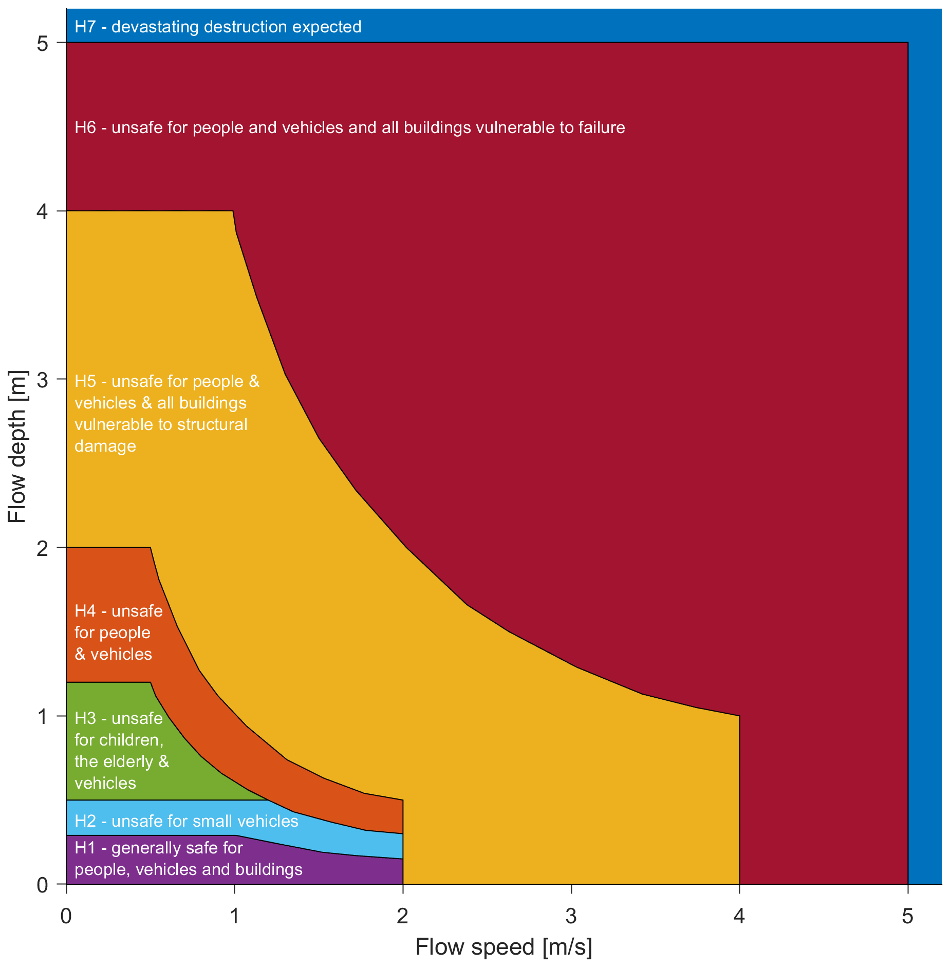
Figure 3 A flood hazard classification scheme from H1 (safe) to H6 (dangerous) recommended for use in Australia. Flood hazard class H7 is additional to the recommended classifications.

2.6 Bernoulli's trial to assess flood hazard class changes

The assessment of climate changes on flood hazard classification had to deal with a range of climate model projections spanning dry through to wet, which have significantly different flood projections and associated flood hazards. Consequently, each flood hazard classification was treated separately, and assessments were done on an annual basis for a historical epoch of 1980 to 1999, and projected epochs of 2020–2039 for near-term, 2050–2069 for medium-term and 2080–2099 for long-term comparisons. These future epochs correspond to those typically used for near, mid and far future horizons in government planning. The occurrences of each flood hazard classification are then the number of times it occurs divided by 20, the number of years within these epochs, which is a maximum likelihood estimate of the occurrence probability given 20 independent binomial (Bernoulli's) trials. Once the occurrence probabilities are known for each epoch in each flood projection, they are averaged or ensembled across the flood projections from the six climate model combinations before estimating changes between epochs.

3 Results

3.1 Calibration of the hydrologic model

The hydrologic model calibration to annual maximum discharge at Gravesend (Fig. 4) was achieved using the same m (nominally stream shape, which is expected) and different k_c (channel storages) and the same small catchment storage parameters (f=0.0005, h_max=0.2 m and u=80 mm d⁻¹) across the six historical climate projections available in NARCliM 1.5. Uncertainty remains with the adopted calibration, which is minimized for inundation hazard assessment by focusing calibration on rarer events.

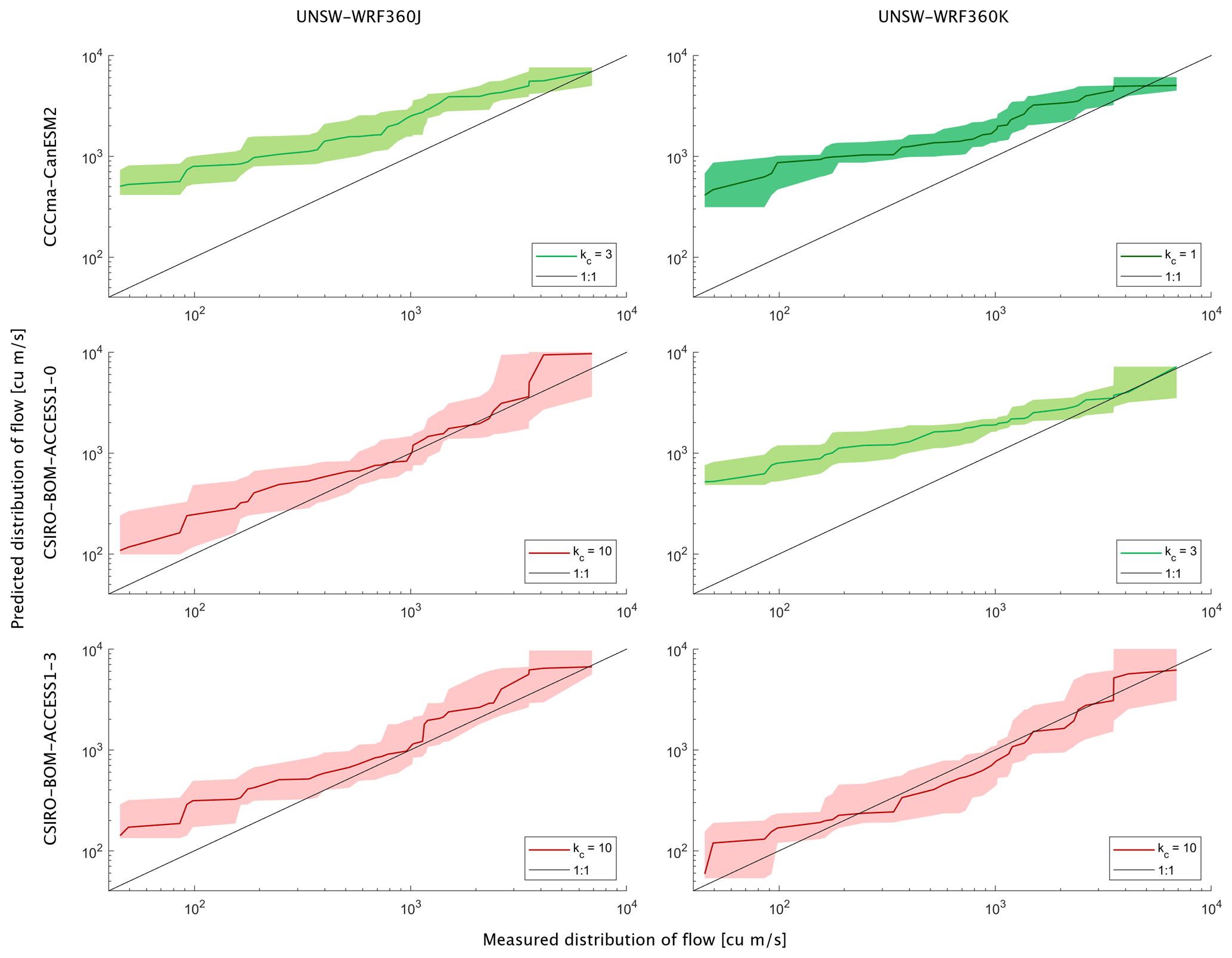
Figure 4 Comparisons between modelled discharge at Gravesend (Fig. 2) with measurements for all global (rows) and regional (columns) climate model combinations. Model discharges includes additional evaporation via local storages (f=0.0005, h_max=0.2 m and u=80 mm d⁻¹). Hydrology model parameter m=0.5 for all cases and k_c is indicated in each panel. Black lines indicate perfect agreement, solid coloured lines and corresponding shaded regions are mean and 95 % confidence of measured distribution when resampled to compare with modelled discharges; different colours indicate different k_c.

3.2 Calibration of the hydraulic model

The hydraulic model, LISFLOOD, was calibrated by varying the main channel depths until it matched previous models, MIKE FLOOD, that had been calibrated to historical floods. The hydraulic model with channel depth at 19 % of the maximum channel depth had mean flood level differences of less than 1 mm (Fig. 5, top left panel) while also being near the lowest standard deviation of flood level difference. As the LISFLOOD and MIKE FLOOD models had different resolutions and consequently different ground surface elevations, comparing depths bring in two changes, one related to hydraulic performance and another related to ground surface elevation interpolation differences (Fig. 5, bottom left panel). Alternatively, comparing water surface levels (Fig. 5, top right panel) removes this ground surface elevation interpolation aspect; however, for models with large vertical variation (e.g. Gwydir River has 100 m vertical change over its 167 km length), this vertical variation overpowers water level differences when plotted. Nevertheless, comparing differences in both depth and water surface level together with an overall water-level difference map (Fig. 5, bottom right panel), provides a visual assessment of model calibration.

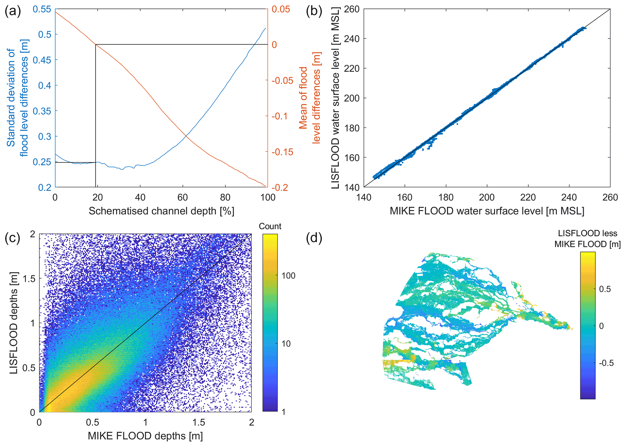
Figure 5 Gwydir River hydraulic model (LISFLOOD) calibration to existing MIKE FLOOD hydraulic models by NSW Environment & Heritage. (a) Selection of schematized channel depth (zero means no channels and 100 % means largest main channels possible from survey) with the black lines showing selected channel depth. (b) A comparison between flood levels across the entire model (blue dots) with perfect fit (black line). (c) A comparison between flood depth across the entire model. (d) Difference map between models.

3.3 Flood hazard classification and changes under RCP 4.5 and RCP 8.5

The occurrence probabilities under both RCP 4.5 and 8.5 (Fig. 6, Table S1) for flood-hazard classification H1 (generally safe for people, vehicles and buildings) are predicted to increase whereas higher hazard classifications (generally dangerous for people, vehicles and buildings) are predicted to decrease in the long term (comparing 2080–2099 with 1980–1999) for the NARCliM 1.5 ensemble. Within this ensemble, the H1 occurrence probability changes for RCP 4.5 vary from no change to an increase of 0.3 and for the RCP 8.5 increases from 0.06 to 0.39 (Figs. S1–S6), indicating a high likelihood of a reduction in flood hazard at the valley scale. This longer-term assessment outcome does not apply to the near or medium term (2020–2039 or 2050–2069, Table S1). The change expected in the near term is very slight (increase in H1 by 0.01 to 0.02) but the ensemble includes projections where the H1 occurrence probability is reduced by 0.09. These decreases in H1 come with increases in H2 through to H4 of between 0.03 to 0.13. The medium-term comparison period is a transition between the other two, with RCP 8.5 always increasing H1 and decreasing H2 through to H4 and RCP 4.5 having both increases and decreases in H1 through to H4 within the ensemble.

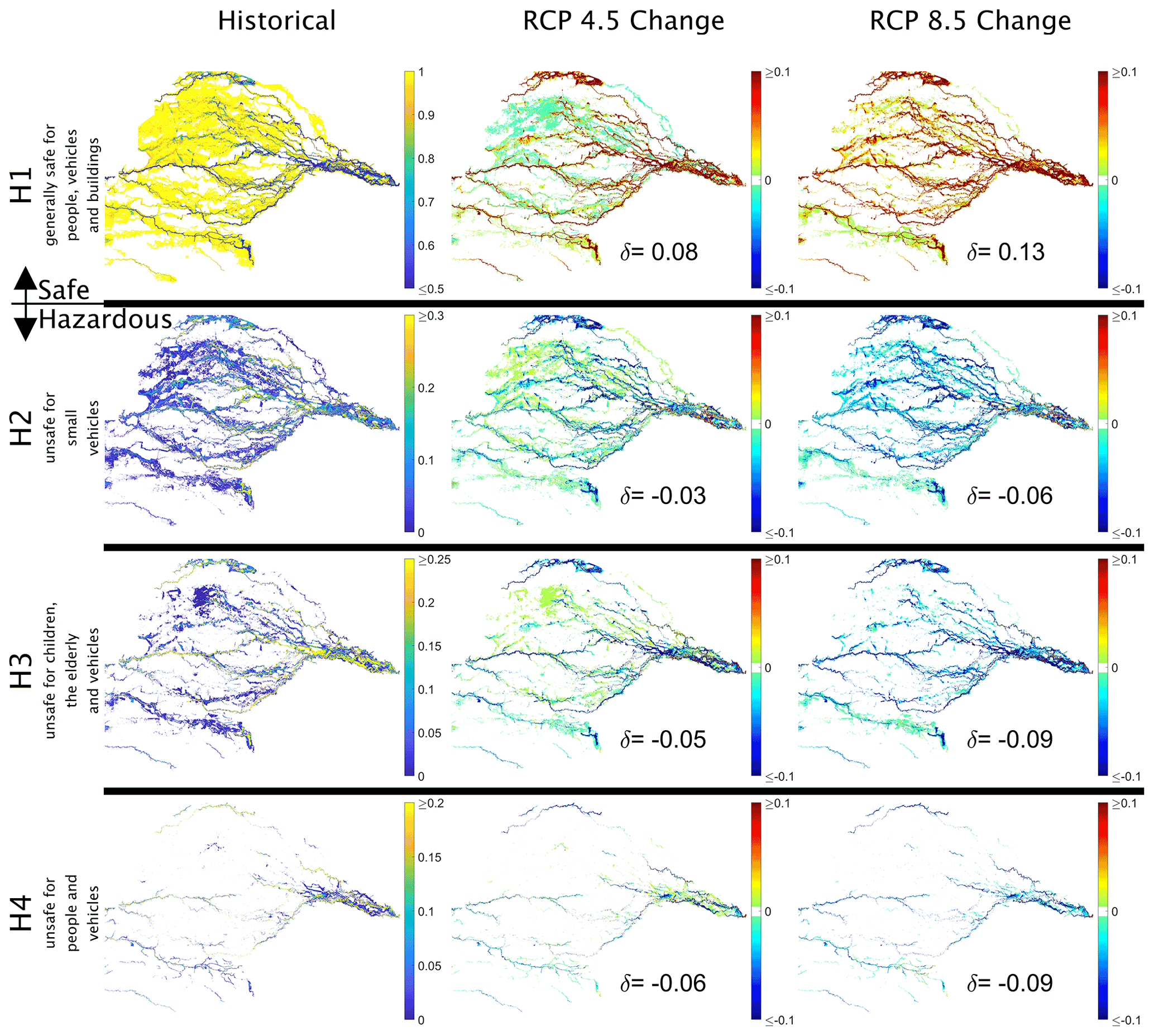
Figure 6 Gwydir Valley flood hazard historical (1980–1999) classification occurrences and their changes under RCP 4.5 and RCP 8.5 (2080–2099) for the NARCliM 1.5 ensemble. The mean of occurrence probability changes, δ, shown in each panel. For brevity, flood hazard historical classifications H5 to H7 are not shown as they are limited to within river and creek channels.

4 Discussion

The increases in H1 occurrence coupled with decreases in H2–H4 (Fig. 6, Table S1 and Figs. S1–S6) indicates that flood hazard is decreasing in the long term under projected climate changes (all cases in the ensemble and both RCP 4.5 and 8.5) in the region modelled (Fig. 2). The near-term changes are more uncertain as there are cases in the ensemble that both increase and decrease flood hazard (Table S1). Comparing the near, medium and long-term, RCP 8.5 shows a more certain decrease in flood hazard compared with RCP 4.5; however, in both scenarios, the most likely outcome is a decrease in flood hazard, with all members of the ensemble forecasting this.

The inference that flood hazard is decreasing in this region with projected climate change comes with several key limitations. Hydrology models were calibrated to best represent infrequent events across the historical period. Consequently, these models overestimate the catchment runoff from frequent events by different amounts for each member of the ensemble (Fig. 4). These differences come from the climate models themselves, where the rainfall runoff is estimated using different approaches, leading to different outcomes across the one historical period. That is, the distribution of runoff of each member of the ensemble for the historical period, in the absence of epistemic uncertainty, should be similar. Although these distributions are different and consequently, add to the uncertainty of inundation depth and speed projections, both are used to assess flood hazards. The hydraulic model, which was constrained reasonably given the differences between resolution and modelling approaches (Fig. 5), is less of an issue than hydrologic uncertainty. However, there are still differences between estimates (Fig. 5) from various flood projections that may lead to different conclusions spatially. Finally, when estimating changes in flood hazard, this would usually involve estimates of flood hazard under extreme conditions. However, the assessment provided used an alternative method for reasons discussed in the following paragraphs.

Conventional extreme value analysis for flood hazard assessments involves establishing a link between flow discharges and exceedance probabilities. This relationship can then be used to assign exceedance probabilities either to historical events or synthetic events that represent historical events, which are simulated, and the spatially varied maximum flood hazard obtained. This approach would work for systems that are driven by one major inflow and have flooded areas that are relatively small compared with the rainfall systems that excite flooding. However, the floodplain being assessed has a large catchment area compared with the spatial size of rainfall events and although it has one major inflow, there are several others, and those combined with the floodplain itself, make breaking continuous simulations into a series of events where the probability is constant across the floodplain-inundated area a subjective (or arbitrary) assessment.

Another issue in using conventional extreme value analysis for flood hazard assessments is the balance between the projection period and the ability to establish reasonable extreme value estimates. For example, one can do a simple numerical experiment in which the two distributions are constructed with a fixed increase in all extremes (simplest case), and then draw one sample; the estimated extreme values, obtained from fitting to this sample, can be both an increase and a decrease compared with that assumed and this is due to sampling error when the analysis period is shorter than the extreme value return period being estimated. To robustly estimate an extreme value, using a one-off sample, the analysis period usually needs to be many times its return period (rule-of-thumb, 10 or more). Without this, the sampling error overwhelms any changes and thus any changes that are within the confidence limits are statistically insignificant.

The final issue in using conventional extreme value analysis comes from the differences in inundation extents and frequency across the climate model projections that span dry through to wet conditions. This led to significant areas that were inundated in the wettest projections that remained dry in the driest projection. Consequently, the members within the ensemble would vary spatially, making uncertainties difficult to understand and communicate.

Applying extreme value theory to individual grid inundation flood hazard (i.e. linking exceedance probability directly to flood hazard, after applying either block maxima or the peak-over-threshold approach to independent and identical distributed events to determine extreme events), as opposed to the conventional method of linking probabilities through event peak discharge, means that the number of extreme events changes from many events along deep watercourses to approaching zero near the edge of maximum inundation. This variation in the number of extreme events led to reasonably consistent spatial projections along deep watercourses to inconsistent spatial projections across the floodplain where the number of extreme events approaches zero at the edge of inundation. These spatially inconsistent projections were obtained for a range of extreme-value approaches and fitting methods. Furthermore, near the edge of maximum inundation, the extreme value models themselves broke down as the number of events approached zero, the net result being very limited consistency in linking exceedance probabilities to flood hazard across the floodplains, particularly near the edge of maximum inundation.

Our approach (Sect. 2.5 and 2.6), where we estimate changes in the annual probability of the occurrence of flood hazard classes overcomes issues with conventional and grid-based extreme value analysis.

5 Summary

A modelling framework for estimating projected flood hazards from regional climate model projections has been presented, including a different approach to assessing flood hazard changes. The modelling framework was applied to Gwydir River (Australia) using New South Wales and Australian Capital Territory Regional Climate Modelling version 1.5 projections with computationally efficient hydrologic and hydraulic models. This included six historical and 12 future regional climate projections occupying the plausible future climate space with similar temperature and drier conditions. This included 6 historical and 12 future regional climate projections occupying the plausible future climate space with warmer temperature and drier conditions than in the history. The simulations were continuous and totalled 1470 years, requiring high-performance computing resources for timely completion. The climate projections included spatially varied rainfall runoff, allowing the implementation of a hydrological modelling approach that only required flow routing, as soil dynamics were included in the regional climate models. The hydrology model was constrained by measured distributions of runoff. The hydraulic modelling approach was selected after an extensive evaluation and testing phase of modelling types with proven track records of computational efficiency, leading to the selection of the partial inertial-wave equation as implemented in LISFLOOD over the other family of efficient approaches under the cellular automata umbrella. This hydraulic model was constrained by modifying the main channel geometry until it matched more detailed and calibrated hydraulic models using the dynamic wave equation. The simulations resulted in spatially varied daily maximum flow depth and flow speeds at those depths across the 18 regional climate projections, allowing flood hazard assessments.

Changes in flooding hazard were assessed by estimating changes in the annual probability of occurrence of a range of flood hazard classes, with the first class, H1, being a safe class and all other classes having various levels of flooding hazard. This approach was taken to overcome several barriers in using conventional flood hazard assessment techniques where flooding hazards are estimated at various extreme values. These barriers included a variable number of hazard events across the floodplain, the ability to determine an extreme value where the underlying processes are changing, through to regional climate projections ranging from dry to wet, leading to significant differences in inundation extents. Changes in annual probability of occurrence in the long term are consistent, across the ensemble for both RCP 4.5 and 8.5, indicating a reduction of flooding hazard across Gwydir River region modelled for the climate futures evaluated. This was demonstrated as an increased probability of occurrence of the safe class (H1) and decreased probability in all the unsafe classes. The outcomes are more mixed in the near term, with the ensemble indicating minor decreases in flooding hazard albeit with ensemble members having both increases and decreases. The medium-term projections are transitional between the near and long term; however, there remain ensemble members with an increased flooding hazard.