About the return period of a catastrophe

When a natural hazard event like an earthquake affects a region and generates a natural catastrophe (NatCat), the following questions arise: how often does such an event occur? What is its return period (RP)? We derive the combined return period (CRP) from a concept of extreme value statistics and theory – the pseudo-polar coordinates. A CRP is the (weighted) average of the local RP of local event intensities. Since CRP's reciprocal is its expected exceedance frequency, the concept is testable. As we show, the CRP is related to the spatial characteristics of the NatCat-generating hazard event and the spatial dependence of corresponding local block maxima (e.g., annual wind speed maximum). For this purpose, we extend a previous construction for max-stable random fields from extreme value theory and consider the recent concept of area function from NatCat research. Based on the CRP, we also develop a new method to estimate the NatCat risk of a region via stochastic scaling of historical fields of local event intensities (represented by records of measuring stations) and averaging the computed event loss for defined CRP or the computed CRP (or its reciprocal) for defined event loss. Our application example is winter storms (extratropical cyclones) over Germany. We analyze wind station data and estimate local hazard, CRP of historical events, and the risk curve of insured event losses. The most destructive storm of our observation period of 20 years is Kyrill in 2002, with CRP of 16.97±1.75. The CRPs could be successfully tested statistically. We also state that our risk estimate is higher for the max-stable case than for the non-max-stable case. Max-stable means that the dependence measure (e.g., Kendall's τ) for annual wind speed maxima of two wind stations has the same value as for maxima of larger block size, such as 10 or 100 years since the copula (the dependence structure) remains the same. However, the spatial dependence decreases with increasing block size; a new statistical indicator confirms this. Such control of the spatial characteristics and dependence is not realized by the previous risk models in science and industry. We compare our risk estimates to these.

1 Introduction

After a natural hazard event such as a large windstorm or an earthquake has occurred in a defined region (e.g., in a country) and results in a natural catastrophe (NatCat), the following questions arise: how often does such a random event occur? What is the corresponding return period (RP, also called recurrence interval)? Before discussing this issue, we underline that the extension of river flood events or windstorms in time and space depends on the scientific and socioeconomic event definition. This definition may vary by peril and is not our topic even though they influence our research object – the RP of a hazard and NatCat event.

The RP of an event magnitude or index is frequently used as a stochastic measure of a catastrophe. For example, there are different magnitude scales for earthquakes (Bormann and Saul, 2009). However, their RP may not correspond with the local consequences since the hypocenter position also determines local event intensities and effects. For floods, regional or global magnitude scales are not in use (Guse et al., 2020). For hurricanes, the Saffir–Simpson scale (National Hurricane Centre, 2020) is a magnitude measure; however, the random storm track also influences the extent of destruction. Extratropical cyclones hitting Europe, called winter storms, are measured by a storm severity index (SSI; Roberts et al., 2014) or extreme wind index (EWI; Della-Marta et al., 2009). Their different definitions result in quite different RPs for the same events. In the rare scientific publications about risk modeling for the insurance industry, such as by Mitchell-Wallace et al. (2017), better and universal approaches for the RP are not offered. In sum, previous approaches are not satisfactory regarding the stochastic quantification of a hazard or NatCat event. This is our motivation to develop a new approach. Building on results of extreme value theory and statistics, we mathematically derive the concept of combined return period (CRP), which is the average of RPs of local event intensities. As we will show by a combination of existing and new approaches from stochastic and NatCat research, the concept of CRP is strongly related to the spatial association/dependence between the local event intensities, their RPs, and corresponding block maxima, such as annual maxima.

Spatial dependence is not suitably considered in previous research about NatCat. The issue is only a marginal topic in the book by Mitchell-Wallace et al. (2017, Sect. 5.4.2.5) about NatCat modeling for the insurance industry. Jongman et al.'s (2014) model for European flood risk considers such dependence explicitly. However, their assumptions and estimates are not appropriate according to Raschke (2015b). In statistical journals, max-stable dependence models have been applied to natural hazards without a systematic test of the stability assumption. Examples are the snow depth model by Blanchet and Davison (2011) for Switzerland and the river flood model by Asadi et al. (2015) for the Upper Danube River system. Max-stable dependence means that the copula (the dependence structure of a bi- or multivariate distribution) and corresponding value of dependence measures are the same for annual maxima as for 10-year maxima or those of a century (Dey et al., 2016). Also, Raschke et al. (2011) proposed a winter storm risk model for a power transmission grid in Switzerland without validation of the stability assumption. The sophisticated model for spatial dependence between local river floods by Keef et al. (2009) is very flexible. However, it needs a high number of parameters, and the spatial dependence cannot be simply interpolated as is possible with covariance and correlation functions (Schabenberger and Gotway, 2005, Sect. 2.4). Besides, the random occurrence of a hazard event is more like a point event of a Poisson process than the draw/realization of a random variable. For instance, the draw of the annual random variable is certain; the occurrence of a Poisson point event in this year is not certain but random.

In the research of spatial dependence by Bonazzi et al. (2012) and Dawkins and Stephenson (2018), the local extremes of European winter storms are sampled by a pre-defined list of significant events. Such sampling is not foreseen in (multivariate) extreme value statistics; block maxima and (declustered) peaks over thresholds (POT) are the established sampling methods (Coles, 2001, Sects. 3.4 and 4.4; Beirlant et al., 2004, Sect. 9.3 and 9.4). Event-wise spatial sampling is a critical task; the variable time lag between the occurrences at different measuring stations, such as river gauging stations, makes it confusing. The corresponding assignment of Jongman et al. (2014) of one local/regional flood peak to peaks at other sites is not convincing, according to the comments by Raschke (2015b). The sampling of multivariate block maxima is simpler. However, the univariate sampling and analysis are also not trivial. An example is the trend over decades in the time series of a wind station in Potsdam (Germany). Wichura (2009) assumes a changed local roughness condition over the time as the reason; Mudelsee (2020) cites climate change as the reason.

The research of spatial dependence of natural hazards is not an end in itself; the final goal is an answer to the question about the NatCat risk. What is the RP of events with aggregate damage or losses in a region equal to or higher than a defined level? By using CRP, we quantify the risk via stochastic scaling of fields of local intensities of historical events and averaging corresponding risk measures. This new approach significantly extends the methods to calculate a NatCat risk curve. Previous opportunities and approaches for a risk estimate are the conventional statistical models that are fitted to observed or re-analyzed aggregated losses (also called as-if losses) of historical events, as used by Donat et al. (2011) and Pfeifer (2001) for annual sums. The advantages of such simple models are the controlled stochastic assumptions and the small number of parameters; the disadvantages are high uncertainty for widely extrapolated values and limited possibilities to consider further knowledge. The NatCat models in the (re-)insurance industry combine different components/sub-models for hazard, exposure (building stock or insured portfolio), and corresponding vulnerability (Mitchell-Wallace et al., 2017, Sect. 1.8; Raschke, 2018); additionally, they offer better opportunities for knowledge transfer such as the differentiated projection of a market model on a single insurer. However, the corresponding standard error of the risk estimates is frequently not quantified (and cannot be quantified). The numerical burden of such complex models is high. Tens of thousands of NatCat events must be simulated (Mitchell-Wallace eta al., 2017, Sect. 1). Thus, the question arises of what the stochastic criterion for the simulation of a reasonable event set in NatCat modeling is. As far as we know, scientific NatCat models for European winter storms (extratropical cyclones) are based on numerical simulations (Della-Marta et al., 2010; Osinski et al., 2016; Schwierz et al., 2010) and are not intensively validated regarding spatial dependence.

To answer our questions, we start with topics of extreme value statistics in Sect. 2, where we recall the concept of max-stability for single random variables, bivariate dependence structures (copulas), and random fields. We also extend Schlather's (2002) first theorem with a focus on spatial dependence. The more recent approaches to area functions (Raschke, 2013) and survival functions (Jung and Schindler, 2019) of local event intensities within a region are implemented therein. In Sect. 3, we derive the CRP from the concept of pseudo-polar coordinates of extreme value statistics and explain its testability, possibility of scaling, and corresponding risk estimate. Subsequently, in Sect. 4, we apply the new approaches to winter storms (extratropical cyclones) over Germany to demonstrate their potential. This application implies several elements of conventional statistics, which are explained in Sect. 5. Finally, we summarize and discuss our results and provide an outlook in Sect. 6. Some stochastic and statistical details are presented in the Supplement and Supplement data. In the entire paper, we must consider several stochastic relations. Therefore, the same mathematical symbol can have different meanings in different subsections. We also expect that the reader is familiar with statistical and stochastic concepts such as statistical significance, goodness-of-fit tests, random fields, and Poisson (point) processes (Upton and Cook, 2008).

2 Max-stability in statistics and stochastic

2.1 The univariate case

Before introducing CRP and its properties, we discuss and extend the concept of max-stability in extreme value statistics, with a focus on random processes and fields. Max-stability has its origin in univariate statistics. The cumulative distribution functions (CDFs) F_n(x) of maximum X_n=Max(X₁ … X_n) of n independent and identically distributed (iid) random variables X_i with CDF F(x) (for the non-exceedance probability Pr(X≤x)) is

$$\begin{array}{}\text{(1)}& F_n\left(x\right)=F(x{)}^n.\end{array}$$

A CDF F(x) is max-stable if the linear transformed maximum (with parameters a_n and b_n) has the same distribution (Coles, 2001, Def. 3.1):

$$\begin{array}{}\text{(2)}& F_n\left(a_{n}x+b_n\right)=F{\left(a_{n}x+b_n\right)}^n=F\left(x\right).\end{array}$$

The Fréchet distribution (Beirlant et al., 2004, Table 2.1) is such a max-stable distribution, also called extreme value distribution, with the following CDF:

$$\begin{array}{}\text{(3)}& G\left(x\right)=\exp \left(-{\displaystyle \frac{\mathrm{1}}{x^{\mathit{\alpha }}}}\right),x\ge \mathrm{0},\mathit{\alpha }>\mathrm{0}.\end{array}$$

For the unit Fréchet distribution, the parameter is α=1, and the transformation parameters are b_n=0 and a_n=n. Most distribution types are not max-stable, but their distribution of maxima (1) converges to an extreme value distribution by increasing sample size n, called the block size in this context (Beirlant et al., 2004, Sect. 3). We can only refer to some of a very high number of corresponding publications (e.g., De Haan and Ferrira, 2007; Falk et al., 2011). Coles (2001) gives a good overview for practitioners.

2.2 Max-stable copulas

It is also well-known that a bivariate CDF F(xy) can be replaced by a copula C(uv) and the marginal CDFs F_x(x) and F_y(y):

$$\begin{array}{}\text{(4)}& F(x,y)=C\left(F_x\left(x\right),F_y\left(y\right)\right)=\mathrm{Pr}(X\le x,Y\le y).\end{array}$$

The copula approach represents a basic distinction between the marginal distributions and the dependence structure; it was introduced by Sklar (1959). As there are different univariate distributions (types), there are different copulas (types). Mari and Kotz (2001) present a good overview about copulas, their construction principles, and different views on dependence. Max-stability is also a property of some copulas, called max-stable copula or extreme copula. A max-stable copula remains the same for pairs of componentwise maxima (X_nY_n) as it was already for the underlying pairs (XY); the copula parameters including dependence measure such as Kendall's (1938) rank correlation are equal. The formal definition is (Dey et al., 2016, Sect. 2.3)

$$\begin{array}{}\text{(5)}& C_n(u,v)=C{\left(u^{\mathrm{1}/n},v^{\mathrm{1}/n}\right)}^n.\end{array}$$

2.3 Max-stability of stochastic processes

The spatial extension of the bivariate situation and corresponding distribution is the random field Z(x) at points x in the space ℝ^d with d dimensions (e.g., Schlather, 2002). In our application, ℝ² is the geographical space, and x is the corresponding coordinate vector. At one point/site, x in ℝ^d, F_x(z) is the marginal distribution of the local random variable Z. There are various differentiations and variants such as (non-)stationarity or (non-)homogeneity. A max-stable random field has max-stable marginal distributions and the copulas between two margins are also max-stable. Schlather (2002) has formulated and proofed a construction of a max-stable random field (we cite his first theorem with nearly the same notation).

Theorem 1: Let Y be a measurable random function and $\mathit{\mu }=\mathbb{E}\underset{{\mathbb{R}}^{\mathrm{d}}}{\int }\max \mathit{\{}\mathrm{0},Y(\mathit{x}\left)\mathit{\right\}}\mathrm{d}\mathit{x}\in (\mathrm{0},\mathrm{\infty })$ . Let Π be a Poisson process on ${\mathbb{R}}^{\mathrm{d}}\times (\mathrm{0},\mathrm{\infty })$ with intensity measure $d\mathrm{\Lambda }(\mathit{y},s)={\mathit{\mu }}^{-\mathrm{1}}\mathrm{d}\mathit{y}{s}^{-\mathrm{2}}\mathrm{d}s$ , and Y_y,s i.i.d. copies of Y; then

$$\begin{array}{}\text{(6)}& \begin{array}{rl}Z\left(\mathit{x}\right)& =\begin{array}{c}\sup \\ (y,s)\in \mathrm{\Pi }\end{array}s{Y}_{\mathrm{y},\mathrm{s}}(\mathit{x}-\mathit{y})\\ & =\begin{array}{c}\sup \\ (y,s)\in \mathrm{\Pi }\end{array}s\max \left\{Y_{\mathrm{y},\mathrm{s}}(\mathit{x}-\mathit{y}),\mathrm{0}\right\}\end{array}\end{array}$$

is a stationary max-stable process with unit Fréchet margins.

Extreme value statistics is interested in the max-stable dependence structure (copula) between the margins, the unit Fréchet distributed random variables Z at fixed points x in space ℝ^d. From the perspective of NatCat modeling in the geographical space ℝ² and with Y(x)≥0, the entire generating process is interesting. The Poisson (point) process Π represents all hazard events (e.g., storms) of a unit period such as a hazard season or a year; it has two parts, s and y. The point events s on (0, ∞) are a stochastic event magnitude and scale the field of local event intensity s_x(x):

$$\begin{array}{}\text{(7)}& s_x\left(\mathit{x}\right)=s{Y}_{\mathrm{y},\mathrm{s}}(\mathit{x}-\mathit{y}),\end{array}$$

which represents all point events s_x(x) at sites x. The random coordinate y is a kind of epicenter in the meaning of NatCat with the (tendentiously) highest local event intensity such as maximum wind speed, maximum hail stone diameter, or peaks of earthquake ground accelerations. The copied random function Y(x) determines the pattern of a single random event in the space ℝ^d. Y(x) or its local expectation converges to 0 or is 0 if the magnitude $\left|\right|\mathit{x}\left|\right|$ of the coordinate vector converges to infinity due to the measurability condition in Theorem 1. This also applies to NatCat events with limited geographical extend.

Schlather (2002) has demonstrated the flexibility of his construction by presenting realizations of maximum fields for different variants of Y(x). Its measurability condition is fulfilled by classical probability density functions (PDFs, first derivative of the CDF; Coles, 2001, Sect. 2.2) of random variables. For instance, Smith (1990, an unpublished and frequently cited paper) used the PDF of the normal distribution. We present some examples of the random function Y(x) in the Supplement, Sect. 4, to illustrate the universality of the approach. Y(x) can also imply random parameters such as variants of standard deviation of applied PDF, and it can be combined with a random field.

Both s and s_x(x) with fixed x are point events of Poisson processes with intensity s⁻²ds. This is the expected point density and determines the exceedance frequency. The latter is the expected number of point events s_x(x)>z and s>z:

$$\begin{array}{}\text{(8)}& \mathrm{\Lambda }\left(z\right)=\underset{z}{\overset{\mathrm{\infty }}{\int }}{s}^{-\mathrm{2}}\mathrm{d}s=\mathrm{1}/z.\end{array}$$

The entire construction of Theorem 1 is also a kind of shot noise field according to the definitions of Dombry (2012). Furthermore, Schlather (2002) has also published a construction of a max-stable random field without a random function but with a stationary random field. The logarithmic variant of Theorem 1 (logarithm of Eqs. 6 and 7) also results in a max-stable random field; however, the marginal maxima are unit Gumbel distributed, and Eq. (8) would be an exponential function. The Brown–Resnick process – well-known in extreme value statistics (e.g., Engelke et al., 2011) – generates a max-stable random field with such unit Gumbel distributions as a result of random walk processes (Pearson, 1905). It is implicitly a construction according to Theorem 1, as for exponential transformation (inverse of logarithmic transformation), and the random walk with drift is the random function of Theorem 1. The origin of a Brown–Resnick process in ℝ^d can be fixed but can also be a random coordinate as y is in Theorem 1.

The construction of Theorem 1 is already used to model natural hazards in the geographical space. Smith (1990) has applied the bivariate normal distribution as Y(x) in a rainstorm modeling. The Brown–Resnick process has already been applied to river flood (Asadi et al., 2015). Blanchet and Davison's (2011) model for snow depth and Raschke et al.'s (2011) model for winter storms, both in Switzerland, are also max-stable. There are also similarities to conventional hazard models. Punge et al.'s (2014) hail simulation includes maximum hail stone diameter that acts like ln (s) in Eqs. (6) and (7). Raschke (2013) already stated similarity between earthquake ground motion models and Schlather's construction. However, the earthquake magnitude can have a wider influence on the geographical event pattern than simple scaling. This was one of our motivations to extend and generalize the Schlather's construction (Eq. 7) with dimension d of R^d:

$$\begin{array}{}\text{(9)}& s_x\left(\mathit{x}\right)=s^{\mathrm{1}+\mathit{\beta }}{Y}_{\mathrm{y},\mathrm{s}}\left({\left((\mathrm{1}+\mathit{\beta })s^{-\mathit{\beta }}\right)}^{-\frac{\mathrm{1}}{d}}(\mathit{x}-\mathit{y})\right),\mathit{\beta }>-\mathrm{1},\end{array}$$

and for the corresponding field of maxima (Eq. 6), we write

$$\begin{array}{}\text{(10)}& \begin{array}{rl}Z\left(\mathit{x}\right)=& \begin{array}{c}\sup \\ (y,s)\in \mathrm{\Pi }\end{array}{s}^{\mathrm{1}+\mathit{\beta }}{Y}_{\mathrm{y},\mathrm{s}}\left({\left((\mathrm{1}+\mathit{\beta })s^{-\mathit{\beta }}\right)}^{-\frac{\mathrm{1}}{d}}(\mathit{x}-\mathit{y})\right),\\ & \mathit{\beta }>-\mathrm{1}.\end{array}\end{array}$$

As we show in the Supplement, Sect. 2, the marginal Poisson processes s_x(x) in Eq. (9) have the same exceedance frequency (Eq. 8) as Eq. (7). Correspondingly, Z(x) in Eq. (10) is also unit Fréchet distributed as in Eq. (6). Schlather's construction is a special case of Eqs. (9) and (10) with β=0; Eqs. (9) and (10) only imply max stability of spatial dependence in this case, which is what we discuss in the following section.

2.4 Spatial characteristics and dependence

We now illustrate spatial max-stability and its absence by examples of Eqs. (9) and (10) with standard normal PDF as random function Y(x) in a one-dimensional parameter space ℝ^d=1. For this purpose, we apply the simulation approach of Schlather (2002) and generate random events within a range (−10, 10) for local event intensities within the region/range (−4, 4) in ℝ¹ by a Monte Carlo simulation. According to Schlather's procedure, which processes a series of random numbers from a (pseudo-)random generator, only the events for the large s are simulated; this implies incompleteness for smaller events. This does not significantly affect the simulated field Z(x) of maxima. However, we can only consider this simulation for β≥0 in Eqs. (9) and (10) since the edge effects increase for increasing s if β<0. In Fig. 1a, we show fields for one realization Π of Schlather's theorem (n=1, equivalent to 1 year or one season in NatCat modeling) for the max-stable case with β=0 in Eqs. (9) and (10). With the same series of random numbers, we generate fields of n=100 realizations of Π in Fig. 1b. It has the same pattern n=1 and is the same when we linear transform the local intensities s_x, with division by n=100. The entire generating processes are max-stable, just as the resulting marginals and association/dependence between marginals are. In contrast to this total max-stability, the example with β=0.1 results in different patterns for n=1 and n=100 in Fig. 1c and d. The shape of the event fields gets sharper for larger s; only the marginals are max-stable, not their spatial relations.

Figure 1 Examples of simulated fields of local event intensities and enveloping field of maxima (bold green line) generated with standard normal PDF as Y(x) in (6, 7, 9, 10) and the same series of numbers from pseudo-random generator: (a) max-stable and n=1, (b) max-stable and n=100, (c) non-max-stable and n=1, and (d) non-max-stable and n=100. The strongest event has a broken red line.

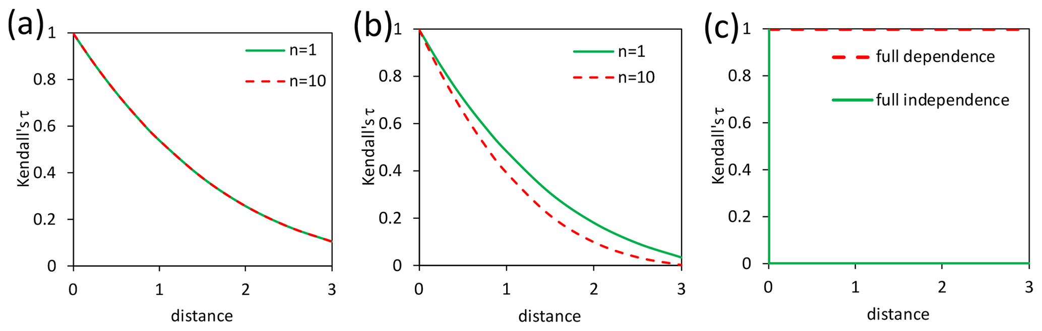
Figure 2 Spatial dependence in relation to the distance measured by Kendall's τ: (a) max-stable fields of Fig. 1, (b) non-max-stable fields of Fig. 1, and (c) limit cases.

To illustrate the effect on spatial dependence quantitatively, we have generated local maxima Z(x) from Eq. (10) by Monte Carlo simulation with 100 000 repetitions and the computed corresponding dependence measure Kendall's τ (Kendall, 1938; Mari and Kotz, 2001, Sect. 6.2.6). As depicted in Fig. 2a and b, the functions are the same if β=0 and differ if β=0.1; the dependence is decreasing by increasing n if β>0. In Fig. 2c, the functions are shown for the limit cases of full dependence with the same value of s_x(x) at each point x and full independence with s_x(x)=0 everywhere except one point.

Beside our extension of Schlather's theorem, we also consider a more recent approach from NatCat research to understand the spatial characteristics. Raschke (2013) described an earthquake event by its area function for the peak ground accelerations. This is a cumulative function and measures the set of points in the geographical space (the area) with an event intensity higher than the argument of the function. The area function is limited here to a region and is normalized as follows (u and l symbolizes the region's bounds, the integral in the denominator is the area of the region in ℝ², I_A is an indicator function):

$$\begin{array}{}\text{(11)}& A\left(z\right)={\displaystyle \frac{\underset{l}{\overset{u}{\int }}{I}_A\left(s_x\left(x\right)>z\right)\mathrm{d}x}{\underset{l}{\overset{u}{\int }}\mathrm{d}x}}.\end{array}$$

It is now like a survival function of a random variable (decreasing with the value of functions between 0 and 1), which describes the exceedance probability in contrast to a CDF for non-exceedance probability (Upton and Cook, 2008). Jung and Schindler (2019) have already applied such aggregating functions to German winter storm events and call them explicitly a survival function. However, not every normalized aggregating decreasing function is based on an actual random variable. Moreover, survival functions are not used in statistics to describe regions of random fields or random function as far as we know. Nonetheless, we use the area function (Eq. 11) to characterize and research the spatiality of the event field s_x(x) in a defined region. As an example, the area function for the strongest events in Fig. 1 is shown in Fig. 3a. The differences between the variants n=1 versus n=100 and β=0 versus β=0.1 correspond with the differences between these events in Fig. 1. In Fig. 3b, the limit cases are depicted to illustrate the underlying link between area function and spatial dependence.

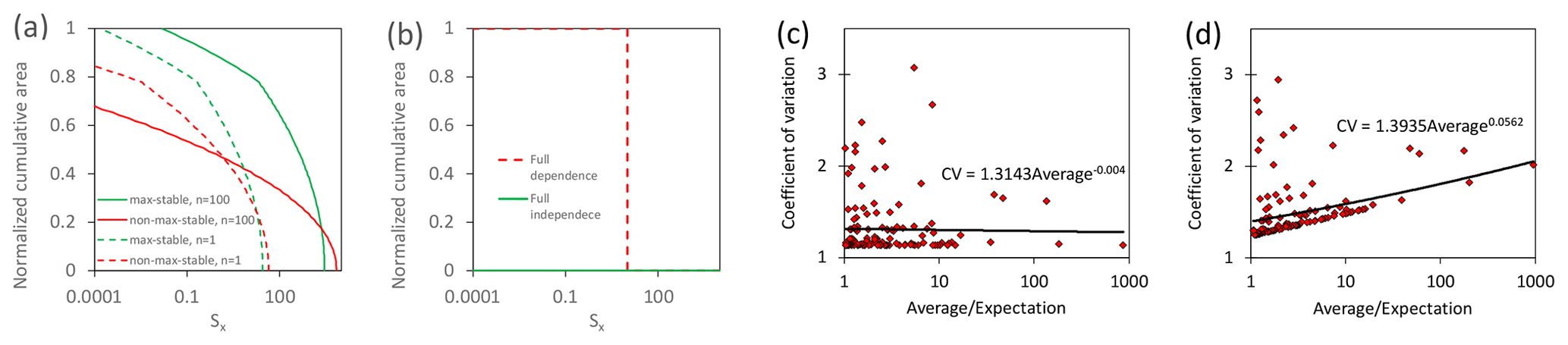
Figure 3 The area function and corresponding characteristics: (a) area function of the biggest event of Fig. 1, (b) area functions for the limit cases (examples), and (c) relation of CV to average for the max-stable case of Fig. 1b and (d) for the non-max-stable case of Fig. 1d (for events with average > 1, the distance between the support points is 0.1 for the computation of the average in the region [−4, 4]).

We also use the parameters of a random variable Z with PDF f(x) and CDF F(z), as well as survival function $\overline{F}\left(z\right)=\mathrm{1}-F\left(z\right)$, to characterize our area function. These parameters are expectation 𝔼[Z] (estimated by sample mean/average), variance Var[Z], standard deviation SD[Z] (the square root of variance), and a coefficient of variation (CV) Cv[Z] (Coles, 2001, Sect. 2.2; Upton and Cook, 2008) with

$$\begin{array}{}\text{(12)}& \begin{array}{rl}& \mathbb{E}\left[Z\right]=\underset{-\mathrm{\infty }}{\overset{\mathrm{\infty }}{\int }}zf\left(z\right)\mathrm{d}z=\underset{I_A}{\overset{\mathrm{0}}{\int }}z\mathrm{d}\overline{F}\left(z\right),\\ & \mathrm{Var}\left[Z\right]=\underset{I_A}{\overset{\mathrm{0}}{\int }}(z-\mathbb{E}[Z\left]{)}^{\mathrm{2}}\mathrm{d}\overline{F}\right(z),\mathrm{SD}[Z]=\sqrt{\mathrm{Var}\left[Z\right]},\\ & \mathrm{CV}={\displaystyle \frac{\mathrm{SD}\left[Z\right]}{\mathbb{E}\left[Z\right]}}.\end{array}\end{array}$$

According to Eq. (12), any scaling of Z by a factor S>0 results in proportional scaling of expectation and standard deviation in Eq. (12), and the CV remains constant. Correspondingly, random magnitude s in Eqs. (9) and (10) only scales the field s_x(x) in the max-stable case with β=0 and influences the expectation of A(z) but not the CV. Thus, the CV is independent from the expectation. This does not apply to the non-max-stable case with β≠0 in Eqs. (9) and (10). These different behaviors are detectable for the examples of Fig. 1b and d in Fig. 3c and d. For the max-stable case, the scale/slope parameter of the linearized regression function does not differ significantly from 0 according to the t test (Fahrmeir et al., 2013, Sect. 3.3). For the max-stable case, the regression function is statistically significant with a p value of 0.00. Linearization is provided by the logarithm of CV and expectation/average. For completeness, the full dependence case of Fig. 3b corresponds with a CV of 0.

As per Sect. 2, Schlather's first theorem has parallels to NatCat models, is used already in hazard models, and was extended here to the non-max-stable case regarding the spatial dependence and characteristics. Statistical indication for max-stability is the independence of the spatial dependence measure from the block size (e.g., 1 versus 10 years) and independence between CV and expectation of the area function (Eq. 11). Otherwise, non-max-stability is indicated.

3 The combined return period (CRP)

3.1 The stochastic derivation

Let the point event Y_x,i be the local intensity at site x of a hazard event and i be a member of the set of all events of a defined unit period such as a year, hazard season, or half season. This local event intensity might be the maximum river discharge of a flood, the peak ground acceleration of an earthquake, or the maximum wind gust of a windstorm event. The entire number of events with $Y_{x,i}>y$ during the unit period is $K={\sum }_{i=\mathrm{1}}^{\mathrm{\infty }}{I}_A(Y_{x,i}>y)$. K is (at least approximately) a Poisson-distributed (Upton and Cook, 2008) discrete random variable with an expectation – the expected exceedance frequency – that is the local hazard function in a NatCat model (this is not the hazard function/hazard rate of statistical survival analysis; Upton and Cook, 2008):

$$\begin{array}{}\text{(13)}& {\mathrm{\Lambda }}_y\left(y\right)=\mathbb{E}\left[K\right].\end{array}$$

This is the bijective frequency function and the local hazard curve. Its reciprocal determines the hazard curve for the RP:

$$\begin{array}{}\text{(14)}& T_y\left(y\right)={\displaystyle \frac{\mathrm{1}}{{\mathrm{\Lambda }}_y\left(y\right)}}={\displaystyle \frac{\mathrm{1}}{\mathbb{E}\left[K\right]}}.\end{array}$$

As Y_x is a point event, its RP T=T_y(Y_x) is also a point event of a point process with frequency function according to Eq. (14) but now with the argument/threshold variable z since the scale unit is changed:

$$\begin{array}{}\text{(15)}& {\mathrm{\Lambda }}_T\left(z\right)=\mathrm{1}/z.\end{array}$$

Since Eq. (15) is the same as Eq. (8), Schlather's theorem and our extensions directly apply to RP with T=s_x in Eqs. (7) and (9). For completeness, the marginal maxima have a CDF for n unit periods (a unit Fréchet distribution for n=1 according to Eq. 3):

$$\begin{array}{}\text{(16)}& G_n\left(z\right)=\exp \left(-n{\mathrm{\Lambda }}_T\left(z\right)\right)=\exp (-n/z).\end{array}$$

This is applicable because the probability of non-exceedance for level z of the block maxima is the same probability as per which no events occur with T>z, which is determined by the Poisson distribution; Eq. (6) also implies this link, and Coles (2001, p. 249 “y_p”) has also mentioned this. The same applies to the relation between frequency and maxima of local event intensity.

Schlather's theorem is also based on and implies the concept of pseudo-polar coordinates. According to De Haan (1984) and explained well by Coles (2001, Sect. 8.3.2), two linked max-stable point processes with expected exceedance frequency (Eq. 15) and point events T₁ and T₂ are also represented by pseudo-polar coordinates with radius R and angle V:

$$\begin{array}{}\text{(17)}& \begin{array}{rl}& \left\{R=T_{\mathrm{1}}+T_{\mathrm{2}},V={\displaystyle \frac{T_{\mathrm{1}}}{T_{\mathrm{1}}+T_{\mathrm{2}}}}\right\}⟺\\ & \left\{T_{\mathrm{1}}=RV,T_{\mathrm{2}}=R(\mathrm{1}-V)=T_{\mathrm{1}}{\displaystyle \frac{\mathrm{1}-V}{V}}\right\}.\end{array}\end{array}$$

As we describe in the Supplement, Sect. 1, the expectation of $(\mathrm{1}-V)/V$ is 1 and for the conditional expectation of unknown RP T₂ with known T₁ applies (association is provided):

$$\begin{array}{}\text{(18)}& \mathbb{E}\left[T_{\mathrm{2}}\left|T_{\mathrm{1}}\right.\right]=T_{\mathrm{1}}.\end{array}$$

The interest in extreme value theory and statistics (Coles, 2001, Sect. 3.8; Beirlant et al., 2004, Sect. 8.2.3; Falk et al., 2011, Sect. 4.2) is focused on the distribution of pseudo-angle V with CDF H(z). As Coles (2001) writes “the angular spread of points of N [the entire point processes] is determined by H, and is independent of radial distance [R]”, angle and radius occur independently from each other, and H determines the copula between two marginal maxima Z(x) in Theorem 1.

According to Coles (2001, Sect. 3.8), the pseudo-radius R in Eq. (17) is a point event of a Poisson process with frequency $\mathrm{\Lambda }\left(z\right)=\mathrm{2}/z$ – the double of Eq. (15). This means the average of two RPs, T₁ and T₂, results in a combined return period (CRP) T_c,

$$\begin{array}{}\text{(19)}& T_{\mathrm{c}}={\displaystyle \frac{T_{\mathrm{1}}+T_{\mathrm{2}}}{\mathrm{2}}},\end{array}$$

with exceedance frequency function (Eqs. 8 and 15). We do not have a mathematical proof that Eqs. (18) and (19) also apply to non-max-stable-associated point processes. However, max-stable and non-max-stable cases have the same limits: full dependence (T₁=T₂) and no dependence/full independence (T₁=0 if T₂>0 and vice versa; T=0 represents the lack of a local event). Therefore, Eq. (19) should also apply to the non-max-stable case between these limits. This can be heuristically validated as we demonstrate by an example in the Supplement, Sect. 3.

More than one RP can be averaged since the averaging of two RPs can be done in serial (and the pseudo-polar coordinates are also applied to more than two marginal processes). Serial averaging (averaging the last result with a further RP) also implies a weighting; the first considered RPs would be less weighted than the last in the final CRP. The general formulation of averaging of RP with weight w is

$$\begin{array}{}\text{(20)}& T_{\mathrm{c}}={\displaystyle \frac{{\sum }_{i=\mathrm{1}}^n{T}_i{w}_i}{{\sum }_{i=\mathrm{1}}^n{w}_i}}.\end{array}$$

The corresponding continuous version within the region's bounds u and l in space ℝ^d is

$$\begin{array}{}\text{(21)}& T_{\mathrm{c}}={\displaystyle \frac{\underset{l}{\overset{u}{\int }}T\left(x\right)w\left(x\right)\mathrm{d}x}{\underset{l}{\overset{u}{\int }}w\left(x\right)\mathrm{d}x}}.\end{array}$$

If w(x)=1 applies in Eq. (21), then the denominator is the area of the region. Furthermore, the CRP T_C is the expectation of the area function (Eq. 11). This also applies to other weightings if we consider it in the area function, here written for RP T(x),

$$\begin{array}{}\text{(22)}& A\left(z\right)={\displaystyle \frac{\underset{l}{\overset{u}{\int }}w\left(x\right)I_A\left(T\right(x)\ge z)\mathrm{d}x}{\underset{l}{\overset{u}{\int }}w\left(x\right)\mathrm{d}x}},\end{array}$$

with empirical version for n measuring stations in the analyzed region:

$$\begin{array}{}\text{(23)}& A\left(z\right)={\displaystyle \frac{{\sum }_{i=\mathrm{1}}^n{w}_i{I}_A\left(T_i\ge z\right)}{{\sum }_{i=\mathrm{1}}^n{w}_i}}.\end{array}$$

The weighting, especially the empirical one, can be used in hazard research to compensate for an inhomogeneous geographical distribution of measurement stations or a different focus than the covered geographical area such as the inhomogeneous distribution of exposed values or facilities in NatCat research. It has the same effect on the area function as a distortion of the geographical space as used by Papalexiou et al. (2021). Weighted or not, CRP and CV are parameters of the area function.

3.2 Testability

Before the CRP is applied in stochastic NatCat modeling, it should be tested statistically to validate the appropriateness. A sample of CRPs can be tested by a comparison of its exceedance frequency function (Eq. 15) and their empirical variant. Therein the empirical exceedance frequency of the largest CRP in the sample is the reciprocal of the length of the observation period. The second largest CRP is hence associated with twice the exceedance frequency of the largest CRP and so on. It is the same as for empirical exceedance frequency for earthquake (e.g., the well-known Gutenberg–Richter relation in seismology; Gutenberg and Richter, 1956). However, not all small events are recorded; the sample is thinned and incomplete. This completeness issue is well known for earthquakes and is less important here if only the distribution (Eq. 16) of maximum CRPs is tested. There are several goodness-of-fit tests (Stephens, 1986, Sect. 4.4) for the case of known distribution. The Kolmogorov–Smirnov test is a popular variant.

3.3 The scaling property of CRP

The CRP also offers the opportunity of stochastic scaling. The CRP T_c and all n local RPs T_i in Eq. (20) (and T(z) in Eq. 21) are scaled by a factor S>0:

$$\begin{array}{}\text{(24)}& T_{\mathrm{cs}}=S{T}_{\mathrm{c}}={\displaystyle \frac{{\sum }_{i=\mathrm{1}}^{n}S{T}_i{w}_i}{{\sum }_{j=\mathrm{1}}^n{w}_i}},T_{\mathrm{s},i}=S{T}_i.\end{array}$$

This means for the pseudo-polar coordinates in Eq. (17), which applies to the max-stable case, that

$$\begin{array}{}\text{(25)}& \begin{array}{rl}{R}_{\mathrm{s}}& =S{T}_{\mathrm{1}}+S{T}_{\mathrm{2}}=SR,\\ & V_{\mathrm{s}}={\displaystyle \frac{T_{\mathrm{s},\mathrm{1}}}{T_{\mathrm{s},\mathrm{1}}+T_{\mathrm{s},\mathrm{2}}}}={\displaystyle \frac{S{T}_{\mathrm{1}}}{S\left(T_{\mathrm{1}}+T_{\mathrm{2}}\right)}}=V.\end{array}\end{array}$$

The pseudo-angle V is not changed as expected since pseudo-radius and pseudo-angle are independent in the pseudo-polar coordinate for the max-stable case (Sect. 3.1). This also means that a scaling must be more complex if there is non-max-stability. We cannot offer a general scaling method for this situation; however, it must consider/reproduce the pattern of the relation CV versus CRP (example in Fig. 3d) adequately. Irrespective of this, the corresponding event field of local intensities (e.g., maximum wind gust speed) can be computed for the scaled local RPs via the inverse of the local hazard function: T(z) in Eq. (14) or Λ(z) in Eq. (13).

3.4 Risk estimates by scaling and averaging

The main goal of a NatCat risk analysis is the estimate of a risk curve (Mitchell-Wallace et al., 2017, Sect. 1), the bijective functional of event loss in a region, and the corresponding RP, which is called the event loss return period (ELRP) T_E. As mentioned, there are two approaches for such estimates with corresponding pros and cons.

We introduce an alternative method. Under the assumption of max-stability between ELRP T_E and CRP T_C, according to Eq. (18) with T₁=T_C and T₂=T_E, the expectation of an unknown ELRP T_E is the CRP T_C of the local event intensities. This means that the CRP is an estimate of ELRP. We can average the CRP of many events with the same event loss to get a good estimate of ELRP. However, observations of events with the same loss are not available. Nonetheless, we can exploit the stochastic scaling property of CRP to rescale the local intensity observations of historical events to get the required information. The modeled event loss L_E is the sum of the product of local loss ratio L_R, determined by local event intensity y_x,i and local exposure value E_i over all sites i (Klawa and Ulbrich, 2003; Della-Marta et al., 2010),

$$\begin{array}{}\text{(26)}& L_{\mathrm{E}}=\sum _{i=\mathrm{1}}^n{L}_{\mathrm{R},i}\left(y_{x,i}\right)E_i,\end{array}$$

with the local vulnerability function $L_{\mathrm{R},i}\left(y_{x,i}\right)$. To get the event loss for the scaled event, the observed y_x,i is replaced by

$$\begin{array}{}\text{(27)}& y_{x\mathrm{s},i}={\mathrm{\Lambda }}_{y,i}^{-\mathrm{1}}\left({\displaystyle \frac{{\mathrm{\Lambda }}_{y,i}\left(y_{x,i}\right)}{S}}\right)=T_{y,i}^{-\mathrm{1}}\left(S{T}_{y,i}\left(y_{x,i}\right)\right),\end{array}$$

with local hazard function (Eqs. 13 and 14) and its inverse function. The scaling factor S in Eq. (27) is the same for all sites/locations i, as it is in Eq. (24) for the CRP. This factor S must be adjusted iteratively until the result of Eq. (26) converges to the desired event loss. The scheme in Fig. 4a includes all elements and relations of the scaling approach. Therein, the numerical determination in the scaling scheme has only one direction, from scaled CRP to the event loss. The idea of CRP averaging is also illustrated by Fig. 4b. The standard error of the averaging is the same as for the estimates of an expectation by the sample mean (Upton and Cook, 2008, keyword central limit theorem).

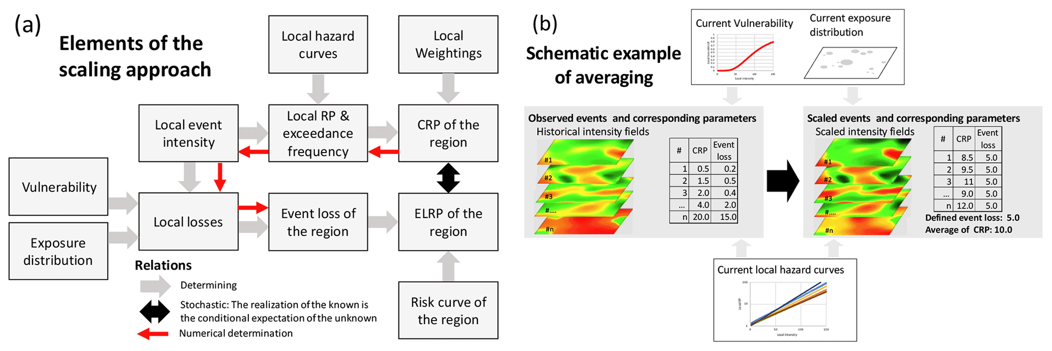
Figure 4 Schemes of the scaling approach: (a) elements and relations, (b) schematic example for estimation of RP of event loss by averaging of CRP.

According to the delta method (Coles, 2001, Sect. 2.6.4), statistical estimates and their standard error can be approximately transferred in another parameter estimation and corresponding standard error by the determined transfer function and its derivatives. A condition of this linear error transfer is a relatively small standard error of the original estimates. The delta method could be used to compute the reciprocal of ELRP – the exceedance frequency and corresponding standard error – or the exceedance frequency is computed directly by averaging the reciprocal of scaled CRPs, and the transfer proxy acts implicitly. We also apply the idea of linear transfer proxy when we average the modeled event loss for the historical events being scaled to the same defined CRP. The unknown sample of ELRPs, which represents the ELRP's distribution for a fixed CRP, is implicitly transferred to a sample of event loss. If the proxies perform well, the difference to the risk estimates via CRP averaging should be small.

There is a further chain of thoughts as argument for the different variants of averaging. The scaling implies subsets of intensity fields of all possible intensity fields. The links between the fields of a subset are determined by the scaling of their CRPs. Correspondingly, every subset generates a risk curve with CRP (now also an ELRP) versus event loss. We also assume a certain unknown probability per subset that is applied if all these subsets generate the entire risk curve via an integral like the expectation of a random variable (Eq. 12). The corresponding empirical variant (estimator) is the averaging. However, we can average three values: CRP, exceedance frequency, or event loss.

All mentioned estimators for risk curve via scaling and averaging over n events are

$$\begin{array}{}\text{(28)}& \begin{array}{rl}& {\widehat{T}}_{\mathrm{E}}\left(L_{\mathrm{E}}\right)={\displaystyle \frac{\mathrm{1}}{n}}\sum _{i=\mathrm{1}}^n{T}_{\mathrm{cs},i}\left(L_{\mathrm{E}}\right),\\ & {\widehat{\mathrm{\Lambda }}}_{\mathrm{E}}\left(L_{\mathrm{E}}\right)={\displaystyle \frac{\mathrm{1}}{n}}\sum _{i=\mathrm{1}}^n\mathrm{1}/T_{\mathrm{cs},i}\left(L_{\mathrm{E}}\right)\\ & {\widehat{L}}_{\mathrm{E}}\left(T_{\mathrm{E}}\right)={\displaystyle \frac{\mathrm{1}}{n}}\sum _{i=\mathrm{1}}^n{L}_{\mathrm{E},i}\left(T_{\mathrm{cs}}=T_{\mathrm{E}}\right).\end{array}\end{array}$$

The right side of the equations in Eq. (28) implies actual values which can be and are being replaced by estimates. Corresponding uncertainties must be considered in the final error quantification.

We draw attention to the fact that the explained scaling does not change the CV of Eq. (23); this implies independence between CRP and CV (Sect. 2.4). Therefore, the presented scaling only applies to the max-stable case of local hazard. For the non-max-stable case, the scaling factor S in Eq. (27) must be replaced event-wise by S_i, which reproduces the observed relation between CRP and CV. An example without max-stability was already shown in Fig. 3d.

4 Application to German winter storms

4.1 Overview about data and analysis

We have selected the peril of winter storms (also called extratropical cyclones or winter windstorms) over Germany to demonstrate the opportunities of the CRP because of good data access and since we are familiar with this peril (Raschke et al., 2011; Raschke, 2015a). Our analysis follows the scheme in Fig. 4a, important results are presented in the subsequent sections, and the technical details are explained in Sect. 5. At first, we provide an overview.

We analyzed 57 winter storms over 20 years from autumn 1999 to spring 2019 (Supplement data, Tables 1 and 2) to validate the CRP approach. Different references (Klawa and Ulbrich, 2003; Gesamtverband Deutscher Versicherer, 2019; Deutsche Rück, 2020) have been considered to select the time window per event. In our definition, the winter storm season is from September to April of the subsequent year. It accepts a certain opportunity of contamination of the sample of block maxima by extremes from convective windstorm events and a certain opportunity of incompleteness from extratropical cyclones outside our season definition. The term winter storm is only based on the high frequency of extratropical cyclones during the winter. The seasonal maximum is also the annual maximum of this peril.

The maxima per half season (bisected by the turn of the year) are analyzed to double the sample size and to increase estimation precision. The appropriateness of this sampling is discussed in Sect. 5.1. We considered records of wind stations in Germany of the German meteorological service (DWD, 2020; FX_MN003, a daily maximum of wind peaks (m s⁻¹), usually wind gust speed) that include minimum record completeness of 90 % for analyzed storms, at least 90 % completeness for the entire observation period, and minimum 55% completeness per half season. Therefore, we only consider 141 of 338 DWD wind stations (Supplement data, Table 3). We think this is a good balance between large sample size and high level of record completeness.

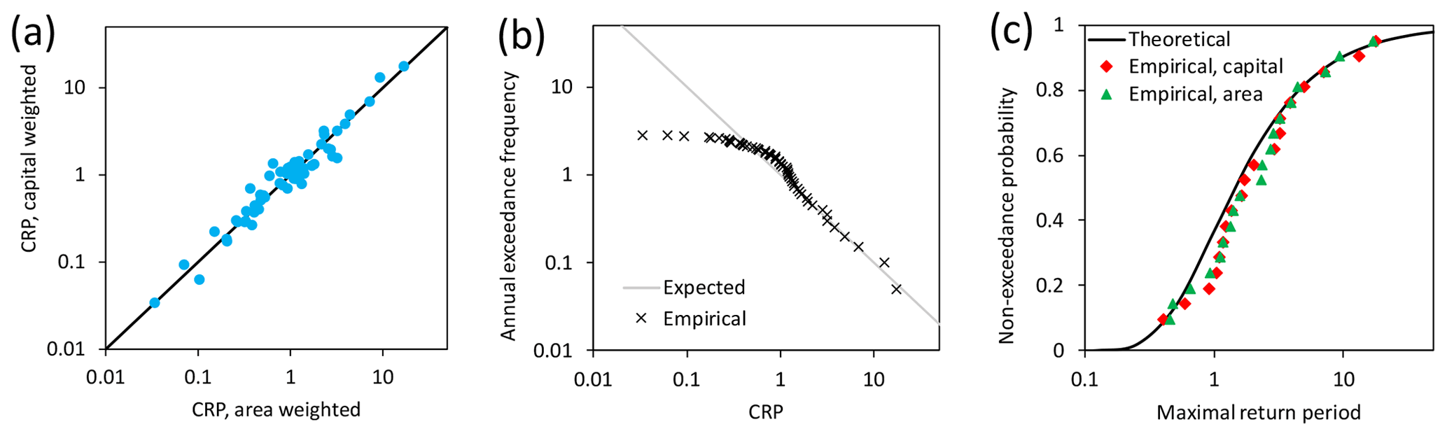
Figure 5 Results of the analysis: (a) comparison of area and capital-weighted CRPs, (b) comparison of theoretical and observed exceedance frequency of capital-weighted CRP, and (c) test of distribution of seasonal maxima of CRP.

The intensity field per event is represented by the maximum wind gust for the corresponding time window of the event at each considered wind station. The local RP per event is computed by a hazard model per wind station. This is an implicit part of the estimated extreme value distribution per station, as explained in Sect. 5.1. The resulting CRPs per event and corresponding statistical tests are presented in the following Sect. 4.2. We have considered two weightings per station, capital, and area. Both are computed per wind station by assigning the grid cells with capital data of the Global Assessment Report (GAR data; UNISDR, 2015) via the smallest distance to a wind station. We also use these capital data to spatially distribute our assumed total insured sum of EUR 15.23 trillion for property exposure (residential building, content, commercial, industrial, agriculture, and business interruption) in Germany in 2018. This is based on Waisman's (2015) assumption for property insurance in Germany and is scaled to exposure year 2018 under consideration of inflation in the building industry (Statistisches Bundsamt, 2020) and increasing building stock according to the German insurance union (GDV; GDV, 2019). It is confirmed by the assumptions of Perils AG (2021); however, their data product is not public. We also used loss data of the GDV (2019) for property insurance when we fitted the vulnerability parameters for the NatCat model. These event loss data of 16 storms during a period of 17 years are already scaled by GDV to exposure year 2018.

The spatial characteristics are analyzed in Sect. 4.3 according to Sect 2.4, focusing on the question of if there is max-stability or not in the spatial dependence and characteristics. Finally, we present the estimated risk curve for the portfolio of the German insurance market in Sect. 4.4 including a comparison with previous estimates. Details of the vulnerability model are documented in Sect. 5.2. The concrete numerical steps, the applied methods to quantify the standard error of estimates, and the consideration of the results from vendor models are explained in Sect. 5.3–5.5, respectively.

4.2 The CRP of past events and validation

As announced, we have computed the CRP according to Eq. (20) with the wind gust peaks listed in the Supplement data, Table 2, and local hazard models according to Eq. (30). Our local hazard models are discussed in Sect. 5.1 and parameters are presented in the Supplement data, Table 4. An example for a complete CRP calculation is also provided therein (Table 8). We have considered two weightings for the CRP, a simple area weighting and a capital weighting (Supplement data, Table 3). In Fig. 5a, we compare the estimates which do not differ so much; the approach is robust in the example. The most significant winter storm of the observation period is Kyrill that occurred in 2007. It has CRPs of 16.97±1.75 and 17.64±1.81 years (area and capital). Both are around the middle of the estimated range of 15 to 20 years (Donat et al., 2011). Further estimates are listed in the Supplement data, Table 1.

In Fig. 5b, the results are validated according to Sect. 3.2. The empirical exceedance frequency matches well with the theoretical one for T_c≥1.65. Small CRPs are affected by the incompleteness of our record list. In the medium range, the differences between the model and empiricism are not statistically significant. In detail, we observe 27 storms with T_c≥1 within 20 years; 20 storms were expected. According to the Poisson distribution, the probability of 27 exceedances or more is 7.8 %. A two-sided test with α=5 % would reject the model if this exceedance probability were 2.5 % or smaller.

The seasonal and annual maxima of CRP must follow a unit Fréchet distribution (α=1 in Eq. 3) according to Eq. (16). We plot this and the empirical distribution in Fig. 5c. The Kolmogorov–Smirnov (KS) test (Stephens, 1986, Sect. 4.4) for the fully specified distribution model does not reject our model at the very high significance level of 25 % for the capital-weighted variant. Usually, only the level of 5 % is considered. This result should not be affected seriously by the absence of one (probably the smallest) maximum due to incompleteness issues. In summary, we state that the CRP offers a stable, testable, and robust method to stochastically quantify winter storms over Germany.

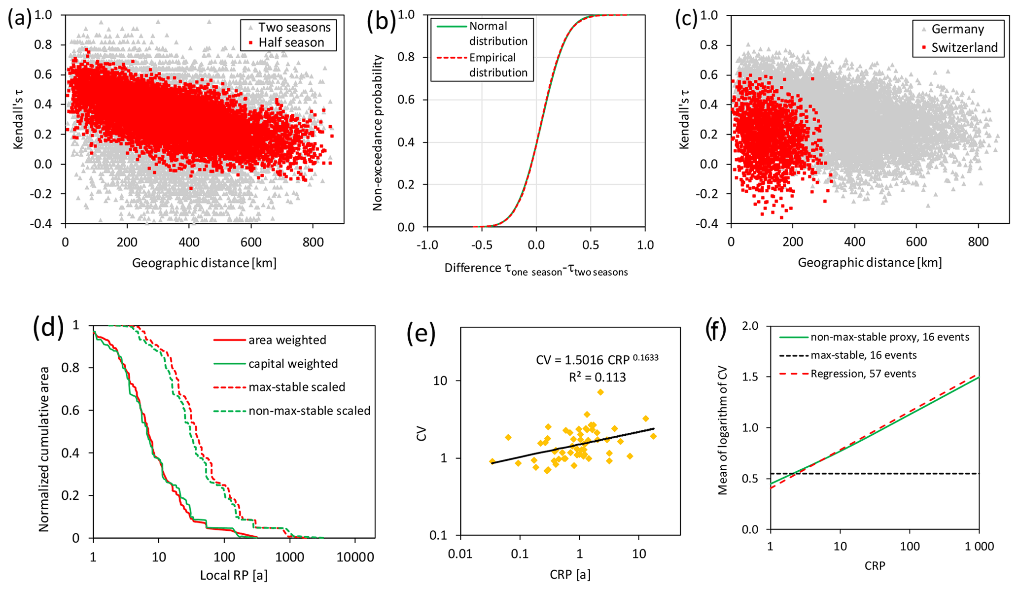
Figure 6 Spatial characteristics of winter storms over Germany: (a) estimated Kendall's τ versus distance, (b) differences between Kendall's τ for different block sizes, (c) estimated Kendall's τ versus distance for seasonal maxima in Germany and Switzerland (Raschke et al., 2011), (d) area functions for storm Kyrill with scaling to CRP 100 years, (e) relation CV to CRP of capital-weighted area functions, and (f) approximation of this relation by special stochastic scaling.

4.3 Spatial characteristics and dependence

As discussed in Sect. 2.4, the spatial characteristics is an important aspect from a stochastic perspective. Therefore, we have analyzed the relation between distance and dependence measure. We have applied Kendall's τ (Kendall, 1938; Mari and Kotz, 2001, Sect. 6.2.6) and show the dependence between the maxima of the half of a season and maxima of two seasons for 9870 pairs of stations in Fig. 6a. Since the sample size is relatively small, the spreading is strong; it is caused by estimation error.

Furthermore, the differences between the estimates of Kendall's τ for maxima of one and two hazard seasons are almost perfectly normally distributed (CDF in Fig. 6b) and should be centered to 0 in case of max stability (Fig. 2b). This does not apply with sample mean of 0.051 and standard deviation of 0.182. The corresponding normally distributed confidence range for the expectation has a standard deviation of 0.002 and a probability of 0.00 that the actual expectation is 0 or smaller.

For completeness, we compare the current estimates of Kendall's τ with those for Switzerland from Raschke et al. (2011) in Fig. 6c. The spatial dependence is higher for Germany. A reason might be differences in the topology.

We have also computed the area functions and show examples in Fig. 6d for winter storm Kyrill. The different weightings result in similar area functions. Figure 6e plots the CRP and CV of all events. The regression analysis reveals the statistical dependence between CRP and CV. For the linearized regression function, the p value is 0.002 (t test; Fahrmeir et al., 2013, Sect. 3.3). Due to two statistical indications of non-max-stability, we develop a local scaling that considers the global scaling factor and the ratio between local RP and CRP for every event with loss information. In this way, we could reproduce the observed pattern (Fig. 6f). Details of this workaround are presented in the Supplement data, Sect. 7. The differences between the scaling variants (max-stable or not) for storm Kyrill do not seem to be strong (Fig. 6d).

4.4 The risk estimates

Before we estimated risk curves according to the approach of Sect. 3.4, we must estimate a vulnerability function (Eq. 31) which determines the local loss ratio L_R in the event loss aggregation (Eq. 26). First, we fit the scaling parameter on the event loss data of the General Association of German Insurers (GDV, 2019) for 16 historical events from 2002 to 2018, as plotted in Fig. 7a. The details of the vulnerability function and its parameter fit are explained in Sect. 5.2. Then, we use the vulnerability function in the three variants of risk curve estimates of Sect. 3.4 – averaging event loss, CRP, or its reciprocal, the exceedance frequency. Details of the numerical procedure are explained in Sect. 5.3, which corresponds with the scheme in Fig. 4a.

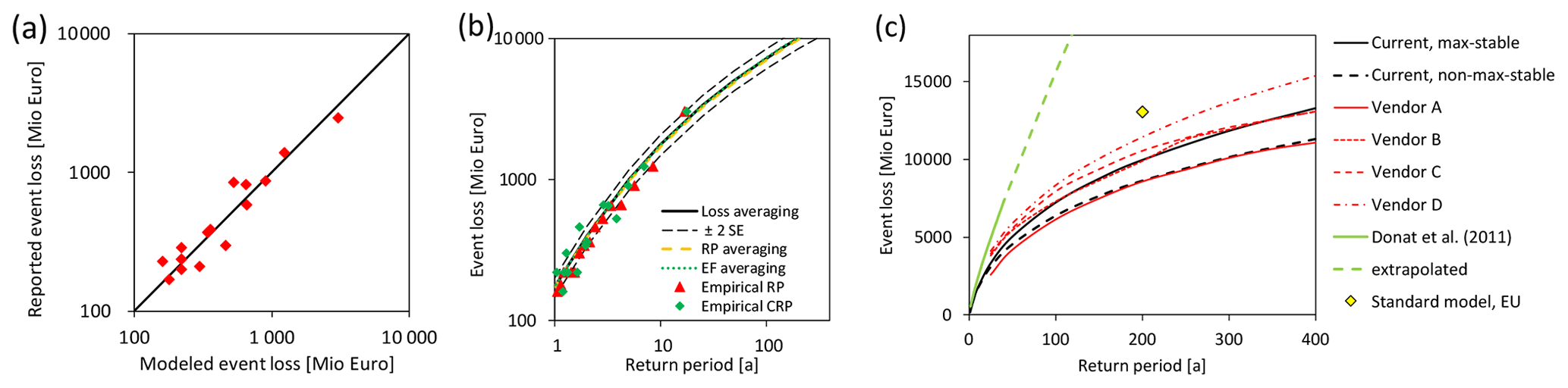
Figure 7 Estimates for insured losses from winter storms in Germany: (a) reported versus modeled event losses, (b) current risk curves and observations, and (c) influence of max-stable and non-max-stable scaling and comparison to scaled, previous estimates (Donat et al., 2011; Waisman, 2015; European Commission, 2014).

In Fig. 7b, the three estimated risk curves according to the three estimators in Eq. (28) are presented for max-stable scaling and differ less from each other, which indicates the robustness of our approach. The empiricism is presented by the historical event losses and their empirical RP (observation period 17 years of GDV loss data) and capital-weighted CRP. In addition, we present the range of two standard errors of the estimates of loss averaging which imply the simplest numerical procedure. Details of uncertainty quantification are explained in Sect. 5.4.

The differences between max-stable and non-max-stable scaling in the risk estimates are demonstrated in Fig. 7c. For smaller RP, no significant difference can be stated in contrast to higher RP. This corresponds with the differences between the CV in relation to the CRP for max-stable and non-max-stable cases in Fig. 6f. These are also higher for higher CRP.

We also compare our results with previous estimates in Fig. 7c. For this purpose, we must scale these to provide comparability as well as possible. The relative risk curve of Donat et al. (2011) is scaled simply by our assumption for the total sum insured (TSI) for the exposure year 2018. The vendor models of Waisman (2015) are scaled by the average of ratios between modeled and observed event losses from storm Kyrill since a scaling via TSI was not possible (uncertain market share and split between residential, commercial, and industry exposure). The result of the standard model of European Union (EU) regulations (European Commission, 2014), also known as Solvency II requirements, is also based on our TSI assumption, split into the CRESTA zones by the GAR data. The CRESTA zones (https://www.cresta.org/, last access: 12 October 2020) are an international standard in the insurance industry and correspond to the two-digit postcode zones in Germany.

The risk estimate of Donat et al. (2011) is based on a combination of frequency estimation and event loss distribution by the generalized Pareto distribution, which is fitted on a sample of modeled event losses for historical storms. The corresponding risk curve differs very much from other estimates and overestimates the risk of winter storms over Germany. The standard model of the EU only estimates the maximum event loss for RP of 200 years; the estimated event loss is very high. The vendor models vary but have a similar course as our risk curves. The non-max-stable scaling is in the lower range of the vendor models, whereas the unrealistic max-stable scaling is more in the middle. The concrete names of the vendors can be found in Waisman's (2015) publication. The reader should be aware that the vendors might have updated their winter storm model for Germany in the meantime.

The major result of Sect. 5 is the successful demonstration that the CRP can be applied to estimate reasonable risk curves under controlled stochastic conditions. In addition, we have discovered the strong influence of the underlying dependence model (max-stable or not) and the corresponding spatial characteristics to loss estimates for higher ELRP.

5 Technical details of the application example

5.1 Modeling and estimation of local hazard

As mentioned, the maximum wind gusts of half seasons of winter storms (extratropical cyclones) – block maxima – have been analyzed. Therein, the generalized extreme value distribution (Beirlant et al., 2004, Sect. 5.1) is applied:

$$\begin{array}{}\text{(29)}& \begin{array}{rl}& G\left(y\right)=\\ & \begin{array}{ll}\exp \left(-\exp \left(\frac{y-\mathit{\mu }}{\mathit{\sigma }}\right)\right),& \mathrm{if}\mathit{\gamma }=\mathrm{0}\\ \exp \left(-{\left(\mathrm{1}+\mathit{\gamma }\frac{y-\mathit{\mu }}{\mathit{\sigma }}\right)}^{-\mathrm{1}/\mathit{\gamma }}\right),& \mathrm{if}\mathit{\gamma }\ne \mathrm{0},\mathrm{with}y>\mathit{\mu }-\frac{\mathit{\sigma }}{\mathit{\gamma }}\\ & \mathrm{if}\mathit{\gamma }>\mathrm{0},\mathrm{and}\\ & y<\mathit{\mu }-\frac{\mathit{\sigma }}{\mathit{\gamma }}\mathrm{if}\mathit{\gamma }<\mathrm{0}\end{array}.\end{array}\end{array}$$

As discussed below, the Gumbel distribution (Gumbel, 1935, 1941), as a special case in Eq. (29) with extreme value γ=0, is an appropriate model. The scale parameter is σ, and the location parameter is μ. The local hazard function (Eqs. 13 and 14) can be derived directly from the estimated variant of Eq. (29) according to the link between extreme value distribution and exceedance frequency (Eq. 16) (the accent symbolizes the point estimation):

$$\begin{array}{}\text{(30)}& {\widehat{T}}_y\left(y\right)=\mathrm{1}/{\widehat{\mathrm{\Lambda }}}_y\left(y\right)=\exp \left({\displaystyle \frac{y-\widehat{\mathit{\mu }}}{{\widehat{\mathit{\sigma }}}_{\mathrm{cor}}}}\right).\end{array}$$

We apply the maximum likelihood (ML) method for the parameter estimation (Clarke, 1973; Coles, 2001, Sect. 2.6.3). The wind records' incompleteness per half season has been considered in the ML estimates by modifying the procedure as explained in the Supplement data, Sect. 5. A Monte Carlo simulation confirms the good performance of our modification. The biased estimate of σ for our sample size n=40 was also detected, in which we considered ${\widehat{\mathit{\sigma }}}_{\mathrm{cor}}=\widehat{\mathit{\sigma }}/\mathrm{0.98}$ as the corrected estimation. Landwehr et al. (1979) have already stated such bias. In addition, the exceedance frequency is well estimated by Eq. (30) in contrast to the RP $\widehat{T}$. The latter is strongly biased. We also corrected this as documented in the Supplement data, Sect. 6. The analyzed half-season maxima, record completeness, and parameter estimates are listed in the Supplement data, Tables 4–6.

We have validated the sampling of block maxima per half season. The opportunity of correlation between the first and second half-season maxima has been tested for significance level α=5 % and hypothesis H₀: uncorrelated samples. Around 6 % fail the test with Fisher's z transformation (Upton and Cook, 2008). This corresponds to the error of the first kind (Type I error, e.g., Lindsey, 1996, Sect. 7.2.3), the falsely rejected correct models. Therefore, we interpret the correlation as statistical insignificant. Similarly, the Kolmogorov–Smirnov homogeneity test rejects 4 % of the sample pairs for the period September to December and January to April (first half season to subsequent second half season) for a significance level of 5 %. There are no significant differences between the samples.

To optimize the intensity measure of the hazard model, we have considered the wind speed with power 1, 1.5, and 2 as the local event intensity in a first fit of the Gumbel distribution by the maximum likelihood method. According to these, power 1.5 offers the best fit of wind gust data to the Gumbel distribution. Such wind measure variants were already suggested by Cook (1986) and Harris (1996).

We do not apply the generalized extreme value distribution in Eq. (29) with extreme value index γ≠0 but the Gumbel case with γ=0 for the following reasons. Different stochastic regimes γ<0 and γ≥0 for different wind stations imply fundamental physical differences: finite and infinite upper bounds of wind speed. Such fundamental differences between different wind stations would need reasonable explanations (especially for very low bounds versus infinite bounds). River discharges at different gauging stations could imply such physical differences since there are variants with laminar and turbulent stream or very different retention/storage capacities of catchment areas (e.g., Salazar et al., 2012). Similar significant physical differences do not exist for wind stations that are placed and operated under consideration of rules of meteorology (World Meteorological Organization, 2008, Sect. 5.8.3) to provide homogeneous roughness conditions. Besides, we also found several statistical indications for our modeling. Akaike and Bayesian information criteria (Lindsey, 1996; here over all stations) indicate that the Gumbel distribution is the better model than the variant with a higher degree of freedom. Furthermore, the share of rejected Gumbel distributions of the goodness-of-fit test (Stephens, 1986, Sect. 4.10) is with 6 % around the defined significance level of 5 % (the error of the first kind – falsely rejected correct models). We have also estimated γ for each station and got a sample of point estimates. The sample mean is 0.002, very close to γ=0; this confirms our assumption. Moreover, the sample variance is 0.018 which is around the same as what we get for a large sample of estimates $\widehat{\mathit{\gamma }}$ for samples of Monte-Carlo-simulated and Gumbel-distributed random variables (n=40). All statistics validate the Gumbel distribution.

To provide reproducible results, we also present a computational example for the CRP in Table 1 with reference to all needed equations and information. The entire calculation for storm Kyrill is presented in the Supplement data, Table 8.

Table 1 Example for the computation of a CRP at Station #303 (Baruth) for storm Kyrill.

5.2 Modeling and estimation of vulnerability

To quantify the loss ratio L_R at location (wind station) j and event i in the loss aggregation (Eq. 26), we use the approach of Klawa and Ulbrich (2003) for Germany with a certain modification. The event intensity is the maximum wind gust speed v. v_98 % is the upper 2 % percentile from the empirical distribution of all local wind records. The relation with vulnerability parameter a_L is

$$\begin{array}{}\text{(31)}& L_{\mathrm{R},i,j}=a_{\mathrm{L}}\max {\left\{\mathrm{0},\left(v_{i,j}-v_{\mathrm{98}\mathit{\%}}\right)\right\}}^{\mathrm{3}}.\end{array}$$

Donat et al. (2011) have used a similar formulation but with an additional location parameter. This is discarded here since the loss ratio must be L_R=0 for local wind speed v<v_98 %. This is also a reason why a simple regression analysis (Fahrmeir et al., 2013) is not applied to estimate a_L. We formulate and use the estimator

$$\begin{array}{}\text{(32)}& {\widehat{a}}_{\mathrm{L}}={\displaystyle \frac{\mathrm{1}}{n}}\sum _{i=\mathrm{1}}^k{\displaystyle \frac{{\sum }_{j=\mathrm{1}}^n{E}_{j,i}\max {\left\{\mathrm{0},\left(v-v_{\mathrm{98}\mathit{\%}}\right)\right\}}^{\mathrm{3}}}{L_{\mathrm{E}\mathrm{reported},i}}},\end{array}$$

with k historical storms, corresponding reported event losses L_E, n wind stations, and local exposure value E_j,i being assigned to the wind station. E_j,i would be fixed for every station j if there were wind records for every storm i at each station j. However, the wind records are incomplete, and the assumed TSI must be split and assigned to the stations a bit differently for some storms. The exposure share of the remaining stations is simply adjusted so that the sum over all stations remains the TSI.

Our suggested estimator (Eq. 32) has the advantage that it is less affected by the issue of incomplete data (smaller events with smaller losses are not listed in the data) than the ratio of sums over all events, and the corresponding standard error can be quantified (as for the estimation of an expectation). The current point estimate is ${\widehat{a}}_{\mathrm{L}}=\mathrm{9.59}\times {\mathrm{10}}^{-\mathrm{8}}\pm \mathrm{5.97}\times {\mathrm{10}}^{-\mathrm{9}}$.

An example of our vulnerability function (with the average of v_98 % over the wind stations) is depicted in Fig. 8 and compared with previous estimates for Germany. It is in the range of previous models. Differences might be caused by different geographical resolutions of corresponding loss and exposure data. A power parameter of 2 in Eq. (31) might also be reasonable since the wind load of building design codes (EU, 2005, Eurocode 1) is proportional to the squared wind speed. The influence of deductibles (Munich Re, 2002) per insured object is not explicitly considered but smoothed in our approach.

Figure 8 Vulnerability functions: current estimate with the average of local parameters and previous estimates by Heneka and Ruck (2008) and Munich Re (2002) for residential buildings.

5.3 Numerical procedure of scaling

Here, we briefly explain the numerical procedure to calculate a risk curve via averaging the event loss. For any supporting point of a risk curve during an event loss averaging, the ELRP T_E is defined and determines the scaled CRP T_cs for all historical events. For each historical event, the scaling factor is $S=T_{\mathrm{E}}/T_{\mathrm{c}}$ according to Eq. (24) and is applied in Eq. (27) together with local hazard function (Eq. 30) and its inverse. The hazard parameters are listed in the Supplement data, Table 4. For the scaled local intensity, the local loss ratio L_R,i is computed with the vulnerability function (Eq. 31). The corresponding parameter v_98 % is also listed in the Supplement data, Table 2. The local loss ratio L_R,i and the local exposure value E_i are used in Eq. (26) to compute the event loss. The considered values of E_i per event are listed in the Supplement data, Table 7. The incompleteness of wind observation is considered therein. Finally, for the supporting point, the modeled event losses of all scaled historical events are averaged according to Eq. (28).

The historical events are also scaled for a defined event loss and the corresponding scaled CRP is averaged. However, the “goal seek” function in MS Excel is applied to find the correct scaled CRP T_sc and corresponding scaling factor S. For the averaging of the exceedance frequency, the reciprocal of T_sc is averaged. All these apply to max-stable scaling. For the non-max-stable scaling, the scaling factor S is adjusted to a local variant according to the description in the Supplement data, Sect. 7. Therein, the factor S is adjusted for each station and depends on the relation of local RP to CRP of the historical event. This adjustment is made for each historical storm individually.

5.4 Error propagation and uncertainties

The uncertainty of the local hazard models influences the accuracy of the CRP since the CRP is an average of estimates of local RP. The issue is that there is a certain correlation between the estimated hazard parameters of neighboring wind stations. We consider this by application of the jackknife method (Efron and Stein, 1981). According to these, the root of mean squared error (RMSE, which is the standard error if the estimate is bias free as we assume here) of the original estimated parameter $\widehat{\mathit{\theta }}$ is (accents symbolize estimations)

$$\begin{array}{}\text{(33)}& \mathrm{RMSE}\left(\widehat{\mathit{\theta }}\right)=\sqrt{{\displaystyle \frac{n-\mathrm{1}}{n}}\sum _{i=\mathrm{1}}^n{\left({\widehat{\mathit{\theta }}}_{-i}-\widehat{\mathit{\theta }}\right)}^{\mathrm{2}}},\end{array}$$

with the estimates ${\widehat{\mathit{\theta }}}_{-i}$ for the jackknife sample i of observations being the original sample but without one of the observations/realizations. Therefore, it is also called the leave-one-out method. The estimator (Eq. 33) implies a parameter sample of ${\widehat{\mathit{\theta }}}_{-i}$ of size n, with one estimated parameter or parameter vector for each jackknife sample i of observations.

To consider any correlation in the error propagation of CRP estimate, the maximum of the same half-season i is left out synchronously when the parameter sample is computed for each wind station. Without changing the order in the parameter sample of each wind station, the CRP ${\widehat{T}}_{\mathrm{c}-i}$ of the concrete historical event is computed with the hazard parameters ${\widehat{\mathit{\theta }}}_{-i}$ of each station. Finally, for this storm, the standard error of point estimate ${\widehat{T}}_{\mathrm{c}}$ is computed according to Eq. (33).

We use the same approach to consider the error propagation from local hazard models to the risk estimate for the max-stable case in Sect. 4.4. But the finally estimated parameter $\widehat{\mathit{\theta }}$ in Eq. (33) is the averaged event loss ${\widehat{L}}_{\mathrm{E}}\left(T_{\mathrm{E}}\right)$ for scaled CRP. This only covers a part of the uncertainties in the risk estimate. We consider two further sources of uncertainty and assume that they influence the risk estimate independently from each other. The uncertainty of loss averaging is the same as during an estimation of an expectation from a sample mean and is determined by sample variance and sample size (number of scaled events). The propagation of the uncertainty of the vulnerability parameter is computed via the delta method (Coles 2001, Sect. 2.6.4). The aggregated standard error is the square root of the sum of squared errors. This implies a simple variance aggregation according to the convolution of independent random variables (Upton and Cook, 2008).

The computed standard errors in Fig. 7b are in the range of 7.5 % to 8.5 % of estimated event loss per defined ELRP. The shares of uncertainty components on the error variance (squared SE) of our risk estimates depend on the RP. On average for our supporting point, these are 15 % for the limited sample of scaled historical events, 24 % for the uncertainty of local hazard parameters, and 61 % for the vulnerability model's parameter. Unfortunately, we do not know a published error estimation for a vendor model for winter storm risk in Germany. Therefore, we can only compare our estimates with Donat et al.'s (2011). Their confidence range indicates a smaller precision than ours.

5.5 RP of vendor's risk estimate

We have compared our results with vendor models in Sect. 4.4. These have estimated the risk curve for the maximum event loss within a year. This is a random variable, and their RP is the reciprocal of the exceedance probability and can never be smaller than 1. We transform the RP of annual maxima to the RP of event loss according to the relations in Sect. 3.1 and the explanations by Coles (2001, p. 249, with y_p as exceedance frequency of events). The relative differences between the RPs are around 5 % for ELRP of 10 years and 0.5 % for ELRP of 100 years.

6 Conclusion, discussion, and outlook

6.1 General

In the beginning, we asked the questions about the RP of a hazard event in a region, the corresponding NatCat risk, and necessary conditions for a reasonable NatCat modeling. To answer our questions, we have mathematically derived the CRP of a NatCat-generating hazard event from previous concepts of extreme value theory, the pseudo-polar coordinates (Eq. 17). This implies the important fact that the average of the RPs of random point events remains a RP with exceedance frequency (Eqs. 8 and 15). Furthermore, we extended Schlather's first theorem for max-stable random fields to the non-max-stable spatial dependence and characteristics. We have also considered the normalized variant of the area function of all local RPs of the hazard event in a region with parameters CRP and CV. The absence of max-stability in the spatial dependence results in a correlation between CRP and CV, which is a further indicator for non-max-stability beside changes in measures for spatial dependence by changed block size (e.g., annual maxima versus 2-year maxima).

The derived CRP is a universal, simple, plausible, and testable stochastic measure for a hazard and NatCat event. The weighting of local RP in the computation of the CRP can be used to compensate for an inhomogeneous distribution of corresponding measuring stations if the physical-geographical hazard component of a NatCat, the field of local event intensity, is of interest. However, the concentration of human values in the geographical space could also be considered in the weighting to obtain a higher association of the CRP with the ELRP of a risk curve. This link implies the conditional expectation (Eq. 18) under the assumption of a max-stable association between CRP and ELRP and offers a new opportunity to estimate risk curves, the bijective function event loses to ELRP, via a stochastic scaling of historical intensity fields and averaging of corresponding risk parameter. The averaged parameter can be the scaled CRP for a defined event loss, corresponding exceedance frequency, or the event loss for a defined/scaled CRP.

The differences between the three estimators are small in our application example, insured losses from winter storms over Germany. In contrast, the influence of the stochastic assumptions regarding the spatial dependence and characteristics (max-stable or not) is significant in the range of higher ELRPs. This highlights the importance of a realistic consideration of the spatial dependence and characteristics of the hazard in a NatCat model. Besides, our risk curves for Germany have a similar course as those derived by vendors (Fig. 7d). The risk assumption by the EU for Germany with ELRP of 200 years is significantly higher than ours. The estimate by Donat et al. (2011) differs significantly and seems to be implausible for higher ELRP. A reason might be their statistical modeling by the generalized Pareto distribution as already applied for wind losses by Pfeifer (2001). The tapered Pareto distribution (Schoenberg and Patel, 2012), also called tempered Pareto distribution (Albrecher et al., 2021), or a similar approach (Raschke, 2020) provide more appropriate proxies for our risk curve's tail.

According to our results, necessary conditions for appropriate NatCat modeling are the realistic consideration of local hazard and their spatial dependence (max-stable or not?). Correspondingly, the spatial characteristics of NatCat events, described here by relation CRP to CV, must be reproduced. In addition, the CRPs of a simulated set of hazard events in a NatCat model should have an empirical exceedance frequency that follows the theory (Eq. 15). Finally, the standard error of an estimate should be quantified, the sampling should be appropriate, and overfitting (over parametrization and parsimony) should be avoided. This principle applies to all scientific models with a statistical component (e.g., Lindsey, 1996).

The advantage of our approach over vendor models is the simplicity and clarity of the stochastic assumptions. The numerical simulations for models in the insurance industry (Mitchell-Wallace et al., 2017, Sect. 1.8) and science (e.g., Della-Marta et al., 2010) need tens of thousands of simulated storms with unpublished or even unknown (implicit) stochastic assumptions. We have only scaled 16 event fields of historical storms with controlled stochastics and could even quantify the standard error.

6.2 Requirements of the new approaches

Our approach to CRP is based on two assumptions. At first, the local and global events occur as a Poisson process. This is a common assumption or approximation in applied extreme value statistics (Coles, 2001, Sect. 7), and the corresponding Poisson distribution of the number of events can be statistically tested (Stephens, 1986, Sect. 4.17). Moreover, the verified clustering (overdispersion) of winter storms over Germany (Karremann et al., 2014) is statistically not relevant for higher RP (Raschke, 2015a). With increasing RP, the number of winter storms occurring converges to a Poisson distribution. Clustering is also influenced by the event definition, which is not the topic here (keyword declustering; Coles, 2001). We also point out that the assumed Poisson process does not need to be homogenous during a defined unit period (year, hazard season, or half season).

The second prerequisite is robust knowledge about the local RP by a local hazard curve. Unfortunately, there are no appropriate and comprehensive models for the local hazard of every peril and region, for example, hail in Europe; we only know local hazard curves for Switzerland by Stucki and Egli (2007), and these were roughly estimated. There are public hazard maps of flooding areas for defined RP; corresponding local hazard curves are rarer.

Furthermore, existing models for local hazard are partly questionable according to our discussion about local modeling of wind hazard from winter storms in Sect. 5.1. We have assumed a Gumbel case of the generalized extreme value distribution for local block maxima with extreme value index γ=0 for several statistical indicators and physical consistency. Youngman and Stephenson's (2016) modeling of winter storms over Europe implies an extreme value index γ<0 for the region of Germany, which means a short tail with a finite upper bound. They have not depicted the spatial distribution of the corresponding finite upper bounds and do not provide a physical explanation for the spatially varying upper physical limit of wind speed maxima. The plausibility of such physical details in a NatCat model should be shown and discussed.

6.3 Opportunities for future research

Since the current model for the local hazard of winter storms over Germany results in considerable uncertainty, it should be improved in the future. This could be realized by a kind of regionalization of the hazard as already known in flood research (Merz and Blöschl, 2003; Hailegeorgis and Alfredsen, 2017) or a spatial model (Youngman and Stephenson, 2016). Besides, more wind stations could be considered in the analysis with better consideration of incompleteness in the records. An extension of the observation period is conceivable if homogeneity of records and sampling is ensured. A more sophisticated approach might be used to discriminate the extremes of winter storms from other windstorm perils at the level of wind station records. The POT methods (Coles, 2001, Sect. 4.3; Beirlant et al., 2004, Sect. 5.3) could then be used in the analysis even though the spatial sampling is complicated as stated in the “Introduction”.

Further opportunities for improvements in the winter storm modeling are conceivable. The event field might be reproduced/interpolated in more detail, as done by Jung and Schindler (2019). They have considered the roughness of land cover at a regional scale besides further attributes. However, they did not consider the local roughness of immediate surroundings, as Wichura (2009) discussed for a wind station.

Besides, our approach could be used for further hazards such as earthquake, hail, or river flood. The reasonable weighing would not be trivial for river flood. It may be that the local expected annual flood loss would be a reasonable weighting if the final goal is a risk estimate for a region. The numerical handling of the case that an event does not occur everywhere in the researched region but local RP T=0 must be discussed for some perils, such as hail or river flood.

We also see research opportunities for the community of mathematical statistics, especially extreme value statistics. Does Eq. (18) for conditional expected RP also apply to the non-max-stable case? A deeper theoretical understanding of non-max-stable random fields with max-stable margins is of great interest from practitioners' perspectives. Research about the link between normalized area functions (expectation versus CV) and spatial dependence could increase understanding of natural hazard and risk, and our construction for the non-max-stable scaling is just a workaround to illustrate the consequences of dependence characteristics; for risk models in practice, a transparent stochastic construction is needed. Furthermore, estimation methods could be extended and examined, such as the bias in estimates of local RP.