On the correlation between a sub-level qualifier refining the danger level with observations and models relating to the contributing factors of avalanche danger

Forecasting avalanche danger at a regional scale is a largely data-driven yet also experience-based decision-making process by human experts. In the case of public avalanche forecasts, this assessment process terminates in an expert judgment concerning summarizing avalanche conditions by using one of five danger levels. This strong simplification of the continuous, multi-dimensional nature of avalanche hazard allows for efficient communication but inevitably leads to a loss of information when summarizing the severity of avalanche hazard. Intending to overcome the discrepancy between determining the final target output in higher resolution while maintaining the well-established standard of assessing and communicating avalanche hazard using the avalanche danger scale, avalanche forecasters at the national avalanche warning service in Switzerland used an approach that combines absolute and relative judgments. First, forecasters make an absolute judgment using the five-level danger scale. In a second step, a relative judgment is made by specifying a sub-level describing the avalanche conditions relative to the chosen danger level. This approach takes into account the human ability to reliably estimate only a certain number of classes. Here, we analyze these (yet unpublished) sub-levels, comparing them with data representing the three contributing factors of avalanche hazard: snowpack stability, the frequency distribution of snowpack stability, and avalanche size. We analyze both data used in operational avalanche forecasting and data independent of the forecast, going back 5 years. Using a sequential analysis, we first establish which data are suitable and in which part of the danger scale they belong by comparing their distributions at consecutive danger levels. In a second step, integrating these findings, we compare the frequency of locations with poor snowpack stability and the number and size of avalanches with the forecast sub-level. Overall, we find good agreement: a higher sub-level is generally related to more locations with poor snowpack stability and more avalanches of larger size. These results suggest that on average avalanche forecasters can make avalanche danger assessments with higher resolution than the five-level danger scale. Our findings are specific to the current forecast set-up in Switzerland. However, we believe that avalanche warning services making a hazard assessment using a similar temporal and spatial scale as currently used in Switzerland should also be able to refine their assessments if (1) relevant data are sufficiently available in time and space and (2) a similar approach combining absolute and relative judgment is used. The sub-levels show a rank-order correlation with data related to the three contributing factors of avalanche hazard. Hence, they increase the predictive value of the forecast, opening the discussion on how this information could be provided to forecast users.

1 Introduction

In many snow-covered mountain regions, avalanche forecasts are disseminated to the public to inform and warn about avalanche conditions. The provision of these warnings to the public consists of two steps: first, a prediction of the avalanche hazard is made, and, second, the prediction is communicated in a forecast product.

Assessing and forecasting avalanche hazard is a largely empirical process in which a human forecaster analyzes and interprets data to make an informed judgment regarding current or expected avalanche conditions (e.g., LaChapelle, 1980; McClung, 2002; Floyer et al., 2016). During the hazard assessment process the following four questions – what is the avalanche problem, where and when does it exist, how likely is it that an avalanche will occur, and how big will the avalanche be – must be answered (Statham et al., 2018a). This requires assessing the three factors contributing to avalanche hazard for each identified avalanche problem (Fig. 1a;  Techel et al., 2020a; EAWS, 2021).

• Snowpack stability describes the stability of the snowpack at a point (Techel et al., 2020a). Snowpack stability is inversely related to the probability of avalanche release. It is also referred to as the sensitivity to triggers (conceptual model of avalanche hazard, CMAH; Statham et al., 2018a), which assesses the sensitivity of the snowpack to fail given a specific triggering level (Statham et al., 2018a), as for instance a person skiing a slope.

• The frequency distribution of snowpack stability describes the respective proportions of spots where triggering an avalanche given a specific triggering level is possible (Techel et al., 2020a; EAWS, 2021). It is also referred to as the “spatial distribution” (Statham et al., 2018a). The sensitivity to triggers and the spatial distribution describe the likelihood of avalanches in the CMAH.

• Avalanche size refers to the destructive potential of avalanches.

Once all relevant avalanche problems have been identified, their location and temporal occurrence specified, and their character described, avalanche hazard is summarized in regional avalanche forecasts using one of five danger levels (see Fig. 1b) according to a danger scale (i.e., in Europe the European Avalanche Danger Scale, EADS; EAWS, 2020). Aspects and elevation ranges where the danger and/or where the avalanche problems prevail are highlighted in the forecast products. Hence, a human forecaster reduces the avalanche conditions, continuous and multi-dimensional in nature, to a set of symbols (levels, classes, terms, text) representing this reality (LaChapelle, 1980; Hutter et al., 2021). As pointed out by Murphy (1993), the description of a continuous phenomenon using a discrete number (or level) inevitably leads to a loss of information. Forecasters attempt to bridge this gap between a continuous phenomenon and a discrete level using the narrative part of the avalanche forecast (e.g., Hutter et al., 2021). Regardless, a coarse resolution may lead to considerable differences within a (spatial or temporal) unit or a class (e.g., within a danger level;  SLF, 2020). It is therefore important that avalanche forecasters assess avalanche danger as detailed as possible when preparing a public forecast, given the available data and resources. This level of detail may be greater than what is communicated in the forecast product (e.g., Walcher et al., 2018; Techel et al., 2020b).

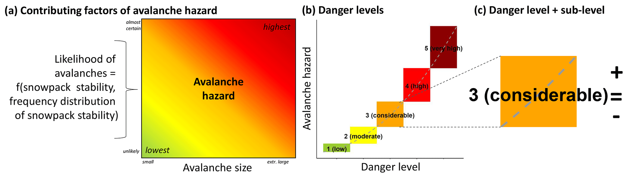
Figure 1 (a) Avalanche hazard chart. The contributing factors of avalanche hazard are snowpack stability, the frequency distribution of snowpack stability, and avalanche size (Techel et al., 2020a; EAWS, 2021). In the CMAH, these are termed the likelihood of triggering and the destructive avalanche size (Statham et al., 2018a). (b) Avalanche hazard, continuous in nature, is summarized using five ordinal danger levels. (c) In Switzerland, three ordinal sub-levels are assigned to danger levels indicating whether the hazard is high (+ or plus), in the middle (= or neutral), or low (− or minus) within a respective level. The gradient of the color transition (panel a) and the shape of the curve and the size of the boxes in panel (b) are for illustration purpose only.

An increased level of detail may include, for instance, decomposing the judgmental forecasting process and specifying each of the individual components relevant for the final hazard assessment (MacGregor, 2001; Statham et al., 2018a). It may, however, also entail increasing the resolution of the hazard assessment either in a spatial or temporal context, with regard to assessing the individual components of avalanche hazard, or of avalanche danger itself. Increasing the temporal and spatial resolution primarily requires sufficient relevant and new data in time and space, as well as the resources to efficiently analyze these data. In contrast, increasing the resolution of the danger scale to greater than the existing five levels requires clear definitions of these levels. Furthermore, making judgments on a scale with many options contrasts with the well-established finding that absolute judgments on a scale with more than seven points become unreliable (Miller, 1956). However, alternatively, a two-step approach can be used, which combines absolute and comparative judgments (Goffin and Olson, 2011; Kahneman et al., 2021): following such an approach, a first assessment is made using a small number of categories relying on guidelines or definitions. In the case of avalanche forecasting, this could be the step to assign a danger level according to the five-level avalanche danger scale (EAWS, 2018). In a second step, a relative rating is made with regard to this level (Kahneman et al., 2021). Compared to absolute judgments, this approach requires more effort and is time-consuming but allows a finer discrimination within previously assigned categories (Kahneman et al., 2021). Such an approach has been used during the past 5 years in Switzerland, where forecasters assigned a danger level and a sub-level qualifier refining where within this danger level the avalanche conditions are expected (Techel et al., 2020b). This leads to our over-arching research question: using such an approach to assign a sub-level qualifier to a danger level, can human avalanche forecasters forecast avalanche hazard at finer granularity than the five danger levels?

Unfortunately, addressing this question is not straightforward as avalanche danger and, hence, the sub-levels cannot be measured. However, since the danger levels represent a rank order in terms of the severity of the avalanche conditions, we tackle this question using a comparative approach testing whether there is a positive monotonic correlation between the sub-levels assigned to danger levels and data describing the three contributing factors of avalanche hazard. Specifically, we investigate whether there is a rank order relationship between the data and the sub-levels. For this, we make use of both observational data collected for the purpose of avalanche forecasting in Switzerland and independent data sources not used in the forecasting process: the output from two recently developed models (Pérez-Guillén et al., 2021; Mayer et al., 2022) and data related to avalanche risk (Winkler et al., 2021).

We first determine for each parameter in what range of the danger scale it correlates with the forecast danger levels (D). Here, we assume that the forecast danger level is correct on average, which has been shown for Switzerland (e.g., Techel and Schweizer, 2017; Schweizer et al., 2021) but also for other forecasts (e.g., Logan and Greene, 2018; Statham et al., 2018b). If a correlation exists, and given that the sub-levels (D_sub) are used consistently, we can expect a correlation between the sub-levels (D_sub) and the data as well. Therefore, in this study, we ask the following two research questions.

1. Does a data source representing a contributing factor of avalanche hazard correlate with the danger level D? If so, in which range of the danger scale?

2. For the range in the danger scale determined in (1), is there a monotonically increasing correlation between the parameter representing a contributing factor and the sub-levels D_sub as well?

2 Avalanche forecast in Switzerland – brief overview and approach to assign a sub-level qualifier to the danger level

The Swiss avalanche forecast has previously been described in several publications (Techel and Schweizer, 2017; SLF, 2020; Hutter et al., 2021). Here, we therefore only summarize some key facts.

Figure 2 Maps of Switzerland showing (a) the avalanche forecast published on 10 March 2018 and (b) the (unpublished) sub-levels for this forecast. In addition, the warning regions, the smallest spatial units used in the Swiss forecast, are shown as polygons with grey outlines in (b). These are aggregated to danger regions in the published forecast (i.e., region A in a).

During winter, the national avalanche warning service at the WSL Institute for Snow and Avalanche Research SLF (SLF) publishes an avalanche forecast at 17:00 LT (local time), valid until 17:00 LT the following day (see example in Fig. 2a). This forecast is updated at 08:00 LT during the main winter season. Definitions and guidelines provided by the European Avalanche Warning Services (EAWS) are used when assessing and communicating avalanche danger. A team of eight forecasters is involved in the production of the forecasts.

The production of the forecast always starts with the assessment of the current avalanche conditions. Numerous data are used in this process. These include measurements from automated weather stations located at the elevation of potential avalanche starting zones (SLF, 2022), simulations from the physical snow-cover model SNOWPACK (Lehning et al., 2002) driven with these measurements, and observational data collected for the purpose of avalanche forecasting. For the actual forecast, forecasters primarily use the numerical weather prediction model COSMO with 1 km resolution (MeteoSwiss, 2022). The three forecasters together on duty individually draw up their hazard assessment for the entire forecast domain. In a group discussion at the forecaster briefing, these assessments are combined resulting in one consolidated forecast for the following 24 h forecast period.

The Swiss avalanche forecast describes regional avalanche conditions. The average size of the almost 150 warning regions, the smallest spatial units used in the forecast, is about 200 km² (grey polygons in Fig. 2b). However, depending on conditions, these warning regions are flexibly aggregated to danger regions (i.e., region A in Fig. 2a) where avalanche conditions are considered similar, and they are described with the same danger level, critical aspects, and elevations where the danger prevails, as well as avalanche problems and danger description. In addition, since the winter of 2016/2017 forecasters assess where within a danger level the avalanche conditions are expected. To do so, an approach combining absolute and comparative judgments, as described in the previous section, is used. Forecasters first assign a danger level according to the definitions in the EADS and then make a comparative refinement using one of three qualifier terms (Techel et al., 2020b):

• plus or +: the danger is assessed as high within the level; e.g., a 3⁺ is high within 3 (considerable);

• neutral or =: the danger is assessed as being about in the middle of the level; e.g., a 3⁼ is about in the middle of 3 (considerable);

• minus or −: the danger is assessed as low within the level; e.g., a 3⁻ is low within 3 (considerable).

In the following, we refer to the danger levels (D) by integer signal word, i.e., 3 (considerable), and to the sub-levels (D_sub) by the integer qualifier, i.e., 3⁺.

Note that the criteria to distinguish between sub-levels and the range covered by a sub-level within a danger level remained undefined. Furthermore, forecasters made no such differentiation for 1 (low), as a further distinction within this level seemed impossible. In addition, an internal analysis of qualifiers assigned to danger levels describing wet-snow conditions showed that forecasters primarily assigned the sub-level plus to 2 (moderate) and 3 (considerable). Hence, for wet-snow conditions, the assignment of sub-level qualifiers was halted after a test winter.

Table 1 Overview showing the analyzed data sources and the contributing factors of avalanche hazard (snowpack stability, the frequency of snowpack stability, avalanche size) for which we consider the respective data sources to be a proxy. x refers to a contributing factor which was analyzed, and (x) to a factor which is included in the variable but does not vary (i.e., for natural avalanches the stability class (type of trigger) is constant and thus natural release).

3 Data description and preparation

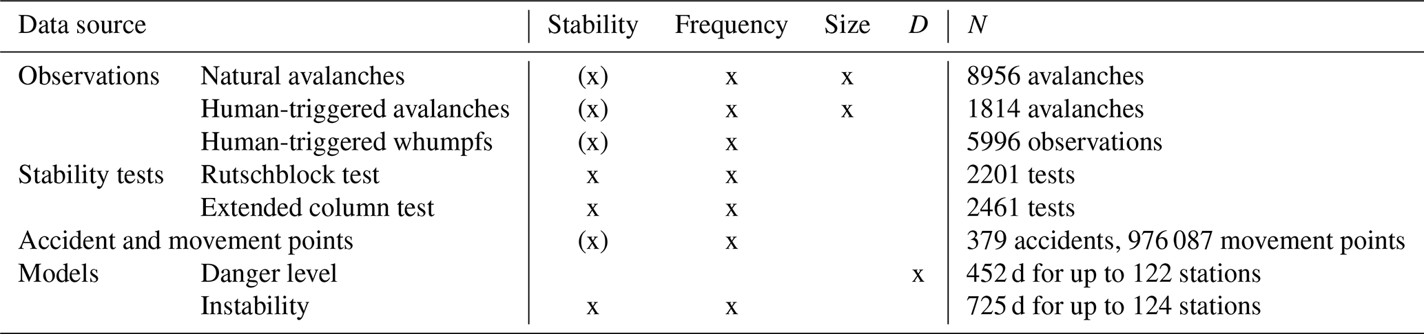
We analyzed observational data collected as part of our operational avalanche forecasting (Sect. 3.2). If available at the time when forecasters produced the forecast for the following day, these observations were considered by forecasters in the assessment of the current avalanche conditions. Moreover, we also used external data and two recently developed models which were not available during the forecast process (Sects. 3.3 and 3.4). Data from five winters 2016/2017 to 2020/2021 were used; for the danger-level model (Sect. 3.4.1) only data from winters 2018/2019 to 2020/2021 were available.

In the following, we describe the data and their preparation for this analysis.

3.1 Avalanche forecast

We extracted the forecast danger level, the unpublished sub-level, and the critical aspects and elevations, referred to as the core zone (Fig. 2a and b), that described dry-snow conditions in the Swiss Alps. Forecasts describing exclusively wet-snow or gliding avalanches as the main avalanche problem were excluded as no sub-level was assigned (Sect. 2). We used the forecasts issued at 17:00 LT, valid until the following day at 17:00 LT. These forecasts were published on 832 d.

3.2 Observations

3.2.1 Avalanche observations

The occurrence of avalanches directly indicates instability (e.g., McClung and Schaerer, 2006). Avalanche occurrence data can provide information on all three contributing factors (Table 1): snow instability (i.e., an avalanche released naturally), the frequency of unstable locations (i.e., the number of naturally released avalanches), and avalanche size (Schweizer et al., 2020).

In Switzerland, about 80 “stationary” observers report avalanches in their region on a daily basis. Observers report avalanches either individually or by aggregating avalanches into an avalanche summary report. In addition to avalanches regularly reported by these observers, field observers, who are also part of the observer network, and the public may report avalanches. Reported avalanche properties include the location and the estimated time of the release, the avalanche size (size classes 1 to 5 according to EAWS, 2019), the moisture content (dry or wet), and the trigger type (i.e., natural release, human-triggered;  SLF, 2020). Observers also indicate when there was no avalanche.

Natural avalanches. We extracted all avalanches of size 2 or larger with trigger type natural release. We excluded avalanches classified as a wet-snow or gliding avalanche. Moreover, we reduced the data set to consider only the 20 % of the warning regions with the highest number of days with at least one dry-snow avalanche. We considered a high number of days with reported avalanches as an indicator for regular observations. Consequently, we expected that the number of days with no avalanches due to missing observations or wrong dating of avalanches is reduced, and hence the quality of the avalanche observations is increased. These warning regions are marked in Appendix Fig. A1a. In total, 8956 avalanches fulfilled these criteria. In addition, observers reported no avalanches in 8826 cases.

Human-triggered avalanches. For human-triggered avalanches, of which a large share is reported by rescue services and the public, we considered reported events when the trigger type was human-triggered, when the avalanche size was size 2 or larger or when a person was caught in the avalanche, and when the avalanche was not classified as a wet-snow or gliding avalanche. For the purpose of this analysis, we assigned size class 2 if a size estimate was missing, which was the case for 151 of the 603 accidental avalanches but also for the 23 accidental avalanches classified as size 1. In total, 1814 human-triggered avalanches were considered in this analysis (their spatial distribution is shown in Appendix Fig. A1b). These were triggered during backcountry touring (i.e., during a ski or snowshoe tour) or during riding in unsecured avalanche terrain close to ski areas.

3.2.2 Human-triggered whumpfs and shooting cracks

Whumpfs, a sudden, collapse-type failure of a weak layer due to rapid localized loading (Schweizer and Jamieson, 2010), as, for instance, by a human, and shooting cracks in the snowpack provide an indication of the presence of locations potentially prone to being triggered by a human (Table 1).

When reporting their observations after a day in the field, observers also report whether they observed human-triggered whumpfs and shooting cracks and how frequent these danger signs occurred using three classes (DS.class): none (0 such observations), rare (1 to 3 such observations), and frequent (> 3 observations;  SLF, 2020).

We extracted all observations which were reported after a day in the field. This resulted in 5996 observations.

3.2.3 Stability tests

Information on snowpack stability can also be obtained by digging a snow pit and performing a stability test. These tests primarily provide very localized information on snowpack stability. Therefore, to obtain information on the frequency distribution of snowpack stability, numerous tests must be performed on the same day and in the same region (e.g., Birkeland, 2001; Schweizer et al., 2003). Alternatively, tests obtained under similar avalanche conditions may be combined to derive typical stability distributions (Techel et al., 2020a).

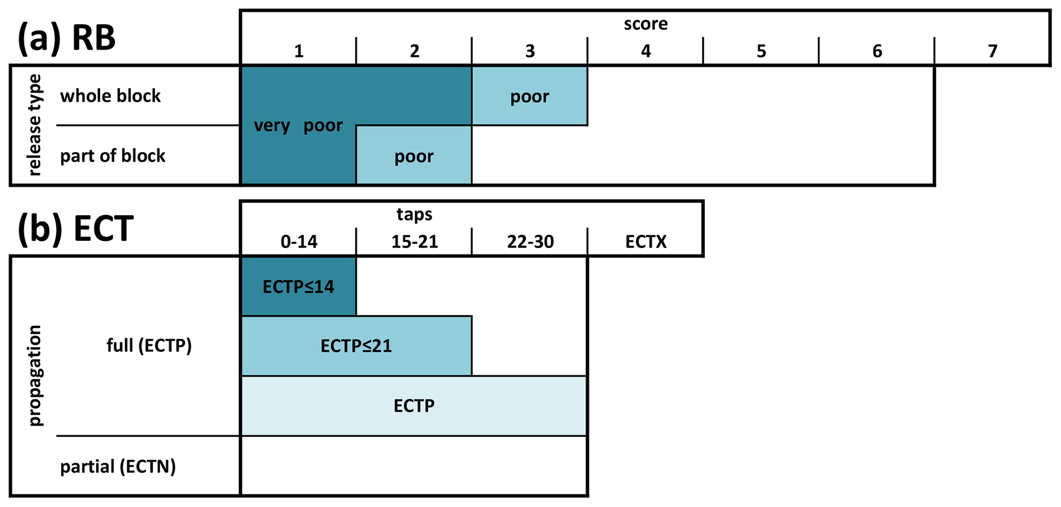
Figure 3 Classification of stability tests: (a) Rutschblock (RB) and (b) extended column test (ECT). The RB classification (RB.class) considers the score (seven loading steps) and the release type (whole block and part of block including release type edge only). Similarly, ECTs are classified combining the number of taps to initiate a fracture (30 loading steps) and the propagation propensity (full propagation: ECTP; partial or no propagation: ECTN). RB score 7 and ECTX indicate that no failure could be initiated following loading.

In Switzerland, two stability tests are performed regularly by observers to assess snowpack stability: the Rutschblock test (RB;  Schweizer, 2002; SLF, 2020) and the extended column test (ECT;  Simenhois and Birkeland, 2009; SLF, 2020). With these tests, the stability of an isolated block of snow is tested by loading the block according to the defined loading steps by a human (RB) or by tapping with the hand on a shovel blade lying on top of the snow column (ECT) until a fracture in the column is observed. The interpretation of the test results considers the type of release (i.e., fracture across the entire block or only part of the block) and the loading step. For an overview and comparison of the two tests refer to Techel et al. (2020c).

Rutschblock (RB). We classified the RB results according to the classification by Techel et al. (2020a) into four stability classes (RB.class: very poor, poor, fair, good). However, in this analysis, we considered exclusively the two classes very poor and poor (Fig. 3a) as these are most closely linked to unstable conditions (Schweizer and Jamieson, 2010; Techel et al., 2020c).

Extended column test (ECT). We treated a test result as potentially unstable if a fracture propagated within one tap across the whole column (ECTP;  Winkler and Schweizer, 2009). In addition, fracture propensity was combined with three different fracture initiation criteria as suggested in previous studies (Simenhois and Birkeland, 2009; Winkler and Schweizer, 2009; Techel et al., 2020c). The corresponding three stability classes are shown in Fig. 3b.

In total, 2201 RB and 2261 ECT were available. Their spatial distribution is shown in Fig. A1c in the Appendix.

3.3 Accidental avalanches and backcountry touring activity

Recently, Winkler et al. (2021) analyzed avalanche risk during backcountry touring in Switzerland. In their analysis, Winkler et al. relied on a data set of accident points extracted from the accident database at SLF and movement points in potential avalanche terrain extracted from GPS tracks recorded during backcountry ski tours in Switzerland (Schmudlach, 2021). Avalanche risk, as defined by Winkler et al. (2021), is the ratio of events (accident points) to events and non-events (accident and movement points combined) after backcountry users have adapted their behavior to the conditions. This ratio is closely related to the density of locations where triggering of an accidental avalanche by a human is possible and, thus, in a more general way also to the density of potential triggering locations (Table 1).

We relied on an updated version of the data set used by Winkler et al. (2021), including the two most recent winters 2019/2020 and 2020/2021. We filtered the data according to the specification by Winkler et al. (2021) which keeps points located in potential avalanche terrain. This approach to classifying avalanche terrain considers a relevant slope area for each point in the terrain. Therefore, points lying in avalanche release areas but also in slopes below may be considered avalanche terrain (for details refer to Schmudlach and Köhler, 2016; Schmudlach et al., 2018). In total, the data set contains 379 avalanche accident points and 976 087 movement points extracted from 2519 individual GPS tracks.

3.4 Models (random forest classifiers) based on snow-cover simulations

In addition to observational data, we analyzed the output of two recently developed random forest classifiers predicting the danger level (Pérez-Guillén et al., 2021) or snow-cover instability (Mayer et al., 2022). Both models use snow-cover simulations from the operational SNOWPACK model (Lehning et al., 2002) driven with data from 124 automatic weather stations as input (Lehning et al., 1999; Morin et al., 2019). An overview of the spatial distribution of these stations is provided in Appendix Fig. A1d. These stations are situated at the elevation of potential avalanche starting zones. In addition to simulations for flat study plots, snow-cover simulations are operationally made for virtual slopes with a slope incline of 38^∘ and the four slope orientations N, E, S, and W (Morin et al., 2019). During the explored winter seasons, these two random forest models were not used during the forecast production process.

3.4.1 Danger-level model

The first model, which we refer to as the danger-level model, was trained with a large data set of quality-checked danger levels spanning more than 20 years (Pérez-Guillén et al., 2021). The random forest classifier (Breiman, 2001) uses 30 features, describing both measured meteorological conditions (24 h averaged values) and snow-cover properties simulated with the SNOWPACK model. The random forecast classifier provides the probabilities (“prob”) for the four danger levels, 1 (low) to 4 (high), relying on an ensemble of 1000 classification trees. We used the model predictions relying on daily average weather variables and features extracted from the simulated snow stratigraphy at 12:00 LT on the day of interest. In total, model output was available for 452 d and at 122 stations for simulations made for the four virtual slope orientations N, E, S, and W.

3.4.2 Instability model

The second model developed by Mayer et al. (2022) – we refer to it as the instability model – also uses snow-cover simulations provided by the SNOWPACK model to assess snow instability. The instability model uses six variables describing the potential weak layer and the overlying slab to predict the probability prob_unstab that a snow layer is unstable. Based on an ensemble of 400 classification trees, the output probability ranges from 0 (a layer was classified as stable by all the trees) to 1 (all trees classified it as unstable). We used the simulated snow stratigraphy at 12:00 LT on the day of interest, considering the same simulations for the virtual slopes as for the danger-level model. Model output was available on 725 d and for up to 124 automatic weather stations.

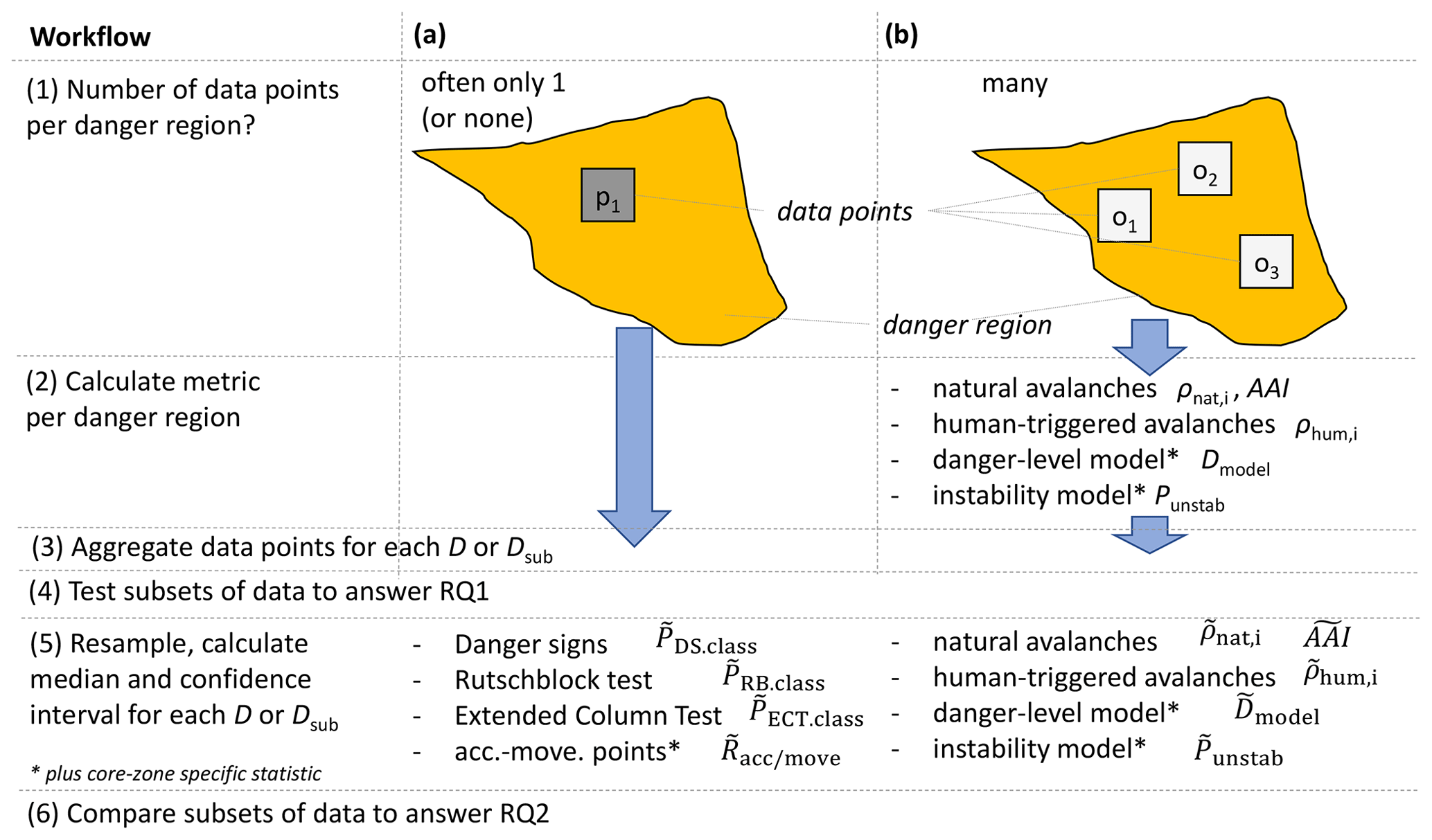
Figure 4 Workflow: preparatory steps (steps 1 to 3) and analysis to answer research question 1 (step 4) and 2 (steps 5 and 6).

4 Methods

4.1 Definition of parameters

We linked the forecast with the observations and the model output by their location and calendar day.

For this analysis, we distinguished between

1. data sources which mostly included only a single data point or even no data at all per forecast danger region (Fig. 4a – step 1) and

2. data which allowed the calculation of a proportion or a mean for each forecast danger region (Fig. 4b).

The first group included observations of danger signs, stability test results, and the accident and movement points, while the second group contained observations of natural and human-triggered avalanches and the predictions of the two models.

For the data sources with sufficient data points per danger region, we defined the following parameters that summarize the observations or modeled output for a given danger region (i.e., for the danger region A in Fig. 2a). This step is shown as step 2 in Fig. 4b.

Natural avalanches. We derived a metric describing the spatial density of natural avalanche occurrence (ρ_nat,i) within a danger region. This metric expresses the number of reported natural avalanches (N_nat,i) equal to or greater than a certain size class $i:=\mathit{\{}\mathrm{2},\mathrm{3},\ge \mathrm{4}\mathit{\}}$ relative to the surface area considered as a potential avalanche release area (A_PRA) in this danger region:

$$\begin{array}{}\text{(1)}& {\mathit{\rho }}_{\mathrm{nat},i}={\displaystyle \frac{N_{\mathrm{nat},i}}{A_{\mathrm{PRA}}}}.\end{array}$$

We used the potential release area (PRA) delineation by Bühler et al. (2018, Fig. A1a). This automatic release area delineation relies on terrain characteristics, as for instance, elevation, slope angle, curvature, and forestation, derived from a digital elevation model with 5 m resolution (Bühler et al., 2018).

Furthermore, for each danger region, we derived an avalanche activity index (AAI) relative to A_PRA. We defined the AAI as the sum of the natural avalanches weighted by their size with the weights $w_i:=\mathit{\{}\mathrm{0.1},\mathrm{1},\mathrm{10}\mathit{\}}$ for size classes $i:=\mathit{\{}\mathrm{2},\mathrm{3},\ge \mathrm{4}\mathit{\}}$, scaled with A_PRA:

$$\begin{array}{}\text{(2)}& \mathrm{AAI}={\displaystyle \frac{{\sum }_{i=\mathrm{2}}^{\mathrm{4}}{N}_{\mathrm{nat},i}{w}_i}{A_{\mathrm{PRA}}}}.\end{array}$$

Human-triggered avalanches. Similar to natural avalanches, we defined the spatial density of human-triggered avalanches as

$$\begin{array}{}\text{(3)}& {\mathit{\rho }}_{\mathrm{hum},i}={\displaystyle \frac{N_{\mathrm{hum},i}}{A_{\mathrm{PRA}}}},\end{array}$$

where N_hum,i is the number of human-triggered avalanches equal to or greater than size $i:=\mathit{\{}\ge \mathrm{2},\ge \mathrm{3}\mathit{\}}$.

Danger-level model. The model provides the danger-level predictions of 1000 individual classification trees. Following the definition for the expected value of a discrete random variable (Kuter, 2020), we derived a weighted mean danger rating D_st,asp for each automated weather station (st) and for each of the four virtual slope aspects (asp: = N, E, S, and W) by incorporating the expected probability “prob” for a danger level D – 1 (low), 2 (moderate), 3 (considerable), 4 (high):

$$\begin{array}{}\text{(4)}& D_{\mathrm{st},\mathrm{asp}}=\sum _{D=\mathrm{1}}^{\mathrm{4}}{w}_{\mathrm{D}}\mathrm{prob}\left(D\right),\end{array}$$

where w_D is a numeric value assigned to a danger level D and prob(D) the predicted class probability for each danger level D.

In a second step, for each danger region with the same forecast D_sub, we combined the N-predicted D_st,asp to obtain a mean model-predicted danger rating:

$$\begin{array}{}\text{(5)}& D_{\mathrm{model}}={\displaystyle \frac{\mathrm{1}}{N}}\sum _{\text{st,asp}=\mathrm{1}}^N{D}_{\mathrm{st},\mathrm{asp}}.\end{array}$$

Danger levels are rank ordered. The absolute increase in danger from one danger level to the next is unknown. To derive the expected danger rating D_model, we used the respective integer values of the four danger levels from 1 (low) to 4 (high) ($w:=\mathit{\{}\mathrm{1},\mathrm{2},\mathrm{3},\mathrm{4}\mathit{\}}$). This approach is in line with our interest in the expected value of the danger level, a discrete variable, rather than the danger potential. However, to address the uncertainty related to w, and its impact on the results, we tested ($w:=\mathit{\{}\mathrm{1},f,f^{\mathrm{2}},f^{\mathrm{3}}\mathit{\}}$) for various f, as for instance for f=1.5 or f=5. The resulting D_model values vary in absolute values but are highly correlated (Pearson correlation coefficient for these two cases $r=[\mathrm{0.91},\mathrm{0.99}]$).

Instability model. Following the approach suggested by Mayer et al. (2022), we identified the layer with the highest prob_unstab value (max(prob_unstab)) as potential weak layer within each simulated profile. Depending on the value of max(prob_unstab), the profile was then classified as unstable or stable using the suggested threshold of max(prob_unstab)≥ 0.77. Similar to the danger-level model, we derived the proportion of profiles classified as unstable, P_unstab, for each danger region:

$$\begin{array}{}\text{(6)}& P_{\mathrm{unstab}}={\displaystyle \frac{N\left(\text{max}\right({\mathrm{prob}}_{\mathrm{unstab}}\ge \mathrm{0.77}\left)\right)}{N}},\end{array}$$

where N(max(prob_unstab)≥0.77) is the number of simulated profiles classified as unstable and N the number of simulated profiles.

Further parameters. In addition to these variables, we derived the following proportions and ratios combining all data points for a danger level, D, or sub-level, s (step 3 in Fig. 4):

• the proportion P of observations or stability test results fulfilling a certain criteria (P_DS.class, P_RB.class, P_ECT.class) and

• the accident–movement point ratio ($R_{\mathrm{acc}/\mathrm{move}}$) as in Winkler et al. (2021).

Not all the data sources describing the contributing factors are equally suitable to explore differences between all the danger levels or sub-levels in the entire range of the danger scale.

• The occurrence of natural avalanches of increasing size is a key criterion defining the higher danger levels in the avalanche danger scale (EAWS, 2018); therefore we analyzed the occurrence of natural avalanches for the entire danger scale despite the number of cases being comparably small due to the fact that higher danger levels (and thus D_sub) are much less frequently forecast.

• For data which rely on a human being present in avalanche terrain, we combined the (few) cases at 4 (high) and 5 (very high). At these danger levels, travel in avalanche terrain is strongly reduced due to dangerous conditions leading to a strong reduction in observational data.

• For each of the two models, we combined the predictions at 4 (high) and 5 (very high) as the models relied on training data merging these two danger levels (danger-level model;  Pérez-Guillén et al., 2021), or – in the case of the instability model – the few cases observed at 4 (high) were merged with 3 (considerable) (Mayer et al., 2022).

Figure 5 Graphical representation of the critical aspects (colored black in the aspect rose, here W–N–SE) and the critical threshold elevation (here 2000 m a.s.l.) indicated in the Swiss avalanche forecast. The points A and B are described in the text.

4.2 Data analysis and presentation

To answer research question 1 (does a data source representing a contributing factor correlate with the danger levels D, and, if it does, in which range of the danger scale), we tested (a) whether values of a parameter x referring to a given data source were significantly different between two neighboring danger levels D (D, D+1) and (b) whether values increased with increasing danger level. To do so, we applied either the Wilcoxon rank-sum test (Hollander and Wolfe, 1973, p. 68; R function: wilcox.test) or a proportion test (Newcombe, 1998; R function: prop.test), testing the data for the one-sided hypothesis whether (a) and (b) were fulfilled at the p≤ 0.05 level. This procedure was important as it provided an indication of the range in the danger scale where the observations showed a monotonic increase with increasing D and, hence, where such a trend should also be seen for D_sub if the sub-levels were used consistently (research question 2: for this range in the danger scale, is there a monotonically increasing correlation between the parameter representing a contributing factor and the sub-levels D_sub as well). Moreover, we checked whether a monotonic, positive correlation between the metric of interest and D_sub existed. To this end, we calculated the Spearman rank-order correlation coefficient r_s (Wilks, 2011, p. 55).

To obtain a better understanding of the distribution of the samples, we calculated the bootstrap-sampled median ${\stackrel{\mathrm{̃}}{x}}_{\mathrm{d}}$ and a 95 % confidence interval (CI) (Efron, 1979; Ramachandran and Tsokos, 2021). To do so, we randomly sampled 1000 times N data points with replacement for each D_i, where N is the number of samples for a respective D. The 95 % CI is defined as the 2.5 % to 97.5 % percentiles (Ramachandran and Tsokos, 2021). We describe and visualize the derived median values (${\stackrel{\mathrm{̃}}{x}}_{\mathrm{D}}$¹) and confidence intervals in the result section.

Finally, we calculated a factor F describing the relative increase between two consecutive danger levels (D, D+1):

$$\begin{array}{}\text{(7)}& F={\displaystyle \frac{{\stackrel{\mathrm{̃}}{x}}_{\mathrm{D}+\mathrm{1}}}{{\stackrel{\mathrm{̃}}{x}}_{\mathrm{D}}}}.\end{array}$$

The same approach was used for all sub-levels s_i. In some clearly highlighted cases, we show the factor F for non-consecutive danger levels or sub-levels.

4.3 Consideration of forecast core zone

Three data sources (accident and movement points, danger-level model, instability model; marked with an * in Fig. 4) consistently contained the aspect and elevation information for each data point. Moreover, these data were available in sufficient quantity. This allowed the data to be additionally analyzed with respect to their location in relation to the critical aspect and elevation indicated in the forecast (core zone). We considered a data point as within the core zone if both the elevation and the aspect criteria were fulfilled (see point A in Fig. 5). We considered points partly outside the core zone if only one criterion was fulfilled or otherwise fully outside (point B in Fig. 5). However, for danger levels 1 (low), 4 (high), and 5 (very high), we did not calculate core-zone-specific values as normally no core zone is indicated at 1 (low), and as frequently all aspects and a low elevation threshold were indicated at the two highest danger levels, leaving very few data points for analysis.

The entire analysis was performed using the software R (R Core Team, 2020).

5 Results

5.1 Natural avalanches

Natural avalanche activity increased with increasing danger level (Fig. 6a, Table 2). Between 2 (moderate) and 5 (very high), the increase in the avalanche activity index (AAI) was strong and significant between neighboring danger-level pairs (factor F>3.5, p<0.02). The increase was strongest between 3 (considerable) and 4 (high) (F=9.6, p<0.001) and between 2 (moderate) and 3 (considerable) (F=5.3, p<0.001). The increase between 1 (low) and 2 (moderate) was by F=3.8 (p=0.1). This positive correlation was also reflected in the generally continuous increase in the number of avalanches of a certain size per 1000 km² (${\stackrel{\mathrm{̃}}{\mathit{\rho }}}_{\mathrm{nat},\mathrm{i}}$) with increasing D (Table 2). On average more than one natural size 2 avalanche was reported at 1 (low) (${\stackrel{\mathrm{̃}}{\mathit{\rho }}}_{\mathrm{nat},\mathrm{i}}\ge \mathrm{1.3}$); this threshold was only attained for size 3 avalanches at 3 (considerable) (${\stackrel{\mathrm{̃}}{\mathit{\rho }}}_{\mathrm{nat},\mathrm{i}}\ge \mathrm{2.3}$) and for avalanches of size class ≥4 at 4 (high) (${\stackrel{\mathrm{̃}}{\mathit{\rho }}}_{\mathrm{nat},\mathrm{i}}\ge \mathrm{2.7}$).

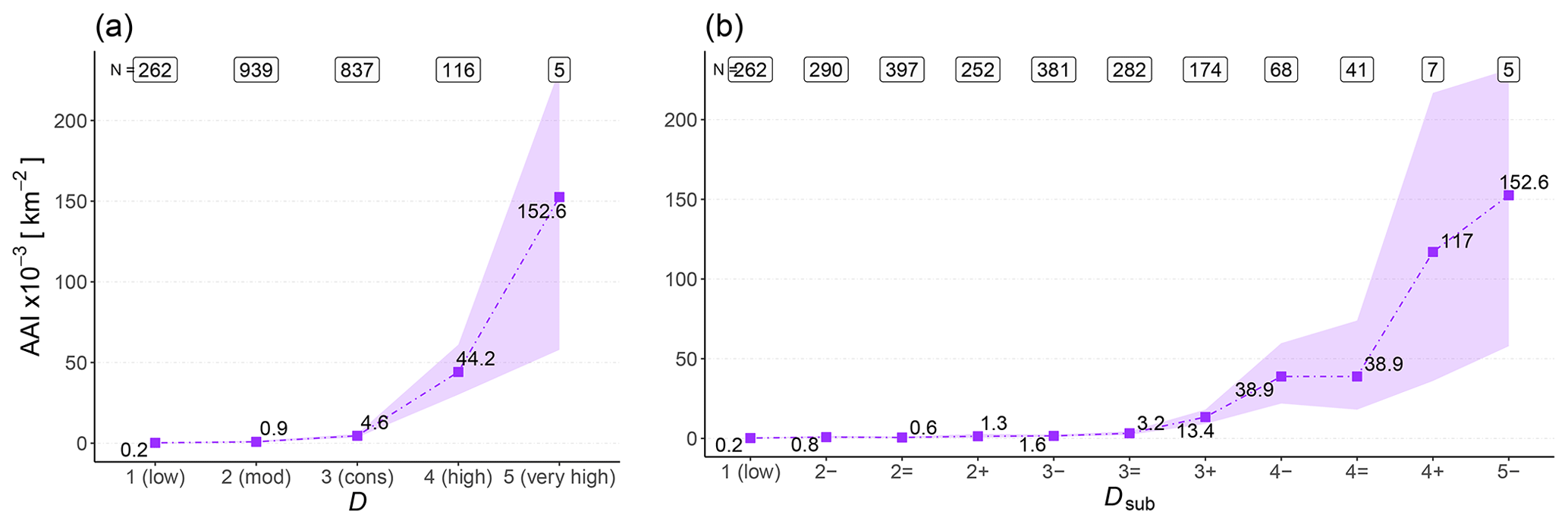
Figure 6 Avalanche activity index (AAI) for natural avalanches per 1000 km² potential release area (A_PRA) for (a) each danger level and (b) each sub-level. N represents the number of cases. Shown are the median values (points) and the 95% confidence interval (shaded area).

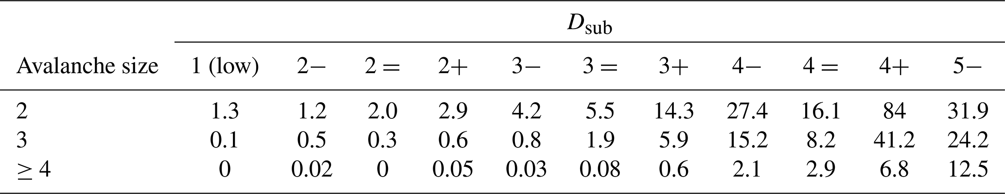
The increasing frequency of natural avalanche occurrence of increasing size with increasing danger level, as seen for the danger level D in Fig. 6a, is well reflected in D_sub (Fig. 6b). A significant positive correlation between D_sub and the avalanche activity index was found (r_s=0.35, p<0.001). Exceptions to this overall steady increase in $\stackrel{\mathrm{̃}}{\mathrm{AAI}}$ with increasing D_sub were found between 2⁻ and 2⁼ (F=0.7) and between 4⁻ and 4⁼ (F=1.0). Overall, $\stackrel{\mathrm{̃}}{\mathrm{AAI}}$ was rather low between 1 (low) and 3⁻ ($\stackrel{\mathrm{̃}}{\mathrm{AAI}}\le \mathrm{1.6}$) showing only a comparably small relative increase by a factor F=7.2 (Fig. 6b). For each danger level, an increase in $\stackrel{\mathrm{̃}}{\mathrm{AAI}}$ between the respective sub-level minus and plus was observed. This increase was lowest between 2⁻ and 2⁺ (F=1.7) and most pronounced between 3⁻ and 3⁺ (F=8.5). Even though $\stackrel{\mathrm{̃}}{\mathrm{AAI}}$ was higher at 5⁻ ($\stackrel{\mathrm{̃}}{\mathrm{AAI}}=\mathrm{152.6}$) compared to 4⁺ ($\stackrel{\mathrm{̃}}{\mathrm{AAI}}=\mathrm{117}$), this finding is based on a very small number of samples only (N=5 and N=7, respectively). The generally positive correlation between D_sub and avalanche activity was also visible when analyzing the number of avalanches of a certain size class: for instance, the number of avalanches of size ≥4 was very low at sub-level $\le {\mathrm{3}}^{=}$ (${\stackrel{\mathrm{̃}}{\mathit{\rho }}}_{\mathrm{nat},\mathrm{i}}\le \mathrm{0.08}$) but increased continuously with increasing danger level, peaking at 5⁻ (${\stackrel{\mathrm{̃}}{\mathit{\rho }}}_{\mathrm{nat},\mathrm{i}}=\mathrm{12.5}$). The number of natural avalanches of size 2 or size 3 showed the strongest increase between 2⁻ and 4⁻ (Table 3).

Table 2 Spatial density of natural avalanches ${\stackrel{\mathrm{̃}}{\mathit{\rho }}}_{\mathrm{nat},\mathrm{i}}$ (or number of avalanches) of size i per 1000 km² for each of the five danger levels D. Median values are shown.

Table 3 Spatial density of natural avalanches ${\stackrel{\mathrm{̃}}{\mathit{\rho }}}_{\mathrm{nat},\mathrm{i}}$ (or number of avalanches) of size i per 1000 km² for each of the sub-levels D_sub. Median values are shown.

5.2 Human-triggered avalanches and whumpfs

5.2.1 Human-triggered avalanches

The number of human-triggered avalanches per 10 000 km² (ρ_hum) increased significantly from 1 (low) to 2 (moderate) and from 2 (moderate) to 3 (considerable) (F≥4.2, p<0.001; Fig. 7a). At 4 (high), ${\stackrel{\mathrm{̃}}{\mathit{\rho }}}_{\mathrm{hum}}$ was lower compared to 3 (considerable). At least one human-triggered avalanche was reported on 3 % of the days in regions with a forecast of 1 (low) and on 50 % of the days when 3 (considerable) was forecast.

At the resolution of the forecast sub-levels, the number of human-triggered avalanches ${\stackrel{\mathrm{̃}}{\mathit{\rho }}}_{\mathrm{hum}}$ increased continuously from 1 (low) to 3⁺ (F≥1.2, Fig. 7b). At 4 (high), only about half as many human-triggered avalanches were reported compared to 3⁺. Human-triggered avalanches were observed more than 40 times more frequently at 3⁺ compared to 1 (low).

Human-triggered avalanches are comparably rare events. This means that ρ_hum,i is particularly sensitive to the size of the area as the likelihood that at least one human-triggered avalanche is reported increases with increasing potential avalanche terrain, given the same avalanche conditions. However, we were interested in true zeros (structural zeros) rather than sampling zeros (Ridout et al., 1998). For instance, sampling zeros may occur more often when the forecast refers to less terrain. Results obtained for approximately similar A_PRA for each danger level or sub-level showed a similar pattern, except that ${\stackrel{\mathrm{̃}}{\mathit{\rho }}}_{\mathrm{hum}}$ peaked at 3⁼. The corresponding Fig. A2 is shown in the Appendix.

5.2.2 Human-triggered whumpfs and shooting cracks

Observers seldom reported human-triggered danger signs at 1 (low) with less than 1 in 22 observations. In contrast, danger signs were rather common at 3 (considerable) and 4 (high) when ≥37 % of the observations indicated danger signs (Fig. 7c). These proportions increased significantly between all danger-level pairs (F>1.5, p<0.001). Furthermore, if danger signs were observed, an increasingly larger share was reported as frequent rather than rare with increasing danger level. For instance, 28 % of the observations, which indicated danger signs, were reported as frequent at 2 (moderate) but 54 % at 4 (high).

As can be seen in Fig. 7d, when considering D_sub, the proportions of observations mentioning danger signs increased in a strictly monotonic fashion with increasing D_sub (F>1.1; r_s=0.35, p<0.001). In addition, the proportion of reports indicating danger signs as frequent rather than rare increased from less than 30 % at $D_{\mathrm{sub}}\le {\mathrm{2}}^{+}$ to more than 50 % at 4 (high). This increase was monotonic between 2⁺ and 4 (high). In other words, with increasing sub-level, an increasing share of observations indicated at least one danger sign, while at the same time proportionally more danger signs were observed.

5.2.3 Accident–movement point ratio during backcountry touring

The accident–movement point ratio ($R_{\mathrm{acc}/\mathrm{move}}$) increased significantly from 1 (low) to 2 (moderate) (p<0.001) and from 2 (moderate) to 3 (considerable) (p<0.001), with a relative increase by a factor F of about 12 (Fig. 7e). The increase in ${\stackrel{\mathrm{̃}}{R}}_{\mathrm{acc}/\mathrm{move}}$ from 3 (considerable) (${\stackrel{\mathrm{̃}}{R}}_{\mathrm{acc}/\mathrm{move}}=\mathrm{1.2}\times {\mathrm{10}}^{-\mathrm{3}}$) to 4 (high) (${\stackrel{\mathrm{̃}}{R}}_{\mathrm{acc}/\mathrm{move}}=\mathrm{1.3}\times {\mathrm{10}}^{-\mathrm{3}}$) was not significant (p=0.33), which is also indicated by the large confidence interval at 4 (high) (CI = [0, $\mathrm{3.2}\times {\mathrm{10}}^{-\mathrm{3}}$]). ${\stackrel{\mathrm{̃}}{R}}_{\mathrm{acc}/\mathrm{move}}$ was significantly higher within the forecast core zone compared to fully outside the core zone.

As shown in Fig. 7f, ${\stackrel{\mathrm{̃}}{R}}_{\mathrm{acc}/\mathrm{move}}$ increased strictly monotonically with increasing D_sub from 1 (low) to 3⁺ (F>1.4). The total increase between 1 (low) (${\stackrel{\mathrm{̃}}{R}}_{\mathrm{acc}/\mathrm{move}}=\mathrm{0.074}\times {\mathrm{10}}^{-\mathrm{3}}$) and 3⁺ (${\stackrel{\mathrm{̃}}{R}}_{\mathrm{acc}/\mathrm{move}}=\mathrm{2.54}\times {\mathrm{10}}^{-\mathrm{3}}$) was by a factor 33. This increase was clearly visible also within 2 (moderate) (factor F 2.5 between 2⁻ and 2⁺) and 3 (considerable) (factor F 2.8 between 3⁻ and 3⁺). At 4 (high), the ratio was lower than at 3⁺, but this finding is based on very few data points (two accidents, 0.2 % of the movement points).

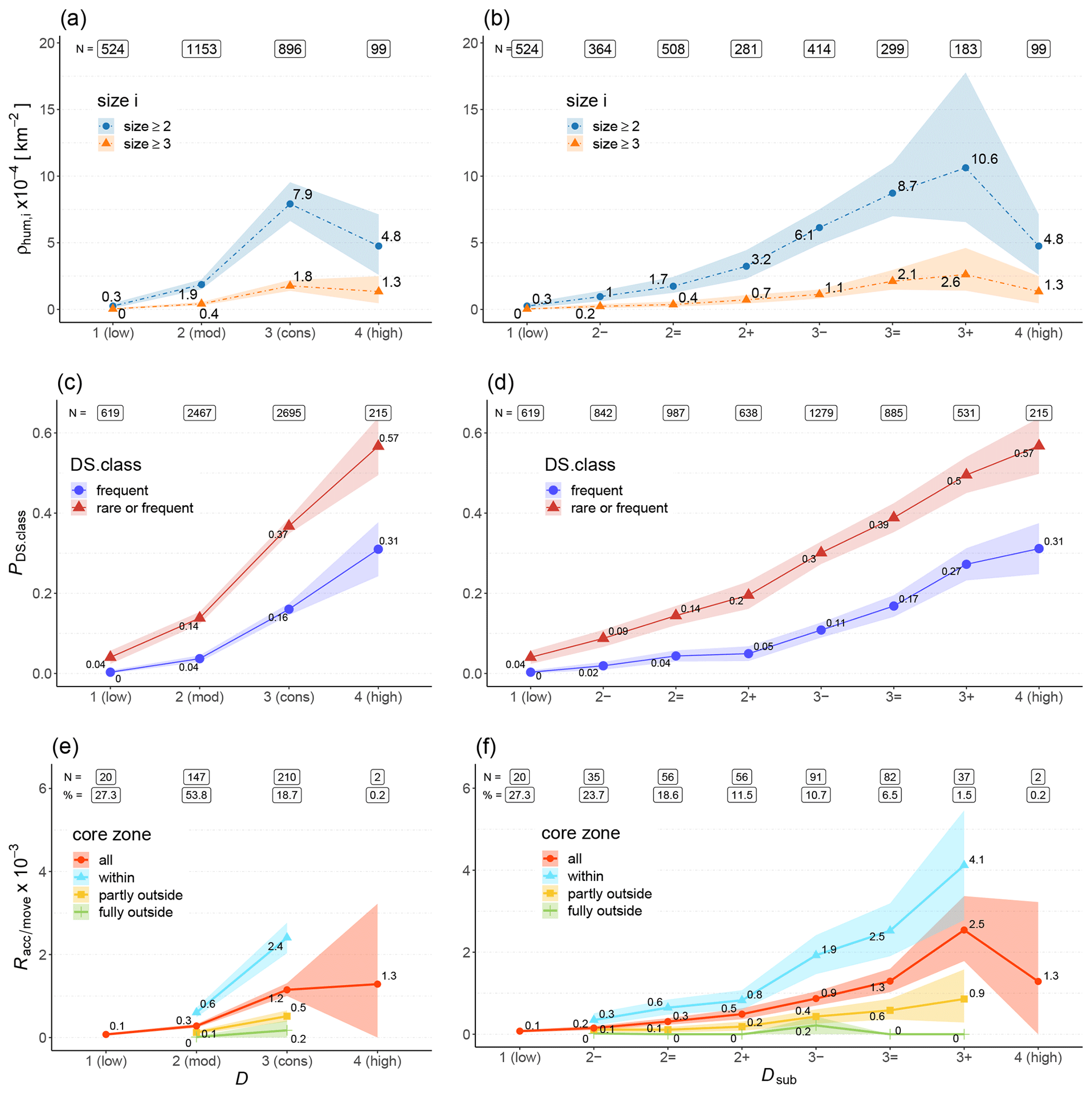
Figure 7 The density of human-triggered avalanches (or the number relative to the area of PRA) (ρ_hum,i) (a, b), the proportion of observations with reported danger signs (P_DS.class) (c, d), and the ratio of accident to movement points during backcountry touring ($R_{\mathrm{acc}/\mathrm{move}}$) (e, f) are compared to the danger level D (a, c, e) and sub-level D_sub (b, d, f). Shown are the median values (points) and the 95 % confidence interval (shaded area). N represents the number of danger regions (a, b), the number of observations (c, d), and the number of accident points (e, f). The number of movement points is expressed as percentage (%) relative to all movement points N=976 087.

In summary, a positive monotonic relationship between data related to the frequency of locations where human triggering is possible and D_sub exists within the range where a significant increase was noted for the conventional danger levels.

5.3 Stability tests

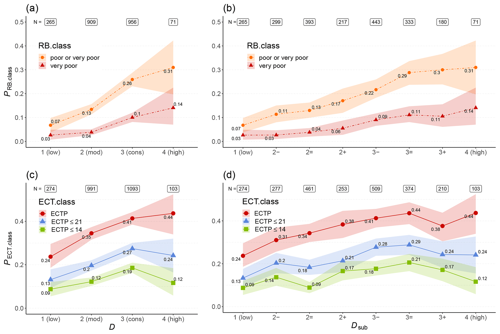
Figure 8 Proportion of Rutschblock test results (P_RB.class, a, b) and extended column test results (P_ECT.class, c, d) related to instability for tests observed at a specific danger level D (a, c) and sub-level D_sub (b, d). Shown are the median values (points) and the 95 % confidence interval (shaded area).

5.3.1 Rutschblock test

The median proportion of Rutschblock (RB) test results related to instability, ${\stackrel{\mathrm{̃}}{P}}_{\mathrm{RB}.\mathrm{class}}$, increased with increasing danger level D in a strictly monotonic fashion (F>1.2, Fig. 8a). Differences in P_RB.class between danger level pairs were significant for RB.class = very poor between 2 (moderate) and 3 (considerable) (p<0.001), as well as for the combined proportion of very poor and poor test results between 1 (low) and 2 (moderate) (p<0.001) and 2 (moderate) and 3 (considerable) (p<0.001).

Similar findings can be noted when analyzing the relationship between D_sub and P_RB.class (Fig. 8b): the combined proportion of very poor or poor RB test results increased continuously with increasing sub-levels (F≥1.04), with a weak but significant correlation (r_s=0.2, p<0.001). For RB.class = very poor this increase was strictly monotonic only between 2⁻ and 3⁼ (F≥1.2). Similarly, the correlation was weaker (r_s=0.12, p<0.001).

5.3.2 Extended column test

The median proportion of ECT results related to instability increased with increasing danger level from 1 (low) to 3 (considerable) (F>1.2, Fig. 8c). The difference in P_ECT.class values between subsequent danger levels was significant for ECTP and ECTP ≤ 21 from 1 (low) to 3 (considerable) (p≤0.02) and for ECTP ≤ 14 between 2 (moderate) and 3 (considerable). At 4 (high), P_ECT.class values were not significantly higher or were even lower than at 3 (considerable).

Analyzing the correlation between P_ECT.class and the sub-levels showed strictly increasing ${\stackrel{\mathrm{̃}}{P}}_{\mathrm{ECT}.\mathrm{class}}$ values with increasing D_sub between 1 (low) and 3⁼ for ECTP. No further increase was noted at higher D_sub. Similar patterns were observed for the proportion of ECTP ≤ 21 or ECTP ≤ 14, although the median value slightly decreased between 2⁻ and 2⁼. Again, the highest P_ECT.class values were found for 3⁼, with lower values at higher D_sub. The correlation between P_ECT.class and D_sub was generally weak though significant (r_s≥0.12, p<0.001).

In summary, we observed an increasing proportion of stability tests related to instability with increasing D_sub within the range in the danger scale where this increase was significant when comparing subsequent danger levels D. Similar to human-triggered avalanches (see Fig. 7a and b) or the accident–movement point ratio (see Fig. 7e and f), no further increase was noted at 3⁺ or 4 (high).

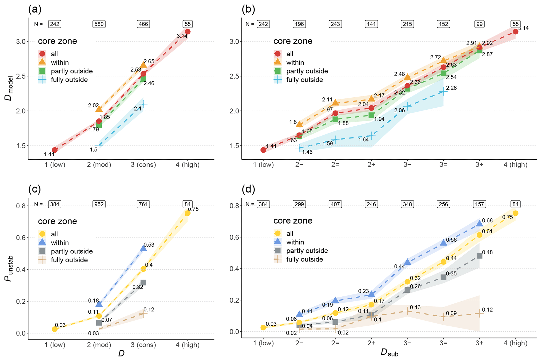
Figure 9 Output from random forest models predicting the danger level (a, b) and instability (c, d). The mean predicted danger level (D_model) and the proportion of simulated snow profiles predicted as unstable (P_unstab) are shown for all cases with the same danger level D (a, c) or sub-level D_sub (b, d). Shown are the median values (points) and the 95 % confidence interval (shaded area).

5.4 Models

5.4.1 Danger-level model

The danger rating predicted by the danger-level model showed a strong increase from 1 (low) (${\stackrel{\mathrm{̃}}{D}}_{\mathrm{model}}=\mathrm{1.44}$) to 4 (high) (${\stackrel{\mathrm{̃}}{D}}_{\mathrm{model}}=\mathrm{3.14}$; Fig. 9a). The increase was significant between all consecutive danger-level pairs (p<0.001). The absolute increase was on average 0.5 to 0.6 from one danger level to the next rather than a full level. Similar significant differences were found for predictions within the forecast core zone compared to those at locations and for aspects fully outside the core zone. The difference between these predictions was about 0.5 (p<0.001) and thus similar to the difference between neighboring danger levels.

Turning to D_sub, the same patterns can be noted (Fig. 9b): ${\stackrel{\mathrm{̃}}{D}}_{\mathrm{model}}$ increased continuously with increasing D_sub (F≥1.04). The correlation was strong and significant (r_s=0.79, p<0.001). The absolute increase from one sub-level to the next higher one was smallest from 2⁼ to 2⁺ (by 0.07), and for all other pairs the increase was ≥0.21. Furthermore, ${\stackrel{\mathrm{̃}}{D}}_{\mathrm{model}}$ was consistently higher within the core zone compared to fully outside the core zone.

5.4.2 Instability model

The median proportion of simulated profiles classified as unstable (${\stackrel{\mathrm{̃}}{P}}_{\mathrm{unstab}}$) increased with increasing danger level from 0.03 at 1 (low) to 0.75 at 4 (high). The increase was significant between all consecutive danger-level pairs (p<0.001). As shown in Fig. 9c, ${\stackrel{\mathrm{̃}}{P}}_{\mathrm{unstab}}$ was considerably higher within the forecast core zone than fully outside (p<0.001).

Findings were similar when exploring the correlation between P_unstab and D_sub (Fig. 9d): ${\stackrel{\mathrm{̃}}{P}}_{\mathrm{unstab}}$ increased monotonically with increasing D_sub showing a strong, positive correlation (r_s=0.76, p<0.001). In addition, values within the core zone were always higher than outside the core zone. It is further noteworthy that ${\stackrel{\mathrm{̃}}{P}}_{\mathrm{unstab}}$ values were similarly low outside the core zone for all sub-levels within 3 (considerable) (${\stackrel{\mathrm{̃}}{P}}_{\mathrm{unstab}}\le \mathrm{0.13}$).

6 Discussion

The overarching research question we explored was as follows: given the daily observations and measurements, often still incomplete at the time when avalanche forecasters in Switzerland meet for their afternoon forecaster briefing, and a numerical weather prediction model, can human avalanche forecasters forecast avalanche hazard for the following day with higher resolution than the five danger levels? To this end, we analyzed a wide variety of data related to the contributing factors of avalanche hazard and investigated their relationship with sub-levels assigned to danger levels in Switzerland. The specific question we had was therefore, given the current forecasting set-up in Switzerland, whether the sub-levels were assigned in a way that they express the expected rank-order relationship between the three contributing factors of avalanche hazard and the sub-levels. As we could not rely on a clear definition of the sub-levels, we split the analysis into two steps: first, we determined the range of the danger scale in which a given data source was valuable to distinguish between danger levels. Second, we analyzed whether a monotonic correlation between sub-levels and the data source existed.

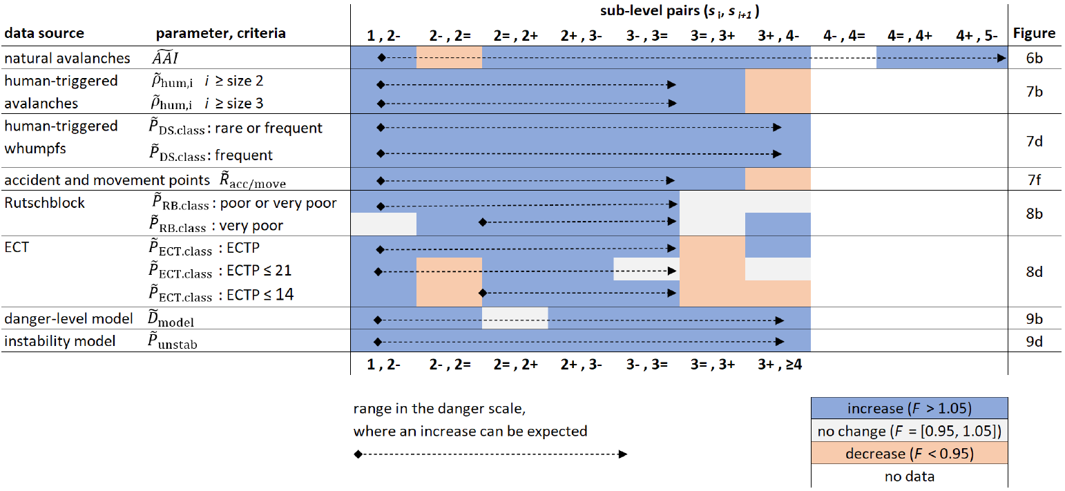
For the first research question, we determined in which range of the danger scale a data source was suitable for our analysis. As summarized in Table 4 by the arrows, natural avalanches, human-triggered whumpfs, and the two models were the most suitable, allowing the analysis of the entire range of the danger scale for natural avalanches and from 1 (low) to 4 (high) for the other three data sources. In contrast, and except for the human-triggered whumpfs, data that require a human being present in avalanche terrain were most suitable at danger levels 1 (low) to 3 (considerable). Of limited use were the two stability tests and here particularly the stability classes with the most restrictive class thresholds ($P_{\mathrm{RB}.\mathrm{class}}=$ very poor, $P_{\mathrm{ECT}.\mathrm{class}}=$ ECTP ≤ 14). This first step was not only an important foundation for the second part of our analysis, but it also confirmed that – on average – the forecast danger levels have the intended predictive value concerning the three contributing factors of avalanche hazard.

Turning to our second research question, we summarize an increase in the value of the analyzed parameters for most of the sub-level pairs (s_i, s_i+1) within the range where this could be expected if the relative assignment of the sub-levels was consistent on average and if the data permitted this. Of the 74 sub-level pair comparisons shown in Table 4, 69 showed an increase from s_i to s_i+1 with F≥1.05 (light blue cells) and only two a decrease with F≤0.95 (light orange cells).

These findings represent the average. Of course, there will be errors in both the forecast danger level (absolute judgment) and the forecast sub-level (comparative judgment). For instance, a recent study explored the agreement between danger-level assessments provided by specifically trained observers after a day in the field (local nowcasts) and the forecast regional danger level (Techel et al., 2020b). This study showed a difference in danger level between the forecast danger level and the danger level determined by the observers 19 % of the time for cases when two observers in the same small warning region unanimously indicated the same danger level. However, in these cases, the difference between the local nowcasts of avalanche danger and the forecast danger level and sub-level was often less than a full danger level: most often (70 %), the sub-level qualifier was the one closest to the local estimates. Thus, assigning a sub-level can provide an important indication of the severity within a danger level and therefore has the potential to reduce the magnitude of the forecast error. A useful example to illustrate this is the comparison of natural avalanche activity between neighboring sub-levels belonging to two danger levels, as, for instance, 4⁺ and 5⁻. The avalanche activity was more similar at these two sub-levels ($\stackrel{\mathrm{̃}}{AAI}=\mathrm{117}$ and $\stackrel{\mathrm{̃}}{AAI}=\mathrm{153}$, respectively, Fig. 6b) than when comparing 4 (high) ($\stackrel{\mathrm{̃}}{\mathrm{AAI}}=\mathrm{44}$) with 5 (very high) ($\stackrel{\mathrm{̃}}{\mathrm{AAI}}=\mathrm{153}$, Fig. 6a).

Table 4 Table summarizing whether an increase (light blue, F>1.05) or a decrease (light orange, F<0.95) in the median was observed from one sub-level (s_i) to the next higher one (s_i+1). The dashed arrows indicate the range, for which significant increases between neighboring danger-level pairs (D, D+1) were observed, and where, thus, an increase between sub-levels can be expected if their relative assignment would on average be correct.

6.1 Implications for forecasters

Forecasters felt generally comfortable assigning a sub-level in dry-snow conditions. We attribute this to the fact that forecasters must characterize the severity of the avalanche conditions to accurately describe the situation in the forecast, regardless of whether a sub-level is assigned or not. However, assigning a sub-level makes this evaluation more systematic and facilitates communication with other forecasters on duty. Forecaster feedback suggests that the additional mental effort required for the assignment of a sub-level is small and that discussing the sub-level at the forecaster briefing does not take more time than discussing any of the other elements which are communicated in the forecast products.

Our analysis showed that forecasters can estimate sub-levels in dry-snow conditions based on the available data, thus providing a way of increasing the resolution of the forecast danger level while maintaining the well-established standard of assessing and communicating avalanche hazard using the five danger levels. Moreover, the comparison with the two models not used in the forecast production process indicated that the sub-level forecasts were reasonably consistent. The models mirrored differences in the forecast danger level and the sub-level, as well as concerning aspects and elevations where the danger prevailed.

Refined danger ratings allow forecasters to express a more natural and gradual change in avalanche danger compared to the five danger levels. While models have the potential to provide continuous output, such an approach is not possible for humans. Therefore, the experts assessed avalanche danger in two stages combining an absolute and a relative judgment (Kahneman et al., 2021): first, forecasters determined the danger level before they performed a comparative sorting within this level. The definition of the danger levels provides the absolute anchor, while the forecasters' experience concerning the variation within a danger level is relevant for the comparative judgment. Based on our findings, we conclude that the specification of a sub-level is possible using such a procedure, regardless of whether an avalanche warning service relies on measurements, observations, and a weather forecast or whether the forecast production relies more strongly on numerical models. However, prerequisites to refine sub-levels are that enough data relevant to the forecasting task are sufficiently available in time and space and that the assessment is made using a sufficiently detailed spatial and temporal resolution (Techel et al., 2020b). In conventional avalanche hazard assessment, increasing the resolution of the avalanche forecast is limited by the data available at the time of the assessment and the available resources of the avalanche forecasters. With the use of models, the resolution can be increased, and at the same time the noise, i.e., the random errors, can be reduced. Thus, in the future, such models could become a viable addition to assess and forecast avalanche danger at a regional level, complementary to the more conventional way of forecasting, permitting a greater spatial and temporal resolution of the forecast.

While we have shown that the method of combining absolute and relative judgments can result in avalanche danger assessments with finer granularity, it might still be advantageous to describe typical characteristics for each sub-level. This may not only help forecasters when deciding on a sub-level but may potentially also be useful for users of this information. Therefore, we envision that by using the presented data, but also the actual descriptions of avalanche danger in the avalanche forecast (Hutter et al., 2021), a data-driven description of the sub-levels could be obtained.

6.2 Practical applications

We have demonstrated that, on average, the forecast sub-levels have predictive value; that is, they correlate with the three contributing factors of avalanche hazard. Therefore, we argue that the sub-levels should be provided in a suitable form to forecast users as they may support the decision-making process.

We see two potential use cases. The first, more traditional use case is the provision of the sub-levels as part of the avalanche forecast product, permitting a direct interpretation of the sub-level by the human forecast user. However, as several studies have shown, the comprehension of the information communicated in the bulletin is strongly related to the education of the user and to the complexity of the avalanche situation (e.g., Engeset et al., 2018; St. Clair et al., 2021). Therefore, we consider it important that the provision of this information to the public does not violate the structure of the information pyramid. This can be taken into account by retaining the defined danger levels and their (optional) subdivision (sub-level). Questions that arise are, for instance, for which user group this additional information should be available and how it should be presented so as not to reduce the comprehensibility of the forecast. Another option would be to pass on this information to the public indirectly by feeding it primarily into algorithms which build upon the avalanche forecast, such as a classification of avalanche risk for ski tours as on the website https://www.skitourenguru.ch// (last access: 7 June 2022) (Schmudlach, 2022). When used by such algorithms, sub-levels can increase the precision of the forecast without causing problems with comprehensibility.

Second, the sub-levels could also be used for the development and validation of models. These may, in turn, improve avalanche forecasting. One such example is the danger-level model, which was trained and validated with the defined danger levels (Pérez-Guillén et al., 2021). The danger-level model already captured differences in avalanche danger between the sub-levels and the core zone. However, we surmise that re-training the model incorporating the information contained in the sub-level may potentially increase the model performance further.

6.3 Limitations

We aimed at exploring the correlation between D_sub and data related to the contributing factors of avalanche hazard. However, the results are not only influenced by the quality of D_sub but also by potential errors in the assignment of a danger level D, which is the first step in the assessment process, or in the spatial clustering of warning regions to regions with the same conditions (i.e., danger regions shown in Fig. 2a). In addition to errors related to the forecast, errors and bias may also be present in the data used in this analysis. Of particular relevance are non-random errors or bias, for instance, due to sampling or reporting preferences or due to human behavior as a consequence of avalanche conditions. As we cannot decompose the analysis into these various error sources, we are unable to quantify them. However, assuming that non-random errors or the magnitude of bias in the data do not change abruptly between consecutive sub-levels, we argue that overall trends should be captured.

Our study was set in Switzerland. While the results can therefore not readily be applied to other countries, we believe that the more general finding, namely the approach of combining absolute and relative judgments, should be applicable in other forecast settings as well.

The distribution of the data was not uniform over the entire forecast domain. For instance, hardly any data were available for the Jura or middle and southern Ticino regions (region B in Fig. 2a). Thus, it is unclear whether the assignment of the sub-levels is of equal quality in these areas. Furthermore, for the higher danger levels and sub-levels (4 (high) and 5 (very high)), the data sets are comparably small.

7 Conclusions

Can forecasts of avalanche danger be refined by using a combination of absolute and comparative judgments? We addressed this question by comparing 5 years of Swiss avalanche forecasts including a sub-level qualifier (comparative judgment) assigned to the danger level (absolute judgment) with several data sources considered a proxy for the three contributing factors of avalanche hazard. We have shown that, on average, these sub-levels reflect the expected increase in the number of locations with poor snowpack stability and in the number and size of avalanches with increasing forecast sub-level.

Our findings are specific to the current forecast set-up in Switzerland. However, we surmise that avalanche warning services whose hazard assessment is based on a similar temporal and spatial scale as is used in Switzerland should also be able to refine their assessments if (1) enough relevant data in time and space are available and (2) a similar approach combining absolute and relative judgments is used. We like to emphasize that warning services, which intend to assign sub-levels to a danger level, should make an effort to explore their quality, particularly if their communication in forecast products is envisioned. Such quality assessments, however, should not only be made for sub-levels but for any information conveyed in forecast products.

The sub-levels clearly increase the predictive value of the forecast, opening the discussion on how this information could be provided to forecast users.

Appendix A

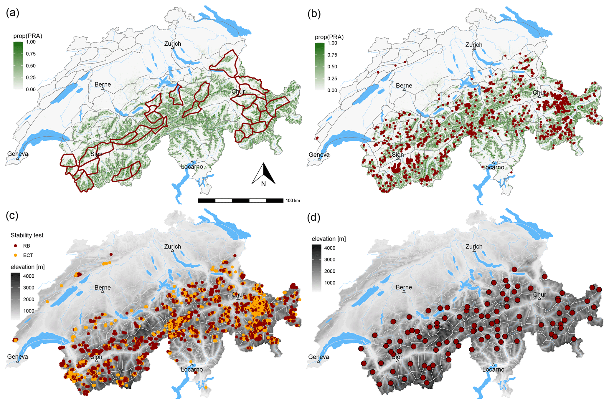
Figure A1 Maps of Switzerland showing (a) the warning regions (grey polygon boundaries) and those selected for the analysis of natural avalanches (bold polygons), (b) the location of human-triggered avalanches (dots), (c) the location of stability tests (dots), and (d) the location of the automatic weather stations where the two models were run (points). For illustration purposes, color shading in the background represents (a, b) the proportion of potential release areas (prop(PRA)) according to Bühler et al. (2018) per 500×500 m grid cells and (c, d) elevation based on a digital elevation model (source: SwissTopo).

Figure A2 The density of human-triggered avalanches (or the number relative to the surface area) compared to (a) the danger level D and (b) the sub-level D_sub. Shown are the median values (points) and the 95 % confidence interval (shaded area). N represents the number of danger regions. Here, we restricted the analysis to cases when the same D_sub was forecast for regions with approximately similar A_PRA. The resulting median A_PRA was between 2000 and 2300 km² for each D_sub.