the Creative Commons Attribution 4.0 License.
the Creative Commons Attribution 4.0 License.
 | 19 May 2022
The role of heat wave events in the occurrence and persistence of thermal stratification in the southern North Sea
Joanna Staneva
Sebastian Grayek
Johannes Schulz-Stellenfleth
Jens Greinert
Temperature extremes not only directly affect the marine environment and ecosystems but also indirectly influence hydrodynamics and marine life. In this study, the role of heat wave events in the occurrence and persistence of thermal stratification was analysed by simulating the water temperature of the North Sea from 2011 to 2018 using a fully coupled hydrodynamic and wave model within the framework of the Geesthacht Coupled cOAstal model SysTem (GCOAST). The model results were assessed against reprocessed satellite data and in situ observations from field campaigns and fixed Marine Environmental Monitoring Network (MARNET) stations. To quantify the degree of stratification, the potential energy anomaly throughout the water column was calculated. The air temperatures and potential energy anomalies in the North Sea (excluding the Norwegian Trench and the area south of 54∘ N) were linearly correlated. Different from the northern North Sea, where the water column is stratified in the warm season each year, the southern North Sea is seasonally stratified in years when a heat wave occurs. The influences of heat waves on the occurrence of summer stratification in the southern North Sea are mainly in the form of two aspects, i.e. a rapid rise in sea surface temperature at the early stage of the heat wave period and a higher water temperature during summer than the multiyear mean. Another factor that enhances the thermal stratification in summer is the memory of the water column to cold spells earlier in the year. Differences between the seasonally stratified northern North Sea and the heat wave-induced stratified southern North Sea were ultimately attributed to changes in water depth.
- Article
(9133 KB) - Full-text XML
-
Supplement
(17515 KB) - BibTeX
- EndNote


In recent decades, extreme temperature events have increased in frequency with global climate change, and these events have attracted growing attention from both regional and global research on earth systems (IPCC, 2022; Herring et al., 2015). Summer heat waves are frequently occurring extreme meteorological events (Perkins and Alexander, 2013) that anomalously warm seawater in discrete periods via local air-sea heat fluxes; these periods are known as marine heat waves (MHWs) (Pearce et al., 2011; Hobday et al., 2016). Other causes of MHWs include ocean heat transport (Rouault et al., 2007; Oliver et al., 2017) and remote forcings (Bond et al., 2015; Hu et al., 2017). An increasing intensification trend of MHWs has recently been identified (Oliver et al., 2020). In this context,over the last two decades, numerous record-breaking MHW events have been reported in the Mediterranean Sea (Bensoussan et al., 2010), the Tasman Sea (Oliver et al., 2017; Perkins-Kirkpatrick et al., 2019), West Australia (Feng et al., 2013), the Northeast Pacific (Hu et al., 2017), the western South Atlantic (Manta et al., 2018) and the East China Sea (Tan and Cai, 2018). Accordingly, due to the substantial influences of MHW events on marine hydrodynamics and ecosystems, the field of research on MHWs has rapidly grown (Wernberg et al., 2013, 2016; Oliver et al., 2020).
The North Sea, which is located on the passive continental margin of northwest Europe, connects the Baltic Sea in the east to the Atlantic through the Norwegian Sea in the north and the English Channel in the west (Fig. 1). The water depths in most areas of the North Sea are shallow, except for the Norwegian channel, which has an average depth of 400 m with a maximum depth of 750 m in the Skagerrak (Otto et al., 1990). The tidal circulation is dominated by the semidiurnal (M2 and S2) tides and interacts with the North Sea bathymetry. Due to these relatively shallow water depths, the sources of turbulent mixing are tidal currents at the bottom (Hill et al., 1994) and wind-induced waves at the water surface (Staneva et al., 2017). The North Sea, which is strongly impacted by extreme meteorological events, has been predicted to be warming twice as fast as the global levels (Smale et al., 2019; Hobday and Pecl, 2014); nevertheless, the consequences of MHWs, have received little attention (Wakelin et al., 2021).
During the summer of 2018, extreme heat wave events with record-breaking temperatures were observed in many countries. The German Weather Service (Deutscher Wetterdienst, DWD) observed weekly temperature anomalies of up to +3–6 ∘C (Imbery et al., 2018). In addition to west and north Europe, which suffered significant social and environmental impacts, the North Sea (specifically, the natural processes therein) was heavily perturbed by these summer heat waves. For example, Borges et al. (2019) found that the dissolved methane concentration in surface waters along the Belgian coast was three times higher during the summer of 2018 than during a normal year. Hence, the heat wave events that struck Europe in 2018 provide a good opportunity to investigate the impacts of extreme meteorological conditions on the development of density stratification in the southern North Sea. In particular, extreme temperature events were identified in the recently published Ocean State Report 5, which also documented how these events may impact key fish and shellfish stocks (Wakelin et al., 2021); however, to the best of our knowledge no systematic investigation has been performed to explain these impacts in relation to the changes in vertical stratification during extreme temperature events in the North Sea.
In the North Sea, the development of vertical thermal stratification, a fundamental physical process, is associated with the seasonal cycling of water temperatures, especially on the shallow shelf. From early May to late September, the majority of the North Sea becomes stratified, which is also known as the summer stratification (Pingree and Griffiths, 1978). Understanding the occurrence of this summer stratification and its temporal and spatial variations is important and thus has been the focus of many studies (Becker, 1981; Elliott and Clarke, 1991; Pohlmann, 1996; Schrum et al., 2003; Stips et al., 2004; Sharples et al., 2006; van Leeuwen et al., 2015). On the shallow shelf, stratification plays an essential role in, e.g. water circulation (van Haren, 2000; Luyten et al., 2003), sediment flocculation and transport (Fettweis et al., 2014), phytoplankton growth (Nielsen et al., 1993; Fernand et al., 2013) and fishery management (Sas et al., 2019).
Many relevant modelling studies have been conducted within the North Sea (Luyten et al., 2003; Stips et al., 2004; Sharples et al., 2006; Mathis et al., 2015). Klonaris et al. (2021) recently developed a state of the art three-dimensional hydrodynamic model based on the Regional Ocean Modeling System (ROMS) and accurately reproduced the thermohaline variations in the southern North Sea. Other models have been employed to investigate thermodynamic air-ocean interface processes by coupling the interactions between the air and sea systems (Ho-Hagemann et al., 2017; Stathopoulos et al., 2020). For instance, Staneva et al. (2021) presented a new high-resolution model (part of the Geesthacht Coupled cOAstal model SysTem, GCOAST) that couples ocean and wave model systems for the North Sea and the Baltic Sea; this model implements parameterizations that take the nonlinear feedback between tidal currents and wind waves into account. Within this framework, Chen et al. (2021) developed a three-dimensional variational (3DVAR) data assimilation scheme that improved the modelling of sea surface temperature in the North Sea; the authors further quantified the impact of temperature assimilation on the heat budget estimates for the North Sea.
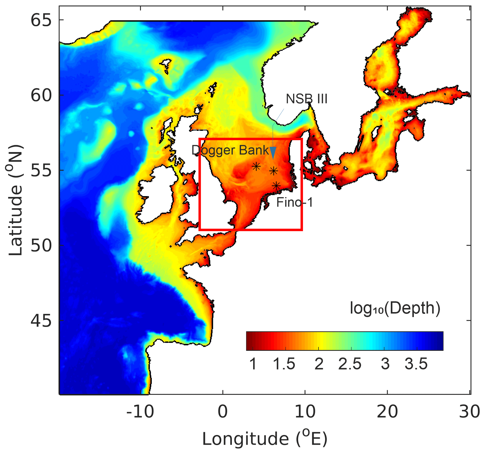
Figure 1GCOAST model domain. The bathymetry (m) is shown on a logarithmic scale. The locations of the observations from the Poseidon cruise (Dogger Bank) and MARNET stations (NSB III and Fino-1) are indicated with asterisks. The red frame defines the area of the middle and southern North Sea.
Based on 51 years of simulation data, van Leeuwen et al. (2015) identified five regimes in the North Sea regarding different types of density stratification. They classified the presence of stratification according to the influence of freshwater from estuaries, permanent haline stratification in the deep Norwegian Trench, seasonal changes in air temperatures, and strong turbulent mixing by tidal currents and waves; however, their categories failed to include approximately 30 % of the North Sea area, especially its southern part, where the water depth is generally less than 50 m and approximately half of the total area lacks a dominant stratification regime. The density stratification in this area is particularly sensitive to changes in climate and exhibits interannual variations. Therefore, the present study focuses on this unclassified area to quantify the role of heat waves in the occurrence of summer stratification. We further seek to identify the main factors that affect the intensity and duration of the thermal stratification in the southern North Sea.
This study applied a fully coupled hydrodynamic and wind-wave model to the North Sea and the adjacent sea areas. The model simulation results were compared with both short-term (a cruise campaign from 23 July to 1 August 2018) and multiyear (6-year stationary measurements) acquired in recent years. Furthermore, 38 years of sea surface temperature (SST) data were reprocessed from satellite observations to detect the occurrence and duration of MHWs. The details of the observations and the methods used for analysis are described in the next section. The results are presented in Sect. 3, and the discussion follows in Sect. 4. The main conclusions are given in Sect. 5.
2.1 Model
This study conducted an 8-year (2011–2018) numerical simulation with the Nucleus for European Modelling of the Ocean (NEMO) ocean circulation model (Madec and the NEMO team, 2016) fully coupled to the wave model WAM (The Wamdi Group, 1988; Günther et al., 1992). This model allowed us to analyse the extreme year of 2018, which is a focus of our research as well as several past heat wave events and cold spells. The model was implemented under the GCOAST framework covering the Northwest European Shelf, the North Sea, and the Baltic Sea, and it has a horizontal resolution of approximately 3.5 km with the vertical resolution of the NEMO standard hybrid grid with 50 levels. The present study focuses on the southern North Sea, which is defined as the area within −3–9∘ E longitude and 51–57∘ N latitude (red frame in Fig. 1).
For the boundary conditions, the temperature, salinity and barotropic forcing were derived from the hourly output of the Copernicus Marine Environment Monitoring Service (CMEMS) Forecast Ocean Assimilation Model (FOAM) Atlantic Margin Model version 7 (AMM7) (O’Dea et al., 2012). Tidal harmonic constituents derived from the TPXOv8 model were applied at the open boundaries to force the tidal motions (Egbert and Erofeeva., 2002). The data from the European Centre for Medium-Range Weather Forecasts (ECMWF) Reanalysis version 5 (ERA5) were used at the water surface (Hersbach et al., 2020). The ERA5 data included the air temperature 2 m above the water surface, which was also applied to analyse the relation between the variation in air temperature and the thermal stratification in the North Sea. The model adopted a baroclinic time step of 100 s. Turbulent eddy viscosities/diffusivities were computed with a “k−ϵ” turbulence closure scheme with the generic length scale (Umlauf and Burchard, 2003). Further details of the model are documented in Chen et al. (2021).
2.2 Observation data
In situ data were acquired by two different methods. From 23 July to 1 August 2018, field measurements were conducted in the Dogger Bank (Fig. 1) during Poseidon cruise POS526. This was part of a multidisciplinary research initiative of the GEOMAR Helmholtz Center for Ocean Research (GEOMAR, 2019). During the cruise, high-resolution temperature and salinity data were sampled by conductivity-temperature-depth (CTD, Sea-Bird SBE 49 FastCAT) measurements. Long-term (interannual) data were further obtained from two fixed automatic oceanographic platforms in the North Sea: Nordseeboje III (NSB III, N and E) and Fino-1 ( N and E)(see Fig. 1). Both platforms are part of the Marine Environmental Monitoring Network (MARNET), which is operated by the German Federal Maritime and Hydrographic Agency (Bundesamt für Seeschifffahrt und Hydrographie, BSH). On these MARNET platforms, water temperature and salinity at different depths are collected continuously and processed to an hourly interval.
A time series of SST data spanning 38 years (1982–2019) was derived from the European Space Agency (ESA) SST Climate Change Initiative (CCI) Level 3 (1982–2016) (Merchant et al., 2019) and the Copernicus Climate Change Service (C3S) Level 3 product (2016–2019). These daily mean datasets cover the Northwest European Shelf with a spatial resolution of . The data were retrieved from the Copernicus Marine Service (https://resources.marine.copernicus.eu/, last access: 3 May 2022).
2.3 Temperature analysis
Each calendar year was divided into two separate seasons, i.e. the cold season and the warm season, according to the interannual trend of air temperatures. Normally, the cold season lasts from September to mid-April of the following year, while the warm season endures from mid-April to August. In the cold season, cold spells are considered to occur when there are at least 5 consecutive days in which the temperature is lower than the threshold of the 10th percentile (Wakelin et al., 2021). In the warm season, MHW events are identified, following the criteria introduced by Hobday et al. (2016), i.e. when the water temperature exceeds the threshold of the 90th percentile within in a period of at least 5 consecutive days.
2.4 Quantification of stratification
As introduced by Simpson (1981), the potential energy anomaly ϕ, is frequently used as a suitable measure of the degree of stratification. This variable indicates the amount of mechanical energy (per m3) required to instantaneously homogenize the water column with a given density stratification. The parameter ϕ is defined as follows:
where
is the vertical mean water density and is the gravitational constant of acceleration. The instantaneous total water depth is given by , where η and H are the sea surface elevation and time-average water depth, respectively. Note that the water density ρ, which is not part of the standard NEMO model output, was calculated (at 1 atm) following Millero and Poisso (1981) (details are provided in Appendix A).
To quantify the vertical stratification and evaluate its suitability, the gradient Richardson number, Ri, is computed:
with the definition of the buoyancy frequency
and the vertical shear
Here, u and v are the horizontal velocity components (m s−1) obtained from the model in the same time interval as those of the temperature and salinity data.
The simulation results were compared with the in situ measurements obtained by the Poseidon cruise and oceanographic platforms (Fig. 2). The model was capable of capturing the main observed features. At MARNET station NSB III, which is located in the central eastern part of the southern North Sea (see Fig. 1), the temporal variations in the simulated air temperature followed the seasonal cycles of the observed air temperature from 2011 to 2018. The observed and simulated water temperatures usually diverged during the warm season of each year (May–September). The interannual cycle of the water temperature followed the interannual variation in the air temperature above the sea surface; however, the intensity of the water stratification showed no obvious seasonal pattern; instead, the thermal stratification was more related to air temperature changes. For example, large stratification occurred during the summers of 2014 and 2018, when the surface–bottom temperature difference was much larger than that during the periods before and after (the surface–bottom temperature difference was not apparent during 2015 and 2017, and the fluctuations in the air temperature were small). The differences between the modelled and measured water temperatures were in the range of ±2 ∘C, and the model error was smaller during the winter months than in the summer months.
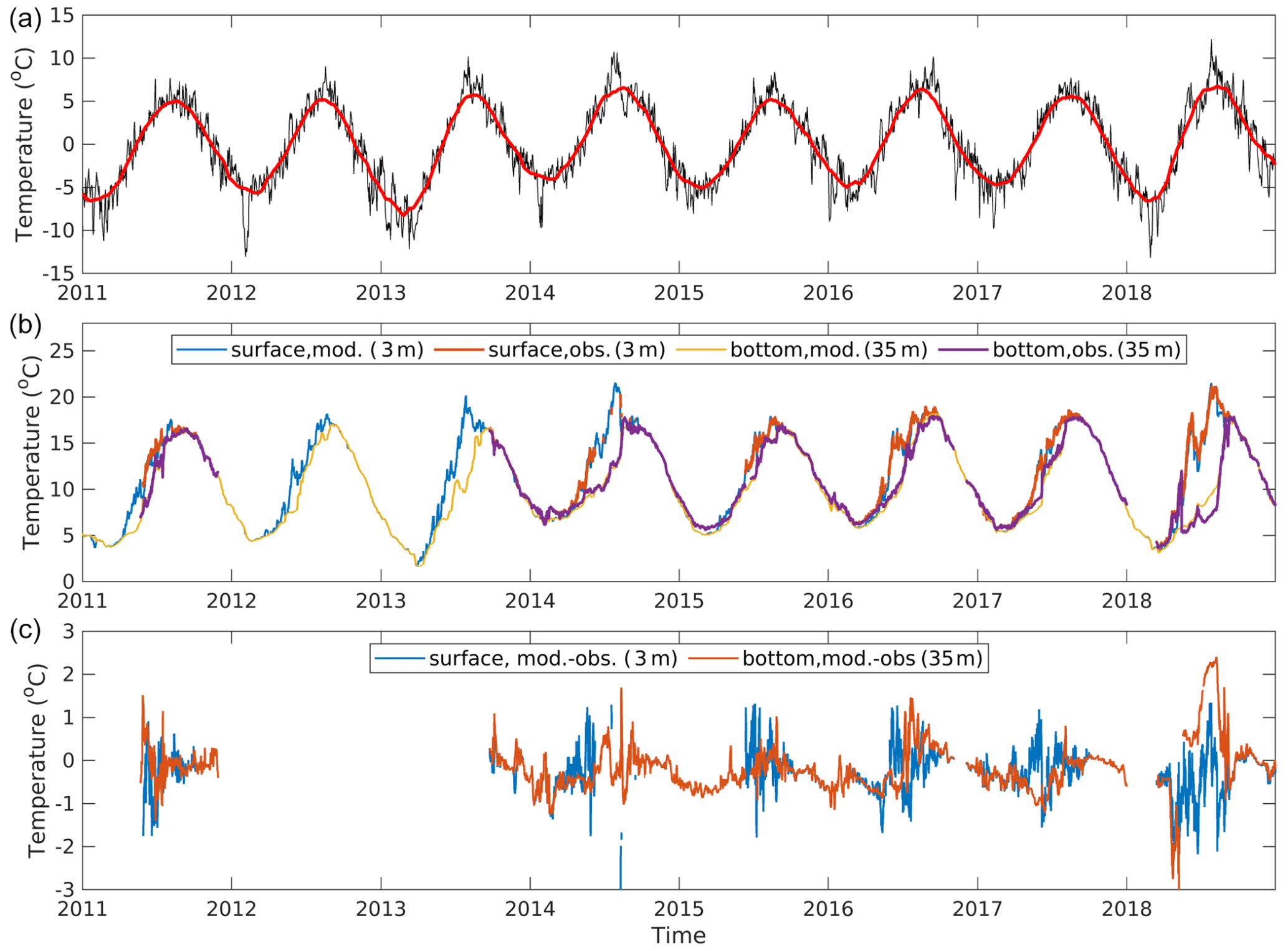
Figure 2(a) Interannual variation in the air temperature (with the multiyear mean removed) at NSB III. The black line is the daily air temperature, and the thick red line represents the 3-month moving average. (b) The interannual variation in the observed (obs.) and simulated (mod.) water temperatures at the surface and the bottom of the same location. (c) Water temperature differences between the model and the in situ measurements at the surface and the bottom.
Figure 3 further compares the simulated data and observations at different locations in the southern North Sea in July 2018. In the Dogger Bank and at the NSB III site, the model reproduced high temperatures within a thin layer (approximately 5–10 m) near the surface. The water temperature exhibited temporal variation mainly in the upper water layers (above 20 m depth). Below 20 m, the water temperature was relatively stable at approximately 10 ∘C. The differences between the surface and the bottom reached more than 15 ∘C in both the model and the observations. At Fino-1, there was almost no difference between the modelled water temperature and the in situ measurements; however, inconsistencies were observed between the simulated data and observations. The model overestimated the observations in the deeper layers. For instance, below 20 m, the model yielded temperatures approximately 1–3 ∘C higher than the in situ data in the Dogger Bank and at site NSB III.
In general, the fully coupled model is capable of reproducing the characteristics of the water temperatures in the North Sea. The model errors were small compared to the annual water temperature variations. One reason for the discrepancies between the model and observations is that the spatial and temporal resolutions of the atmospheric forcing data are coarse. In July–August 2018, the modelled bottom water temperature was warmer than observed (Fig. 2). During this heat wave period, a strong spatial temperature gradient was observed, which led to additional heat transport from shallower to deeper regions. At the NSB III site, the observed density stratification in the water column was underestimated by the model; however, considering that the model error is much smaller than the surface-bottom temperature differences (10–12 ∘C), the main conclusions of the present study are unaffected.
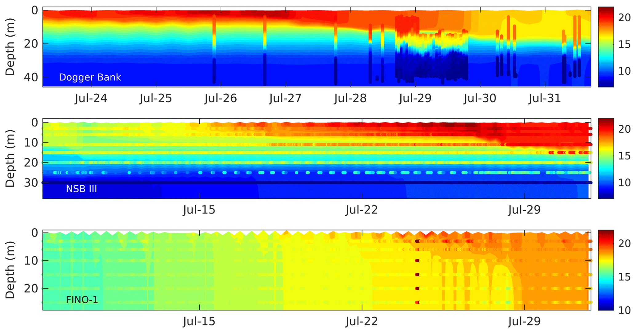
Figure 3In situ measured and model simulated water temperatures (in ∘C) in July. In the Dogger Bank (upper panel), measurements were obtained by a CTD profiler during the Poseidon campaign. At the MARNET stations NSB III (middle panel) and Fino-1 (lower panel), temperatures were measured in fixed water layers.
The results were further compared with reprocessed satellite data. Figure 4 shows the annual variations in the modelled and remotely sensed SST at the NSB III platform in 2018. The features of the annual SST variations at other stations were similar to those at NSB III and thus are not shown. The model reproduced the satellite data from January to May and from mid-August to December with errors of less than 1 ∘C. Differences between the two datasets were mainly found from June to August, when the fluctuations in the reprocessed satellite data were much smaller than those in the model. This could be attributed to the smoothing of the measurements by the gridding and gap-filling of level 3 data. The MHWs in the North Sea region were detected with the 90th percentile threshold (Hobday et al., 2016) obtained from the statistics of the 38-year time series SST data. In 2018, two MHWs were detected at NSB III: one lasting from May 24 to June 28 and another occurring from 8 July to 5 August. Note that the SST rose intensely during 4–15 May; however, this period was not defined as an MHW event because of the relatively low temperatures.
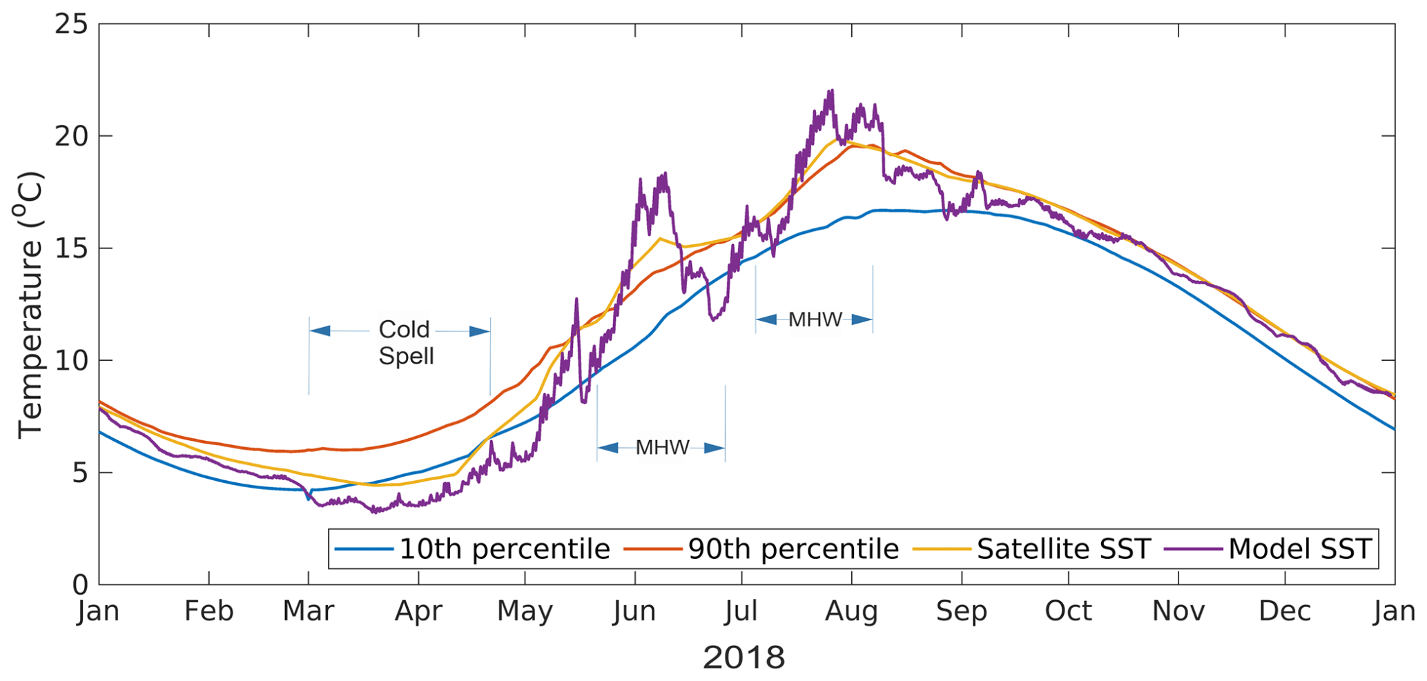
Figure 4Annual SST variation (in ∘C) at the NSB III platform in 2018. In addition to the satellite measurements (yellow curve) and the simulation results (purple curve), the 10th and 90th percentile SSTs from the multiyear statistics are shown. One cold spell and two MHWs were detected based on the 10th and 90th percentiles.
Regarding the relationship between air temperature variations and the seasonal cyclicity of the thermal stratification, further comparisons were made among a typical normal year (i.e. 2015), the extreme heat wave year of 2018, and the multiyear mean (Fig. 5). In the warm season of 2018, there were three periods in which the air temperature was higher than the multiyear mean. The maximum air temperature anomaly reached 6∘C. Correspondingly, three “heat spikes” are present on the SST curve. During each of these three periods, the SST sharply increased, whereas the water temperature in the deeper layers hardly changed. In 2015, the SST “heat spikes” were associated with rapidly increasing air temperatures from June to July; however, in contrast to the summer of 2018, the summer of 2015 was colder than the warm season average, with the maximum air temperature anomaly being 3 ∘C lower than the multiyear mean.
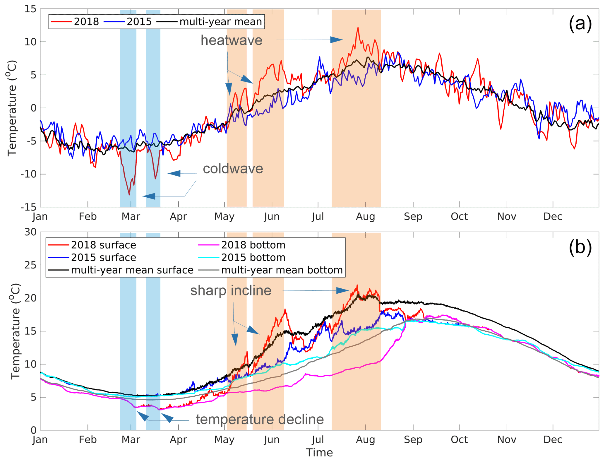
Figure 5(a) Annual variation in the simulated air temperature (with the multiyear mean removed) at NSB III for 2018 (red line), 2015 (blue line) and the multiyear mean (black line). In the warm season of 2018, the periods in which the air temperature was higher than the multiyear mean and the SST increased are delineated with orange frames. Likewise, in the early spring of 2018, the periods in which the air temperature was lower than the multiyear mean and the SST decreased are delineated with blue frames. (b) Similar to (a) but for the simulated water temperature at the surface and the bottom.
In the absence of turbulent mixing, high air temperatures (warmer summers) lead to high SSTs and intensify the local surface–bottom temperature differences. This is evident in the three “heat spike” periods in 2018. Note that the first “heat spike” in 2018 was not identified as an MHW event due to the relatively low temperatures. In 2015, no atmospheric heat wave or MHW events were detected. Correspondingly, the SST was below the average, and the surface–bottom temperature difference was smaller than the multiyear mean.
Seawater exhibits a longer memory of low temperatures than the atmosphere; this leads to a larger and more stable thermal stratification. As shown in Fig. 5, at the end of February into mid-March 2018, there were two cold spells with air temperatures 7 ∘C lower than the multiyear mean. In response, the seawater was colder than usual, causing the bottom temperature to be 2 ∘C lower than the average. This low temperature signal remained much longer in the water than in the atmosphere and yielded colder bottom temperatures over the entire warm season.
The monthly mean spatial distribution of ϕ in the southern North Sea in 2018 (Fig. 6) provides an overview of the seasonal cycle of thermal stratification development during extreme temperature events. The water column was considered to be stratified when ϕ exceeds 50 J m−3, which implies the amount of energy required to instantaneously homogenize a 60 m deep water column with a surface–bottom density difference of 1 kg m−3, where 60 m is approximately the average water depth of the North Sea (excluding the Norwegian Channel). The water becomes stratified by April in the northern part of the domain, i.e. to the north of the 50 m isobath, whereas to the south, density stratification hardly occurs in the winter months (December through February), except off the Dutch coast and the German Bight. The potential energy anomaly increases after April, while stratification develops in the area north of 54∘ N latitude from May to August. The potential energy anomaly reaches 400 J m−3 on average from July to early August, with a maximum value of approximately 800 J m−3 in the area between the Dogger Bank and MARNET station NSB III. In September, the 50 J m−3 isoline retreats to the north of the 50 m isobath. Moreover, south of 54∘ N latitude, the water column is mostly well mixed, and the stratification near the Dutch coast and the German Bight is attributable to river runoff.
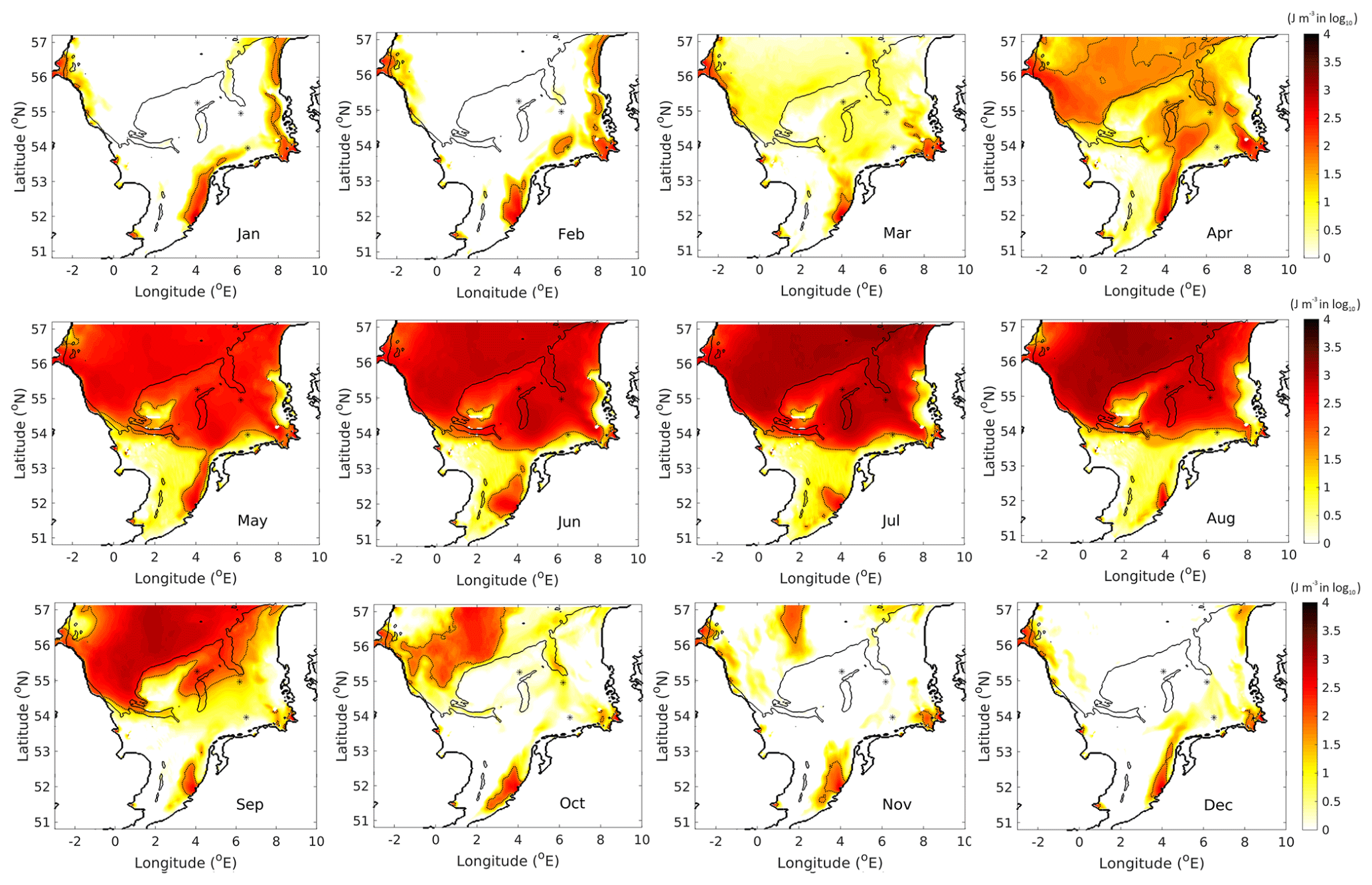
Figure 6Evolution of the monthly mean potential energy anomaly ϕ (see Eq. 1, unit: J m−3 on a log10 scale) for 2018. The dashed line indicates the location where ϕ=1.7 J m−3 on log10 scale (or ϕ=50 J m−3). The water column is considered to be stratified when ϕ is above this value. Thin black lines indicate the location of the 50 m isobath.
The intensity of the summer stratification varies over time. To illustrate the interannual variability of the water stratification in the southern North Sea, the potential energy anomaly of each year relative to the multiyear mean (2011–2018) is computed by averaging the anomalies over a 3-month period from June to August (the main stratification period, see Fig. 6). The results are shown in Fig. 7. In 2013, 2014 and 2018, the stratification is stronger than the average, whereas, in the other years the stratification is weaker. In the areas where the water depth is shallower than 50 m, the largest interannual variation occurs between 3 and 8∘ E longitude and north to 54∘ N latitude. The mean potential energy anomaly is 300–400 J m−3 higher than the multiyear mean in 2018, while it is 200–300 J m−3 lower than average in 2015. Note that the largest interannual variations in the stratification occur in the eastern part of the southern North Sea.
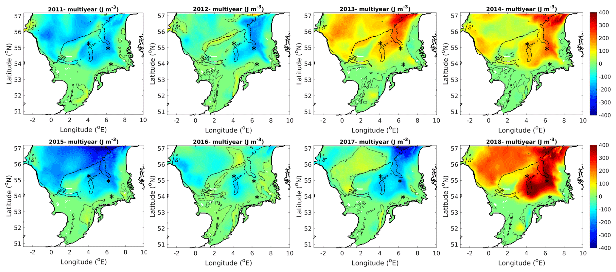
Figure 7Difference in the potential energy anomaly (J m−3) averaged over 3 months (June, July and August) between a specific year and the multiyear mean. The dashed line indicates ϕ=50 J m−3. Thin black lines indicate the location of the 50 m isobath.
As illustrated in Figs. 6 and 7, the stratification/destratification process in the North Sea was temporally and spatially dependent. The data analysed at a single point were incapable of revealing a complete image of the relationship between the seasonal thermal stratification and the varying air temperatures in the North Sea. van Leeuwen et al. (2015) investigated the physical conditions in the North Sea and attributed regimes of different types of stratification to thermally induced, salt-induced, river-induced and turbulent tidal mixing. They found that in the southern North Sea, a large area could not be characterized by a dominant physical mechanism. Focusing on thermally induced stratification, the relation between the variation in air temperature and the seasonal thermal stratification in the North Sea was analysed. The correlation coefficient R reflecting the linear correlation between the air temperature and the potential energy anomaly for the summer of 2018 was computed, and its distribution is mapped in Fig. 8. High coefficients (R>0.8) were obtained mainly in the middle and northern parts of the North Sea (Fig. 8a). This area is consistent with the regime of seasonal stratification identified in van Leeuwen et al. (2015). Closer to the coast, lower R values were obtained and five scattered locations in the southern North Sea were selected regarding the different values of R (see Fig. 8a) based on the air temperature versus potential energy anomaly (Fig. 8b). Note that both the Dogger Bank and the NSB III site are located in the region for which the stratification type was unclassified in van Leeuwen et al. (2015). A linear correlation existed between the increase in air temperature and the increasing stratification, with R=0.8 at the Northsea Mid site and R=0.7 at the Dogger Bank. The larger potential energy anomalies in the middle and northern North Sea (see “Northsea Mid” in Fig. 8a) were attributed to the deeper water depths therein. At NSB III, R=0.5 similarly reflects a linear increase in stratification with the air temperature. Off the Dutch Coast and along the Norwegian Trench, R was negative; at the former location, the water column was stratified due to river runoff, while at the latter, the water was permanently stratified. The potential energy anomaly was not correlated with the air temperatures at the two locations.
Mapping the correlation between the air temperature and the potential energy anomaly for different years yielded similar spatial patterns and values of R in the North Sea except for the middle part of the southern North Sea, where lower R values were found for the years with relatively cold summers. For example, in 2015, R fell by 0.1–0.3 in the area between the Dogger Bank and NSB III (not shown), indicating a much lower correlation between the summer stratification and air temperature.
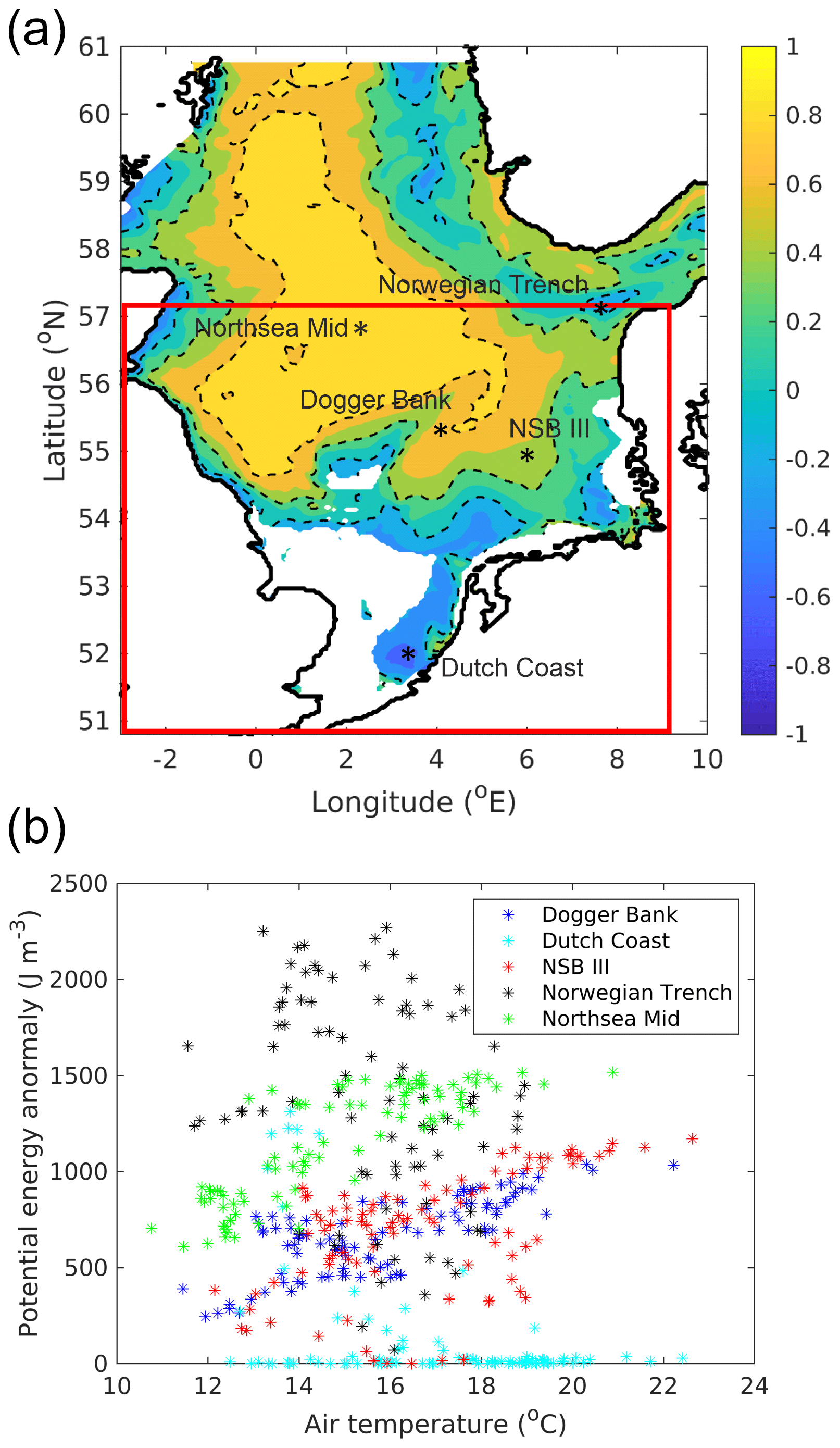
Figure 8(a) Computed correlation coefficient R between the air temperature and the potential energy anomaly for summer 2018 (June, July and August). Note that the area with no stratification (ϕ<50 J m−3) is excluded. Dashed contours indicate and 0.8. (b) Relationship between the air temperature and the potential energy anomaly in the different regimes of the North Sea. The locations are illustrated in (a). The red frame indicates the region of the southern North Sea.
Similar to Fig. 4, the MHW events for each warm season (1 May–31 August) during the simulation period 2011–2018 were detected, and the number of MHW days (ℳ) was counted. Then, the changes in ℳ with respect to its multiyear mean were computed for the modelling period. Here, “” denotes the number of years, and an overline denotes the multiyear mean. Similarly, the number of days (𝒩) that the water column was stratified () and the changes in stratified days were computed. Finally, the sensitivity of stratification to the occurrence of heat waves was quantified with the ratio r between the change in the number of heat wave days and the change in the number of water stratification days:
Note that the region where no MHW events were detected (ℳ=0) was not considered. Figure 9 shows the spatial distribution of r in the North Sea, where r varies between 0 and 1. When r=0, the number of days when the water column is stratified does not change interannually. This pattern occurs for both permanently stratified regions and permanently mixed regions. The former was found in the Norwegian Trench and the latter was found mainly in the western part of the southern North Sea, as well as in the shallow shoal of the Dogger Bank, along the Danish coast and in the southern part of the German Bight. In contrast, when r=1, the change in the number of water stratification days equals the change in the number of MHW days, which illustrates the dependence of the thermal stratification on the occurrence of MHWs. In the region where the water depth is greater than 50 m, r<0.2. This region is consistent with the region where R>0.6, where stratification occurs seasonally with annually varying air temperatures. South of the 50 m isobath, r>0.3 and increases towards the coasts, indicating an enhanced influence of MHWs on water stratification. The region where r peaked was between 6.5∘ E and the Danish coast. It is worth noting that an MHW causes density stratification within the water column, and that the resulting stratification hampers the transfer of heat along the water column and intensifies the occurrence of an MHW.
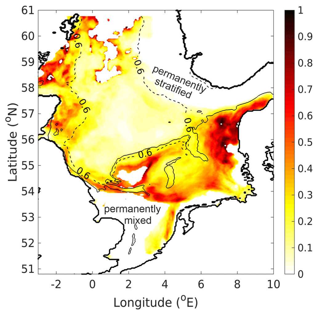
Figure 9Ratio of the number of water stratification days to the number of MHW days. The dashed contour line corresponds to the correlation coefficient R=0.6 between the air temperature and the potential energy anomaly for the multiyear mean of the summer time. The thin solid line indicates the 50 m isobath.
Large values of r were also observed between the MHW-induced stratification region and the permanently mixed region and near the United Kingdom coastline in the northern North Sea. These regions are shallow and mostly mixed by tides. The water stratification is due to the short and intensive increase in air temperature. As shown in Fig. 5, three periods of stratification (ϕ>50 J m−3) were detected. Similar to how MHW days were counted, the number of days from May to August during 2011–2018 in which the air temperature sharply increased were obtained. In the present study, the criterion was set to 0.2 ∘C d−1, i.e. the air temperature increase rate was at least two times larger than the rate of increase in the multiyear mean averaged over the warm season (see Fig. 5, upper panel). After applying Eq. (6), the ratio between the change in the number of days in which the air temperature intensively increases and the change in the number of water stratification days was obtained (see Fig. 10). Overall, the spatial distribution of this ratio was similar to that of the ratio between the changes in the numbers of MHW and water stratification days. This was particularly true in the area adjacent to the tidal mixing zone and the MHW-induced stratification zone; this region is consistent with the intermittently stratified domain characterized by van Leeuwen et al. (2015). It is also important to stress the role of the winter–spring cold spell, which reduces the SST (see Fig. 4), thus increasing the vertical instability of the water column and enhancing vertical mixing. This results in the seawater being colder than average before the summer temperature rises, especially in the deeper water layers, via the redistribution of the heat through the water column. Hence, a more persistent thermal stratification is likely to be obtained in the southern North Sea.
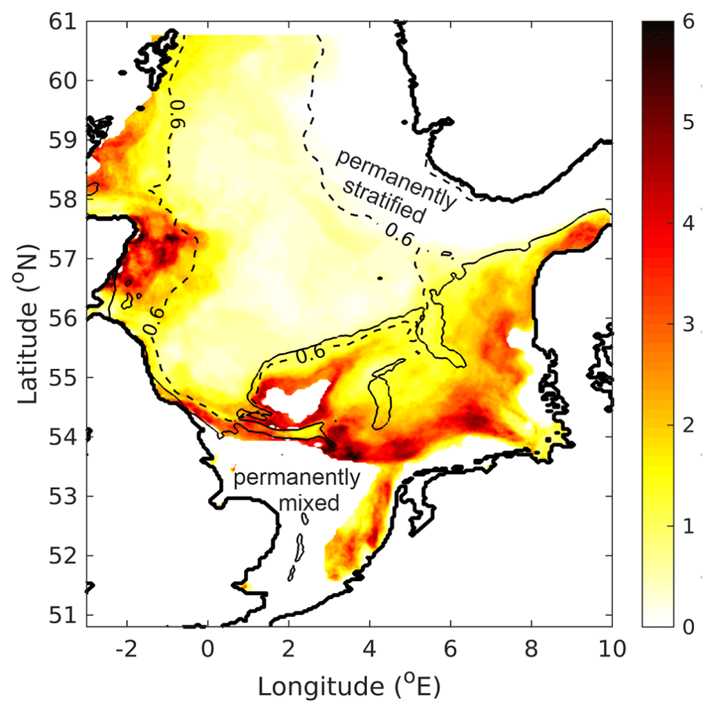
Figure 10Ratio between the number of days when the water is stratified and the number of days when the air temperature intensively increases. The dashed contour line with a value of 0.6 indicates the area with a correlation coefficient R=0.6 between the air temperature and the potential energy anomaly for the multiyear mean of the summertime. The thin solid line indicates the 50 m isobath.
The sensitivity of thermal stratification to the occurrence of an MHW was related to changes in water depth. Figure 11 presents the annual variation in the gradient Richardson number Ri for the selected stations with different depths in the regime where R≥0 (see Fig. 8). The water column was considered stably stratified when log10(Ri)≥1; i.e. the buoyancy was an order of magnitude larger than the vertical shear. In both 2015 and 2018, the water column became stratified from May to September in the middle of the North Sea, exhibiting comparable values of Ri. Approaching the coast (with decreasing water depth), Ri decreases. At Fino-1, the water column was mostly well-mixed, despite some intermittent stratifications on the time scale of 1–2 d. Differences between 2015 and 2018 were observed at the Dogger Bank and at NSB III. In the Dogger Bank, stratification occurred from June to the end of August in 2015, which was both shorter and less intensive than the same period in 2018. At NSB III, stable stratification existed only in 2018.
Further analysis of the vertical distribution of Ri revealed that the maximum value of Ri was obtained in the middle of the water column. At the Northsea Mid, the peak was located at a depth of approximately 35 m. Below 45 m, log10(Ri)∼0, and the water column was homogeneous throughout the entire year. At NSB III, the period in which large Ri values were recorded was consistent with the occurrence of MHW events. In 2018, log10(Ri)≥1 during June and from early July to August. Moreover, in the Dogger Bank and at NSB III, the maximum Ri shifted from the upper water layers to the bottom during the early stage of the warm season; however, in the late warm season (July and August), the maximum Ri remained in the middle water layers. At both Dogger Bank and NSB III, the water column below 25 m was homogeneous throughout the entire year. At Fino-1, the water depth (25 m) was too shallow to maintain long-term stable stratification.
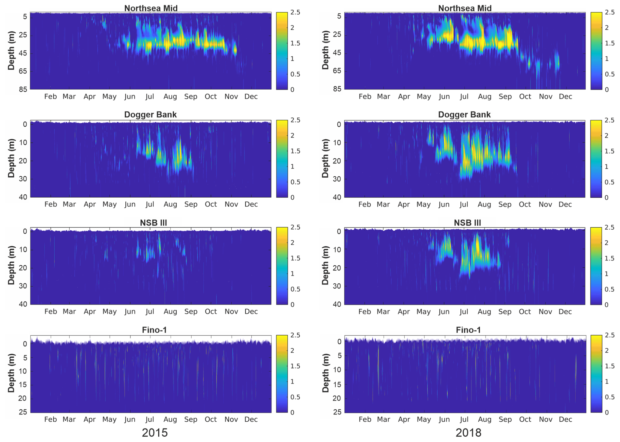
Figure 11Gradient Richardson numbers Ri for 2015 (left column) and 2018 (right column) at the Northsea Mid, Dogger Bank, NSB III and Fino-1 on a log10 scale.
Note that the present study takes into account the impact of ocean waves on circulation. Such an impact usually results from different processes, e.g. turbulence due to breaking or non-breaking waves and the transfer of momentum from breaking waves to currents (Davies et al., 2000; Babanin, 2006; Breivik et al., 2015). The latter is important in shallow waters such as the Baltic Sea (Alari et al., 2016) and the North Sea (Staneva et al., 2017; Wu et al., 2019). By including wave-induced turbulent mixing, the simulation was capable of resolving the turbulent mixing length and modelling the vertical stratification and circulation in the North Sea (Staneva et al., 2017, 2021), especially near the coastal zones. Figure 12 shows the modelled seasonal mean mixed layer depth (MLD) of the coupled NEMO-WAM model run in 2018 and the relative changes when comparing the fully coupled run with the uncoupled run, i.e. . Following the annual water temperature cycle, the MLD in the southern North Sea decreases from winter to summer and rises again in autumn. The MLD changes more quickly in deeper regions than in shallow coastal areas. There is almost no seasonal cycle along the coast of the German Bight. The large difference in the MLD between the coupled and uncoupled runs is found from spring to autumn, when stratification develops with the changing air temperature. In summer, the MLD of the coupled run is approximately 20 %–40 % larger than that of the uncoupled run in the southern North Sea, whereas it is approximately 20 % smaller north up to the 54∘ N latitude. In autumn, the stratification disappears in the southern North Sea, where the MLD differences drop between −10 % and 10 %. In the north, where the water depth is deeper than 50 m, the MLD of the coupled run is approximately 20 % larger than the MLD of the uncoupled run.
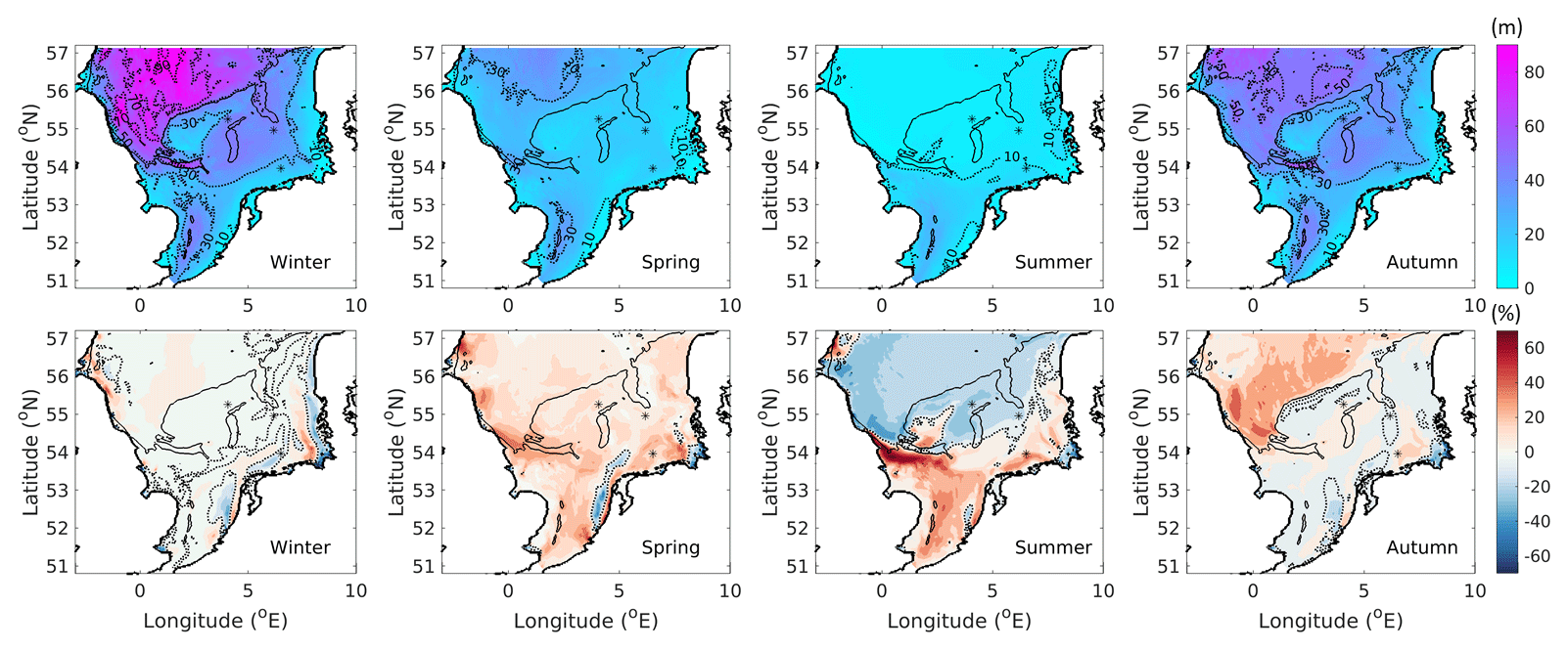
Figure 12Upper panels: the seasonal mean mixed layer depth (MLD) of the coupled NEMO-WAM model run. Lower panels: the relative changes in the MLD when comparing the coupled run with the stand-alone NEMO (uncoupled) run. Dotted lines in the lower panels indicate the 0 % contour.
Wave-induced processes also change the heat fluxes at the water surface (Fig. 13). The net heat flux is positive overall (from the air to the sea) in spring and summer and negative (from the sea to the air) in winter and autumn. The importance of wave forcing for ocean predictions in the North Sea has been demonstrated by Staneva et al. (2017). Wave-induced processes impact the distribution of the heat fluxes. In summer, in the southern North Sea, the fluxes increase by approximately 20 %–40 %, while a reduction of 20 %–50 % occurs along the coastal, well-mixed area of the German Bight. For further details of these wave impacts, refer to the Supplement for the results of the model run where NEMO was uncoupled with WAM.
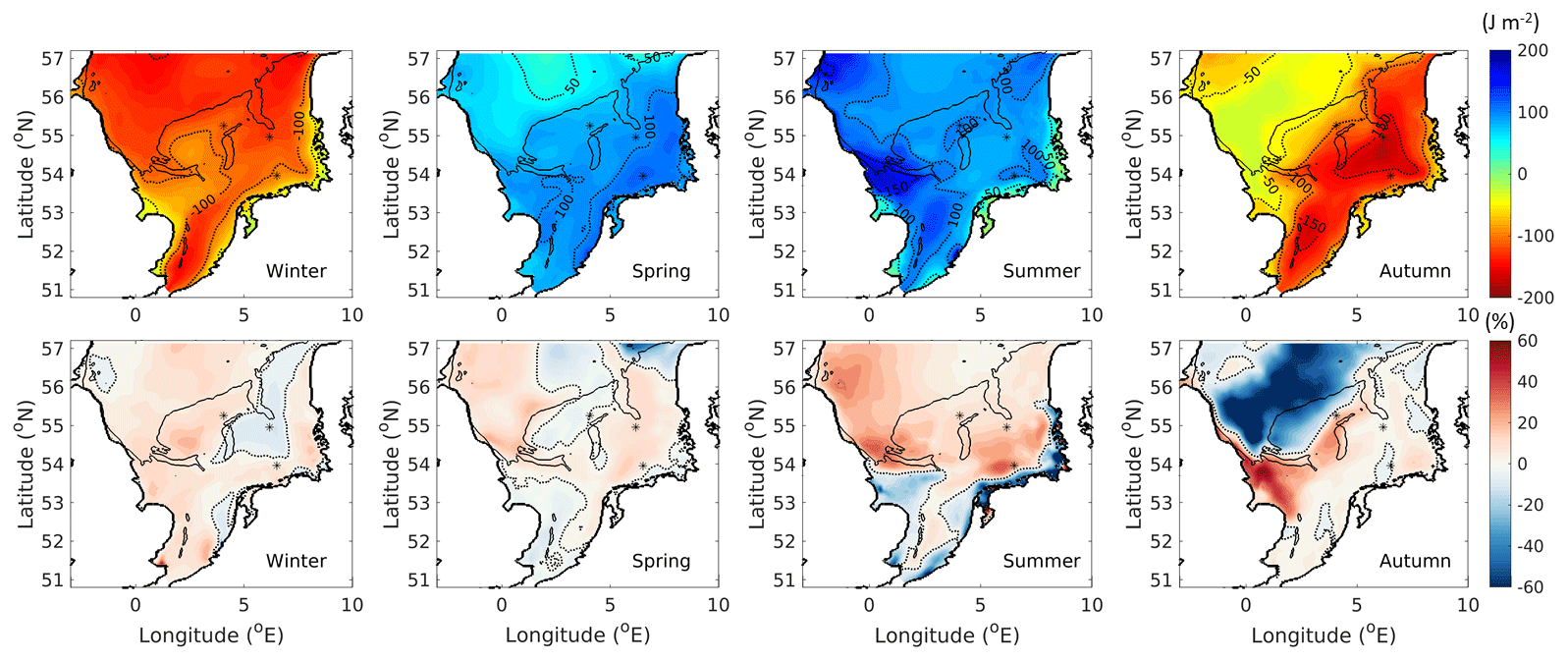
Figure 13Same as Fig. 12, but for the surface heat fluxes. In the upper panels, positive values denote net fluxes from the air to the sea.
Apart from circulation-wave coupling, the stratification itself also influences the circulation. Baroclinic circulation, a result of the balance between baroclinic forcing and friction, becomes more pronounced with stronger current velocities (larger vertical shear) under warmer conditions when the turbulent eddy viscosity is eliminated by the increased stratification. Huang et al. (1999) showed that water transport in the Bohai Sea is enhanced from weak stratification in spring to strong stratification in summer. In the North Sea, the relations between the cycle of thermal fronts and baroclinic circulation were analysed at different timescales (Lwiza et al., 1991; Luyten et al., 1999). Decreased vertical turbulent mixing reduces the magnitude and horizontal shear of baroclinic currents. This was found to be important feedback from turbulent mixing to the frontal temperature gradients and baroclinic circulation (Luyten et al., 2003) and these mechanisms become further pronounced when extreme meteorological events occur. By analysing 40 years of data, Schrum et al. (2003) identified an unusual stratification due to wind and volume transport in the 1990s. Recently, Chen et al. (2021) investigated the heat budget of the North Sea and demonstrated that the modification of SST affects the advection of water and transport of heat in the North Sea. Comparatively, extreme events, e.g. summer heat waves, have more intensive influences on SST, albeit on a shorter timescale. Exploring the responses of the regional water circulation to extreme events in the southern North Sea is certainly an interesting topic and deserves further study.
This study investigated the influence of extreme meteorological events, e.g. European heat waves, on the occurrence of the summer stratification in the North Sea. With a numerical model that simulated the water temperatures over multiple years, this work addressed the question remaining after the study by van Leeuwen et al. (2015): what kind of “interannual variability” results in the failure to classify the stratification regimes in one third of the North Sea?
Based on the model simulations, a potential energy anomaly was calculated for multiple years in the North Sea model domain. In the southern North Sea, stratification developed from May to August. The intensity of this stratification presented an obvious interannual variation that was related to the occurrence of summer heat wave events. The data from 2018 were analysed as a case study and compared with the multiyear mean and the data during a normal year (i.e. 2015). Regarding the main factors that affect the intensity and duration of the thermal stratification in the southern North Sea, the comparison of temperature data near the water surface and the bottom revealed three aspects. The first was the intense increase in SST over a short time, the second was a higher water temperature during summer than the multiyear mean, and the third was the memory of the near-bottom water layer to the low air temperatures during early spring.
By computing the correlation coefficient (R) between the air temperatures and the potential energy anomaly, the region of thermal stratification in the North Sea was identified (R>0). This region covers the North Sea north of 54∘ N , excluding the permanently stratified Norwegian Trench and the permanently well-mixed coastal seas near the Danish Wadden Sea. The features of this stratification differed between the northern and southern sides of 54∘ N at a depth of 50 m. In contrast to the northern part, where the water column was seasonally stratified every year, the southern part was stratified in the years when heat waves occurred. The dependence of thermal stratification on heat wave events was quantified by the ratio r between the change in the number of water stratification days in 2011–2018 and the change in the number of MHW days during the same period. A ratio r=1 indicates that the change in the number of thermal stratification days is the same as that of MHW days. Large ratios (r>0.8) were found to the south of the 50 m isobath (between 6.5∘ E and the Danish coast), covering most of the region left with an unclassified stratification regime by van Leeuwen et al. (2015).
Water depth appeared to be the factor that controlled the sensitivity of the stratification to summer heat wave events. In addition to the proximity to the coast, the stratification period was highly dependent on the number of days a heat wave event lasted. After analysing the structure of the gradient Richardson number Ri, it was found that heat wave-induced seasonal stratification occurred mainly in the region where the water depth is between 35 and 50 m.
This research is the first to link heat wave events to the occurrence and persistence of density stratification in the southern North Sea. In a broader context, this research is expected to have fundamental significance for further investigating the secondary effects of heat wave events, such as in ecosystems, fisheries, and sediment dynamics. With the growing debate regarding the impacts of increasingly extreme meteorological events, future assessments of these factors will be of only growing importance in the North Sea.
The water density ρ in Eq. (2) is given by
In the above equation, S is the salinity of seawater in parts per thousand by volume (ppt). The reference density ρr and the coefficients A, B and C are also functions of the potential temperature T (∘C) following the expressions given by Millero and Poisso (1981):
Here, S and T are obtained from the model with a temporal resolution of 6 h. Moreover, the 6 h resolution model output of the sea surface elevation η is taken for computation (see Eqs. 1 and 2 in the main text).
The model code is available at https://www.nemo-ocean.eu/ for NEMO (NEMO, 2022; https://doi.org/10.5281/zenodo.6334656, Gurvan et al., 2022) and https://github.com/mywave/WAM (Behrens, 2022) for WAM.
The outputs of the GCOAST simulations (in NetCDF format) are available upon request to the corresponding author.
The supplement related to this article is available online at: https://doi.org/10.5194/nhess-22-1683-2022-supplement.
WC wrote the article and analysed and interpreted the results. WC and JS conceived the study. SG ran the simulations and was responsible for all technical issues of the modelling. JS and JSS contributed to the writing. JG performed the field work and collected observational data.
The contact author has declared that neither they nor their co-authors have any competing interests.
Publisher’s note: Copernicus Publications remains neutral with regard to jurisdictional claims in published maps and institutional affiliations.
This article is part of the special issue “Coastal hazards and hydro-meteorological extremes”. It is not associated with a conference.
The authors gratefully acknowledge the German Climate Computing Centre (DKRZ) for providing computing time on the Supercomputer MISTRAL. We acknowledge the Cluster of Excellence EXC 2037 “Climate, Climatic Change, and Society” (CLICCS) (project no. 390683824). Wei Chen acknowledges the EU H2020 project DOORS (grant no. 101000518). Joanna Staneva acknowledges the European Green Deal project “Large scale RESToration of COASTal ecosystems through rivers to sea connectivity” (REST-COAST) (grant no. 101037097). Sebastian Grayek gratefully acknowledges funding from the EU H2020 project IMMERSE (grant no. 821926).
This research has been supported by the bilateral BMBF project “Ocean Currents_MoDA” (grant no. 03F0822A) and the Helmholtz-Gemeinschaft (grant no. Digital Earth).
The article processing charges for this open-access publication were covered by the Helmholtz-Zentrum Hereon.
This paper was edited by Agustín Sánchez-Arcilla and reviewed by two anonymous referees.
Alari, V., Staneva, J., Breivik, Ø., Bidlot, J.-R., Mogensen, K., and Janssen, P.: Surface wave effects on water temperature in the Baltic Sea: simulations with the coupled NEMO-WAM model, Ocean Dynam., 66, 917–930, https://doi.org/10.1007/s10236-016-0963-x, 2016. a
Babanin, A. V.: On a wave-induced turbulence and a wave-mixed upper ocean layer, Geophys. Res. Lett., 33, L20605, https://doi.org/10.1029/2006GL027308, 2006. a
Becker, G. A.: Beiträge zur hydrographie und wärmebilanz der Nordsee, Deutsche Hydrografische Zeitschrift, 34, 167–262, https://doi.org/10.1007/BF02225959, 1981. a
Behrens, A.: Third generation spectral wave model WAM Cycle 6, GitHub [code], https://github.com/mywave/WAM, last access: 11 May 2022. a
Bensoussan, N., Romano, J. C., Harmelin, J. G., and Garrabou, J.: High resolution characterization of northwest Mediterranean coastal waters thermal regimes: to better understand responses of benthic communities to climate change, Estuar. Coast. Shelf S., 87, 431–441, https://doi.org/10.1016/j.ecss.2010.01.008, 2010. a
Bond, N. A., Cronin, M. F., Freeland, H., and Mantua, N.: Causes and impacts of the 2014 warm anomaly in the NE Pacific, Geophys. Res. Lett, 42, 3414–3420, https://doi.org/10.1002/2015GL063306, 2015. a
Borges, A., Royer, C., Martin, J. L., Champenois, W., and Gypens, N.: Response of marine methane dissolved concentrations and emissions in the Southern North Sea to the European 2018 heatwave, Cont. Shelf Res., 190, 104004, https://doi.org/10.1016/j.csr.2019.104004, 2019. a
Breivik, Ø., Mogensen, K., Bidlot, J. R., Balmaseda, M. A., and Janssen, P. A. E. M.: Surface wave effects in the NEMO ocean model: Forced and coupled experiments, J. Geophys. Res., 120, 2973–2992, https://doi.org/10.1002/2014JC010565, 2015. a
Chen, W., Schulz-Stellenfleth, J., Grayek, S., and Staneva, J.: Impacts of the assimilation of satellite sea surface temperature data on volume and heat budget estimates for the North Sea, J. Geophys. Res.-Oceans, 126, e2020JC017059, https://doi.org/10.1029/2020JC017059, 2021. a, b, c
Davies, A. M., Kwong, S. C. M., and Flather, R. A.: On determining the role of wind wave turbulence and grid resolution upon computed storm driven currents, Cont. Shelf Res., 20, 1825–1888, https://doi.org/10.1016/S0278-4343(00)00052-2, 2000. a
Egbert, G. D. and Erofeeva., S. Y.: Efficient inverse modeling of barotropic ocean tides, J. Atmos. Ocean. Tech., 19, 183–204, 2002. a
Elliott, A. and Clarke, T.: Seasonal stratification in the northwest European shelf seas, Cont. Shelf Res., 11, 467–492, https://doi.org/10.1016/0278-4343(91)90054-A, 1991. a
Feng, M., McPhaden, M., Xie, S., and Hafner, J.: La Niña forces unprecedented Leeuwin Current warming in 2011, Sci. Rep.-UK, 3, 1277, https://doi.org/10.1038/srep01277, 2013. a
Fernand, L., Weston, K., Morris, T., Greenwood, N., Brown, J., and Jickells, T.: The contribution of the deep chlorophyll maximum to primary production in a seasonally stratified shelf sea, the North Sea, Biogeochemistry, 113, 153–166, https://doi.org/10.1007/s10533-013-9831-7, 2013. a
Fettweis, M., Baeye, M., Van der Zande, D., Van den Eynde, D., and Joon Lee, B.: Seasonality of floc strength in the southern North Sea, J. Geophys. Res.-Oceans, 119, 1911–1926, https://doi.org/10.1002/2013JC009750, 2014. a
GEOMAR: RV Poseidon Fahrtbericht/Cruise Report POS526, GEOMAR Helmholtz-Zentrum für Ozeanforschung, Kiel, Germany, GEOMAR Report, N. Ser. 051, 86 pp. https://doi.org/10.3289/geomar_rep_ns_51_2019, 2019. a
Günther, H., Hasselmann, S., and Janssen, P. A. E. M.: The WAM model, Cycle 4, Hamburg, 26, 109 pp., 1992. a
Gurvan, M., Bourdallé-Badie, R., Chanut, J., Clementi, E., Coward, A., Ethé, C., Iovino, D., Lea, D., Lévy, C., Lovato, T., Martin, N., Masson, S., Mocavero, S., Rousset, C., Storkey, D., Müeller, S., Nurser, G., Bell, M., Samson, G., Mathiot, P., Mele, F., and Moulin, A.: NEMO ocean engine, in: Notes du Pôle de modélisation de l'Institut Pierre-Simon Laplace (IPSL) (v4.2.0, Number 27), Zenodo [code], https://doi.org/10.5281/zenodo.6334656, 2022. a
Herring, S. C., Hoerling, M. P., Kossin, J. P., Peterson, T. C., and Stott, T. C.: Introduction to explaining extreme events of 2014 from a climate perspective, B. Am. Meteorol. Soc., 96, S1–S4, 2015. a
Hersbach, H., Bell, B., Berrisford, P., Hirahara, S., Horányi, A., Muñoz-Sabater, J., Nicolas, J., Peubey, C., Radu, R., Schepers, D., Simmons, A., Soci, C., Abdalla, S., Abellan, X., Balsamo, G., Bechtold, P., Biavati, G., Bidlot, J., Bonavita, M., De Chiara, G., Dahlgren, P., Dee, D., Diamantakis, M., Dragani, R., Flemming, J., Forbes, R., Fuentes, M., Geer, A., Haimberger, L., Healy, S., Hogan, R. J., Hólm, E., Janisková, M., Keeley, S., Laloyaux, P., Lopez, P., Lupu, C., Radnoti, G., de Rosnay, P., Rozum, I., Vamborg, F., Villaume, S., and Thépaut, J.: The ERA5 global reanalysis, Q. J. Roy. Meteor. Soc., 146, 1999–2049, 2020. a
Hill, A. E., James, I. D., Linden, P. F., Matthews, J. P., Prandle, D., Simpson, J. H., Gmitrowicz, E. M., Smeed, D. A., Lwiza, K. M. M., Durazo, R., and Fox, A. D.: Dynamics of tidal mixing fronts in the North Sea, In: Understanding the North Sea System, Springer, Dordrecht, 53–68, https://doi.org/10.1007/978-94-011-1236-9_5, 1994. a
Hobday, A. J. and Pecl, G. T.: Identification of global marine hotspots: sentinels for change and vanguards for adaptation action, Rev. Fish Biol. Fisher., 24, 415–425, https://doi.org/10.1007/s11160-013-9326-6, 2014. a
Hobday, A. J., Alexander, L. V., Perkins, S. E., Smale, D. A., Straub, S. C., Oliver, E. C. J., Benthuysen, J. A., Burrows, M. T., Donat, M. G., Feng, M., Holbrook, N. J., Moore, P. J., Scannell, H. A., Sen Gupta, A., and Wernberg, T.: A hierarchical approach to defining marine heatwaves, Prog. Oceanogr., 141, 227–238, https://doi.org/10.1016/j.pocean.2015.12.014, 2016. a, b, c
Ho-Hagemann, H. T. M., Gröger, M., Rockel, B., Zahn, M., Geyer, B., and Meier, H.: Effects of air-sea coupling over the North Sea and the Baltic Sea on simulated summer precipitation over Central Europe, Clim. Dynam., 49, 3851–3876, https://doi.org/10.1007/s00382-017-3546-8, 2017. a
Hu, Z., Kumar, A., Jha, B., Zhu, J., and Huang, B.: Persistence and predictions of the remarkable warm anomaly in the northeastern Pacific Ocean during 2014–16, J. Climate, 30, 689–702, https://doi.org/10.1175/JCLI-D-16-0348.1, 2017. a, b
Huang, D., Su, J., and Backhaus, J. O.: Modelling the seasonal thermal stratification and baroclinic circulation in the Bohai Sea, Cont. Shelf Res., 19, 1485–1505, https://doi.org/10.1016/S0278-4343(99)00026-6, 1999. a
Imbery, F., Friedrich, K., Haeseler, S., Koppe, C., Janssen, W., and Bissolli, P.: Vorläufiger Rückblick auf den Sommer 2018 –eine Bilanz extremer Wetterereignisse, Tech. rep., Deutscher Wetterdienst (DWD), https://www.dwd.de/DE/leistungen/besondereereignisse/temperatur/20180803_bericht_sommer2018.pdf (last access: 3 May 2022), 2018. a
IPCC: AR6 Climate Change 2021: The Physical Science Basis, Cambridge University Press, in press, 2022. a
Klonaris, G., Van Eeden, F., Verbeurgt, J., Troch, P., Constales, D., Poppe, H., and De Wulf, A.: ROMS Based Hydrodynamic Modelling Focusing on the Belgian Part of the Southern North Sea, J. Mar. Sci. Eng., 9, 58, https://doi.org/10.3390/jmse9010058, 2021. a
Luyten, P., Jones, J., Proctor, R., Tabor, A., Tett, P., and Wild-Allen, K.: COHERENS – A coupled hydrodynamical–ecological model for regional and shelf seas: User documentation, Management Unit of the Mathematical Models of the North Sea (MUMM), 914 pp., 1999. a
Luyten, P. J., Jones, J. E., and Proctor, R.: A numerical study of the long-and short-term temperature variability and thermal circulation in the North Sea, J. Phys. Oceanogr., 33, 37–56, https://doi.org/10.1175/1520-0485(2003)033<0037:ANSOTL>2.0.CO;2, 2003. a, b, c
Lwiza, K., Bowers, D., and Simpson, J.: Residual and tidal flow at a tidal mixing front in the North Sea, Cont. Shelf Res., 11, 1379–1395, https://doi.org/10.1016/0278-4343(91)90041-4, 1991. a
Madec, G. and the NEMO team: NEMO ocean engine, Note du Pole de modélisation, Institut Pierre-Simon Laplace (IPSL) No. 27, France, ISSN 1288-1619, https://www.nemo-ocean.eu/doc/ (last access: 3 May 2022), 2016. a
Manta, G., de Mello, S., Trinchin, R., Badagian, J., and Barreiro, M.: The 2017 record marine heatwave in the southwestern Atlantic shelf, Geophys. Res. Lett., 45, 12449–12456, https://doi.org/10.1029/2018GL081070, 2018. a
Mathis, M., Elizalde, A., Mikolajewicz, U., and Pohlmann, T.: Variability patterns of the general circulation and sea water temperature in the North Sea, Prog. Oceanogr., 135, 91–112, https://doi.org/10.1016/j.pocean.2015.04.009, 2015. a
Merchant, C. J., Embury, O., Bulgin, C. E., Block, T., Corlett, G. K., Fiedler, E., Good, S. A., Mittaz, J., Rayner, N. A., Berry, D., Eastwood, S., Taylor, M., Tsushima, Y., Waterfall, A., Wilson, R., and Donlon, C.: Satellite-based time-series of sea-surface temperature since 1981 for climate applications, Scientific Data, 6, 223, https://doi.org/10.1038/s41597-019-0236-x, 2019. a
Millero, F. J. and Poisso, A.: International one-atmosphere equation of state of seawater, Deep Sea Research Part A: Oceanographic Research Papers, 28, 625–629, https://doi.org/10.1016/0198-0149(81)90122-9, 1981. a, b
NEMO: Nucleus for European Modelling of the Ocean, European consortium, https://www.nemo-ocean.eu/, last access: 11 May 2022. a
Nielsen, T. G., Løkkegaard, B., Richardson, R., Pedersen, F. B., and Hansen, L.: Structure of plankton communities in the Dogger Bank area (North Sea) during a stratified situation, Mar. Ecol.-Prog. Ser., 95, 115–131, a
O’Dea, E. J., Arnold, A. K., Edwards, K. P., Furner, R., Hyder, P., Martin, M. J., Siddorn, J. R., Storkey, D., While, J., Holt, J. T., and Liu, H.: An operational ocean forecast system incorporating NEMO and SST data assimilation for the tidally driven European North-West shelf, J. Oper. Oceanogr., 5, 3–17, https://doi.org/10.1080/1755876X.2012.11020128, 2012. 1993. a
Oliver, E., Benthuysen, J. A., Bindoff, N. L., Hobday, A. J., and J.Holbrook, N.: The unprecedented 2015/16 Tasman Sea marine heatwave, Nat. Commun., 8, 16101, https://doi.org/10.1038/ncomms16101, 2017. a, b
Oliver, E. C., Benthuysen, J. A., Darmaraki, S., Donat, M. G., Hobday, A. J., Holbrook, N. J., Schlegel, R. W., and Gupta, A. S.: Marine heatwaves, Annu. Rev. Mar. Sci., 13, 313–342, https://doi.org/10.1146/annurev-marine-032720-095144, 2020. a, b
Otto, L., Zimmerman, J. T. F., Furnes, G. K., Mork, M., Sætre, R., and Becker, G.: Review of the physical oceanography of the North Sea, Neth. J. Sea Res., 26, 161–238, https://doi.org/10.1016/0077-7579(90)90091-T, 1990. a
Pearce, A., Lenanton, R., Jackson, G., Moore, J., Feng, M., and Gaughan, D.: The “marine heat wave” off Western Australia during the summer of 2010/11, Fisheries Research Report No. 222, Department of Fisheries, Western Australia, 40pp., https://www.fish.wa.gov.au/documents/research_reports/frr222.pdf, 2011. a
Perkins, S. E. and Alexander, L. V.: On the measurement of heat waves, J. Climate, 26, 4500–4517, https://doi.org/10.1175/JCLI-D-12-00383.1, 2013. a
Perkins-Kirkpatrick, S., King, A. D., Cougnon, E. A., Grose, M. R., Oliver, E. C. J., Holbrook, N., Lewis, S., and Pourasghar, F.: The role of natural variability and anthropogenic climate change in the 2017/18 Tasman Sea marine heatwave, B. Am. Meteorol. Soc, 100, S105–10, https://doi.org/10.1175/BAMS-D-18-0116.1, 2019. a
Pingree, R. and Griffiths, D.: Tidal fronts on the shelf seas around the British Isles, J. Geophys. Res.-Oceans, 83, 4615–4622, https://doi.org/10.1029/JC083iC09p04615, 1978. a
Pohlmann, T.: Calculating the development of the thermal vertical stratification in the North Sea with a three-dimensional baroclinic circulation model, Cont. Shelf Res., 16, 163–194, https://doi.org/10.1016/0278-4343(95)00018-V, 1996. a
Rouault, M., Illig, S., Bartholomae, C., Reason, C., and Bentamy, A.: Propagation and origin of warm anomalies in the Angola Benguela upwelling system in 2001, J. Mar. Syst., 68, 473–488, https://doi.org/10.1016/j.jmarsys.2006.11.010, 2007. a
Sas, H., Didderen, K., van der Have, T., Kamermans, P., van den Wijngaard, K., and Reuchlin-Hugenholtz, E.: Recommendations for flat oyster restoration in the North Sea, Tech. rep., Sas Consultancy, https://www.ark.eu/sites/default/files/media/Schelpdierbanken/Recommendations_for_flat_oyster_restoration_in_the_North_Sea.pdf (last access: 3 May 2022), 2019. a
Schrum, C., Siegismund, F., and St John, M.: Decadal variations in the stratification and circulation patterns of the North Sea. Are the 1990s unusual, in: ICES Marine Science Symposia, vol. 219, Oxford University Press, 121–131, 2003. a, b
Sharples, J., Ross, O. N., Scott, B. E., Greenstreet, S. P. R., and Fraser, H.: Inter-annual variability in the timing of stratification and the spring bloom in the North-western North Sea, Cont. Shelf Res., 26, 733–751, 2006. a, b
Simpson, J. H.: The shelf-sea fronts: implications of their existence and behaviour, Philos. T. R. Soc. Lond., 302, 531–546, https://doi.org/10.1098/rsta.1981.0181, 1981. a
Smale, D. A., Wernberg, T., Oliver, E. C. J., Thomsen, M., Harvey, B. P., Straub, S. C., Burrows, M. T., Alexander, L. V., Benthuysen, J. A., Donat, M. G., Feng, M., Hobday, A. J., Holbrook, N. J., Perkins-Kirkpatrick, S. E., Scannell, H. A., Gupta, A. S., Payne, B. L., and Moore, P. J.: Marine heatwaves threaten global biodiversity and the provision of ecosystem services, Nat. Clim. Change, 9, 306–312, https://doi.org/10.1038/s41558-019-0412-1, 2019. a
Staneva, J., Alari, V., Breivik, O., Bidlot, J. R., and Mogensen, K.: Effects of wave-induced forcing on a circulation model of the North Sea, Ocean Dynam., 67, 81–191, https://doi.org/10.1007/s10236-016-1009-0, 2017. a, b, c, d
Staneva, J., Ricker, M., Carrasco-Alvarez, R., Breivik, Ø., and Schrum, C.: Effects of Wave-Induced Processes in a Coupled Wave–Ocean Model on Particle Transport Simulations, Water, 13, 473–488, https://doi.org/10.3390/w13040415, 2021. a, b
Stathopoulos, C., Galanis, G., and Kallos, G.: A coupled modeling study of mechanical and thermodynamical air-ocean interface processes under sea storm conditions, Dynam. Atmos. Oceans, 91, 101140, https://doi.org/10.1016/j.dynatmoce.2020.101140, 2020. a
Stips, A., Bolding, K., Pohlmann, T., and Burchard, H.: Simulating the temporal and spatial dynamics of the North Sea using the new model GETM (general estuarine transport model), Ocean Dynam., 54, 266–283, https://doi.org/10.1007/s10236-003-0077-0, 2004. a, b
Tan, H. and Cai, R.: What caused the record-breaking warming in East China Seas during August 2016?, Atmos. Sci. Lett., 19, 853, https://doi.org/10.1002/asl.853, 2018. a
The Wamdi Group: The WAM Model – A Third Generation Ocean Wave Prediction Model, J. Phys. Oceanogr., 18, 1775–1810, https://doi.org/10.1175/1520-0485(1988)018<1775:TWMTGO>2.0.CO;2, 1988. a
Umlauf, L. and Burchard, H.: A generic lengthscale equation for geophysical turbulence models, J. Mar. Res., 61, 235–265, https://doi.org/10.1357/002224003322005087, 2003. a
van Haren, H.: Properties of vertical current shear across stratification in the North Sea, J. Mar. Res., 58, 465–491, https://doi.org/10.1357/002224000321511115, 2000. a
van Leeuwen, S., Tett, P., Mills, D., and van der Molen, J.: Stratified and nonstratified areas in the North Sea: Long-term variability and biological and policy implications, J. Geophys. Res.-Oceans, 120, 4670–4686, https://doi.org/10.1002/2014JC010485, 2015. a, b, c, d, e, f, g, h
Wakelin, S., Townhill, B., Engelhard, G., Holt, J., and Renshaw, R.: Marine heatwaves and cold-spells, and their impact on fisheries in the southern North Sea, EGU General Assembly 2021, online, 19–30 Apr 2021, EGU21-7329, https://doi.org/10.5194/egusphere-egu21-7329, 2021. a, b, c
Wernberg, T., Smale, D. A., Tuya, F., Thomsen, M. S., Langlois, T. J., De Bettignies, T., Bennett, S., and Rousseaux, C. S.: An extreme climatic event alters marine ecosystem structure in a global biodiversity hotspot, Nat. Clim. Change, 3, 78–82, https://doi.org/10.1038/NCLIMATE1627, 2013. a
Wernberg, T., Bennett, S., Babcock, R. C., De Bettignies, T., Cure, K., Depczynski, M., Dufois, F., Fromont, J., Fulton, C. J., Hovey, R. K., et al.: Climate-driven regime shift of a temperate marine ecosystem, Science, 353, 169–172, https://doi.org/10.1126/science.aad8745, 2016. a
Wu, L., Staneva, J., Breivik, O., Rutgersson, A. adn George Nurser, A. J., Clementi, E., and Madec, G.: Wave effects on coastal upwelling and water level, Ocean Model., 140, 101405, https://doi.org/10.1016/j.ocemod.2019.101405, 2019. a
- Abstract
- Introduction
- Materials and methods
- Results
- Discussion
- Conclusions
- Appendix A: Estimates of the seawater density
- Code availability
- Data availability
- Author contributions
- Competing interests
- Disclaimer
- Special issue statement
- Acknowledgements
- Financial support
- Review statement
- References
- Supplement