An ensemble of state-of-the-art ash dispersion models: towards probabilistic forecasts to increase the resilience of air traffic against volcanic eruptions

High-quality volcanic ash forecasts are crucial to minimize the economic impact of volcanic hazards on air traffic. Decision-making is usually based on numerical dispersion modelling with only one model realization. Given the inherent uncertainty of such an approach, a multi-model multi-source term ensemble has been designed and evaluated for the Eyjafjallajökull eruption in May 2010. Its use for flight planning is discussed. Two multi-model ensembles were built: the first is based on the output of four dispersion models and their own implementation of ash ejection. All a priori model source terms were constrained by observational evidence of the volcanic ash cloud top as a function of time. The second ensemble is based on the same four dispersion models, which were run with three additional source terms: (i) a source term obtained from a model background constrained with satellite data (a posteriori source term), (ii) its lower-bound estimate and (iii) its upper-bound estimate. The a priori ensemble gives valuable information about the probability of ash dispersion during the early phase of the eruption, when observational evidence is limited. However, its evaluation with observational data reveals lower quality compared to the second ensemble. While the second ensemble ash column load and ash horizontal location compare well to satellite observations, 3D ash concentrations are negatively biased. This might be caused by the vertical distribution of ash, which is too much diluted in all model runs, probably due to defaults in the a posteriori source term and vertical transport and/or diffusion processes in all models. Relevant products for the air traffic management are horizontal maps of ash concentration quantiles (median, 75 %, 99 %) at a finely resolved flight level grid as well as cross sections. These maps enable cost-optimized consideration of volcanic hazards and could result in much fewer flight cancellations, reroutings and traffic flow congestions. In addition, they could be used for route optimization in the areas where ash does not pose a direct and urgent threat to aviation, including the aspect of aeroplane maintenance.

1 Introduction

Volcanic eruptions that spread out ash over large areas can have tremendous economic consequences, although they are relatively rare compared to other high-impact natural hazards (such as tropical cyclones, storms, etc). For instance, the eruption of Eyjafjallajökull in 2010 forced the cancellation of about 100 000 flights and generated a EUR 1.4 billion loss to the airline operators (IATA, 2010). Considering the different levels of risks to safety when an aircraft encounters ash, including failure of aircraft turbines during operation (Guffanti et al., 2010; Alexander, 2013), flight cancellations and reroutings out of the ash-contaminated areas were the most common decision during this eruption.

In order to mitigate the consequences of such types of volcanic eruptions on aviation, operational centres continuously watch possible volcanic eruptions and issue warnings about ash dispersion in the atmosphere, which support the decisions in the frame of predefined procedures (Bolić and Sivčev, 2011). This watching and warning role worldwide has been the duty of Volcanic Ash Advisory Centres (VAACs). Following the consequences of the Eyjafjallajökull eruption in Europe, the London and Toulouse VAACs' procedures have changed, and they now also provide concentration charts in the flight level (FL) bands FL000-200, FL200-350, and FL350-550 for three contamination levels: 0.2 to 2 mg m⁻³ (low contamination), 2 to 4 mg m⁻³ (medium contamination), and $>\mathrm{4}\mathrm{mg}{\mathrm{m}}^{-\mathrm{3}}$ (high contamination) (ICAO, 2016). These volcanic ash contamination charts (up to 18 h ahead) indicate hazardous zones and hazard levels, which can be used by authorities for flight safety.

Volcanic ash warnings and charts are based on the outputs from numerical prediction models. As a consequence, they are usually prone to large errors and uncertainties (Kristiansen et al., 2012; Dacre et al., 2016), which arise from the uncertainties in the ash source term, in the modelling of transport including meteorology, and in the parameterization of physical processes. Although these components have been improving thanks to active research (Beckett et al., 2020), it is highly probable that predictions with sufficient accuracy cannot be reached in the near future. The ash source term, i.e. the temporal evolution of volcanic ash mass emitted by the volcano at every vertical level and distributed over aerosol size groups, cannot be fully observed, and even after inversion of satellite observations some error and uncertainty remain (Kristiansen et al., 2012). Aerosol processes (sedimentation, washout and rainout, aggregation in the presence of liquid or solid water) and aerosol transport depend on the aerosols' representation in the model, and also on the meteorological conditions. The meteorological forecasts, for which error grows inevitably with time (Dacre et al., 2016) and which are essential input information for ash dispersion forecasts, also contribute significantly to uncertainties in ash forecasts. In order to account for the uncertainty of volcanic ash forecasts, some studies have already shown the added value of ensembles (Kristiansen et al., 2012). Consequently, they recommended using probabilistic forecasts in the decision process (Prata et al., 2019), in a similar manner as probabilistic meteorological weather forecasts, which have shown to have a large benefit compared to deterministic forecasts (Richardson, 2000; Osinski and Bouttier, 2018; Fundel et al., 2019).

Proof-of-concept studies for flight planning are in progress (Steinheimer et al., 2016) to use probabilistic meteorological forecasts to support aviation safety, capacity, and cost-efficiency. Regarding volcanic ash hazards, interest in ensemble prediction is also increasing among the meteorological operational community (such as VAACs). Beyond the important safety aspect, one potential application of probabilistic ash forecasts is related to ash dosage (i.e. the accumulated mass of ash encountered by the aircraft along its track), which is an important parameter to characterize the impact of ash on aircraft engines (Clarkson et al., 2016). While accumulated long-term exposure of ash at lower concentrations can also be a safety issue (e.g. 1 mg m⁻³ for about 3 h), low ash doses can lead to long-term damage to the engines and may require shorter maintenance intervals in order to prevent performance loss (Clarkson et al., 2016). Contaminated regions can be avoided by flight rerouting, but this increases costs due to delays and additional fuel. As a consequence, a cost $/$ loss ratio (Richardson, 2000) can be considered in regions where ash concentrations remain below the safety margins, and in that sense, probabilistic ash forecasts (Prata et al., 2019) could be used to make optimal decisions for air traffic management (ATM). Such applications require good estimates of ash concentrations in four dimensions (3D space and time) as well as their uncertainty. Overall, cost-optimized consideration of volcanic hazards based on ensemble dispersion modelling could result in a significantly reduced impact on flight cancellations, rerouting, and traffic flow congestion during volcanic ash events (Rokitansky et al., 2019).

In the European Natural Airborne Disaster Information and Coordination System for Aviation (EUNADICS-AV) project, a multi-model approach has been developed and assessed on several test cases. The outputs from several models were collected to build a mini-ensemble and probabilistic charts of ash concentrations. This ensemble has a 0.1^∘ horizontal resolution for a large Euro-Atlantic domain, and provides information on 13 vertical FLs. The integration of these data into a flight-planning software and their relevance for ATM were shown during an exercise simulating a fictitious crisis situation (Hirtl et al., 2020).

The purpose of the present article is to provide more precise understanding of the performance and benefit of the multi-model multi-source-term ensemble approach developed during the EUNADICS-AV project, using measurements as a reference for comparison. The performance of individual model runs performed with four models using four different source terms each is also evaluated to better understand ensemble characteristics and benefits. The uncertainty of the meteorological conditions was not taken into account; i.e. meteorological analyses were concatenated with short-term forecasts.

The study focuses on a particular period of the Eyjafjallajökull eruption from 13 to 20 May 2010, when ash spread across the North Sea and the Atlantic Ocean, and then over continental Europe. During this period, the number of measurements was particularly high compared to other phases of the eruption. Dacre et al. (2016) pointed out a low predictability of the dispersion of ash during this period, and they studied how the error grew with time. Their study emphasized the need for ensemble approaches in order to deal with uncertainty. For the same phase of the eruption, Kristiansen et al. (2012) compared two different models with different source terms. They showed overall a good agreement between models, and that the ensemble obtained as the mean ash concentration of the different models (a mean ensemble) usually, but not generally, outperforms any of the models.

The outline of the present article is as follows: Sect. 2 gives a description of the models, the source terms, and the reference data. Section 3 compares the model outputs and evaluates them against reference observations. Section 4 presents how mini-ensembles are built and compares them to reference observations as well. Section 5 discusses how such an ensemble can be used in flight planning for future eruptions. Conclusions are drawn in Sect. 6.

2 Models and observations

2.1 Ash dispersion models

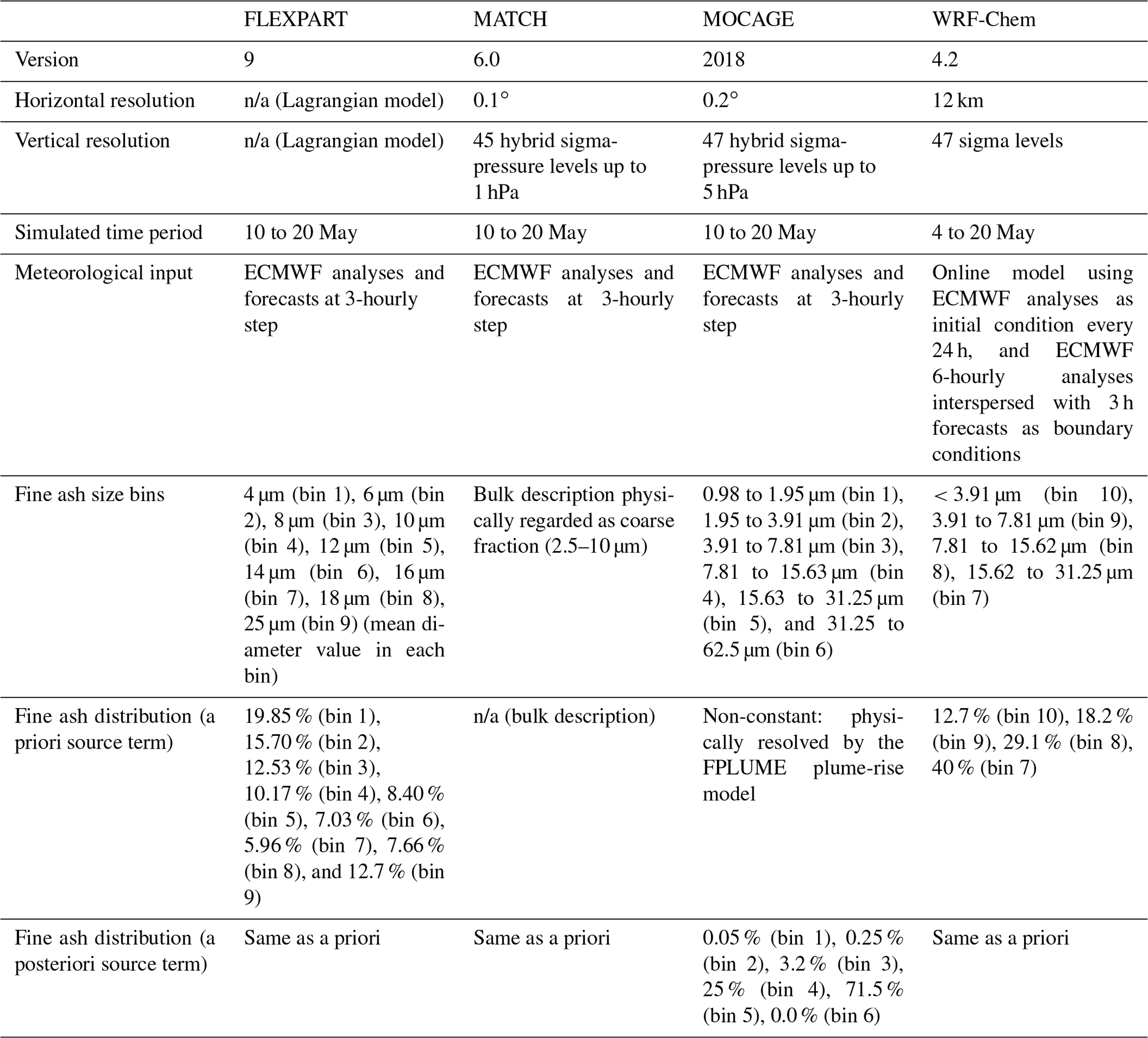
The four models used in the present study are shortly described below. These models are different by design (i.e. some are chemistry transport or on-line coupled models, and some are Lagrangian or Eulerian), and they have different aerosol schemes, which brings in a pragmatic consideration for some of the uncertainties, regardless of the limited number of models. A general presentation of each model is given, particularly regarding the representation of transport and of ash processes. Then the simulation designs for the case study are summarized in Table 1. The source terms are described in a following section (Sect. 2.2).

Table 1 Summary of the model configurations used for the model simulations.

2.1.1 FLEXPART (ZAMG)

The FLEXPART Lagrangian particle dispersion model is a widely used multi-scale atmospheric transport modelling and analysis tool, operated both in the research and in operational domains since its start back in the 1990s. In particular, at ZAMG (Zentralanstalt für Meteorologie und Geodynamik, the Austrian Weather Service), FLEXPART (Stohl et al., 1998, 2005; Pisso et al., 2019) is not only used to operationally assist the Austrian government in its nuclear emergency response activities but also to predict dispersion of volcanic ash and SO₂ worldwide. It considers transport, mixing, gravitational settling, dry and wet deposition, radioactive decay, and simple linearized chemical reactions of gases. To model ash dispersion over Europe in this study, the convection parameterization (Forster et al., 2007) was activated. Sub-grid-scale terrain parameterization was enabled, which increases the mixing heights due to sub-grid-scale orographic deviations deduced from the European Centre for Medium-Range Weather Forecasts (ECMWF) input field “standard deviation of orography”.

2.1.2 MATCH (SMHI)

MATCH is a comprehensive Eulerian chemical transport model for operation and research activities in a wide range of applications (Robertson et al., 1999; Andersson et al., 2007). This includes nuclear emergencies, volcanic eruptions, and tropospheric chemistry modelling. The MATCH model has been applied for resolutions down to 500 m and up to the global scale. The model describes all transport phases like advection, diffusion, sedimentation, and wet and dry deposition and includes wet and dry chemistry and advanced codes for aerosol modelling of mineral dust and of secondary inorganic aerosols (sulfate, nitrate, and ammonia) and secondary organic aerosols (formed from organic gases) (Andersson et al., 2015). In this application aerosols are described with a single bin, given deposition and optical properties of aerosols with a prescribed size distribution.

2.1.3 MOCAGE (Météo-France)

MOCAGE is a chemistry-transport model that is used for operational and research applications at Météo-France for air quality purposes. A light version of MOCAGE has also been developed and used for emergency dispersion modelling, including the ash forecasts operated by the Toulouse VAAC. The MOCAGE configuration used in the present study complies with the one described by Guth et al. (2016): it enables full tropospheric and stratospheric chemistry, primary aerosols (desert dust, sea salt, volcanic ash, black carbon, and organic carbon), and secondary aerosols (sulfate, nitrate, and ammonium). The aerosol scheme represents various processes, as described by Guth et al. (2016): transport (advection and sub-grid transport), sedimentation, deposition (dry and wet), and interaction with gas-phase chemistry.

2.1.4 WRF-Chem (ZAMG)

The online-coupled chemical transport model WRF-Chem (Grell et al., 2005) is operationally used at ZAMG for air quality prediction over Europe with a special focus on Austria. This model simulates the emission, transport, mixing, and chemical reactions of trace gases and aerosols as well as meteorological conditions. The following physical model options were used: the two-moment cloud microphysics scheme (Morrison et al., 2009), Rapid Radiative Transfer Method for Global (RRTMG) long-wave and short-wave radiation (Iacono et al., 2008), Grell 3D cumulus parameterization (Grell and Freitas, 2014), NOAH land surface model (Chen and Dudhia, 2001), and Mellor–Yamada–Nakanishi–Niino (MYNN) level 2.5 planetary boundary layer (PBL) scheme (Nakanishi and Niino, 2004).

All model simulations start from 10 May or before, which includes a spin-up phase of at least 3 d. The main objective of the spin-up is to assure that ash from the most recent phase of the eruption is present in the domain. From 9 to 12 May, the emission was rather low and constant. Considering the size of the domain and the intensity of ash emission, 3 d is a reasonable time frame to allow realistic background ash concentrations in the domain for the model. WRF-Chem used a 9 d spin-up, but it has been checked whether the differences of results between WRF-Chem and the other models are not attributed to different spin-up lengths.

All model outputs are post-processed every hour, on the same $\mathrm{0.1}{}^{\circ }\times \mathrm{0.1}{}^{\circ }$ latitude–longitude grid, by interpolating the values horizontally, and to 13 vertical layers, by calculating the mean concentration of fine volcanic ash between the corresponding FLs.

2.2 Source terms

Every model uses two types of source terms: an a priori source term and an a posteriori source term. A priori source terms are computed from simple schemes, e.g. using data such as plume height estimates as input information. An a priori approach may simulate the diversity of source terms that could be used as a first approach in real time, such as every centre uses its own source term. The a posteriori source term was obtained after inversion of satellite total column estimates (Stohl et al., 2011).

For all models, the a priori source terms are, in a nutshell, derived from a plume model using plume height estimates from radar data (Arason et al., 2011). The plume models are respectively PLUMERIA (Mastin, 2007) for FLEXPART, FPLUME (Folch et al., 2016) for MOCAGE, and the Mastin et al. (2009) relationship, which empirically relates plume height with emitted mass per time step, for MATCH and WRF-Chem. MATCH and WRF-Chem assume an umbrella-shaped plume with slightly different structures: while MATCH assigns 10 % of the mass to below 25 % of the plume height, 15 % of the mass up to 50 % of the plume height, and the remaining 75 % of the mass to above 50 % of the plume height, WRF-Chem assigns 25 % of the mass from the vent height to the umbrella base (75 % of the plume-top height) and 75 % of the mass to the umbrella (Stuefer et al., 2013; Hirtl et al., 2019). Furthermore, radar plume heights used in both models were slightly different. The records of radar plume heights used in MATCH are those reported at the time of the Eyjafjallajökull eruption. Reports were provided for various durations from 3 to 21 h (in steps of 3 h). Some longer durations may just be a concatenation of repeated height levels in consecutive reports. For WRF-Chem, the 75 % quantile of plume-top altitude statistics calculated for 3 h time intervals and provided by Arason et al. (2011) is used.

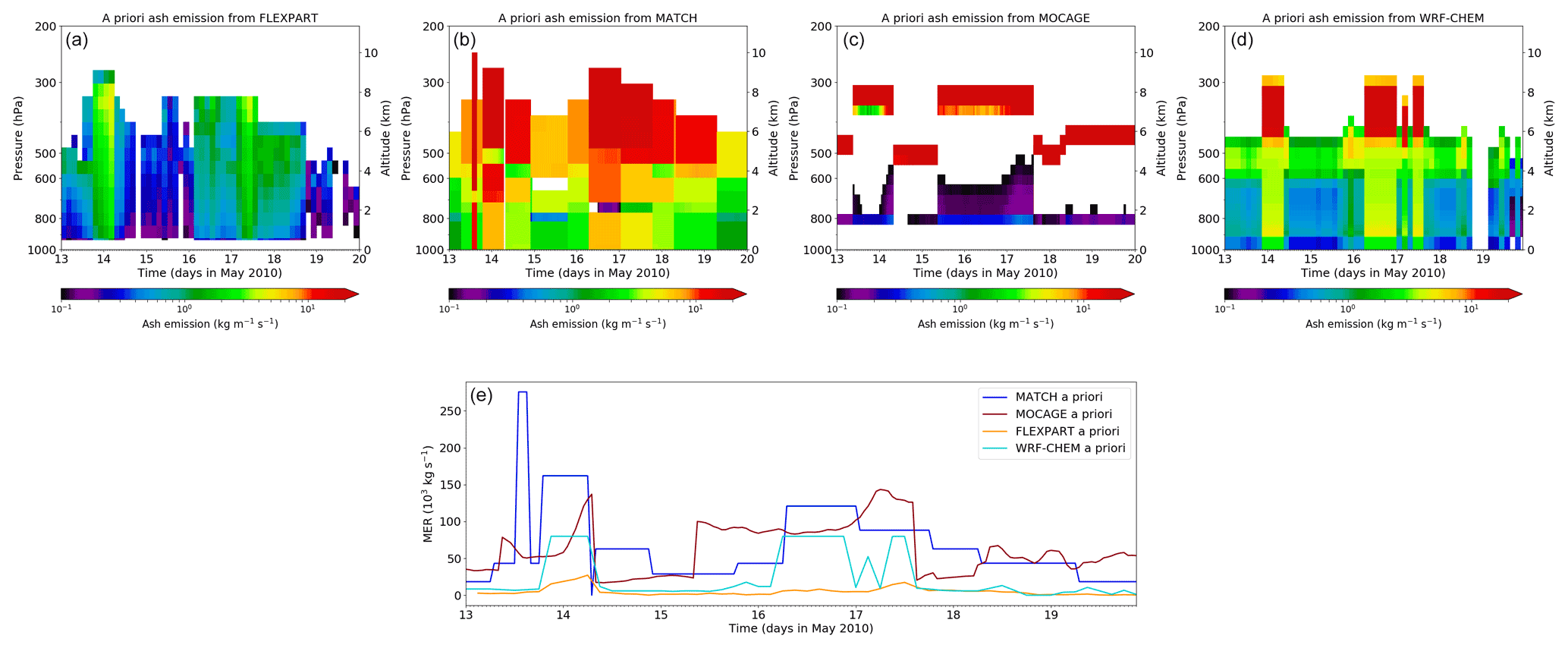
Figure 1 (a–d) A priori source terms used for FLEXPART, MATCH, MOCAGE, and WRF-Chem (from left to right). The source terms of fine ash are expressed in $\mathrm{kg}{\mathrm{m}}^{-\mathrm{1}}{\mathrm{s}}^{-\mathrm{1}}$ and are shown as a function of time and height. (e) Mass eruption rate (unit kg s⁻¹) for the four source terms, as a function of time.

The time–height evolution of the source term intensity differs significantly from one model to the other (Fig. 1). The same is true for the mass eruption rate (MER). Even with two source terms (MATCH and WRF-Chem) are based on the Mastin et al. (2009) relationship, the differences in MER may be explained by different assumptions used for the computation of the source terms: the fraction of fine ash that is kept from the total mass erupted, the eruption height that is assumed as entry of the models, and some parameters such as the density of ash for instance. The FPLUME–MOCAGE MER generally follows a similar order of magnitude with these two source terms based on Mastin et al. (2009). However, the FLEXPART a priori simulation, based on the PLUMERIA model, has a lower MER than the other models.

While all source terms emit most ash at high altitudes (Fig. 1), FPLUME–MOCAGE emits very little ash at medium levels and only little ash near the ground. The transition from high to low emissions is smoother for the other models. Furthermore, topography of the volcanic vent, which is actually located at 1666 m above sea level (a.s.l.), is fully considered in FPLUME–MOCAGE and FLEXPART but neglected in MATCH and WRF-Chem.

Contrary to the a priori source terms, the a posteriori source term is the same for all models. Described by Stohl et al. (2011), it is based on a Bayesian inverse modelling approach using FLEXPART in forward mode to establish the sensitivities between the emissions and the measurements. In this study, altitude and time resolved volcanic ash emissions were derived for the Eyjafjallajökull eruption in April and May 2010 using satellite observations. The data used were total column ash measurements of the Spinning Enhanced Visible and Infrared Imager (SEVIRI) aboard the geostationary Meteosat Second Generation (MSG) satellite and the Infrared Atmospheric Sounding Interferometer (IASI) aboard the polar-orbiting Metop satellite, utilizing their high temporal coverage (SEVIRI) and enhanced sensitivity to ash (IASI). Furthermore, a priori estimated ash emissions based on observed plume heights and the eruption column model PLUMERIA (Mastin, 2007) were used. Validations with independent observations revealed improved model results when using the inversion-derived a posteriori ash emission source term rather than an a priori one (Stohl et al., 2011).

Figure 2 (a–c) A posteriori source terms derived from Stohl et al. (2011): lower bound, best estimate, and upper bound (from left to right). The source terms of fine ash are expressed in $\mathrm{kg}{\mathrm{m}}^{-\mathrm{1}}{\mathrm{s}}^{-\mathrm{1}}$ and are shown as a function of time and height. (d) Mass eruption rate (unit kg s⁻¹) for the three source terms, as a function of time.

Based on an optimal estimation algorithm, the Stohl et al. (2011) source term provides an optimal value of the emission. There is, however, also uncertainty associated with the source term that is quantified as error variance after the inversion. In order to use this uncertainty, two additional source terms are built: a “lower-bound” estimate of the ash emission and an “upper-bound” estimate (Fig. 2). At each time and vertical level (t,z) above the vent, Stohl et al. (2011) provide an optimal mass estimate and its error variance (m,σ²). Lower and upper bounds are derived from the assumption that these bounds equal the 15 % and 85 % quantiles, respectively, of a log-normal distribution with maximum likelihood m and variance σ². The choice of a log-normal distribution is preferred to a normal one because it does not allow for negative values, despite the fact that the Stohl et al. (2011) inversion assumed a normal distribution of emission flux errors. The MER of these a posteriori source terms (Fig. 2) is in a similar range as the FLEXPART a priori source term, and much lower than the other a priori source terms.

2.3 VACOS reference ash observations

The algorithm Volcanic Ash Cloud properties Obtained from SEVIRI (VACOS; Piontek et al., 2021b, a) derives volcanic ash coverage, ash optical thickness at 10.8 µm, mass column loads, volcanic ash plume height, and volcanic ash effective particle radius from data of the passive SEVIRI imager aboard the geostationary MSG satellite (Schmetz et al., 2002). SEVIRI is a 12-channel instrument with a spatial resolution of 3 km at the sub-satellite point that diminishes towards the edges of the Earth disc. Its temporal resolution is 15 min in the operational mode over the Equator at 0^∘ E for the entire disc. Thus, this instrument is well-suited for the continuous monitoring of volcanic ash clouds in the atmosphere.

The VACOS retrieval of volcanic ash used here is the follow-on version of the algorithm Volcanic Ash Detection Using Geostationary Satellites (VADUGS) developed after the Eyjafjallajökull eruption in 2010 (Bugliaro et al., 2021; de Laat et al., 2020; Piontek et al., 2021b). Like other spaceborne retrievals of volcanic ash (e.g. Prata, 1989a; Prata and Grant, 2001; Francis et al., 2012; Prata and Prata, 2012; Pavolonis et al., 2013; Pugnaghi et al., 2013; Piscini et al., 2014), it exploits the spectral signatures of volcanic ash in the atmosphere, in particular the reverse absorption effect between two window channels centred at 10.8 and 12.0 µm (Prata, 1989a, b) and the information coming from all thermal SEVIRI channels. Thus, it is applicable during day and night. Moreover, VACOS uses auxiliary information like satellite viewing angle, surface temperature obtained from a numerical weather prediction (NWP) model, or clear-sky brightness temperatures derived from the SEVIRI observations. VACOS consists of four artificial neural networks (ANNs) with three hidden layers and 100 neurons each. While the development of the VADUGS and VACOS algorithms follows the ideas implemented in the related ice cloud retrievals COCS (“Cirrus Optical properties derived from CALIOP and SEVIRI algorithm during day and night”; Kox et al., 2014) and CiPS (“Cirrus Properties from SEVIRI”; Strandgren et al., 2017), the most important difference consists in the fact that the volcanic ash retrievals are trained using simulated SEVIRI thermal observations instead of collocated observations of ice clouds of the spaceborne lidar CALIPSO–CALIOP (Winker et al., 2009) as for COCS and CiPS. The VACOS input data set consists of brightness temperatures for the SEVIRI thermal channels, corresponding to observations of volcanic ash under a multitude of meteorological conditions with a multitude of microphysical and macrophysical properties like plume bottom and top height as well as volcanic ash concentrations. Ash optical properties have been computed according to a set of representative refractive indices to encompass a large variety of possible volcanic eruptions (Piontek et al., 2021c). Furthermore, VACOS is trained to detect volcanic ash in cloud-free environments and also above liquid water clouds. Ice clouds are excluded a priori through the application of the dedicated ice cloud algorithm COCS mentioned above. VACOS has a fairly good volcanic ash detection probability for ash layers with column loads between 0.2 and 1 g m⁻² (between 1 and 10 g m⁻²) of approximately 93 % (99 %) and also allows for the quantification of the ash load of the plume with a mean absolute percentage error of ca. 40 % (26 %). These values have been derived for a simulated test data set, using the retrieved ash optical depth at 10.8 µm, a typical mass extinction coefficient of 0.2 m² g⁻¹, and a threshold value of 0.2 g m⁻² (Piontek et al., 2021a).

2.4 Airborne measurements

For the period of the study, airborne measurements were reported in the literature. A lidar on board the Facility for Airborne Atmospheric Measurements (FAAM) BAe-146 research aircraft (Marenco et al., 2011) scanned ash layers to estimate ash load, ash layer height, and ash 3D concentrations above the United Kingdom and the North Sea. During the period of interest, measurements were performed on 14, 16, 17, and 18 May. Furthermore, DLR flights reported in situ estimates of 3D ash concentrations above the North Sea, Germany, and the Netherlands (Schumann et al., 2011) on 13, 16, 17, and 18 May. In the present study, these data sets are used to assess the performance of individual models and both ensembles.

2.5 Grids and post-processing

All model results were provided with hourly resolution on a common $\mathrm{0.1}{}^{\circ }\times \mathrm{0.1}{}^{\circ }$ horizontal grid from 30^∘ W to 40^∘ E in longitude and from 30 to 75^∘ N in latitude. The vertical discretization is defined by 13 flight levels from FL50 up to FL650 with 50 hectofeet (approximately 1500 m) steps. This common grid has been designed to facilitate the computation of scores on a uniform domain. The horizontal and vertical resolutions are significantly higher compared to past studies (Kristiansen et al., 2012; Dacre et al., 2016).

3 Differences between model outputs

3.1 Method and metrics

Most of the model diagnostics presented in the article are based on the model data at 0.1^∘ resolution, except for the ash location scores compared to the VACOS observations, which are calculated in a smaller domain at 0.2^∘ resolution as shown in Fig. 3. Mean values are computed to pass on the model 0.1^∘ resolution data to the 0.2^∘ resolution grid. For the 3 km resolved VACOS data, a 0.2^∘ grid cell is considered contaminated at instant H, if a 50 % fraction of VACOS pixels inside the 0.2^∘ grid box at H−15 min, H, and H+15 min are above 0.2 g m⁻². This choice has been made after some tests of different thresholds and time slots. It allows the detection of ash plumes (Fig. 3) while limiting noise and false alarms. Ash retrieval, however, is limited in the presence of clouds.

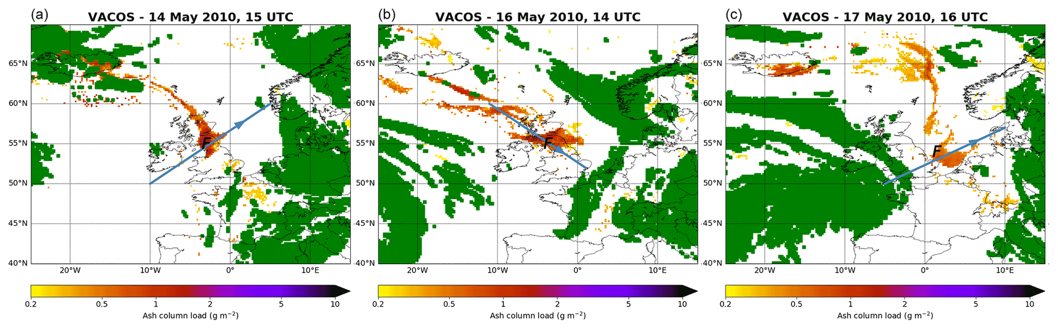
Figure 3 Ash column load retrieved from MSG/SEVIRI by the VACOS algorithm, for different dates (a–c): 14 May at 15:00 UTC, 16 May at 14:00 UTC, and 17 May at 16:00 UTC. The green zones refer to areas where the ash detection was not possible due to the presence of high clouds. The blue lines are the cross sections shown in Fig. 6, and F indicates the region where the FAAM flights made lidar measurements that are used in the article.

Figure 3 shows ash column load derived with the VACOS algorithm on several days. Ash load varies between 0.2 and 2 g m⁻². Significant amounts of ash are found close to the British north-west coast and above Scotland on 14 and 16 May, which is in good agreement with Prata and Prata (2012), who also used SEVIRI data to derive Eyjafjallajökull volcanic ash concentrations. The distribution of ash load obtained by Prata and Prata (2012) peaks at 3 g m⁻², while the VACOS ash load peaks between 1 and 2 g m⁻². Comparisons between VACOS data and ash column mass loadings derived by Francis et al. (2012) on 17 May also reveal a rather good agreement, with around 1 g m⁻² east of England. Over all dates considered, VACOS ash load is within the range of values found in the literature.

The fraction skill score (FSS) is a meaningful metric to assess the performance of volcanic ash dispersion simulations by determining the scale over which a simulation has skill for the location of ash plumes along the horizontal dimensions (Harvey and Dacre, 2016). It is calculated as

$$\begin{array}{}\text{(1)}& \text{FSS}\left(r\right)=\mathrm{1}-{\displaystyle \frac{{\sum }_{j=\mathrm{1}}^N{\left[O_j\left(r\right)-M_j\left(r\right)\right]}^{\mathrm{2}}}{{\sum }_{j=\mathrm{1}}^N\left[O_j^{\mathrm{2}}\left(r\right)+M_j^{\mathrm{2}}\left(r\right)\right]}},\end{array}$$

with N being the total number of grid points in the verification area and M_j(r) and O_j(r) being the fractions of contaminated grid points within the circle of radius r around point j, for the model and the observations, respectively. Before the computation of FSS(r), a normalization step was applied, where the G most contaminated grid points were determined for VACOS and model data. For VACOS, all grid points (within the verification area) with ash load higher than 0.2 g m⁻² are assumed to be contaminated; G is defined as the number of these grid points. For each model output, the G grid points with the highest ash column load in the domain are kept for further analysis and used to calculate the FSS. This implies that a different set of G grid points is derived compared to those determined from the VACOS data. After the normalization step, the FSS is a measure of the performance of the models to locate the most intense ash features, and it filters out the amplitude errors. In the Supplement (Fig. S7 in the Supplement), the FSS without normalization largely reflects the amplitude error of ash load. A model has skill at a given scale if the FSS is above 0.5; the higher the FSS, the better the model performance.

3.2 Ash location

Generally speaking and not surprisingly, the FSS after normalization (Fig. 4) increases with the radius of detection (50, 200, 500 km). While the models' FSSs at 50 km do not always exceed the 0.5 threshold, the FSSs at 500 km are clearly higher than 0.5, except after 19 May, when the eruption stopped and scores are less relevant. The FSSs based on the a posteriori source term (Fig. 4b, d, and e) are generally higher than the ones based on the a priori source terms, particularly for the 50 and 200 km radii. There is a large variability of scores between the models, although this variability is lower for the models with the same a posteriori source term. Snapshot ash load maps can help to analyse the FSS scores and the performances of the models and/or of the observation shortcomings, e.g. clouds hindering satellite observations.

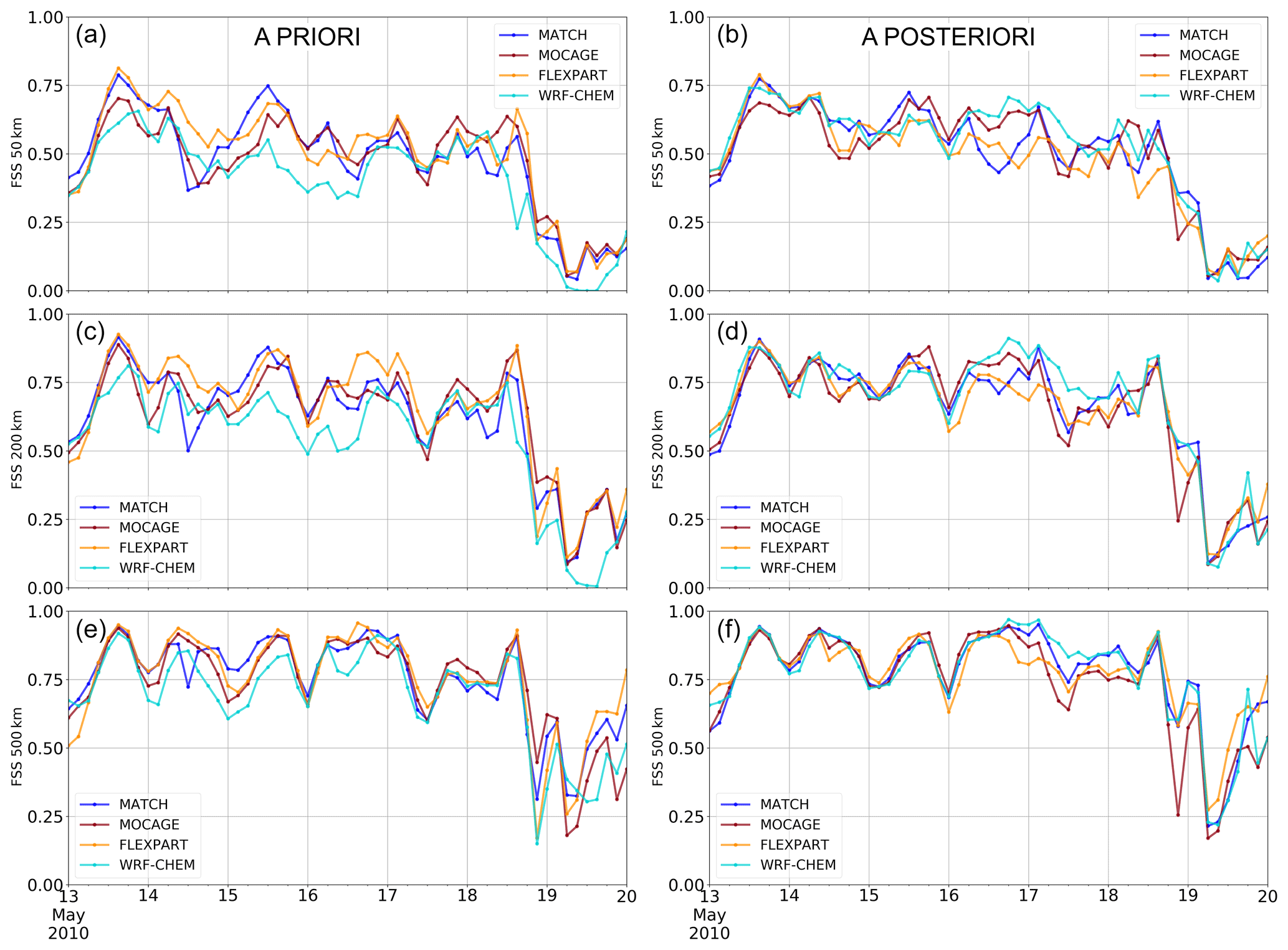
Figure 4 Comparison of the fraction skill score (FSS) for ash location, for the four models with their a priori source terms (a, c, e) and with the a posteriori source term (b, d, f). The FSS values are shown for radii of 50 (a, b), 200 (c, d), and 500 km (e, f).

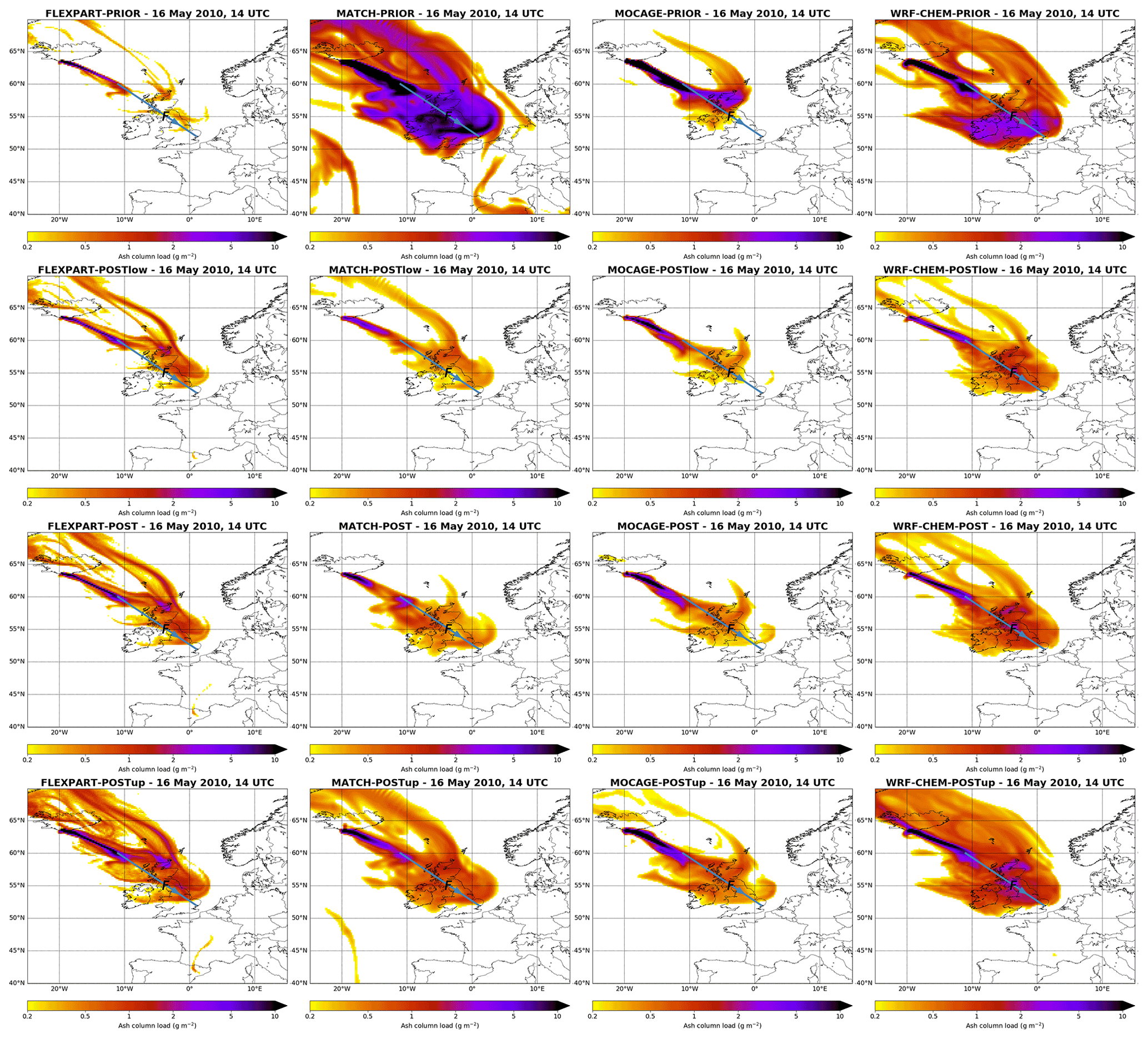
Figure 5 Ash column load on 16 May at 14:00 UTC for the four models (from left to right: FLEXPART, MATCH, MOCAGE, and WRF-Chem). The top panel shows the four model outputs with a priori source terms. The three other rows show respectively (from top to bottom) the four model outputs with the lower limit of the a posteriori source term, the best-estimate a posteriori source term, and the upper limit of the a posteriori source term. The model outputs can be compared to the observed values in Fig. 3. The blue lines are the same as in Fig. 3.

On 16 May at 14:00 UTC, the highest values of ash in VACOS (Fig. 3) follow a plume that starts at Iceland and ends with a large patch of ash above Scotland. The simulated ash plumes have quite different shapes and magnitudes of ash load when using different a priori source terms (first row of Fig. 5). While all models capture the plume that crosses the Atlantic from Iceland to Scotland, the ash patch is not obvious or not well located in all model simulations. This explains the rather large differences in FSSs for 50 and 200 km radii (Fig. 4a, c, and e; FSSs 50 and 200 km of a priori runs on 16 May at 14:00 UTC: MATCH=0.41 and 0.65, MOCAGE=0.46 and 0.69, FLEXPART=0.57 and 0.85, WRF-Chem=0.35 and 0.60).

FSSs of the a posteriori source term runs at the same instant (right panels of Fig. 4) reveal that the highest ash loads are better captured by the models (FSS 50/200 km of a posteriori runs on 16 May at 14:00 UTC: MATCH=0.43 and 0.71, MOCAGE=0.60 and 0.82, FLEXPART=0.54 and 0.76, WRF-Chem=0.64 and 0.86) except for FLEXPART. This is due to a better representation of the ash cloud above Scotland as seen in Fig. 5, third row. For FLEXPART, however, the lower total mass and mostly lower-altitude a priori emissions around 15 and 16 May (see Fig. 1) better fit the VACOS ash column locations (compare middle panel in Fig. 3 and first panel in the first row of Fig. 5) and especially ash loads (see Figs. S1 and S4 in the Supplement), whereas ash emission according to the a posteriori was roughly 1 order of magnitude larger and reached constantly up to around 8 km (compare Figs. 1 and 2). The Stohl et al. (2011) source term was constrained by SEVIRI and IASI data retrievals available in 2010, which can be expected to differ from the VACOS data. Nevertheless, it should be emphasized that this finding of the a priori outperforming the a posteriori based on the evaluation against VACOS data may well be limited to the period of investigation of this study, which is one of the few periods of the overall eruption period as evaluated by Stohl et al. (2011) where the a priori total flux sometimes lies below the a posteriori one.

Ash column loads of the lower- and upper-bound simulations (second and fourth row of Fig. 5) show significant differences. At first sight, the differences between the different a posteriori source term bounds for the same model are in a similar range as the differences between two models with the same best estimate a posteriori source term. Comparison with ash load using the a priori source terms (first row of Fig. 5) shows that the simulations with the a posteriori source terms do not reach the extreme values that can be reached with the simulation with the a priori source terms. The analysis and evaluation of model ash load on 14 May at 15:00 UTC and on 17 May at 16:00 UTC (Figs. S1 and S4) support these findings. According to the different figures, the FLEXPART simulations seem to represent thinner ash filaments, which is probably consistent with the properties of a Lagrangian model.

As a conclusion, the comparison of FSSs and of ash column load maps helps to understand the relative performance of models and the origin of their differences. When using different (a priori) source terms, large differences in ash load magnitude and location of ash can be observed. Differences in ash load can generally be attributed to differences in MER (Figs. 1 and 2). Using the same a posteriori source term generates simulations with similar magnitudes of ash load and similar location of ash in the models, but some differences in ash load and details in plume shapes are obvious. If models were forced by meteorological forecasts (instead of analyses), larger differences in plume location and ash load can be expected.

3.3 Ash vertical distributions

Cross sections of ash concentrations on 16 May at 14:00 UTC (Fig. 6) reveal that ash tends to appear at all vertical levels from the ground up to the top of the plume. The simulations using different a priori source terms show quite different cross sections in shape and concentration load. The simulations with the same a posteriori source term show a rather similar shape, with the highest values following an westward upward line. However, they differ significantly in intensity.

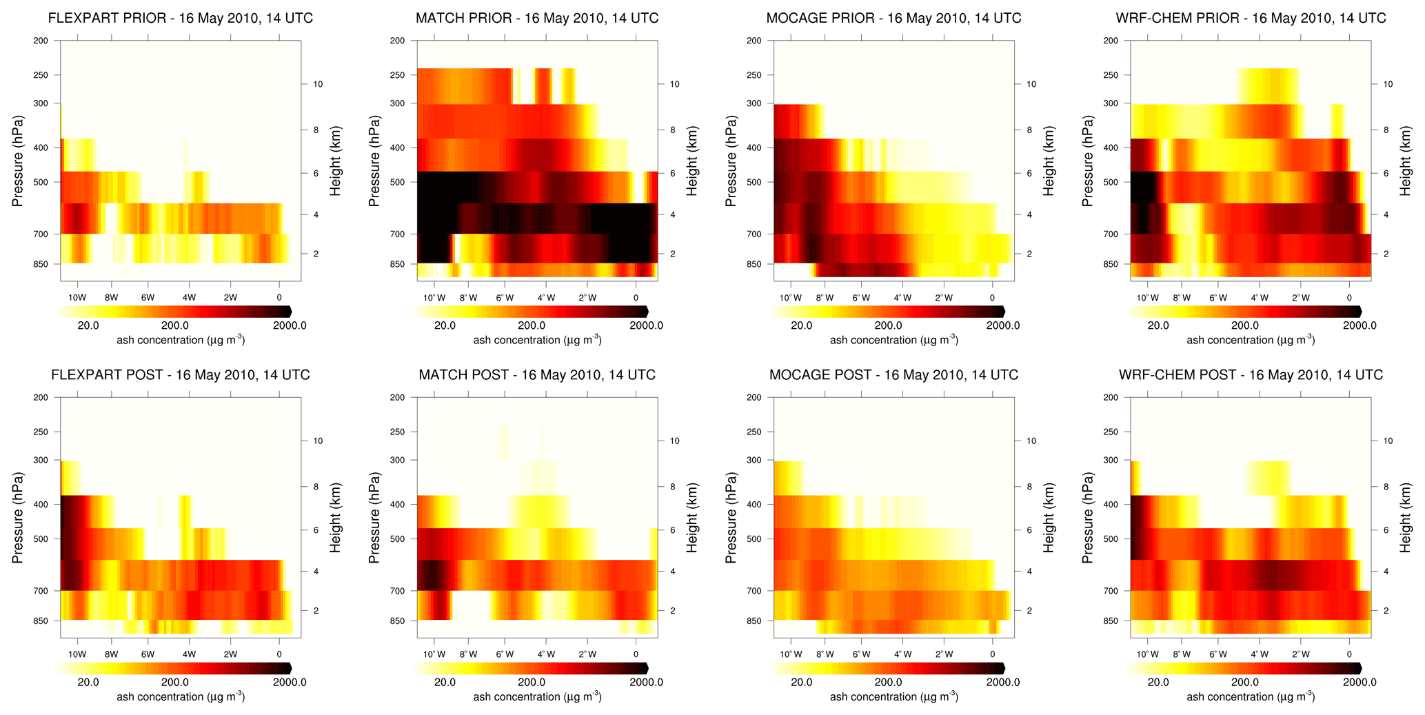
Figure 6 Ash mass concentrations on 16 May 2010 at 14:00 UTC for the four models (from left to right: FLEXPART, MATCH, MOCAGE, and WRF-Chem) with a priori source terms (top) and with a best-estimate a posteriori source term (bottom) across the horizontal line shown in Fig. 5.

While all simulations show ash reaching the ground, the Marenco et al. (2011) airborne measurements, at the same time and in the same area, identified an ash layer only between 4 and 6 km, above the United Kingdom, which corresponds to approximately 5^∘ W to 0^∘ longitude in Fig. 6. This behaviour is also supported by cross sections shown in the Supplement.

The presence of ash at all levels can be due to the source term or due to the representation of vertical processes in the models, and it is possible to provide arguments to help disentangle the two. For most of the source terms, except the MOCAGE a priori one, ash is injected at all layers, and the umbrella-shaped source terms of MATCH and WRF-Chem also tend to emit more ash in the upper levels (Fig. 1). Since the simulated ash by these models tends to extend largely along the vertical (Fig. 6), vertical parameterizations and processes including grid-scale vertical velocity, diffusion, aerosol sedimentation, and/or vertical resolution should probably be improved. Consequently, from this study alone, it is not possible to conclude whether the a posteriori source term is too diluted along the vertical or not.

4 Building ensembles and evaluating their quality

Ensemble forecasting has a 30-year-long history in meteorology (Buizza, 2019), from which some guidelines and pitfalls can be learned for an extension to volcanic ash dispersion forecasting. The first lesson learned is that all possible sources of uncertainty should be taken into account. The possible methods to take into account the uncertainty (perturbations or stochastic representation of features) can be diverse and have been an active field of research (Leutbecher et al., 2017). Another lesson learned is that the evaluation of ensembles is critical and is usually done based on long-period data sets for which homogeneous ensembles are run and compared against measurements. Usually, the evaluation metrics are used to further design the perturbation methods or bounds. Regarding rare events such as volcanic eruptions, for which observations are rare, evaluation of ensembles is clearly a more difficult task.

4.1 Method

Uniform grids facilitate the computation of the ensemble and the ingestion of model products into flight planning software (Hirtl et al., 2020). From the outputs of the four models on the same grid, mini-ensembles were computed. Ensembles in general provide probabilities of a model variable of interest, which is the ash mass in our present application. Based on the meteorological literature (Fundel et al., 2019), there are different ways to present and use ensemble outputs, which depend on the user requirements. In the EUNADICS-AV project, it has been argued that ash concentration maps at several flight levels are important as they can be used in the flight planning software. This allows for the computation of ash dose along flight tracks including its uncertainty by taking into account different levels of probability. Furthermore, flight rerouting should be enabled in highly contaminated regions. So, the choice for this study has been to present the ensemble outputs as maps of ensemble quantiles, including the median (Q50), the 75th percentile (Q75), and the 99th percentile (Q99) of the concentration of ash at every grid point. These three concentration fields at all vertical levels can be used and treated by flight planning software, with different levels of risks.

Based on the different model simulations that were compared in the previous sections, two multi-model ensembles were built:

• a four-member a priori ensemble, based on the four model simulations (FLEXPART, MATCH, MOCAGE, and WRF-Chem) with their own a priori source terms, and

• a 12-member a posteriori ensemble, based on the four models (FLEXPART, MATCH, MOCAGE, and WRF-Chem) using the a posteriori source term, its lower bound, and its upper bound (three simulations per model).

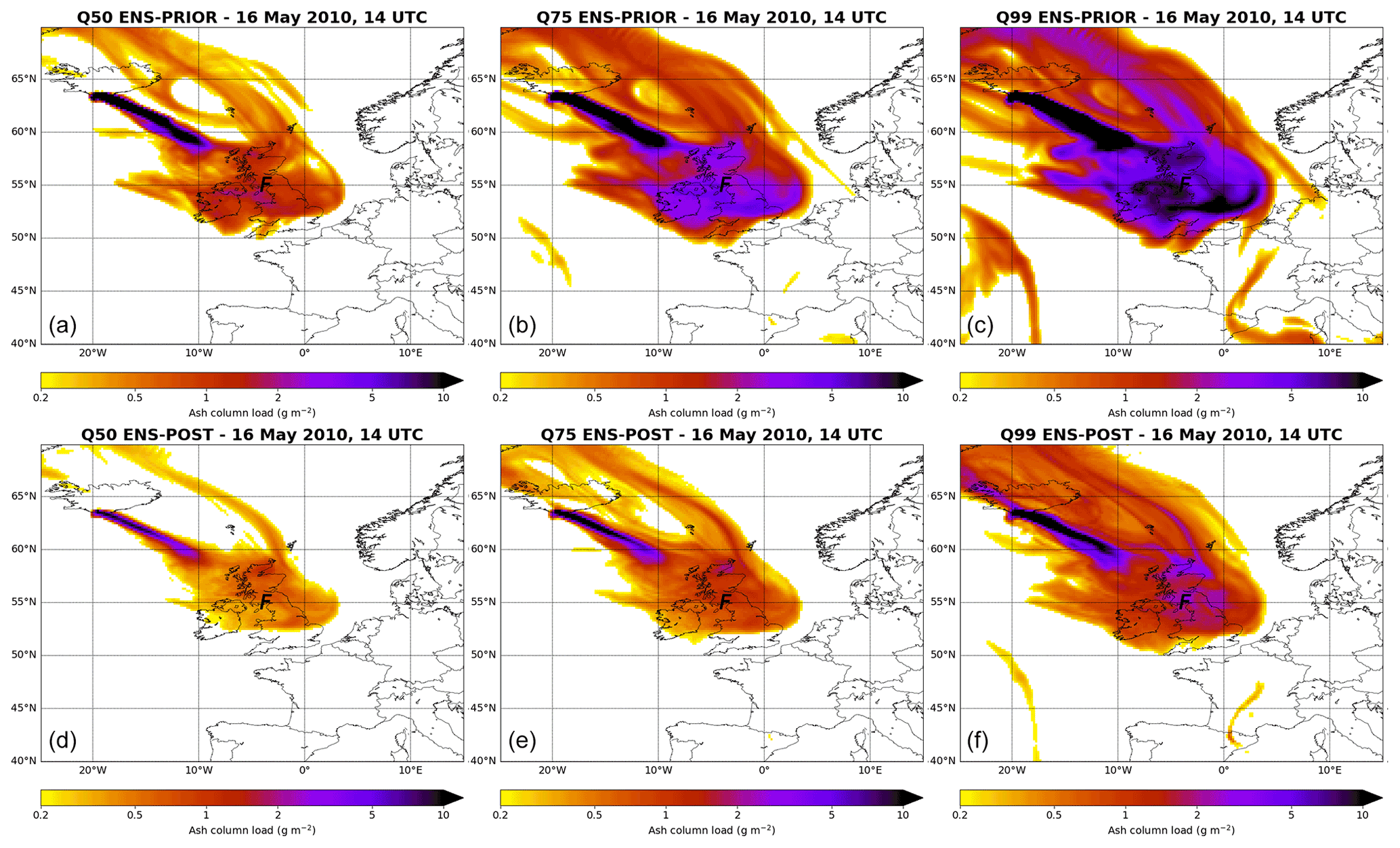
Figure 7 Ash column load on 16 May at 14:00 UTC for the a priori (a–c) and for the a posteriori (d–f) ensembles. The ensemble median (Q50), 75th percentile (Q75), and 99th percentile (Q99) are respectively displayed from left to right.

Figure 7 shows ash column load of the a priori and a posteriori ensembles on 16 May at 14:00 UTC. For both ensembles, differences between the median and Q99 are obvious, which clearly reveals the benefit of the ensemble approach. The differences between the a priori and a posteriori ensemble are also quite large.

Evaluation of ensemble performance is done against VACOS ash location to assess the horizontal spread and against aircraft observations of lidar and in situ measurements in order to evaluate simulated local ash load and ash concentrations along flight routes.

4.2 Evaluation of ash location

Like for the individual model outputs, ash location of ensemble outputs is evaluated using the FSS metric applied to a smaller domain shown in Fig. 3 at 0.2^∘ resolution. While the FSS can differ significantly from one model to another (Fig. 4), the FSSs of ensemble quantiles (Fig. 8) are quite close to each other, except for some specific points in time. In that case, FSSs of the median are higher than the Q99 FSSs. In general, the a posteriori ensemble median performs better than the a priori ensemble median. This is also generally true for the higher quantiles, except for Q99 on 17 and 18 May, when the Q99 quantiles of the a posteriori ensemble show lower performance than the a priori one. However, the differences are rather small. A possible explanation is that in the Q99 a posteriori ensemble (Fig. S6 in the Supplement) the highest values of ash load are not located north of the Netherlands on 17 May (Fig. 3) but to the west of Norway and to the east of Iceland.

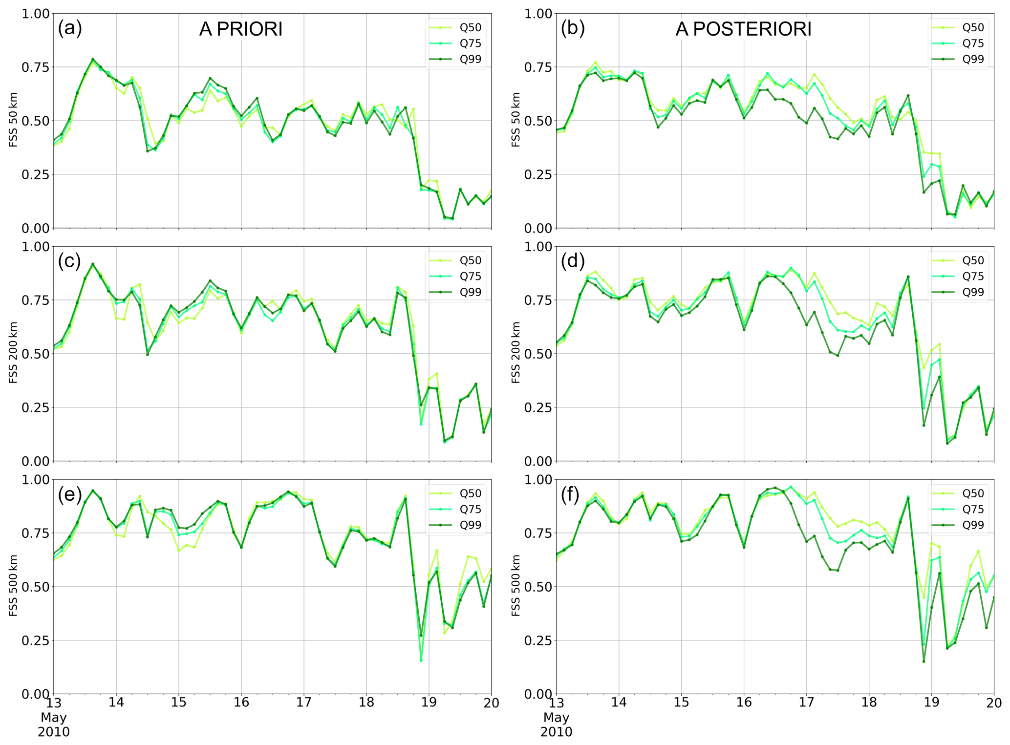
Figure 8 Comparison of the fraction skill score (FSS) of ash column locations, for the ensemble quantile median (Q50), 75th percentile (Q75), and 99th percentile (Q99) with a priori source terms (a, c, e) and with a posteriori source terms (b, d, f). The FSS values are shown for radii of 50 (a, b), 200 (c, d), and 500 km (e, f).

To summarize the capacity of ensemble quantiles to catch the regions of highest ash load, the different ensemble quantiles have similar performance, and the a posteriori ensemble generally performs better than the a priori ensemble.

4.3 Evaluation of ash column load

Evaluation of ash column load is done against the most precise airborne lidar measurements from Marenco et al. (2011). Figure 9 summarizes how the ensemble performs at different points along three flight tracks: on 14 May around 15:00 UTC, on 16 May around 14:00 UTC, and on 17 May around 16:00 UTC. The whole flight track is not taken into account; rather, only some locations (referred to as F in Fig. 7), which correspond to points where the highest values of ash load were measured, are considered. For comparison, ensemble results are extracted from the few (four to nine) grid points obtained along the flight track where those highest values were measured. VACOS data extracted at the same grid points are also superimposed. Although such evaluation does not provide a rigorous probabilistic evaluation of the ensemble, it helps to characterize the ensemble dispersion and shows how the ensemble quantiles match the observations.

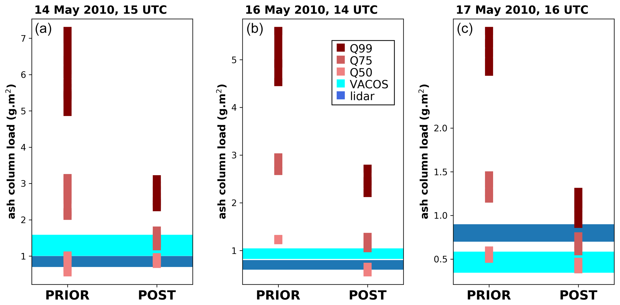
Figure 9 Comparison of ash load (vertical axis, unit g m⁻²), for the a priori (PRIOR) and a posteriori (POST) ensembles (abscissa), at the location of lidar measurements shown in Fig. 3, on 14 May at 15:00 UTC (a), on 16 May at 14:00 UTC (b), and on 17 May at 16:00 UTC (c). The range of lidar, or VACOS, estimates along the flight track are plotted as blue, or light blue, horizontal rectangles. Note that, in these cases, lidar and VACOS values do not overlap. The different quantiles (Q50, Q75, Q99) are plotted as different red tones: the darker the colour, the higher the quantiles. For all data, the values of several grid points are plotted that sample the column loads along the flight track. Note the different y-axis scales.

For the three episodes (Fig. 9), the airborne measurements fall in the range of the median, Q75, or Q99 ensemble values, which shows that both ensembles capture the real ash load. The range from the median to Q99 is smaller for the a posteriori ensemble than for the a priori ensemble: the ensemble dispersion is smaller using the a posteriori source term, though keeping it large enough. The median of the a posteriori ensemble generally fits the range of measured values, except that it is biased low on 17 May at 16:00 UTC. Of course, further calibration based on different test cases should be done to validate these results.

4.4 Evaluation of 3D concentrations

The evaluation of ash concentration is performed against DLR and FAAM aircraft measurements taken during their flight routes. In situ ash measurements are rare, though some exist, particularly for the phase of the eruption studied in the present article. Table 2 compares in situ airborne measurements with ensemble values (using the a priori and a posteriori source terms). The maps of concentration values for different ensemble quantiles and the flight locations are shown in Fig. 10.

Table 2 Ash concentrations reported by DLR (Schumann et al., 2011) and FAAM (Marenco et al., 2011) flights and estimates from the ensemble outputs. The flight level (in brackets) indicates the mid-level of the ensemble output layers closest to the actual flight track heights (from FL25 to FL625 by 50). The concentration measurements are expressed as a range of values (m_min to m_max) for DLR flights or as mean value and uncertainty (m_mean±σ) for FAAM flights.

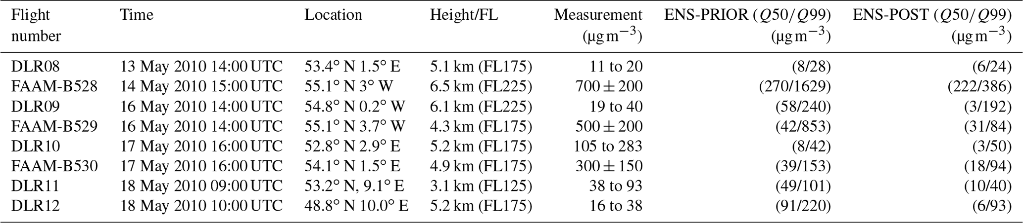
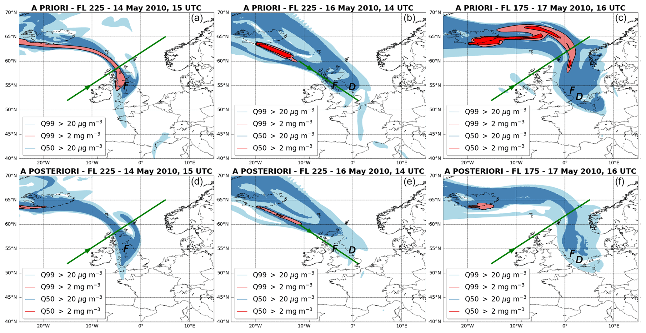
Figure 10 Ash concentrations from the a priori (a–c) and a posteriori (d–f) ensemble, at dates and levels where in situ measurements are available (from left to right: FL225 on 14 May at 15:00 UTC, FL225 on 16 May at 14:00 UTC, and FL175 on 17 May at 16:00 UTC). Blue areas indicate ash concentrations higher than 20 µg m⁻³, with different colour tones for Q50 and Q99. Red colours refer to concentrations above 2 mg m⁻³, with different colour tones for Q50 and Q99. Aeroplane locations are indicated by the symbols F and D, for FAAM and DLR flights, respectively. The green lines refer to the cross sections shown in Fig. 11.

A general conclusion based on Table 2 is that the ash Q99 values based on the a priori source term are much higher than based on the a posteriori source term. This is consistent with the fact that the a priori member with maximum ash concentration yields generally higher values than the a posteriori member with maximum ash concentration (Figs. 5 and 9). On 13 May at 14:00 UTC (map not shown), the ash concentrations are low (around 10 to 20 µg m⁻³), according to the measurements, but also in the ensemble, which is in good agreement for both source terms. On 14 May, the aircraft flew through a rather ash-loaded area (between 500 and 900 µg m⁻³), which is also obviously polluted by ash according to the ensemble, as shown by the corresponding map (Fig. 10). At this time, the a priori ensemble gives a very large dispersion, and the a posteriori ensemble underestimates the ash concentrations.

However, where high ash concentrations are measured (above 200 µg m⁻³), the ensemble values generally tend to be lower. Even for the flight routes where modelled ash column loads are in reasonable agreement with the measurements (FAAM flights, Fig. 9), ash concentrations at the flight levels are significantly lower. An explanation, consistent with conclusions in previous parts of this article, is that ash is too diluted along the vertical, due to the shape of the source term or to vertical dilution processes during ash transport. This is also true for the a posteriori source term which is constrained by ash load satellite estimates, but where the vertical distribution of ash is mainly constrained by the a priori. In general, the a priori ensemble has a large dispersion compared to the a posteriori ensemble.

5 Discussion: use of ensembles for flight planning

Given the threat of ash for flight safety and given the uncertainty of ash dispersion forecasts, the use of probabilistic products is important but not straightforward. The ICAO (2016) plan and latest versions thereof say that the airlines are those that choose how to address the volcanic ash hazard, provided they have their safety risk assessment for operations in the presence of volcanic ash accepted by the appropriate authority. Prata et al. (2019) introduced a risk-matrix approach that combines ash concentration and ash dosage (accumulated ash concentration along the flight route) with likelihood obtained from the ensemble uncertainty. Their ensemble was based on one model with different model parameters, source terms, and meteorology. It was evaluated based on a synthetic hypothetical use case.

In this study on a real case, we found considerable differences in ash location and ash concentrations due to the model choice, indicating that a multi-model ensemble increases information about uncertainty. Even though the a posteriori ensemble was, in general, in better agreement with the observations, an a priori ensemble is preferred for flight planning as it is also available in near-real time during the early phase of an eruption. The a posteriori source term can only be computed if a sufficient number of measurements are available. Due to the limited number of ground-based measurements, the missing temporal coverage of measurements from polar-orbiting satellites, and only a few instruments on geostationary satellites, it usually takes a couple of hours to days to gather sufficient high-quality ash measurements to compute the a posteriori source term. Thus, a better quality of past ash dispersion and therefore better initial conditions for upcoming ash forecasts can only be obtained after several hours or even a few days. An a priori ensemble includes different realizations of the source term, the most important component of ash dispersion uncertainty. The wide range of these a priori ash dispersion forecasts, however, might result in too conservative of flight planning, which can only be eased when a refined a posteriori source term is available. An intermediate approach could be to update the a priori source term continuously by constraining the assumptions of the source term evolution with updated measurements, or plume height estimates for instance.

The evaluation of both ensembles revealed that ash location and load are in good agreement with the observations. However, the vertical structure of ash clouds is not correctly represented by the models, and ash concentrations at individual flight levels are biased low. Therefore, care must be taken concerning flight rerouting. Flying between distinct layers of ash would only be possible knowing the precise vertical structure of ash clouds, which is clearly not the case. However, the models provide useful guidance in the sense that flying above the predicted clouds and also around highly contaminated regions may be possible.

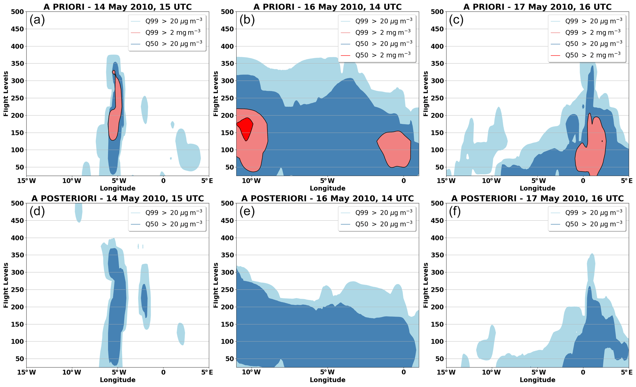
Ash concentrations smaller than 2 mg m⁻³ are considered safe. Ash concentrations higher than 80 mg m⁻³ are definitely considered unsafe (Clarkson et al., 2016). Following a conservative approach, we therefore recommend avoiding regions within the 2 mg m⁻³ contour line of the Q99 of the a priori ensemble. Looking at Fig. 10, such no-fly areas would include a thin plume from Iceland to the United Kingdom on 14 May, a small band south-east of Iceland on 16 May, and a larger band which spreads from the east of Iceland along the 65^∘ latitude towards the North Sea on 17 May. The days 16 and 17 May were the most severely affected by flight cancellations during the considered time period of this study, when 20 % and 31 % of all flights were cancelled in Ireland and 19 % and 26 % in the UK (EUROCONTROL, 2010). Knowing that the vertical distribution of ash is not correctly represented in the models, vertical cross sections can nevertheless be used to estimate the upper height limit of the ash cloud. The cross sections shown in Fig. 11 reveal high ash concentration on 14, 16, and 17 May at different vertical levels for the a priori ensemble. Such hazardous regions are not obvious in the a posteriori ensemble. Considering the entire 3D field of ash concentration and using an appropriate flight planning software (Rokitansky et al., 2019; Hirtl et al., 2020) would help to avoid these regions.

Figure 11 Ash concentrations from the a priori (a–c) and a posteriori (d–f) ensemble along the cross sections shown in Fig. 10. The dates and the colour legend are the same as in Fig. 10.

Flight cancellations can therefore be avoided by flying through lower contaminated regions as demonstrated during the EUNADICS-AV exercise (Hirtl et al., 2020). Maintenance intervals of individual aircraft can then be obtained with flight planning software accumulating ash dose along relevant flight routes. In a later perspective, the quantiles can be used to optimize the cost $/$ loss function, in a similar approach as the one developed by other end-users of meteorological ensemble forecasting (Richardson, 2000).

This approach would lead to better management during future volcanic eruption crises. Probabilistic ash concentration forecasts, combined with certain “no-fly” areas, could become the future operational ash products, enabling safety as well as cost considerations of flying in the presence of such hazards. This would result in much less impact caused by flight cancellations and a reduced number of reroutings and traffic flow congestion during volcanic ash events.

6 Summary and conclusions

This article has presented an inter-comparison of volcanic ash forecasts using different models and different source terms for the Eyjafjallajökull eruption in May 2010. Furthermore, a methodology to build and use an ensemble for ATM and flight planning was discussed. Most important findings include the following.

• Large differences in ash location and ash load were found when models were run with their individual a priori source terms, which confirms that ash dispersion forecasts are highly sensitive to the volcanic ash source term.

• An a posteriori source term together with its perturbation can be shared and used as input for any model, yielding a multi-model ensemble; this a posteriori ensemble performs satisfactorily for ash location in two dimensions and for ash column load.

• The main shortcoming of all simulations is the vertical representation of ash concentration, which is evenly distributed over a wide vertical range without distinct layers of ash. Therefore, the vertical distribution of ash would need to be improved in relation to the source term – even after inversion – but also as a consequence of vertical aerosol processes in models (sedimentation, diffusion, aggregation). Even with a vertically layered source term, there is high vertical diffusion of concentrations some hours after the emission.

• Quantiles of concentrations are relevant products for ATM. They can be used for route optimization in the areas where ash does not pose a direct and urgent threat to aviation. Probabilistic ash concentration forecasts combined with safe “no-fly” areas can become a future operational product for ATM.

• The a priori ensemble is also available in near-real time in the early phase of an eruption, but the wide range of areas affected by ash dispersion will in most cases lead to very conservative flight planning. This behaviour might be case-dependent, although experience shows that a priori source terms rather overestimate ash emissions. Therefore, flight rerouting can be based first on an a priori ensemble, and only at a later stage, when the a posteriori ensemble is available, can less conservative approaches be taken for flying through low-concentration ash clouds.

In this study, only source term and model process uncertainty have been taken into account. In real conditions, the meteorological forecast error cannot be neglected and would also increase the spread in plume location and ash column loads.

A rigorous evaluation of any ensemble should be done for a large number of cases, which is difficult for rare events such as volcanic eruptions. In addition, few measurements are available, hindering a comprehensive ensemble evaluation. The use of observations by assimilation along the vertical (such as lidar data) could improve the model and ensemble representation of ash, even though such measurements remain rare and are available only where the ash plume is thin enough to be penetrated by the lidar.

The proposed methodology cannot only be applied for ash dispersion during volcanic eruptions but also for other air pollutants, such as SO₂, desert dust, or forest fires. Every airspace closure or even rerouting of aeroplanes immediately increases the costs for airlines, so they could introduce in their risk management plan some acceptance to fly at least through regions which are below the safety-critical pollutant concentration threshold. For future natural disasters, cost and disruption of air traffic could be eliminated to a great extent by including the results of dispersion models into flight planning software to apply cost-based trajectory optimizations.