the Creative Commons Attribution 4.0 License.
the Creative Commons Attribution 4.0 License.
 | 20 Aug 2021
Quantifying location error to define uncertainty in volcanic mass flow hazard simulations
Jonathan Procter
Gabor Kereszturi
The use of mass flow simulations in volcanic hazard zonation and mapping is often limited by model complexity (i.e. uncertainty in correct values of model parameters), a lack of model uncertainty quantification, and limited approaches to incorporate this uncertainty into hazard maps. When quantified, mass flow simulation errors are typically evaluated on a pixel-pair basis, using the difference between simulated and observed (“actual”) map-cell values to evaluate the performance of a model. However, these comparisons conflate location and quantification errors, neglecting possible spatial autocorrelation of evaluated errors. As a result, model performance assessments typically yield moderate accuracy values. In this paper, similarly moderate accuracy values were found in a performance assessment of three depth-averaged numerical models using the 2012 debris avalanche from the Upper Te Maari crater, Tongariro Volcano, as a benchmark. To provide a fairer assessment of performance and evaluate spatial covariance of errors, we use a fuzzy set approach to indicate the proximity of similarly valued map cells. This “fuzzification” of simulated results yields improvements in targeted performance metrics relative to a length scale parameter at the expense of decreases in opposing metrics (e.g. fewer false negatives result in more false positives) and a reduction in resolution. The use of this approach to generate hazard zones incorporating the identified uncertainty and associated trade-offs is demonstrated and indicates a potential use for informed stakeholders by reducing the complexity of uncertainty estimation and supporting decision-making from simulated data.
- Article
(18248 KB) - Full-text XML
- BibTeX
- EndNote


Mass flow numerical models are frequently used to predict the hazard from future events (e.g. Procter et al., 2010b; Scott et al., 1997, 2005; Aguilera et al., 2004; Pistolesi et al., 2014; Darnell et al., 2013; Thouret et al., 2013), understand fundamental processes within mass flows, investigate previous events (e.g. Iverson and George, 2016), and determine impacts to elements exposed to the flow (e.g. Zeng et al., 2015; Mead et al., 2017). Their utility and advancing computational power have positioned numerical models, of various scales and complexity, as a critical risk management and decision-making tool (Bennett et al., 2013). An important element of risk management and decision-making in a natural hazard context is the quantification and communication of uncertainty (Thompson et al., 2015; Doyle et al., 2014). In numerical modelling, much uncertainty is associated with a model's predictive accuracy in which inaccuracies can stem from input and boundary conditions, model assumptions, and numerical limitations. However, testing model accuracy, eliciting the effect of inputs, assumptions, and limitations on accuracy, and communicating these effects is a non-trivial task (Bennett et al., 2013; Jakeman et al., 2006; Wealands et al., 2005; McDougall, 2016).
The fundamental requirement for assessing model accuracy is the establishment of a baseline, “true”, dataset for comparison between model and reality. Experimental facilities and studies (e.g. Iverson et al., 2010; Lube et al., 2015) can provide detailed observations of mass flow processes to validate, develop, and benchmark numerical models. Some known, important processes (e.g. initial conditions, unconfined flow, interaction with topography) are simplified in these facilities, and an assessment of “subsystem” model accuracy (using definitions of Esposti Ongaro et al., 2020; Oberkampf and Trucano, 2002) requires the application to “real world” mass flow observations. However, such measurements of mass flow characteristics are mostly limited to post hoc analyses of events in which data are derived from static (i.e. single points of data not varying in time) observations such as deposit depth, flow outlines, and flow height markers (Charbonnier et al., 2013, 2017; Procter et al., 2014). Temporally varying measurements of mass flows do exist, for example, when the occurrence is known a priori (e.g. in Procter et al., 2010a) or when permanent sensors (e.g. seismometers) capture some aspect of the flow (Coviello et al., 2018; Walsh et al., 2016). While these direct observations can provide benchmarking opportunities for mass flow models, they are rare and currently not comprehensive enough to quantify the entire range of mass flow sizes and behaviours. Therefore, performance measurement will predominantly need to utilise static, post hoc observations.
In general, quantifications of model performance can be split into global or local comparisons (Wealands et al., 2005). Global comparisons characterise a mass flow into single, easy to interpret metrics (e.g. length of flow, area inundated; Charbonnier et al., 2017; Mergili et al., 2017) but can disguise both spatial and temporal divergent behaviour (Bennett et al., 2013). Local comparisons of model performance typically utilise a confusion matrix (Bennett et al., 2013; Charbonnier et al., 2017; Mergili et al., 2017) to classify proportions of correctly or incorrectly simulated data points, in which spatial accuracy of simulators can be evaluated by comparing pixel pairs on a map (Wealands et al., 2005). However, there is no universal metric for quality (Bennett et al., 2013), and various measures can be used depending on objectives or potential uses of the simulator (Bennett et al., 2013; Jakeman et al., 2006). Pixel-pair comparisons are also prone to registration issues (e.g. when systematic errors in base data or observations shift results; Wealands et al., 2005; Koch et al., 2015; Foody, 2002) that, even if small, can decrease overall accuracy metrics (see, for example, Charbonnier et al., 2017) due to the lack of tolerance for spatially or quantitatively minor errors. The conflation of quantity and spatial errors is particularly relevant for mass flow models, in which the likelihood of errors generally decreases as flow depths increase.
The conflation of these scale and location errors and reliance on precise co-location in comparisons contrast with human (i.e. qualitative) comparisons that provide for some error tolerance and, through focusing on basic spatial structure, logical coherence and importance-weighting of similarities (Hagen, 2003; Koch et al., 2015; Wealands et al., 2005). Human visual comparison is a powerful method for comparing and evaluating spatial field results (Wealands et al., 2005), and many comparison approaches attempt to emulate the human ability to distinguish between residual or random errors and errors in registration (i.e. account for co-location errors) and resolution (i.e. account for errors that are only significant at certain scales; Costanza, 1989). These approaches, identified and reviewed in Wealands et al. (2005), include multi-resolution comparisons (Costanza, 1989) to identify similarity of measurements with scale; region clustering, segmentation, and homogenisation to identify and compare patterns in the spatial field; importance weighting to focus performance evaluation on the most (hydrologically) important regions; and fuzzy comparisons to represent relative membership (“fuzziness”) of each map cell to a certain category (e.g. inundated/not inundated). Despite this range of potential performance evaluation methods, there is no universal criterion or method to evaluate model quality (Bennett et al., 2013), and there are few examples of mass flow model performance evaluations that identify the level of both location and quantification error.
Robust, objective, and complete evaluations of model performance that quantify the uncertainty of predictions and effect of model and input parameters are essential for the development and use of mass flow models as a reliable hazard forecasting tool (McDougall, 2016; Calder et al., 2015). The selection of input parameters and modelling approach can be achieved through calibration (often visual; McDougall, 2016); however, this limits a quantitative elicitation of the effect model and input parameter choices have on the hazard prediction. Appropriate model performance evaluation would not only quantify this uncertainty but also communicate the scale and spatial dependence of these effects, presenting opportunities for new hazard delineation methodologies. This paper presents a performance evaluation approach using a multi-scale fuzzy comparison technique that incorporates positional error tolerance to assess debris flow model performance. The 2012 debris flow from the Upper Te Maari crater, Tongariro volcanic centre (New Zealand), is used as a benchmark to test the effect of debris flow model choice on simulation accuracy. Given the necessity to assess model performance on the basis of its constructed purpose (Jakeman et al., 2006), each model is evaluated in terms of its ability to delineate hazardous debris avalanche inundation zones, and this demonstrates a new approach to define these zones with quantified uncertainty.
The 6 August 2012 eruption in the Tongariro volcanic centre was a short (<60 s) but complex eruption sequence beginning with a slope failure on the outer, western flank of the Upper Te Maari Crater, followed by a series of (in order) eastward, westward, and vertically directed blasts that generated pyroclastic surges and ballistics covering an area greater than 6 km2 (Jolly et al., 2014; Lube et al., 2014; Procter et al., 2014; Fournier and Jolly, 2014). The Te Maari debris avalanche emplacement, morphology, and deposit characteristics were identified and summarised in Procter et al. (2014); here we summarise only the necessary details for this study.
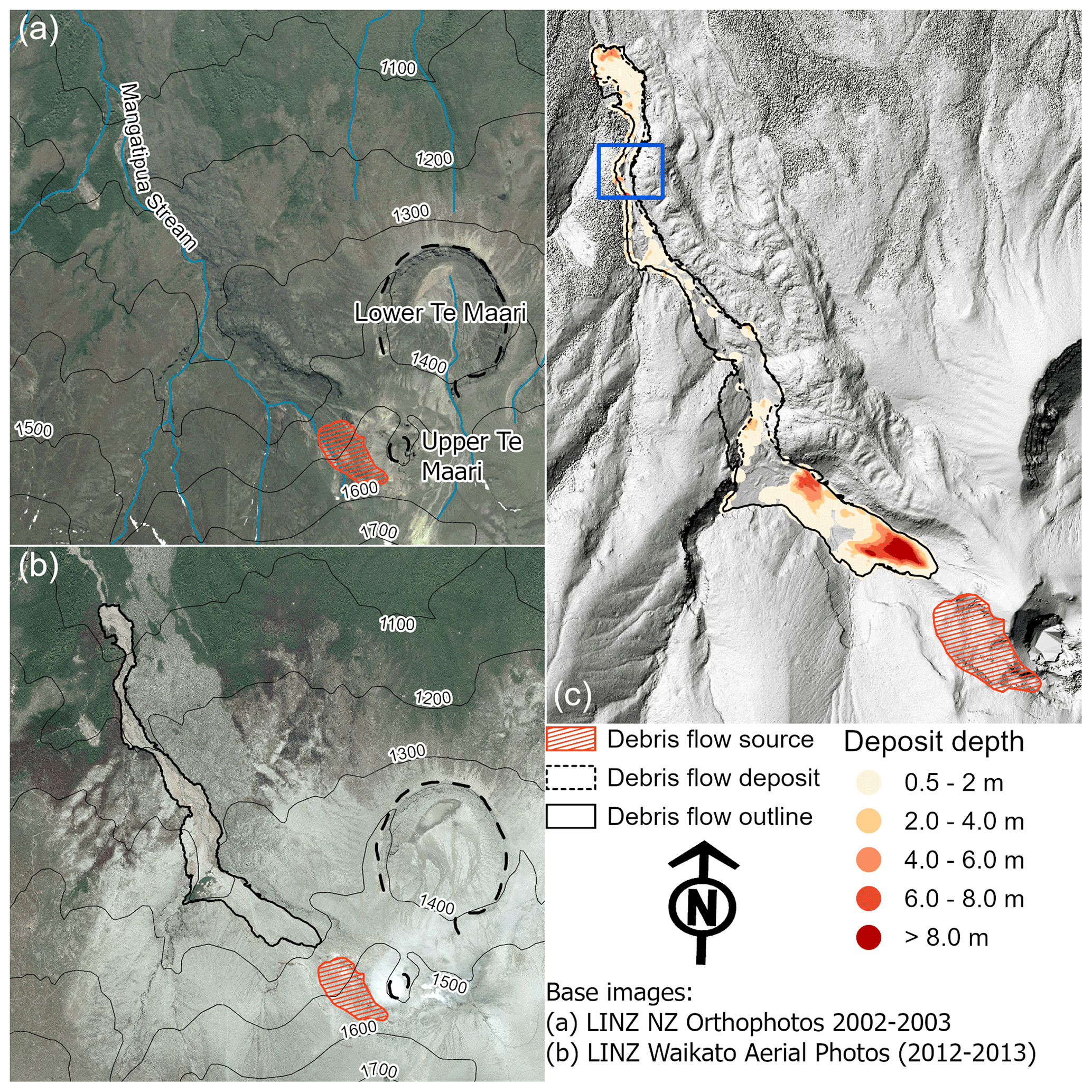
Figure 1Te Maari debris avalanche case study region (a) pre-eruption, (b) post-eruption, and (c) debris avalanche deposit depth and outline. The blue rectangle in (c) shows area of spurious elevations from source digital terrain model.
The debris avalanche generated from the slope failure is presumed to have begun at 11:49:06 UTC, which is when an earthquake located at the avalanche head scarp is detected in the seismic record by Jolly et al. (2014). The cohesive, clay-rich debris avalanche was mostly confined by the Mangatipua Stream, travelling downslope to reach a run-out of approximately 2 km (Lube et al., 2014; Procter et al., 2014; Walsh et al., 2016). Volume of the debris avalanche was estimated between 6.83 and 7.74×10⁵ m3 in Procter et al. (2014), measured as the difference between a 10 m pre-event digital terrain model (DTM) and post-event lidar-derived DTM. The mud–sand matrix-supported debris flow deposits were primarily emplaced in four lobes along Mangatipua Stream (see Fig. 1). Coarse, poorly sorted clasts ranging in size from pebbles to large boulders were also present, particularly at frontal lobes and lateral margins of the deposit, generally decreasing in quantity downstream. Between the lobes, steep channel sides limited deposition with 1 to 2 m of erosion into the soil substrate and thin (0.2 to 0.5 m) veneer deposits, demarcating maximum extents of the flow.
Geomorphic change associated with the debris flow was calculated through comparisons between the 10 m pre- and post-event lidar-derived DTMs. The pre-event DTM was created from contours generated from stereo-photogrammetry captured in 1975, with an accuracy of 90 % within 10 m. The lidar post-event DTM was acquired on 8–9 November 2012 and has a 1σ accuracy of 0.25 m horizontally and 0.15 m vertically. While the accuracy of both terrain models is within acceptable limits, there are a number of issues in terrain model interpolation, representation, and acquisition time, which limits the comparison between terrain models and usage in numerical modelling. Interpolation of contours to generate the pre-event DTM results in a smoothed representation of terrain with no sharp gradients, which results in an inaccurate representation of steep features and narrow sections of Mangatipua Stream (Procter et al., 2014). One major zone of misrepresentation is in the upper section of lobe 4, highlighted in Fig. 1. In this region, elevation of the pre-event DTM increases to form a barrier to flow along Mangatipua Stream which is not present in the field. The magnitude of this error is unknown, but the height difference between pre- and post-event DTMs indicate it could be between 10 and 15 m. Additionally, the lidar survey used to generate the post-event DTM was taken 3 months after the debris flow and almost 1 month after a breakout lahar (13 October 2012, Walsh et al., 2016) caused through damming of Mangatipua Stream by the initial debris avalanche (Walsh et al., 2016; Procter et al., 2014). The breakout lahar, and possibly subsequent streamflow, eroded and entrained the 6 August debris avalanche and ash deposits, redistributing sediment further downstream and cutting a new stream into the deposit. Therefore, the post-event DTM does not represent the exact morphology of Mangatipua Stream immediately after the debris flow.
Despite the previously mentioned uncertainties, the difference between the pre- and post-eruption DTMs form a useful dataset for evaluating the accuracy of numerical models. Figure 1c shows the deposit outline (dotted black line) used in the accuracy assessment (see “Model performance assessment” section) and points of deposit depth. Deposit depth points are a subset of deposit depths in Procter et al. (2014) in which the depth estimates are least affected by uncertainties in both terrain models. The points all have depths greater than 0.5 m (i.e. larger than lidar inaccuracies, avoiding veneer deposits) and are located where the pre-event terrain slope is moderate (<15∘) to avoid the effects of smoothing high-gradient slopes in the pre-event DTM. An outline of the debris avalanche, shown as the black line in Fig. 1, was created as the union of the debris avalanche outline in Procter et al. (2014) and outline of the debris avalanche detected using image classifications from an airborne hyperspectral survey in 2016. While this survey was undertaken 4 years after the eruption, thin veneer deposits appear to be detected and classified well (Kereszturi et al., 2018), improving the estimates of flow outline.
3.1 Numerical mass flow models
Numerical techniques to predict the motion of debris avalanches (and debris flows) commonly employ depth-averaging to simulate large-scale geophysical flows (McDougall, 2016; Fischer et al., 2012), being favoured for their computational efficiency (in comparison to three-dimensional models), comparative scales, and level of detail to field measurements (Iverson and Ouyang, 2014). However, the physics of granular and granular-mixture flows is an area of active research, and there are no universally accepted constitutive laws for debris flows (McDougall, 2016). As a result, several models, varying in complexity from single-phase rheologies (e.g. Voellmy–Salm, Christen et al., 2010; O'Brien et al., 1993) to two-fluid (Pitman and Le, 2005) and multiphase approaches (Pudasaini, 2012; George and Iverson, 2014), have been used to simulate debris flows and avalanches (e.g. Iverson and George, 2016; Procter et al., 2010c; Mergili et al., 2017; Iverson et al., 2016; Sosio et al., 2007, 2012; Sheridan et al., 2005).
For all models studied here, the depth-averaged system of equations can be expressed in Cartesian coordinates as follows (Patra et al., 2005; Pudasaini, 2012):
where U is the height and momentum vector, F and G are momentum fluxes in the x and y directions respectively, and S is the source term representing the net driving force (Patra et al., 2005, 2018). The three models in our study utilise different assumptions and simplifications, and all four vectors (U, F, G, and S) vary between models. The models studied here are the Pitman and Le (2005) two-fluid model and Voellmy–Salm rheology model (Salm, 1993; Fischer et al., 2012), both implemented in the Titan2D toolkit (Patra et al., 2005; Pitman et al., 2003), and the Pudasaini (2012) two-phase model, implemented in the avaflow software package (Mergili et al., 2017). The aim of this section is to summarise the features and key differences between each model that may affect model comparison. Readers are referred to the source publications for complete model implementation details and justification of assumptions.
The Voellmy–Salm model (Salm, 1993) is a single-phase rheological approach similar to shallow-water approaches, solved to find the unknown vector , where h is the debris flow depth, and u and v are the depth-averaged x and y direction velocities. The source term in this model assumes a combination of coulomb-like basal friction, proportional to the coefficient μ, and a velocity-dependent turbulent friction, with coefficient ξ (Christen et al., 2010). This combination of friction terms enables the simulation of both high- and low-velocity phases of the debris flow (Christen et al., 2010) but requires calibration of two coefficients (μ, ξ) which may vary depending on topography and material properties (Fischer et al., 2012).
The Pitman and Le (2005) and Pudasaini (2012) approaches approximate the combined motion of granular material and interstitial fluid, solving for the unknown momentum of both components (fluids in Pitman and Le, 2005, and phases in Pudasaini, 2012). In the Pitman and Le (2005) approach, the vector , where φ is the solid volume fraction, and subscripts “s” and “f” indicate the solid and fluid components of velocity. The Pitman and Le (2005) model contains several features (comparted to the Voellmy–Salm model) that may affect the debris avalanche simulations:
- i.
To account for the non-hydrostatic pressure distribution in granular materials (Scheidl et al., 2014), the earth pressure coefficient is used to relate the bed parallel (σl) to bed normal (σn) stresses. The active and passive earth pressures are calculated from the internal (ϕi) and basal (ϕb) frictions (Savage and Hutter, 1989; Pitman and Le, 2005; Iverson, 1997) depending on whether the flow is expanding (accelerating) or contracting (decelerating).
- ii.
Solid (granular) and fluid (water) interaction is accounted for through a Darcy-like drag model and buoyancy effects, which alter energy dissipation within the flow.
This additional detail requires the specification of the volume fraction φ and the granular materials internal (ϕi) and basal (ϕb) friction coefficients.
The Pudasaini (2012) model, in a different formulation to that of Pitman and Le (2005), also accounts for buoyancy effects but also considers the effect of relative motion between fluid and granular phases through a “virtual mass” term C. This parameter and the density ratio are in the vector . While this formulation appears more complex than previous models, this approach still only contains six unknown variables (i.e. as in Pitman and Le, 2005, approach). The most notable differences in regards to debris avalanche simulations are as follows:
- i.
The virtual mass, C, means the solid and fluid components of the debris flow are not assumed to be “interlocked” (relative velocity between phases of 0), and phase separation (such as at deposition) is accounted for, which is a key difference between the Pitman and Le (2005) and Pudasaini (2012) models.
- ii.
The source term contains a buoyancy-modified Coulomb term as in Pitman and Le (2005) and a “generalised drag” term incorporating viscous drag effects. The generalised drag accounts for granular and fluid contributions to drag, the ratio of which depends on the interpolation parameter P with an exponent, J, controlling whether the drag term is linear or quadratic (i.e. similar to Voellmy–Salm models). At P=0 and J=1, the Pitman and Le (2005) drag model is recovered.
The generalised drag term and virtual mass coefficient extends the applicability of the model for all types of granular–fluid flows, including at extremes (i.e. high or low solid fraction flows), but requires the specification of 14 parameters. While many of these parameters can be specified from field/material properties (see, for example, Mergili et al., 2017), some values (e.g. I, P, C) require calibration.
From an application point of view (i.e. neglecting differences in numerical solution techniques), these models vary in their level of description (“completeness”) of debris flow physics. It is important to identify that even well-observed and quantified debris flows, such as the one studied here, may have considerable uncertainty in material properties, which can expand the unknown (i.e. to be calibrated) parameter space. Therefore, while some models may offer more complete descriptions of debris flow physics, there may not be a commensurate improvement in prediction compared to less complex models when uncertainty in material properties is considered. Therefore, this study analyses the performance of all three models to elicit, under locational uncertainty, the relative improvements and trade-offs in accuracy considering calibration and parameterisation needs.
3.2 Initial and boundary conditions
The DTM, location, and height of debris avalanche source material are common inputs to all debris avalanche simulators in this study. The DTM input was defined from the 10 m pre-event terrain model, modified to (a) remove the previously discussed misrepresentation of elevation (see Fig. 1) along Mangatipua Stream and (b) remove the debris avalanche source from the terrain model. The spurious elevation was modified by adjusting elevations in this region to equal the post-event lidar survey elevations. Terrain model elevations in the source area were also adjusted to account for debris avalanche material to be simulated, using source depths from Procter et al. (2014) which were used as the input for the initial pile of debris avalanche material.
The parameters used in each debris avalanche model simulation are shown in Table 1. For the selection, these values were derived from previous examples of debris avalanche simulations in the literature and the authors' experience (e.g. Mergili et al., 2017; Sosio et al., 2012; Mead and Magill, 2017), as well as visual comparisons to flow and deposit properties (i.e. similar to visual calibration in McDougall, 2016). Best-fit values for similar parameters (basal friction and solid volume fraction) in Table 1 vary as a result of the differing drag contributions, parameter sensitivity, rheological and constitutive models, and the calibration approach. For example, the two-phase models only apply basal friction to the solid volume fraction, whereas the (single-phase) Voellmy–Salm approach considers a bulk basal friction of the fluid–solid mixture, and additional viscous stresses in the Pudasaini (2012) model appeared to reduce the sensitivity and value of basal friction. Since the aim of this study is to demonstrate performance evaluation to delineate hazard zones a priori, we chose not to undertake further calibration of parameters (such as in Charbonnier et al., 2017). This best represents typical conditions in which the only data available are flow and deposit outlines.
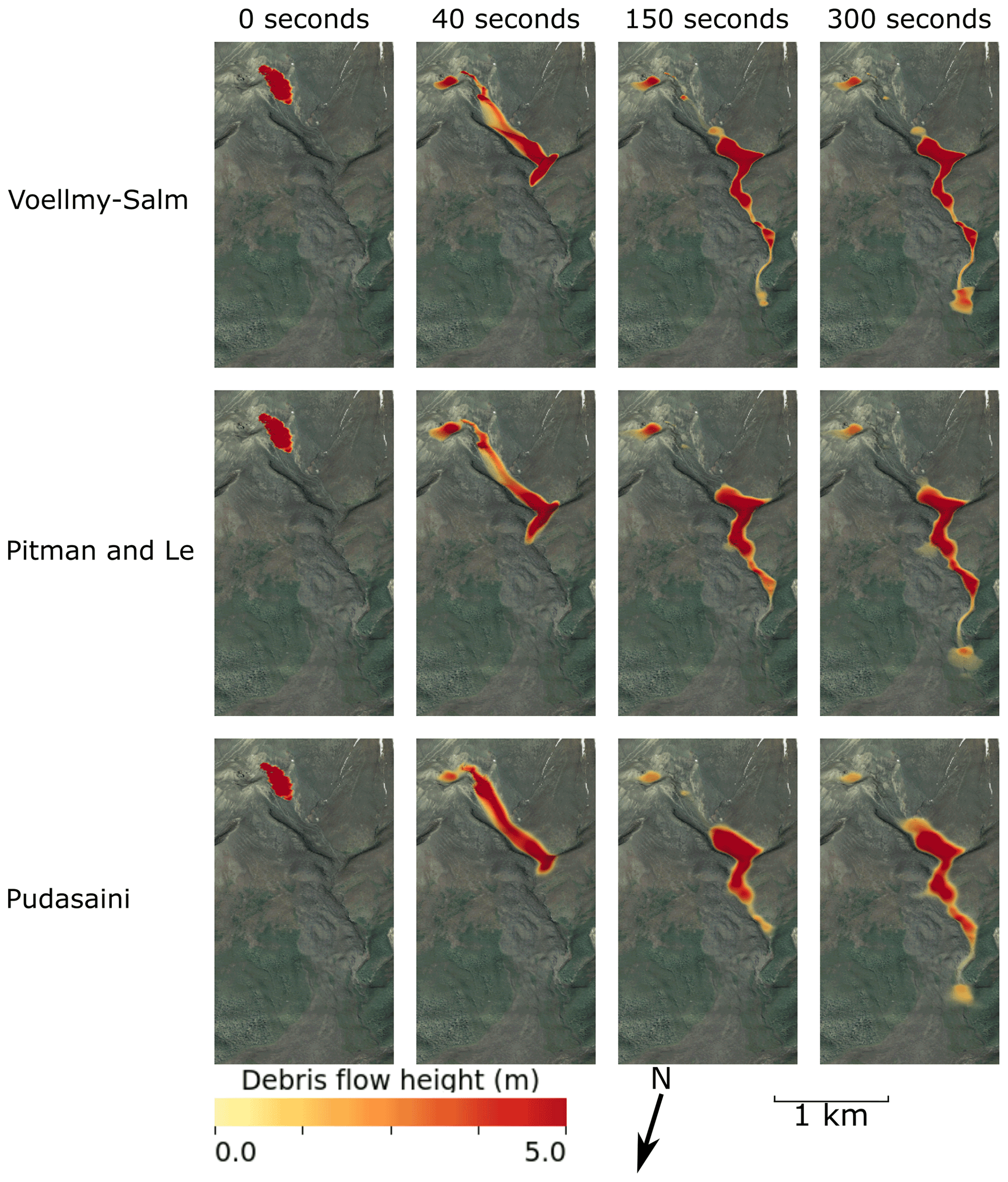
Figure 2Snapshots of simulated debris flow height for each flow model at 0, 40, 150, and 300 s after initiation. Aerial basemap sourced from LINZ Waikato Aerial Photos 2012–2013.
Table 1Debris flow simulation parameter settings for all models.
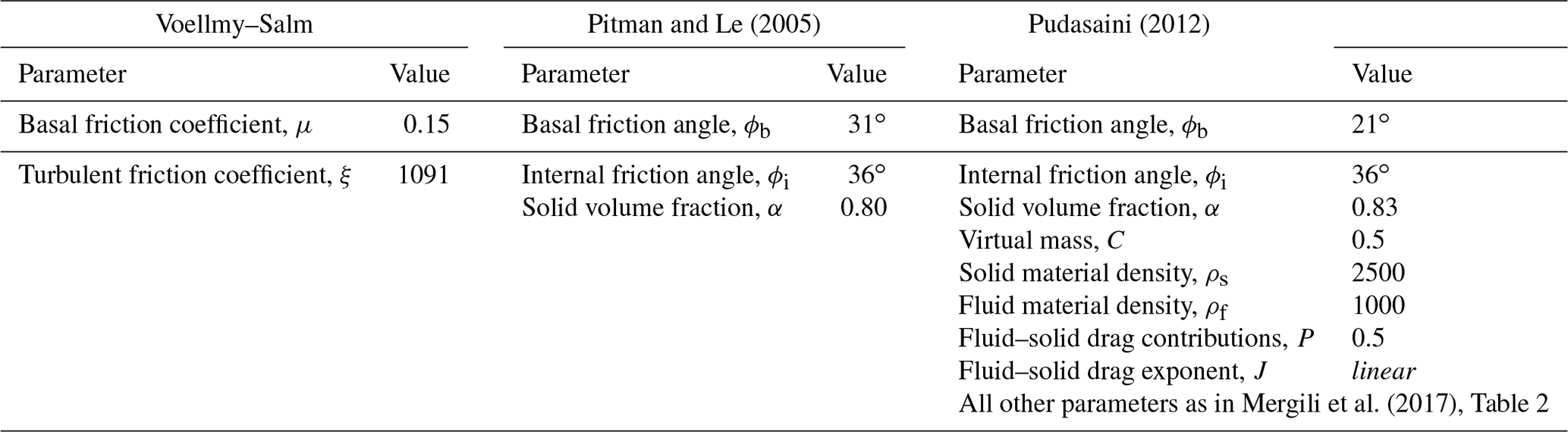
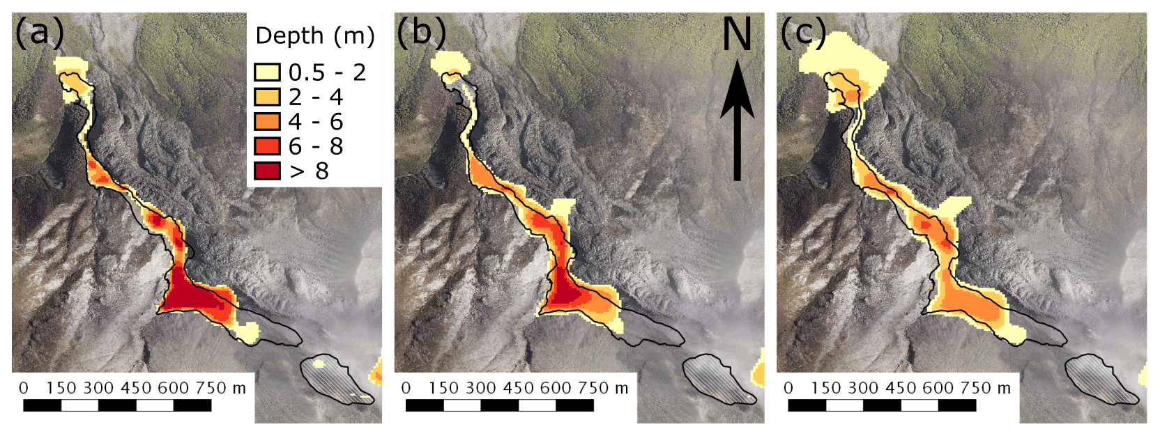
Figure 3Simulated deposit depth for (a) Voellmy–Salm, (b) Pitman and Le (2005), and (c) Pudasaini (2012) models compared with the observed deposit and source outline (black). Aerial basemap sourced from LINZ Waikato Aerial Photos 2012–2013.
3.3 Simulation results
Snapshots of the simulated debris flow depth are shown in Fig. 2 for each model. Simulated debris flow behaviour is generally similar for all three modelling approaches, being an acceleration of material from rest at the debris avalanche source to the upper reaches of Mangatipua Stream (0–40 s) where debris flow material ponded (∼40–100 s, not shown) and gradually travelled downstream to its rest (150–300 s). This is in agreement with field and lidar-based interpretations of the event (Procter et al., 2014), and best-fit volume fraction (0.8–0.85) parameters of the Pitman and Le (2005) and Pudasaini (2012) models support the hypothesis of an unsaturated debris flow. Visual, qualitative comparisons of flow and deposit outlines also appear to match reasonably well to observations. While the Voellmy–Salm simulation shows less ponding in upper Mangatipua Stream and has a more defined (i.e. steeper) distal deposit compared to the other simulations, other differences between simulations appear minor.
Figure 3 shows the simulated deposit depth (at 300 s) for each model. Black lines indicate the observed deposit and source outlines from Procter et al. (2014). Accurate prediction of deposition is difficult in these depth-averaged approaches as none explicitly consider stopping of material (Mergili et al., 2017). The predicted deposit outlines for all simulations appear (qualitatively) to have similar levels of accuracy as other depth-averaged debris flow case studies (e.g. Rickenmann et al., 2006; Iverson and George, 2016; Charbonnier et al., 2017). The most notable difference in simulated deposits is between Voellmy–Salm (i.e. a rheological approach, Fig. 3a) and the two-fluid approaches (Fig. 3b and c). The Voellmy–Salm simulated deposit is mostly confined to the Mangatipua Stream, whereas the two-fluid approaches show more spreading of the distal deposit and shallow flow in areas of super elevation.
The previous qualitative comparisons between field observations and simulation results can provide some credibility to flow predictions; however, modern, robust hazard assessments require quantitative evaluations of model performance to understand the level of uncertainty in model predictions. Previous assessments of flow simulation accuracy (Mergili et al., 2017; Charbonnier et al., 2017) use various ratios of data points classified as either true negative (TN), false negative (FN), true positive (TP), or false positive (FP) to quantify aspects of accuracy as a single value (between 0.0 and 1.0). Map-cell classification is achieved through a pairwise comparison of simulation results and the observed flow outline (solid line in Fig. 1c), as illustrated in Fig. 4.
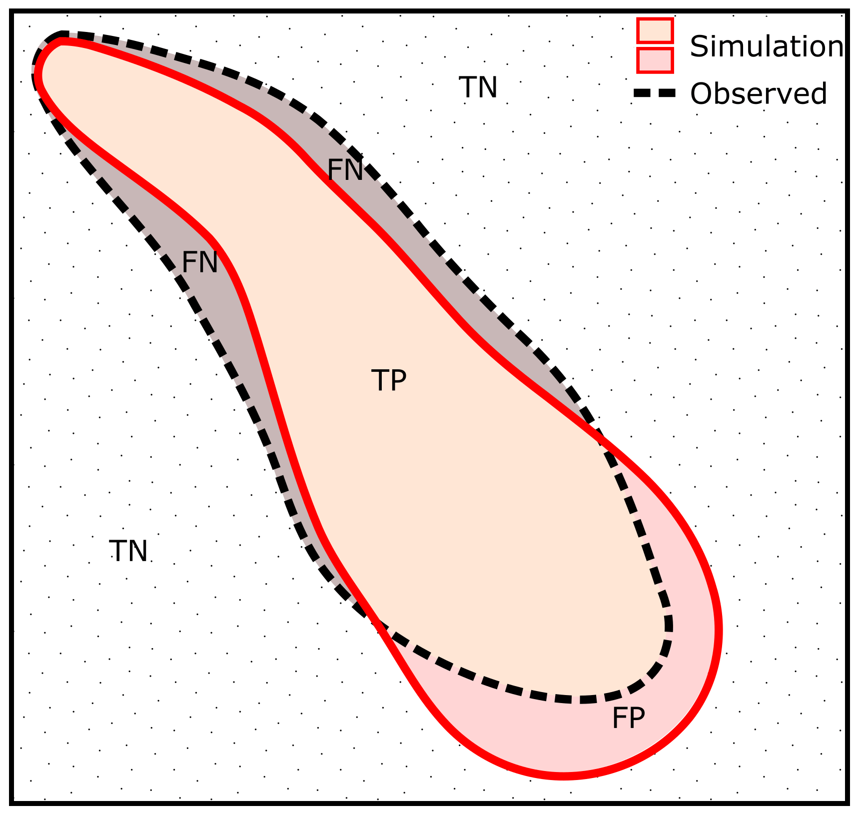
Figure 4Illustration of confusion matrix classification for simulation performance assessment. Dashed black outline represents the observed flow outline, and solid red outline represents the simulated flow outline. Areas outside of both simulated and observed flow outlines are classed as true negatives (TNs, dotted region); areas outside simulated outline but inside observed outline are classed as false negatives (FNs); areas inside both simulated and observed outline are classed as true positives (TPs); and areas inside simulated outline but outside observed outline are classed as false positives (FPs).
There is a wide range of ratios (see e.g. Sing et al., 2005) to quantify model accuracy, and there is usually no single “best” metric (Charbonnier et al., 2017). Rather, several metrics are usually analysed together to achieve a comprehensive understanding of performance. However, as demonstrated in Fig. 4, the proportion of TN values is dependent on the size of the model domain and can have significantly higher counts than other values. Therefore, for model evaluation purposes, most metrics that consider TN values in the denominator or numerator are unsuitable. Here, as with previous approaches (Charbonnier et al., 2017; Mergili et al., 2017), we calculate positive predictive value (PPV), sensitivity, and critical success index (CSI; Formetta et al., 2016; also called the Jaccard similarity coefficient) performance metrics for each flow model.
Figure 5 shows the calculated performance metrics for each flow simulation at inundation thresholds up to 10 m. The inundation threshold value is used to convert simulated flow depths into a binary (i.e. inundated/not inundated) classification, and performance curves were calculated using the ROCR package (Sing et al., 2005) in the R statistical language. The PPV, shown in Fig. 5a, is the proportion of correctly simulated (TP) areas within the simulated inundation footprint, calculated as . As FP values are in the denominator, this measure penalises over-prediction of debris flow extents. This metric increases with depth cut-off values, indicating it is less likely that simulations are incorrect in areas where deep flow is predicted. Sensitivity (Fig. 5b), the proportion of correctly simulated (TP) areas within the observed inundation footprint (), penalises under-prediction of debris flow extents and shows the opposite trend. The CSI (Fig. 5c) penalises both under- and over-prediction flow extents, calculated as the proportion of correctly simulated (TP) areas within a combined simulation and observed inundation footprint (). Values of this metric are much lower than the sensitivity or PPV as both under- and over-prediction are penalised. In effect, this metric identifies the proportion of the simulated inundation footprint that is correctly simulated. In effect, this means values of CSI less than 0.5 indicate the simulation is more “incorrect” than “correct” (more FP and FN than TP).
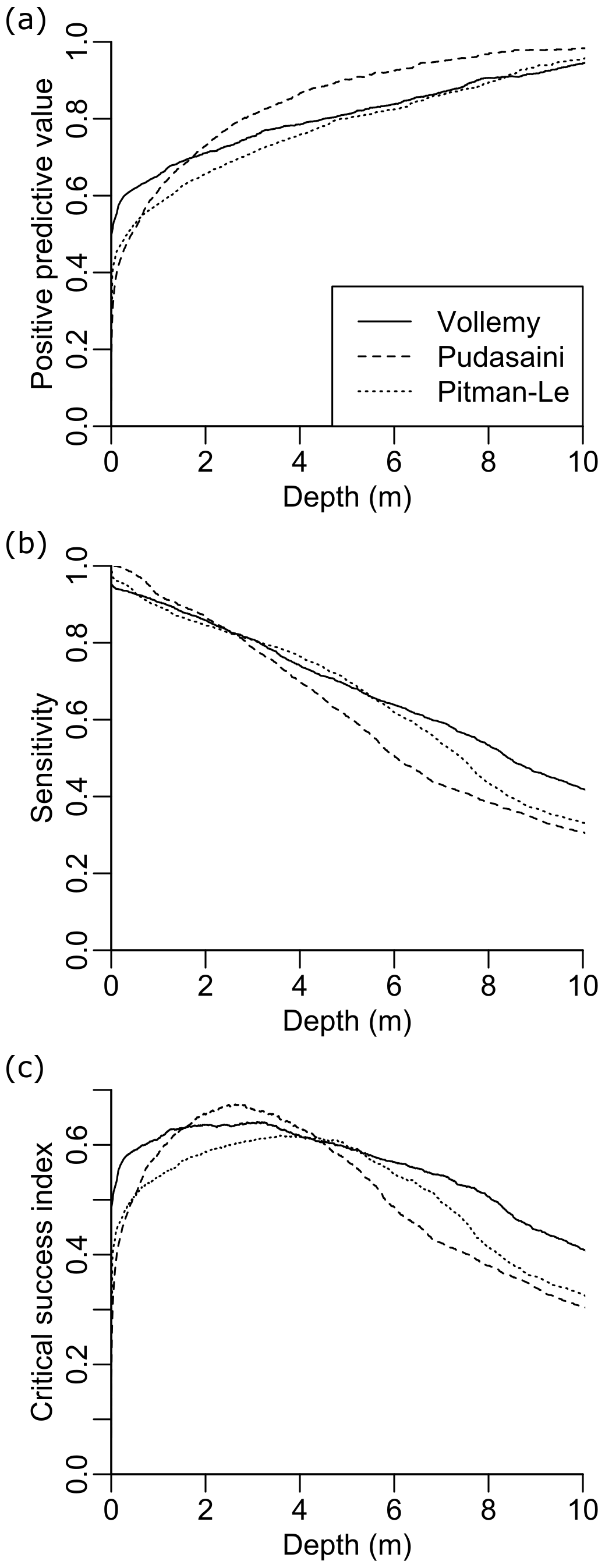
Figure 5Flow outline performance with depth for Voellmy–Salm (solid line), Pudasaini (2012) (dashed line), and Pitman and Le (2005) (dotted line) flow models. Performance metrics are (a) positive predictive value (PPV), (b) sensitivity, and (c) critical success index (CSI).
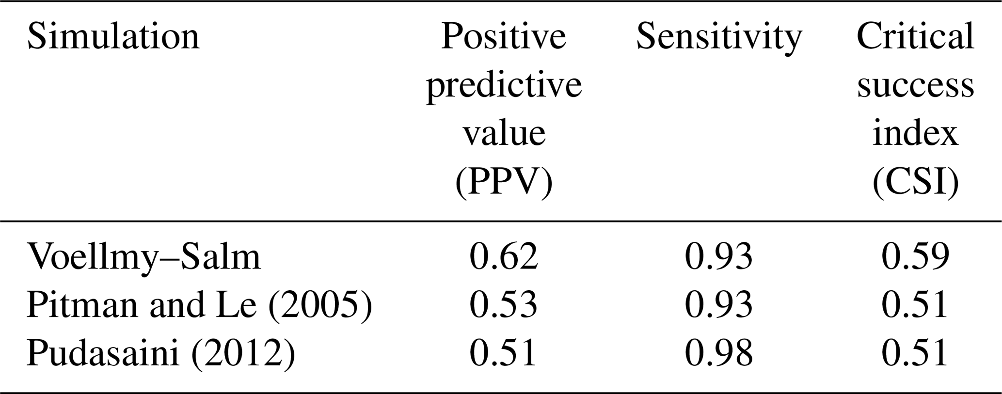
In Table 2, we report performance metrics at a depth cut-off at which CSI indicates the simulations are more “correct” than “incorrect” (0.5 m). The accuracy metrics reported here are comparable to similar flow simulation studies in which accuracy metrics are explicitly reported (e.g. Charbonnier et al., 2017; Mergili et al., 2017). However, as previously discussed, single-value metrics are useful for model comparison but can conflate and disguise sources and the distribution of error. In particular, the spatial distribution of error is not random; rather, it is related to topography (e.g. degree of confinement to the channel) and distance from source. To demonstrate this effect, the maximum flow depth for each cell (10 m resolution) was mapped to its corresponding PPV (i.e. from Fig. 5) and is shown in Fig. 6. At the centre of the debris flow, where flow depth is high, PPVs are generally higher, and the largest area of low PPVs for all simulations are most distal from the source (where flow depth is low). This indicates trends of decreasing PPV away from the source and topography affecting PPV, with areas of low topographic slope having lower PPVs. The correlation of flow depth and PPV from topographic and distance from source effects results in a degree of spatial autocorrelation in the performance metrics that is un-reported in global PPV measures.
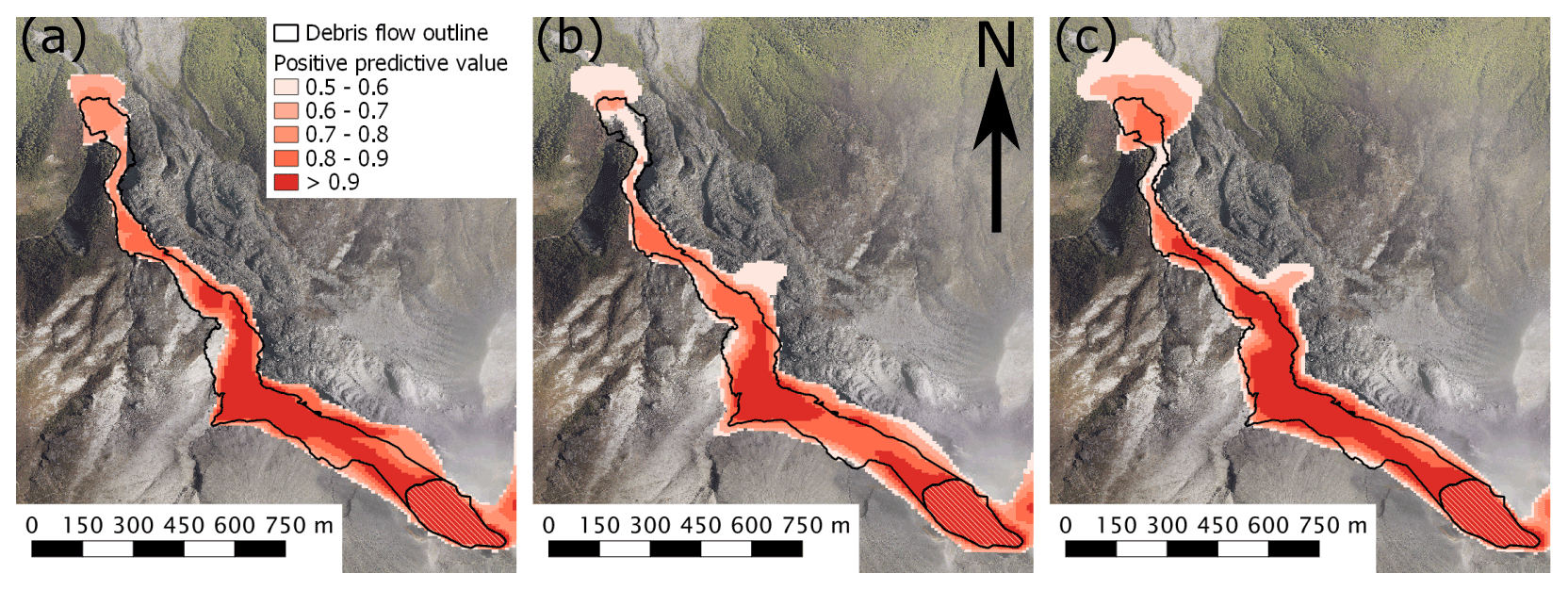
Figure 6Positive predictive values for (a) Voellmy–Salm, (b) Pitman and Le (2005), and (c) Pudasaini (2012) simulations. The observed flow and source are outlined in black. Aerial basemap sourced from LINZ Waikato Aerial Photos 2012–2013.
Table 2Pixel-pair performance assessment results for all flow simulations at a depth cut-off of 0.5 m.
4.1 Locational tolerance in performance assessment
The uncertainties in terrain data, initial conditions, model assumptions, and potential observation errors suggest that precise quantitative and locational agreement between simulated and observed debris flows are unlikely. Some level of error tolerance is therefore necessary in comparisons and would produce performance metric values more aligned with qualitative (i.e. human) assessments (Wealands et al., 2005). The spatial autocorrelation of performance metrics, shown in Fig. 6, indicate that locational tolerance may be accounted for by considering the cell neighbourhood in model comparisons.
To incorporate the influence of neighbouring cells in defining inundation footprints for model comparison, a fuzzy set approach is used. Our approach, based largely on Hagen (2003), expands classification boundaries according to a distance decay function. The classification of each cell is converted into a “fuzzy” membership vector, calculated as max(ci⋅W), where ci is the “crisp” category membership vector (e.g. for a map with inundated/not inundated categories), and W is the distance decay function. Here, we use a two-dimensional Gaussian-like weighting function:
where Wi is weighting of cell i, λ is the neighbourhood width and length (in cells), i=0 … λ−1, and the standard deviation is defined as a function of the neighbourhood size:
This technique creates a “fuzzy” quantity (between 0 and 1) that indicates the proximity of a cell to similar-valued cells.

Figure 7Fuzzy performance metrics at 3-cell (30 m), 5-cell (50 m), 7-cell (70 m), 9-cell (90 m), and 11-cell (110 m) length scales (λ) and fuzzy quantities of 0.1 (blue), 0.25 (black), and 0.5 (red) for (a) model sensitivity and (b) positive predictive value for Voellmy–Salm (solid line), Pudasaini (2012) (dashed line), and Pitman and Le (2005) (dotted line) flow models.
Figure 7 shows the performance metrics fuzzified through Eqs. (2) and (3). Regardless of fuzzy quantity, the target performance metric (sensitivity, Fig. 7a) is improved by increasing the length scale (λ) to account for spatial autocorrelation. The increase in sensitivity is associated with a commensurate decrease in the opposing performance value (PPV), shown in Fig. 7b. The greatest change in performance occurs between length scales of 10 m (i.e. model scale, no fuzzification) and 30 m (i.e. 3 model cells), and the rate of change diminishes with length scale with only marginal improvements in performance beyond 70 m (7 model cells). This indicates the approximate scale of positional error in the model, demonstrating the length scale parameter could be an alternative metric to quantify performance and evaluate models to their desired purpose. For example, a “best” model could be chosen from the model with the smallest length scale that exceeds a desired performance level or through optimising the trade-off between sensitivity and PPV beyond a given level.
The fuzzy quantity decreases the number of false negatives (and decreases false positives) in the result by expanding the zone of cells considered close to the central cell. The use of the fuzzy quantity to tune performance is not reliable at small length scales due to the discrete (cell-based) approximation of the weighting function in Eq. (2) (e.g. a fuzzy quantity less than 0.25 is not possible at 30 m length scale). As a result, the fuzzy quantity is fixed at 0.25 (the minimum value of 3-cell length scale), with length scale chosen to achieve desired performance levels.
5.1 Model suitability, calibration, and performance
In this study, we restricted our use of post-event calibration to a visual calibration within a limited bound of values similar to previous literature (Mergili et al., 2017; Sosio et al., 2012). Despite this restriction, the potential improvement in model performance appears marginal when compared to more extensive calibration procedures such as parameter sweeping (e.g. a CSI of ∼0.6 reported in Mergili et al., 2017) or rheological calibration (e.g. CSI of ∼0.5 reported in Charbonnier et al., 2017). These differences are on a similar scale to the performance differences between models in our study. Potentially, this indicates source and input (e.g. terrain) uncertainties are a greater limitation on performance than uncertainties introduced by model and parameter choice. The spatial autocorrelation in performance values (Fig. 6) also supports this assertion. Areas of deeper flow (centre of channels) are likely to be less affected by terrain uncertainties than those with shallower flows (at edges of channels). In contrast, performance of the entire simulation domain would be affected if model choice or poorly calibrated parameters were the primary source of error. This is not evident in simulations presented here, and the improvement in PPV when accounting for autocorrelation further suggests terrain error, not model error, is dominant in real-scale mass flow simulations.
5.2 Implications for hazard zonation
An advantage of the previously described fuzzy performance evaluation approach is the identification of simulation uncertainty at various length scales. This presents an avenue to generate hazard zonations and maps that incorporate areal uncertainty. For example, Fig. 8 shows debris avalanche hazard outlines generated at model scale (10 m) and a correlation function (see Eq. 2) length scale of 70 m (see caption for details on delineation of the zones). The false negative rate (i.e. 1 – model sensitivity) decreases from 0.07 to 0.01 between model and fuzzified estimates, a crucial reduction from a life safety perspective. The technique also identifies trade-offs in minimising the false negative rate, such as an increase in area and decrease in positive predictive value from 0.52 to 0.46.
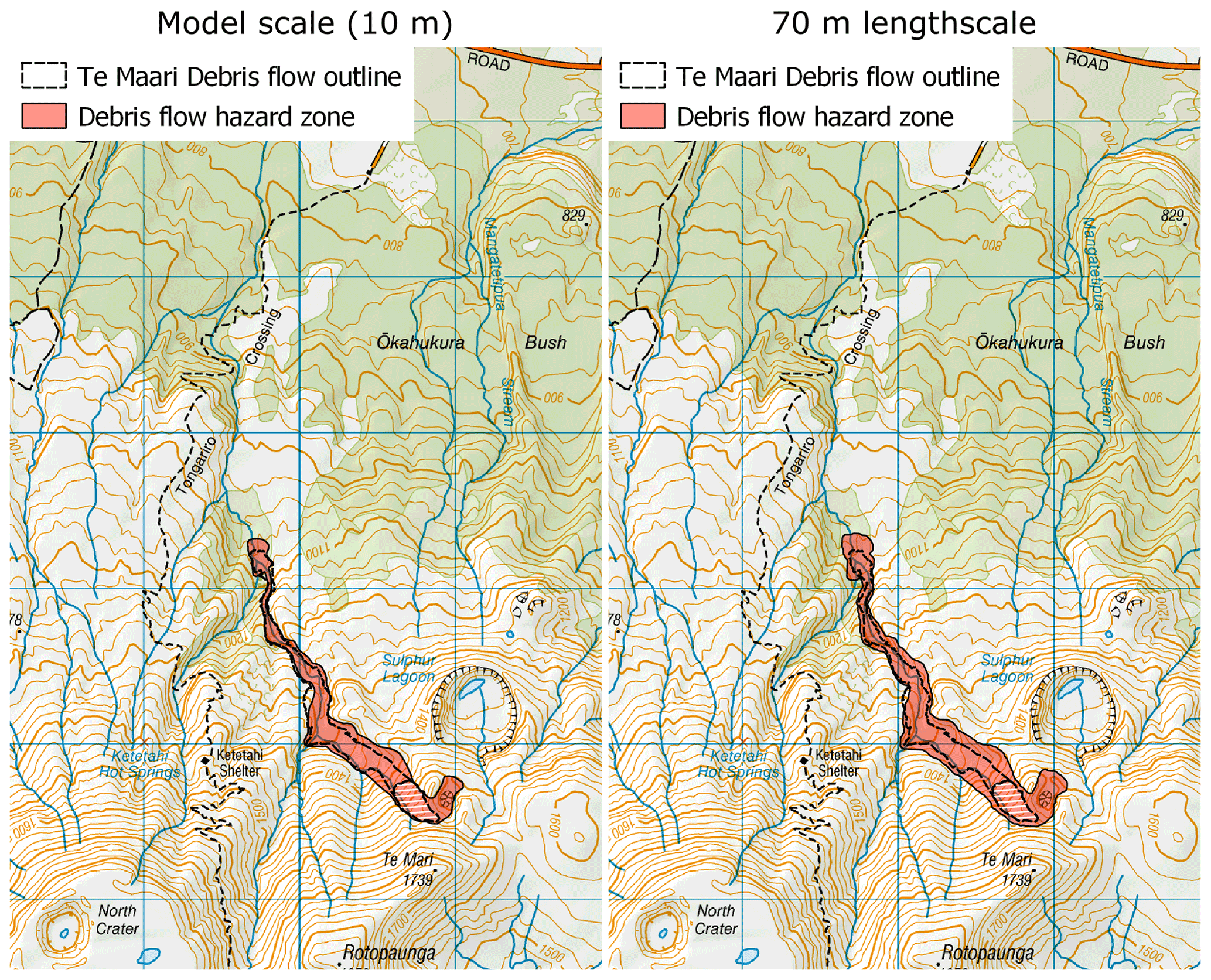
Figure 8Hazard zones generated from simulations at (left) 10 m model scale and (right) using a fuzzy length scale of 70 m. Hazard outline for model scale is generated where flow heights exceed 0.5 m. Hazard outline for 70 m scale is generated where fuzzy quantity exceeds 0.25. Hazard zones are overlain on New Zealand Topo50 map from Land Information New Zealand (LINZ). Blue grid lines are 1 km apart and are oriented north–south and east–west.
The hazard zonation approach (and fuzzification technique in general) demonstrated here can address key issues in the generation of volcanic hazard zonations by
-
quantifying and communicating model-based uncertainty, including the trade-off between hazard zone area, positive predictive value, and sensitivity, and
-
identifying appropriate scales at which to display simulated hazard data. For example, if the chosen length scale is 70 m, an appropriate hazard map scale is approximately 1:70 000 (obtained by multiplying length scale by 1000 as in Tobler, 1987).
This method can also reduce the complexity of estimating uncertainty and making decisions using simulated data to a problem that only requires judicious choice of a length scale value. However, the lack of a currently defined (mathematical) basis to parameterise length scale means that a careful consideration of hazard exposure and the acceptability of risk to exposed elements is required. This may differ between users; we therefore believe this hazard zonation process is currently best suited for use by informed stakeholders as a decision support tool rather than an automated process to generate publicly disseminated hazard zones.
The accuracy of three depth-averaged numerical models was assessed using the 2012 Te Maari debris avalanche as a benchmark. Results of the simulations show a similar qualitative accuracy of all three models to other published studies. Quantitative performance metrics of inundation area show high model sensitivity (i.e. a low proportion of false positives) with moderate values of positive predictive values and the critical success index, which are similar in scale to other published performance assessment studies.
Our investigation also demonstrates the positional dependence of model performance, specifically the positive predictive value, in which model performance (i.e. accuracy) is highest in areas of deep flow or where topography is steep with confined channels. Using this observation, a fuzzy set approach is used to incorporate locational tolerance (the covariance of location and positive predictive value) into the simulation performance assessment. We found increasing the length scale (λ) of the correlation function can increase performance metrics for a commensurate decrease in the opposing performance metric and resolution. For example, an increase in sensitivity will result in a decrease in positive predictive value.
The identification of positional uncertainty in hazard simulations has positive implications for hazard zonation and mapping. The process demonstrated here can improve desired performance metrics (e.g. sensitivity), account for uncertainty (by increasing hazard zone area), and identify trade-offs to opposing metrics (e.g. positive predictive value). This can be a valuable tool for informed stakeholders with well-quantified exposures and risk tolerances. The process is, however, less suited to publicly disseminated hazard information due to the lack of a mathematically optimum solution for length scale. An optimum solution may be identifiable, and progress in hazard zonation methodologies would benefit from deeper investigation of the trade-offs between area, length scale, and model performance to fully leverage benefits of the fuzzy performance evaluation approach.
Code to generate fuzzy membership vectors is available from the Zenodo data repository at https://doi.org/10.5281/zenodo.2797984 (Maed, 2019).
SRM developed fuzzification code, ran simulations, and prepared the manuscript with contributions from all co-authors. JP provided case study data, assisted with field studies, and reviewed and edited the manuscript. GK performed analysis on hyperspectral imagery for the case study, assisted with fieldwork, and reviewed and edited the manuscript.
The authors declare that they have no conflict of interest.
Publisher's note: Copernicus Publications remains neutral with regard to jurisdictional claims in published maps and institutional affiliations.
The authors wish to acknowledge the use of New Zealand eScience Infrastructure (NeSI) high-performance computing facilities as part of this research. New Zealand's national facilities are provided by NeSI and funded jointly by NeSI's collaborator institutions and through the Ministry of Business, Innovation & Employment's Research Infrastructure programme.
This research has been supported by the Natural Hazards Research Platform (Too big to fail? – A multidisciplinary approach to predict collapse and debris flow hazards from Mt. Ruapehu) and the Resilience to Nature's Challenges National Science Challenge “Volcanism” science programme.
This paper was edited by Giovanni Macedonio and reviewed by David Jessop, Jessica Ball, and one anonymous referee.
Aguilera, E., Pareschi, M. T., Rosi, M., and Zanchetta, G.: Risk from Lahars in the Northern Valleys of Cotopaxi Volcano (Ecuador), Nat. Hazards, 33, 161–189, https://doi.org/10.1023/B:NHAZ.0000037037.03155.23, 2004.
Bennett, N. D., Croke, B. F. W., Guariso, G., Guillaume, J. H. A., Hamilton, S. H., Jakeman, A. J., Marsili-Libelli, S., Newham, L. T. H., Norton, J. P., Perrin, C., Pierce, S. A., Robson, B., Seppelt, R., Voinov, A. A., Fath, B. D., and Andreassian, V.: Characterising performance of environmental models, Environ. Model. Softw., 40, 1–20, https://doi.org/10.1016/j.envsoft.2012.09.011, 2013.
Calder, E., Wagner, K., and Ogburn, S. E.: Volcanic hazard maps, in: Global Volcanic Hazards and Risk, edited by: Loughlin, S. C., Sparks, R. S. J., Brown, S. K., Jenkins, S. F., and Vye-Brown, C., Cambridge University Press, Cambridge, https://doi.org/10.1017/CBO9781316276273.022, 2015.
Charbonnier, S. J., Germa, A., Connor, C. B., Gertisser, R., Preece, K., Komorowski, J. C., Lavigne, F., Dixon, T., and Connor, L.: Evaluation of the impact of the 2010 pyroclastic density currents at Merapi volcano from high-resolution satellite imagery, field investigations and numerical simulations, J. Volcanol. Geoth. Res., 261, 295–315, https://doi.org/10.1016/j.jvolgeores.2012.12.021, 2013.
Charbonnier, S. J., Connor, C. B., Connor, L. J., Sheridan, M. F., Oliva Hernández, J. P., and Richardson, J. A.: Modeling the October 2005 lahars at Panabaj (Guatemala), Bull. Volcanol., 80, 4, https://doi.org/10.1007/s00445-017-1169-x, 2017.
Christen, M., Kowalski, J., and Bartelt, P.: RAMMS: Numerical simulation of dense snow avalanches in three-dimensional terrain, Cold Reg. Sci. Technol., 63, 1–14, https://doi.org/10.1016/j.coldregions.2010.04.005, 2010.
Costanza, R.: Model goodness of fit: A multiple resolution procedure, Ecol. Model., 47, 199–215, https://doi.org/10.1016/0304-3800(89)90001-X, 1989.
Coviello, V., Capra, L., Vázquez, R., and Márquez-Ramírez, V. H.: Seismic characterization of hyperconcentrated flows in a volcanic environment, Earth Surf. Proc. Land., 43, 2219–2231, https://doi.org/10.1002/esp.4387, 2018.
Darnell, A. R., Phillips, J. C., Barclay, J., Herd, R. A., Lovett, A. A., and Cole, P. D.: Developing a simplified geographical information system approach to dilute lahar modelling for rapid hazard assessment, Bull. Volcanol., 75, 713, https://doi.org/10.1007/s00445-013-0713-6, 2013.
Doyle, E. E. H., McClure, J., Johnston, D. M., and Paton, D.: Communicating likelihoods and probabilities in forecasts of volcanic eruptions, J. Volcanol. Geoth. Res., 272, 1–15, https://doi.org/10.1016/j.jvolgeores.2013.12.006, 2014.
Esposti Ongaro, T., Cerminara, M., Charbonnier, S. J., Lube, G., and Valentine, G. A.: A framework for validation and benchmarking of pyroclastic current models, Bull. Volcanol., 82, 51, https://doi.org/10.1007/s00445-020-01388-2, 2020.
Fischer, J.-T., Kowalski, J., and Pudasaini, S. P.: Topographic curvature effects in applied avalanche modeling, Cold Reg. Sci. Technol., 74–75, 21–30, https://doi.org/10.1016/j.coldregions.2012.01.005, 2012.
Foody, G. M.: Status of land cover classification accuracy assessment, Remote Sens. Environ., 80, 185–201, https://doi.org/10.1016/S0034-4257(01)00295-4, 2002.
Formetta, G., Capparelli, G., and Versace, P.: Evaluating performance of simplified physically based models for shallow landslide susceptibility, Hydrol. Earth Syst. Sci., 20, 4585–4603, https://doi.org/10.5194/hess-20-4585-2016, 2016.
Fournier, N. and Jolly, A. D.: Detecting complex eruption sequence and directionality from high-rate geodetic observations: The August 6, 2012 Te Maari eruption, Tongariro, New Zealand, J. Volcanol. Geoth. Res., 286, 387–396, https://doi.org/10.1016/j.jvolgeores.2014.05.021, 2014.
George, D. L. and Iverson, R. M.: A depth-averaged debris-flow model that includes the effects of evolving dilatancy. II. Numerical predictions and experimental tests, P. Roy. Soc. A, 470, 2170, https://doi.org/10.1098/rspa.2013.0819, 2014.
Hagen, A.: Fuzzy set approach to assessing similarity of categorical maps, Int. J. Geogr. Inform. Sci., 17, 235–249, https://doi.org/10.1080/13658810210157822, 2003.
Iverson, R. M.: The physics of debris flows, Rev. Geophys., 35, 245–296, https://doi.org/10.1029/97RG00426, 1997.
Iverson, R. M. and George, D. L.: Modelling landslide liquefaction, mobility bifurcation and the dynamics of the 2014 Oso disaster, Géotechnique, 66, 175–187, https://doi.org/10.1680/jgeot.15.LM.004, 2016.
Iverson, R. M. and Ouyang, C.: Entrainment of bed material by Earth-surface mass flows: Review and reformulation of depth-integrated theory, Rev. Geophys., 53, 27–58, https://doi.org/10.1002/2013RG000447, 2014.
Iverson, R. M., Logan, M., LaHusen, R. G., and Berti, M.: The perfect debris flow? Aggregated results from 28 large-scale experiments, J. Geophys. Res.-Earth, 115, F03005, https://doi.org/10.1029/2009JF001514, 2010.
Iverson, R. M., George, D. L., and Logan, M.: Debris flow runup on vertical barriers and adverse slopes, J. Geophys. Res.-Earth, 121, 2333–2357, https://doi.org/10.1002/2016JF003933, 2016.
Jakeman, A. J., Letcher, R. A., and Norton, J. P.: Ten iterative steps in development and evaluation of environmental models, Environ. Model. Softw., 21, 602–614, https://doi.org/10.1016/j.envsoft.2006.01.004, 2006.
Jolly, A. D., Jousset, P., Lyons, J. J., Carniel, R., Fournier, N., Fry, B., and Miller, C.: Seismo-acoustic evidence for an avalanche driven phreatic eruption through a beheaded hydrothermal system: An example from the 2012 Tongariro eruption, J. Volcanol. Geoth. Res., 286, 331–347, https://doi.org/10.1016/j.jvolgeores.2014.04.007, 2014.
Kereszturi, G., Schaefer, L. N., Schleiffarth, W. K., Procter, J., Pullanagari, R. R., Mead, S., and Kennedy, B.: Integrating airborne hyperspectral imagery and LiDAR for volcano mapping and monitoring through image classification, Int. J. Appl. Earth Obs. Geoinform., 73, 323–339, https://doi.org/10.1016/j.jag.2018.07.006, 2018.
Koch, J., Jensen, K. H., and Stisen, S.: Toward a true spatial model evaluation in distributed hydrological modeling: Kappa statistics, Fuzzy theory, and EOF-analysis benchmarked by the human perception and evaluated against a modeling case study, Water Resour. Res., 51, 1225–1246, https://doi.org/10.1002/2014WR016607, 2015.
Lube, G., Breard, E. C. P., Cronin, S. J., Procter, J. N., Brenna, M., Moebis, A., Pardo, N., Stewart, R. B., Jolly, A., and Fournier, N.: Dynamics of surges generated by hydrothermal blasts during the 6 August 2012 Te Maari eruption, Mt. Tongariro, New Zealand, J. Volcanol. Geoth. Res., 286, 348–366, https://doi.org/10.1016/j.jvolgeores.2014.05.010, 2014.
Lube, G., Breard, E. C. P., Cronin, S. J., and Jones, J.: Synthesizing large-scale pyroclastic flows: Experimental design, scaling, and first results from PELE, J. Geophys. Res.-Solid, 120, 1487–1502, https://doi.org/10.1002/2014JB011666, 2015.
McDougall, S.: Landslide Runout Analysis – Current Practice and Challenges, Can. Geotech. J., 54, 605–620, https://doi.org/10.1139/cgj-2016-0104, 2016.
Mead, S.: stuartmead/volcanoplugin: Fuzzy Location Release (FuzzyLocation) [code], Zenodo, https://doi.org/10.5281/zenodo.2797984, 2019.
Mead, S. R. and Magill, C. R.: Probabilistic hazard modelling of rain-triggered lahars, J. Appl. Volcanol., 6, 8, https://doi.org/10.1186/s13617-017-0060-y, 2017.
Mead, S. R., Magill, C., Lemiale, V., Thouret, J. C., and Prakash, M.: Examining the impact of lahars on buildings using numerical modelling, Nat. Hazards Earth Syst. Sci., 17, 703–719, https://doi.org/10.5194/nhess-17-703-2017, 2017.
Mergili, M., Fischer, J. T., Krenn, J., and Pudasaini, S. P.: r.avaflow v1, an advanced open-source computational framework for the propagation and interaction of two-phase mass flows, Geosci. Model Dev., 10, 553–569, https://doi.org/10.5194/gmd-10-553-2017, 2017.
Oberkampf, W. L. and Trucano, T. G.: Verification and validation in computational fluid dynamics, Prog. Aerosp. Sci., 38, 209–272, https://doi.org/10.1016/S0376-0421(02)00005-2, 2002.
O'Brien, J., Julien, P., and Fullerton, W.: Two-Dimensional Water Flood and Mudflow Simulation, J. Hydraul. Eng., 119, 244–261, https://doi.org/10.1061/(ASCE)0733-9429(1993)119:2(244), 1993.
Patra, A. K., Bauer, A. C., Nichita, C. C., Pitman, E. B., Sheridan, M. F., Bursik, M., Rupp, B., Webber, A., Stinton, A. J., Namikawa, L. M., and Renschler, C. S.: Parallel adaptive numerical simulation of dry avalanches over natural terrain, J. Volcanol. Geoth. Res., 139, 1–21, https://doi.org/10.1016/j.jvolgeores.2004.06.014, 2005.
Patra, A. K., Bevilacqua, A., and Safei, A. A.: Analyzing Complex Models Using Data and Statistics, in: Computational Science – ICCS 2018, Cham, 724–736, 2018.
Pistolesi, M., Cioni, R., Rosi, M., and Aguilera, E.: Lahar hazard assessment in the southern drainage system of Cotopaxi volcano, Ecuador: Results from multiscale lahar simulations, Geomorphology, 207, 51–63, https://doi.org/10.1016/j.geomorph.2013.10.026, 2014.
Pitman, E. B. and Le, L.: A two-fluid model for avalanche and debris flows, 1832, 1573–1601, https://doi.org/10.1098/rsta.2005.1596, 2005.
Pitman, E. B., Nichita, C. C., Patra, A., Bauer, A., Sheridan, M., and Bursik, M.: Computing granular avalanches and landslides, Phys. Fluids, 15, 3638–3646, https://doi.org/10.1063/1.1614253, 2003.
Procter, J., Cronin, S. J., Fuller, I. C., Lube, G., and Manville, V.: Quantifying the geomorphic impacts of a lake-breakout lahar, Mount Ruapehu, New Zealand, Geology, 38, 67–70, https://doi.org/10.1130/g30129.1, 2010a.
Procter, J., Cronin, S., Platz, T., Patra, A., Dalbey, K., Sheridan, M., and Neall, V.: Mapping block-and-ash flow hazards based on Titan 2D simulations: a case study from Mt. Taranaki, NZ, Nat. Hazards, 53, 483–501, https://doi.org/10.1007/s11069-009-9440-x, 2010b.
Procter, J. N., Cronin, S. J., Fuller, I. C., Sheridan, M., Neall, V. E., and Keys, H.: Lahar hazard assessment using Titan2D for an alluvial fan with rapidly changing geomorphology: Whangaehu River, Mt. Ruapehu, Geomorphology, 116, 162–174, https://doi.org/10.1016/j.geomorph.2009.10.016, 2010c.
Procter, J. N., Cronin, S. J., Zernack, A. V., Lube, G., Stewart, R. B., Nemeth, K., and Keys, H.: Debris flow evolution and the activation of an explosive hydrothermal system; Te Maari, Tongariro, New Zealand, J. Volcanol. Geoth. Res., 286, 303–316, https://doi.org/10.1016/j.jvolgeores.2014.07.006, 2014.
Pudasaini, S. P.: A general two-phase debris flow model, J. Geophys. Res.-Earth, 117, F03010, https://doi.org/10.1029/2011JF002186, 2012.
Rickenmann, D., Laigle, D., McArdell, B. W., and Hübl, J.: Comparison of 2D debris-flow simulation models with field events, Comput. Geosci., 10, 241–264, https://doi.org/10.1007/s10596-005-9021-3, 2006.
Salm, B.: Flow, flow transition and runout distances of flowing avalanches, Ann. Glaciol., 18, 221–226, https://doi.org/10.3189/S0260305500011551, 1993.
Savage, S. B. and Hutter, K.: The motion of a finite mass of granular material down a rough incline, J. Fluid Mech., 199, 177–215, https://doi.org/10.1017/S0022112089000340, 1989.
Scheidl, C., McArdell, B. W., and Rickenmann, D.: Debris-flow velocities and superelevation in a curved laboratory channel, Can. Geotech. J., 52, 305–317, https://doi.org/10.1139/cgj-2014-0081, 2014.
Scott, K. M., Vallance, J. W., Kerle, N., Luis Macías, J., Strauch, W., and Devoli, G.: Catastrophic precipitation-triggered lahar at Casita volcano, Nicaragua: occurrence, bulking and transformation, Earth Surf. Proc. Land., 30, 59–79, https://doi.org/10.1002/esp.1127, 2005.
Scott, W. E., Pierson, T. C., Schilling, S. P., Costa, J. E., Gardner, C. A., Vallance, J. W., and Major, J. J.: Volcano hazards in the Mount Hood region, Oregon, Open File Report 97-89, US Geol. Surv., Vancouver, WA, 14 pp., 1997.
Sheridan, M. F., Stinton, A. J., Patra, A., Pitman, E. B., Bauer, A., and Nichita, C. C.: Evaluating Titan2D mass-flow model using the 1963 Little Tahoma Peak avalanches, Mount Rainier, Washington, J. Volcanol. Geoth. Res., 139, 89–102, https://doi.org/10.1016/j.jvolgeores.2004.06.011, 2005.
Sing, T., Sander, O., Beerenwinkel, N., and Lengauer, T.: ROCR: visualizing classifier performance in R, Bioinformatics, 21, 3940–3941, https://doi.org/10.1093/bioinformatics/bti623, 2005.
Sosio, R., Crosta, G. B., and Frattini, P.: Field observations, rheological testing and numerical modelling of a debris-flow event, Earth Surf. Proc. Land., 32, 290–306, https://doi.org/10.1002/esp.1391, 2007.
Sosio, R., Crosta, G. B., and Hungr, O.: Numerical modeling of debris avalanche propagation from collapse of volcanic edifices, Landslides, 9, 315–334, https://doi.org/10.1007/s10346-011-0302-8, 2012.
Thompson, M., Lindsay, J., and Gaillard, J. C.: The influence of probabilistic volcanic hazard map properties on hazard communication, J. Appl. Volcanol., 4, 1–24, https://doi.org/10.1186/s13617-015-0023-0, 2015.
Thouret, J. C., Enjolras, G., Martelli, K., Santoni, O., Luque, J. A., Nagata, M., Arguedas, A., and Macedo, L.: Combining criteria for delineating lahar- and flash-flood-prone hazard and risk zones for the city of Arequipa, Peru, Nat. Hazards Earth Syst. Sci., 13, 339–360, https://doi.org/10.5194/nhess-13-339-2013, 2013.
Tobler, W.: Measuring spatial resolution, in: Land Resources Information Systems Conference, 12–16 May 1987, Beijing, China, 1987.
Walsh, B., Jolly, A. D., and Procter, J. N.: Seismic analysis of the 13 October 2012 Te Maari, New Zealand, lake breakout lahar: Insights into flow dynamics and the implications on mass flow monitoring, J. Volcanol. Geoth. Res., 324, 144–155, https://doi.org/10.1016/j.jvolgeores.2016.06.004, 2016.
Wealands, S. R., Grayson, R. B., and Walker, J. P.: Quantitative comparison of spatial fields for hydrological model assessment – some promising approaches, Adv. Water Resour., 28, 15–32, https://doi.org/10.1016/j.advwatres.2004.10.001, 2005.
Zeng, C., Cui, P., Su, Z., Lei, Y., and Chen, R.: Failure modes of reinforced concrete columns of buildings under debris flow impact, Landslides, 12, 561–571, https://doi.org/10.1007/s10346-014-0490-0, 2015.