La Palma landslide tsunami: calibrated wave source and assessment of impact on French territories

In this paper, we present new results on the potential La Palma collapse event, previously described and studied in Abadie et al. (2012). Three scenarios (i.e., slide volumes of 20, 40 and 80 km³) are considered, modeling the initiation of the slide to the water generation using THETIS, a 3D Navier–Stokes model. The slide is a Newtonian fluid whose viscosity is adjusted to approximate a granular behavior. After 5 min of propagation with THETIS, the generated water wave is transferred into FUNWAVE-TVD (Total Variation Diminishing version of FUNWAVE) to build a wave source suitable for propagation models. The results obtained for all the volumes after 15 min of Boussinesq model simulation are made available through a public repository.

The signal is then propagated with two different Boussinesq models: FUNWAVE-TVD and Calypso. An overall good agreement is found between the two models, which secures the validity of the results. Finally, a detailed impact study is carried out on La Guadeloupe using a refined shallow water model, SCHISM, initiated with the FUNWAVE-TVD solution in the nearshore area.

Although the slide modeling approach applied in this study seemingly leads to smaller waves compared to former works, the wave impact is still very significant for the maximum slide volume considered on surrounding islands and coasts, as well as on the most exposed remote coasts such as Guadeloupe. In Europe, the wave impact is significant (for specific areas in Spain and Portugal) to moderate (Atlantic French coast).

1 Introduction

Recent catastrophes due to exceptionally strong tsunamis (Athukorala and Resosudarmo, 2005; Mikami et al., 2012) have called for the need for extensive tsunami hazard assessment or reassessment in several countries, e.g., the National Tsunami Hazard Mitigation Program (NTHMP) for the United States (Tehranirad et al., 2015) and the Tsunamis in the Atlantic and the English ChaNnel Definition of the Effects through numerical Modeling (TANDEM) project for France (Hebert, 2014). In this context, the hazard associated with various potentially tsunamigenic sources has to be evaluated. This type of work usually covers the most frequent sources, namely coseismic displacements and submarine landslides, but long-return period sources, like volcano tsunami sources, must also be investigated. Volcanic islands may indeed have the potential to generate tsunamis (see, for instance, the recent case of Anak Krakatau; Paris et al., 2020; Grilli et al., 2019), and even megatsunamis, through a flank collapse process (Tappin et al., 2019), are known to occur relatively regularly (Elsworth and Day, 1999). Footprints of such gigantic past events are large underwater landslide debris surrounding specific oceanic islands (Masson et al., 2002) and marine conglomerates at high elevation on the flanks of other ones (Paris et al., 2018). Unfortunately, the tsunami hazard associated with volcanic islands is very difficult to determine due to the complexity of the processes involved, as well as uncertainty of the associated return period. Nevertheless, although likely very rare, these events may have such dramatic consequences that they should be taken into account in extensive hazard assessment studies. The present paper is an attempt, in the framework of the previously cited TANDEM project, to assess the potential impact on France, some parts of western Europe and remote French territories (i.e., the archipelago of Guadeloupe) of a tsunami generated by the hypothetical collapse of the Cumbre Vieja volcano (CVV) on La Palma island (Canary Islands, Spain).

This volcano (CVV) has drawn a strong interest among the scientific community since the first alarming work published on that case (Ward and Day, 2001). There have been several attempts to numerically simulate the waves generated by the Cumbre Vieja collapse. The first work (Ward and Day, 2001) was severely criticized (Mader, 2001; Pararas-Carayannis, 2002) due to the allegedly extreme landslide volume considered and the linear wave model used. In more recent computations, Gisler et al. (2006) used a 3D compressible Navier–Stokes model to simulate the slide and the resulting wave. An extrapolation of near field decay led the authors to conclude, as in Mader (2001), that this wave height would not represent such a serious threat to the east coast of North America or South America. Starting from the near field solution of Gisler et al. (2006), Løvholt et al. (2008) simulated the transoceanic propagation of the tsunami source with a Boussinesq model, therefore including dispersive effects. The propagation is shown to be very complex due to the combined effects of dispersion, refraction and interference. The authors also found smaller waves than Ward and Day (2001) but still potentially dangerous for the US coasts. Abadie et al. (2012) proposed a similar approach but one based on a 3D multiphase incompressible Navier–Stokes model to simulate the landslide and the generated wave. Because of the likelihood uncertainty, they proposed four different sliding volumes, ranging from 20 to 450 km³, obtained from a former slope stability study. The impact of these potential sources on US coasts was studied in Tehranirad et al. (2015) in the framework of the NTHMP, with propagation computed using the FUNWAVE-TVD model. In the far-field, the generated tsunamis were wave trains of three to five long-crested waves of 9 to 12 min periods. If the wave height appears very significant along the 200 m isobath (in the range of 20 m) for the largest volume considered, a strong decay is also observed due to bottom friction on the continental shelf. Moreover, besides the initial directionality of the sources, the coastal impact is mostly controlled by focusing/defocusing effects resulting from the shelf bathymetric features. Based on the same source and methodology but an inundation computed using a refined shallow water model, Grilli et al. (2016) found that the CVV causes the largest impact among possible far-field sources with a run-up of up to 20 m at the critical sites for the 450 km³ scenario.

Computations performed by Gisler et al. (2006) and Abadie et al. (2012) were both based on inviscid or quasi-inviscid slide flows. In the present paper, the computations carried out in Abadie et al. (2012) are redone, improving their accuracy by calibrating the slide fluid viscosity in order to approach a granular slide (Sects. 2.1 and 3.1) with a Newtonian model. Then, the same filtering process as in Abadie et al. (2012) is applied with the new wave sources to produce a wave signal which can be propagated by dispersive depth-averaged models (Sects. 2.2 and 3.2). The three wave sources are then propagated using FUNWAVE-TVD (Sect. 2.3.1), and the results in the Caribbean Sea, in western Europe and in France (Sect. 3.3), are analyzed. A detailed impact assessment is carried out in the Guadeloupe archipelago using refined shallow water simulations initiated with the former FUNWAVE-TVD simulations in the nearshore area.

One of the goals of the TANDEM program was also the comparison of the models developed or used by the different partners of the project for operational forecasts in order to assess potential discrepancies. Here, we take the opportunity of this La Palma case study to compare the results obtained with two Boussinesq models after long-distance propagation (Sect. 3.4), namely FUNWAVE-TVD and Calypso, which was developed by the Atomic Energy Commission (CEA), the two models employing slightly different simulation strategies. Finally, results are interpreted and discussed in Sect. 4.

2 Method

2.1 Navier–Stokes simulation of wave source

The model used for wave source computations is the Navier–Stokes multi-fluid model THETIS already described in Abadie et al. (2010) and Abadie et al. (2012) in the context of waves generated by landslides. In this 3D model, water, slide and air are simulated based on the incompressible Navier–Stokes equations for Newtonian fluids. The interfaces between phases are tracked using the volume of fluid (VOF) method. The same setup as in Abadie et al. (2012) is used in this study, so the reader is referred to this former work to find out more details on the model.

The μ(I) rheology (Jop et al., 2006) has also been implemented in THETIS to model dry, dense granular flows and has been validated by comparing it with a dry granular column collapse (Lagrée et al., 2011). The three material-dependent parameters are I₀, μ_s and Δμ. They define the friction coefficient, μ(I), which only depends on the inertial number, I. In THETIS, these variables are evaluated on each point of the slide, and the viscosity, η, is computed and imposed as the local fluid viscosity value in the Navier–Stokes equations. This gives a viscosity in the slide that is space- and time-dependent. In the present work, we used the usual values found in the literature for the model parameters, namely μ_s=0.43, Δμ=0.39 and I₀=0.27. Note that this formulation is, so far, only valid for a dry collapse (Clous and Abadie, 2019) and is therefore only used here as a reference for the initial motion.

THETIS belongs to the immiscible multiphase full Navier–Stokes type of solver. It has been validated against several benchmark cases involving tsunamis generated by 2D and 3D solid blocks (Abadie et al., 2010) and granular subaerial and submarine slides (Clous and Abadie, 2019). As such, it is more sophisticated with respect to the slide motion than models such as SAGE (Gisler et al., 2006), which rely on a compressible formulation of the equations, or the 3D Navier–Stokes model described in Horrillo et al. (2013), which employed a simplified VOF method, taking advantage of the large aspect ratio of the tsunami waves. Other recent models of interest regarding landslide tsunami generation include the NHWAVE model described in Ma et al. (2015), Kirby et al. (2016), Grilli et al. (2019) which is a two-layer sigma coordinates model for granular landslide motion and surface wave generation with a depth-averaged description of the slide and a 3D non-hydrostatic tsunami wave. For submarine landslides involving cohesive viscoplastic soils, the model BingClaw (Løvholt et al., 2017; Kim et al., 2019), based on a nonlinear Herschel–Bulkley model, incorporates buoyancy, hydrodynamic resistance and remolding, which appear crucial to properly represent the underwater landslide dynamics. The latter model has been used to study the dynamics of the Storegga Slide about 8000 years ago, as well as the 1929 Grand Banks landslide and tsunami. Finally, Eulerian–Eulerian two-phase models, such as the one described in Si et al. (2018b) and Si et al. (2018a), are very promising approaches able to describe the flow within the grains, as well as the grain–grain interactions, but their applicability to practical cases has not been demonstrated yet.

As previously mentioned, the tsunami sources proposed in Abadie et al. (2012) were computed based on Navier–Stokes simulations using a Newtonian fluid of very low viscosity (quasi-inviscid) for the slide. In 2D preliminary tests, the generated waves were shown to increase gradually when lowering the slide viscosity. So the simulations performed in Abadie et al. (2012) represent the worst case possible with this model for a given slide volume. In the present paper, the aim is to propose a more realistic source prediction by calibrating the previous Navier–Stokes model with respect to recent experimental measurements of waves generated by granular slides. The experimental results considered are Viroulet et al. (2013) (see also Viroulet et al., 2014) for subaerial slides and Grilli et al. (2017) for submarine slides.

Viroulet et al. (2013) conducted a 2D physical experiment with glass beads in order to represent an equivalent granular slide. This experiment was carried out in a flume 2.20 m long, 0.4 m high and 0.2 m wide. The beads were placed initially above water on a 45^∘ slope as in Fig. 2. Glass beads had a density of 2500 kg m⁻³ and a diameter of 1.5 mm in the first case and 10 mm in the second. Water depth was 14.8 and 15 cm for the first and second case, respectively. Four gauges monitored the surface elevation at x₁=0.45 m, x₂=0.75 m, x₃=1.05 m and x₄=1.35 m.

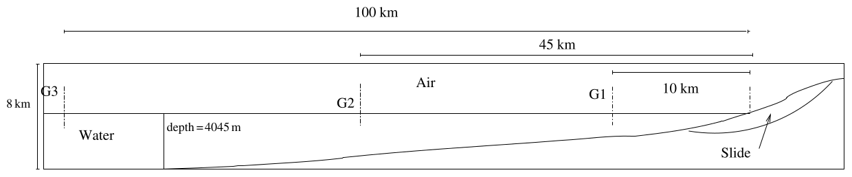
Figure 1 Cross section of the 80 km³ La Palma slide scenario considered in Abadie et al. (2012).

Figure 2 Sketch of the experiment performed in Viroulet et al. (2014).

In the numerical model used in the present paper, the slide is modeled as a fluid with a Newtonian rheology. A simulation with a μ(I) rheology was also performed for comparison purposes with the same configuration as Viroulet et al. (2013). Nevertheless, except the latter simulation, the rest of the simulations presented in this study with THETIS was carried out with a Newtonian rheology and a calibrated viscosity.

The space and time steps are Δx=5 mm, Δy=2 mm and $\mathrm{\Delta }t={\mathrm{10}}^{-\mathrm{3}}$ s. The flow is solved with the projection algorithm, and a VOF–total variation diminishing (TVD) interface tracking is performed.

For the first experimental case, presented in Viroulet et al. (2013), simulations with different values of viscosity were carried out. Figure 3 compares the height of the first wave at the four gauges. The wave simulated with the lowest viscosity, as in Abadie et al. (2012), appears to be almost twice as high as the experimental results. This first result shows the need to consider a better calibration of the model to produce more realistic results in the La Palma case. The first wave and the wave train which follows are well reproduced for a viscosity of 10 Pa s even if the slide at this viscosity is shown to be slower than in the experiment. The same overall behavior is observed in the second case with glass beads with a diameter of 10 mm, but a higher value of viscosity has to be set in order to fit the experimental wave heights. Note that the slide motion simulated is still slower than in the experiment. This may be due to the one-fluid model formulation which does not allow for the flow to pass through the granular medium as in reality. Energy transfers from slide to free surface, not detailed in the present study, were computed based on numerical results (Clous and Abadie, 2019) and show that waves are generated extremely quickly in this subaerial experiment. This is certainly why the differences observed in slide velocity after some time do not induce large wave discrepancies.

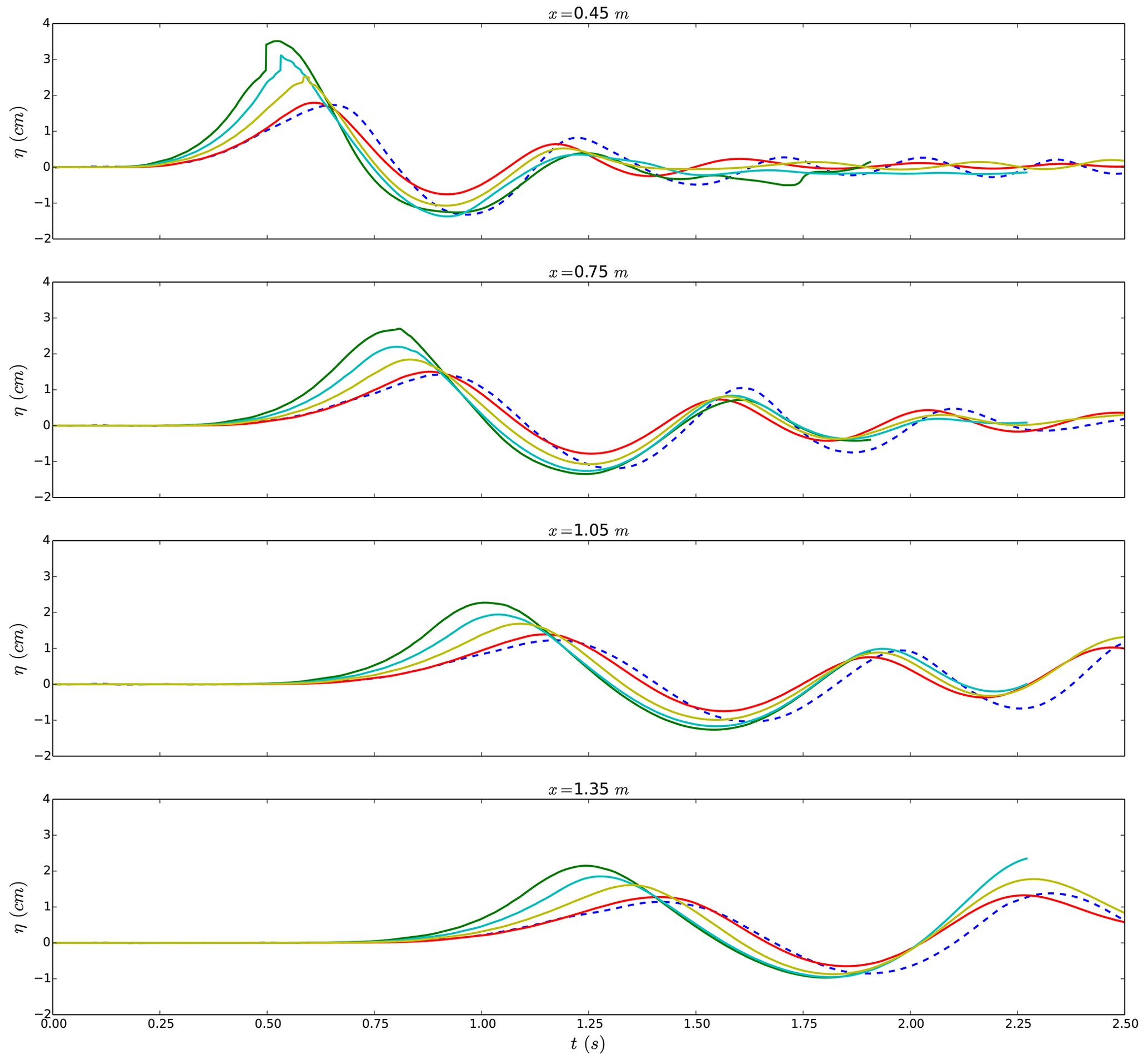
Figure 3 Free-surface elevation at the gauges for the experiment (blue dashed line) and the simulations of the first case presented in Viroulet et al. (2013) for different values of viscosity: μ=1 Pa s: green line; μ=2 Pa s: cyan line; μ=5 Pa s: yellow line; and μ=10 Pa s: red line.

The first benchmark case was also simulated with the μ(I) rheology. The results show that the wave height is quite close to the experimental results. Comparing the computation with the Newtonian fluid during the first 0.5 s when the waves are generated, the equivalent viscosity calculated with μ(I) rheology is homogeneous within the slide volume and close to the best Newtonian case. Therefore, this simulation shows that a well-calibrated Newtonian rheology can be used to model a complex granular rheology at least in this specific case for which energy transfers are very fast. This will be the approach used in the present paper.

The experiment presented in Grilli et al. (2017) was also simulated using THETIS. The experiment consisted of 2 kg of 4 mm glass beads released underwater over a slope of 35^∘ at a water depth of 0.330 m. The slide was first modeled as a Newtonian fluid with parameters defined in Grilli et al. (2017), i.e., a viscosity of 0.01 Pa s and a density of 1951 kg m⁻³. A few other viscosity values were also tested to evaluate the sensitivity of the model. The results show that with a slide viscosity of 0.01 Pa s, the first wave is higher than the experimental value, and the wave train is not correctly reproduced at the first gauge. By reducing the viscosity, the generated waves are lower. We observe that with a viscosity of 1 Pa s, the first wave is close to the experimental results, as well as the first waves in the wave train. Overall the results on wave height appear satisfactory, while the slide is still slower than in the experiment.

To extrapolate these results for the La Palma computations, the following reasoning is adopted. First, it is assumed that the real slide is well represented by the granular medium used in the experiment. This approach is not deterministic as there are important differences between this experiment and the real case, but at least it may be considered as a better assumption than the worst case scenario presented in Abadie et al. (2012).

Second, the 2D cross section of the La Palma slide in Abadie et al. (2012) is ∼8 km² compared to ∼4 km² for Viroulet's slide extrapolated at real scale. As these surfaces are of the same order, the slide dynamics are assumed to be roughly similar. Third, the La Palma slide is partially submerged but with a larger subaerial portion. Because of this, the real case would be more similar to the first experiment (Viroulet et al., 2014) than to the second one (Grilli et al., 2017).

The equivalent viscosity for the real case is then obtained by scaling the optimal viscosity obtained after calibrating the model against the experiments. Froude and Reynolds numbers should be the same at reduced and real scales, leading to

$$\begin{array}{}\text{(1)}& {\displaystyle \frac{u}{\sqrt{gh}}}={\displaystyle \frac{u^{\prime }}{\sqrt{g{h}^{\prime }}}},\text{(2)}& {\displaystyle \frac{\mathit{\rho }uh}{\mathit{\mu }}}={\displaystyle \frac{\mathit{\rho }{u}^{\prime }{h}^{\prime }}{{\mathit{\mu }}^{\prime }}},\end{array}$$

where g is the acceleration of gravity, u (u^′) a characteristic velocity, h (h^′) a characteristic length scale and μ (μ^′) the equivalent viscosity at real scale (reduced scale in parentheses). Combining the two equations leads to

$$\begin{array}{}\text{(3)}& {\displaystyle \frac{\mathit{\mu }}{{\mathit{\mu }}^{\prime }}}=\sqrt{{\displaystyle \frac{h^{\mathrm{3}}}{{h^{\prime }}^{\mathrm{3}}}}},\end{array}$$

which, for a viscosity ${\mathit{\mu }}^{\prime }=\mathrm{10}$ Pa s at reduced scale, gives $\mathit{\mu }=\mathrm{4.4}\times {\mathrm{10}}^{\mathrm{7}}$ Pa s at real scale given the length ratio. The slide considered in Abadie et al. (2012) (Fig. 1) being partially submerged, the latter viscosity value is arbitrarily reduced to $\mathit{\mu }=\mathrm{2}\times {\mathrm{10}}^{\mathrm{7}}$ Pa s to take into account the result obtained with the experiment of Grilli et al. (2017).

Based on these hypotheses, simulations were performed with three initial slide volumes corresponding to 20, 40 and 80 km³. The largest slide volume considered in Abadie et al. (2012), namely 450 km³, is not considered in this paper (see Sect. 4).

2.2 Transition from Navier–Stokes to propagation models

As noted in the original THETIS simulations presented in Abadie et al. (2012), the landslide, as modeled, continues to move for a very long time (more than half an hour), but the slide local Froude number is supercritical for only a short time (less than 100 s), and it is only during this supercritical period that the resulting tsunami wave continues to grow significantly. As a result, it is not necessary to model the entire slide runout in order to capture the generation of waves that will affect distant shorelines.

Taking the result from the THETIS model after 300 s of simulated time, which is when several wave fronts have already propagated away from the generation site, integrating velocity over depth, we transfer the state of the model to the Boussinesq wave model FUNWAVE-TVD (see Sect. 2.3.1). However, the water around the still-moving slide includes highly turbulent 3D effects that cannot be represented correctly in a Boussinesq model. To remove the residual flow (which is not expected to generate significant waves) near the slide, we apply an ad hoc filter, as determined by numerical experimentation. It consisted of multiplying the output of THETIS (i.e., free surface elevation and each velocity component) by a spatially varying function, thus removing the interior flow while keeping a smooth initial condition for FUNWAVE. This function is Gaussian with a standard deviation of 15 km, and the center is located at coordinates (−10 km, −10 km). For more details, including the validation of this approach, see Abadie et al. (2012).

After this filter is applied, local Boussinesq wave modeling is conducted on a 500 m resolution bathymetric grid taken from Global Multi-Resolution Topography (GMRT) (Ryan et al., 2009). In order to take advantage of the fully nonlinear version of FUNWAVE-TVD, a Cartesian coordinate grid system is used. To project this onto the local area, a transverse secant Mercator projection is used, which is similar to the Universal Transverse Mercator (UTM) system but centered at 28.5^∘ N and 18.5^∘ W corresponding to +68 km, +14 km. The distortion of the entire grid is less than 1 %.

After this initial phase of propagation, the results of wave elevation and horizontal velocity are transferred to larger-scale simulations to predict propagation and impact on various coastlines, as detailed in Sect. 2.3.

2.3 Models used for long-distance propagation

As dispersive effects are expected to play a significant role in this case (Løvholt et al., 2008), models based on the Boussinesq equations are required for long-distance propagation. Here, we present the results obtained with two Boussinesq models : FUNWAVE-TVD and Calypso.

2.3.1 FUNWAVE-TVD

FUNWAVE-TVD is the most recent implementation of the Boussinesq model FUNWAVE (Wei et al., 1995), initially developed and extensively validated for nearshore wave processes but equally used to perform tsunami case studies. The FUNWAVE-TVD code solves the Boussinesq equations of Chen (2006) with the adaptive vertical reference level of Kennedy et al. (2001) with either fully nonlinear equations in a Cartesian framework (Shi et al., 2012) or a weakly nonlinear spherical coordinate formulation with Coriolis effects (Kirby et al., 2013). It uses a TVD shock-capturing algorithm with a hybrid finite-volume and finite-difference scheme to accurately simulate wave breaking and inundation by turning off dispersive terms (hence solving the nonlinear shallow water, NSW, equations during breaking) once wave breaking is detected (detection based on the local wave height). The code is fully parallelized using the Message Passing Interface (MPI) protocol and efficient algorithms allowing a substantial acceleration of the computations with the number of cores. For operational uses, FUNWAVE-TVD has received many convenient features, such as the use of nested grids to refine the simulations in the interest areas or the use of heterogeneous Manning coefficients to characterize bottom friction. For the transatlantic simulations presented here, the Manning coefficient is a constant (0.025 m${}^{-\mathrm{1}/\mathrm{3}}$ s).

In the framework of the US NTHMP program, FUNWAVE-TVD has been validated for both tsunami propagation and coastal impact through an important set of analytical, laboratory and field benchmarks (Tehranirad et al., 2011). Other recent applications have allowed the validation of the model in real cases, such as the Tohoku-oki tsunami (Grilli et al., 2013).

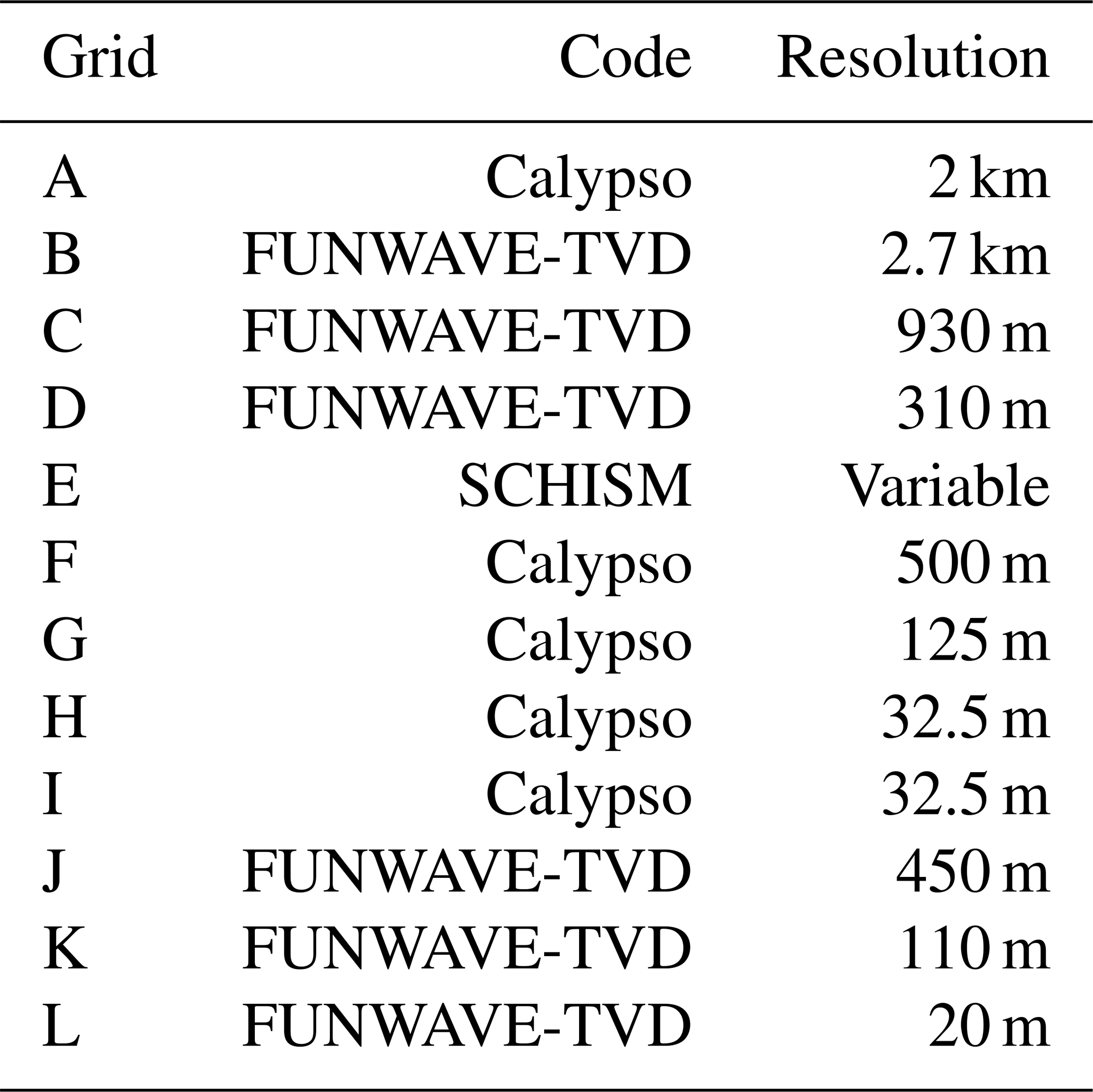
The simulation of the propagation of the tsunami to the coastlines was performed with nested grids (Figs. 4 and 5) from a 2.7 km resolution (Atlantic Ocean) to resolutions of 930 m (Antilles), 450 m (north Atlantic area), 310 m (Guadeloupe archipelago), 110 m (Aquitaine region) and 20 m (Gironde estuary).

Figure 4 Computational domains for Calypso at 2 km (A) resolution in black, FUNWAVE-TVD at 2.7 km (B), 930 m (C) and 310 m (D) resolutions in red, and SCHISM at variable resolution (E) in green. Bathymetric contours range from −500 to −7500 m every 1000 m. Gauges 1, 2 and 3 are marked by white and blue points.

Figure 5 Computational domains for Calypso at 500 m (F), 125 m (G) and 32.5 m (H and I) resolutions in black and FUNWAVE-TVD at 450 m (J), 110 m (K) and 20 m (L) resolutions in red. After the −50 m contour, bathymetric contours range from −100 to −500 m every 100 m and then from −1000 to −4000 m every 1000 m. Gauges 4, 5, 6 and 7 are marked by the white and blue points.

2.3.2 Calypso

Calypso is a code developed by CEA and used for tsunami propagation (Poupardin et al., 2017; Gailler et al., 2015). The user can choose to solve either the nondispersive (nonlinear shallow water, NSW) or dispersive (Boussinesq model following Pedersen and Løvholt, 2008) nonlinear longwave equations, written in spherical coordinates. A Crank–Nicolson scheme for the temporal discretization and a finite-difference scheme for spatial derivatives are used to solve both NSW and Boussinesq equations. For the Crank–Nicolson scheme, an iterative procedure enables the solving of the implicit set of equations. The convergence criteria are applied to the continuity equation. The spatial discretization uses centered differences for linear terms, as well as for advection terms. For Boussinesq equations, the implicit momentum equations are solved by alternating implicit sweeps in the x and y components using an alternating direction implicit (ADI) method. For a given direction, the dispersion terms in the other direction are discretized explicitly. For each direction (x and y), a tridiagonal system of equations is then solved at each iteration, following Pedersen and Løvholt (2008). The numerical scheme of Calypso has been described in Poupardin et al. (2018).

Four levels of nested grids are used in this computation (Figs. 4 and 5). The mother grid covers the Canary Islands and a large part of the Atlantic Ocean to the French coasts. It is a 2 km resolution grid with a total of 1351 cells × 1298 cells. The second grid of 1294 cells × 1404 cells covers all the French Atlantic Ocean coastline and the north of Spain at a 500 m resolution. Four grids are used to simulate the propagation of water waves in coastal regions: the so-called “Brittany” grid covers a large region in the south of Brittany at a 125 m resolution, the “Gironde” grid covers the mouth of the Gironde estuary at a 125 m resolution, and the “Saint-Jean-de-Luz” grids with the first grid at 125 m resolution and a smaller one at 32.5 m resolution which covers the bay of Saint-Jean-de-Luz in the southwest of France.

In the simulation performed, the offshore propagation was simulated by using the Boussinesq model to take into account the dispersive effects in the Atlantic Ocean, and then NSW equations are solved in the daughter grids in order to reduce the computation time.

2.3.3 Locations of numerical output

The first synthetic gauge (Gauge 1), located west in the vicinity of the Canary archipelago, is used to analyze the wave at the beginning of the event.

In the Caribbean Sea, the tsunami wave features close to the Guadeloupe archipelago will be detailed. The latter is located 16^∘ N and 61^∘ W in the Lesser Antilles at 4600 km from the Cumbre Vieja volcano. It is made up of four main groups of islands (Fig. 6) with a total surface of 1628 km². Two synthetic gauges are used in this area: gauges 8 and 9, respectively, north and south of Guadeloupe island.

In Europe, the following synthetic gauges are used (Figs. 4 and 5): Gauge 2 south of Portugal and Spain to evaluate the impact in this region, Gauge 3 in the French abyssal plain, Gauge 4 on the continental shelf off the French Atlantic coast, and gauges 5, 6 and 7 located on the French coastline (in front of the Gulf of Morbihan, near the Gironde estuary and at the entrance of the Saint-Jean-de-Luz bay). The locations, coordinates and depths of the nine gauges are provided in Figs. 4, 5 and 6 and in Table 1.

Figure 6 Guadeloupe archipelago and locations of gauges 8 and 9 and of the cities of Bouillante, Le Gosier, Le Moule and Desirade.

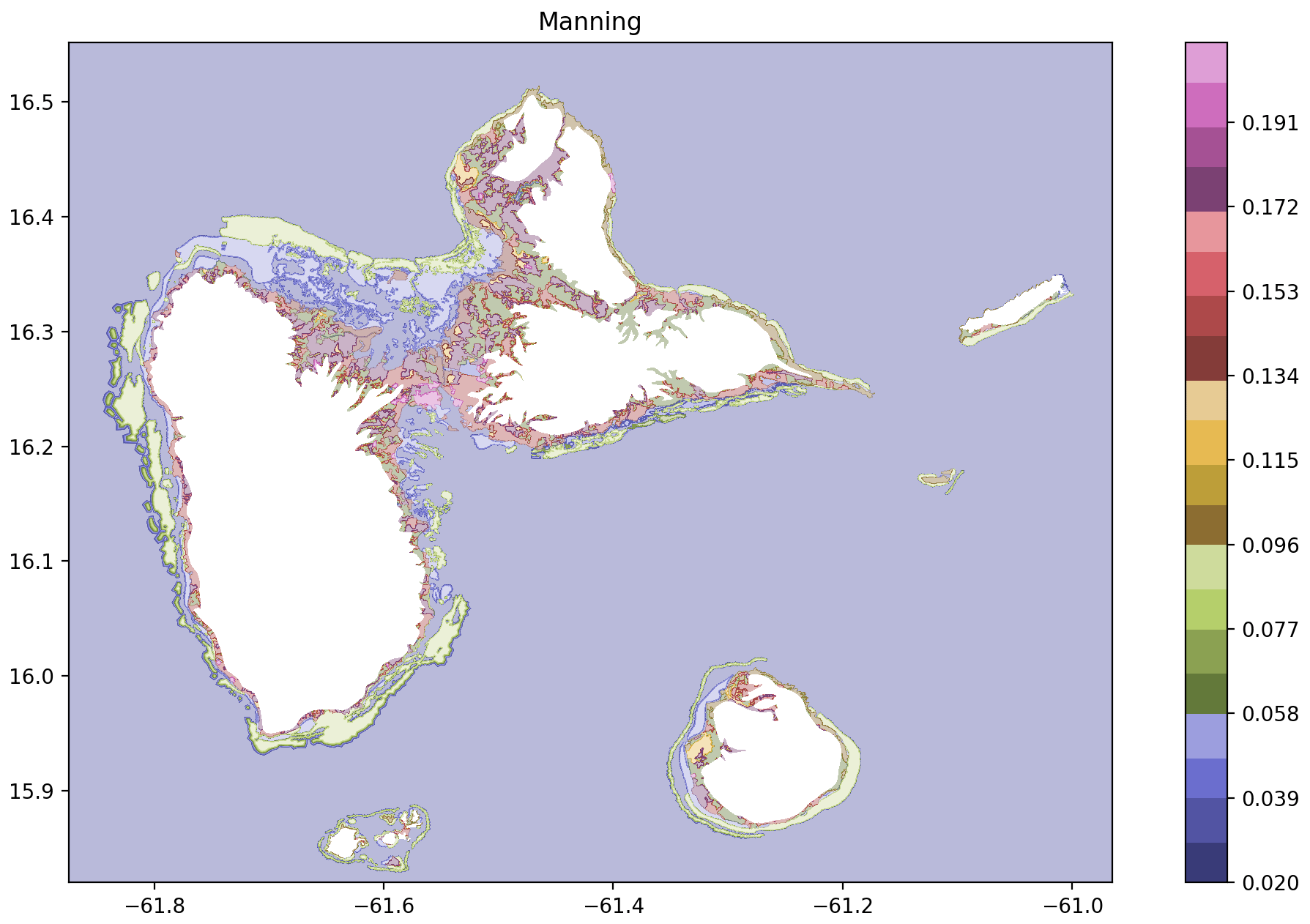
Figure 7 Values of Manning coefficient as a function of land use in Guadeloupe.

Table 1 Summary of locations of numerical output (see Fig. 4 for gauges 1, 2 and 3, Fig. 5 for gauges 4, 5, 6 and 7, and Fig. 6 for gauges 8 and 9).

Table 2 Summary of grid characteristics (see Fig. 4 for footprints of grids A, B, C, D and E and Fig. 5 for footprints of grids F, G, H, I, J, K and L).

2.4 Tsunami impact assessment

Independent of the wave signal quality, an accurate assessment of the impact of a given tsunami also requires refined computations on nested refined grids including local friction coefficients and an accurate knowledge of the bathymetry and the topography. In the present study, this extensive work was performed in La Guadeloupe. For this archipelago, the transoceanic propagation is performed using the code FUNWAVE-TVD, while nearshore propagation and inundation are carried out with SCHISM.

Semi-implicit Cross-scale Hydroscience Integrated System Model (SCHISM) (Zhang et al., 2016) is a derivative product of the SELFE model (Zhang and Baptista, 2008a). Although the code is able to solve the 3D Reynolds-averaged Navier–Stokes equations in hydrostatic or non-hydrostatic mode, in this study only one sigma layer is used, and equations are depth-integrated leading to 2D NSW equations with additional source terms for Coriolis effect, bottom friction dissipation and horizontal eddy viscosity in the momentum equation.

A hot start is made from the wave train of the FUNWAVE-TVD grid over the SCHISM unstructured grid at t=18900 s (i.e., 5 h 30 min after the volcano collapse). At this time, the first wave is about 180 km east from La Désirade. For these specific simulations along the Guadeloupe coastline and for the aerial part where specific features may obstruct the water flow inland, resolution reaches 10 m. The inundation process relies on a specific inundation algorithm that is detailed and benchmarked in Zhang and Baptista (2008b). The Manning coefficient is adjusted as a function of the land use, as shown in Fig. 7. For the submerged area, 10 classes of Manning values were used, while 50 classes have been used for the aerial domain based on the CORINE Land Cover dataset (Büttner et al., 2004). In order to avoid reflection along the domain limit, boundary conditions are set to Flather type (Flather, 1976). This extensive work could not be carried out for the entire French metropolitan coastlines, and, in this case, maximum flow depth is therefore used as a proxy to estimate wave impact.

3 Results

3.1 Wave source computation

Figures 8 and 9 provide the complete sequence of the computed slide contours, thicknesses and related water surface elevations for the 80 km³ scenario, as obtained in Abadie et al. (2012) and in the present computation considering a viscous flow with a viscosity of 2×10⁷ Pa s. With a higher viscosity, the slide dynamics and the resulting wave generation changes significantly compared to the inviscid case for the 80 km³ volume case. The slide is much slower, more compact and regular in shape during the energy transfer to water surface.

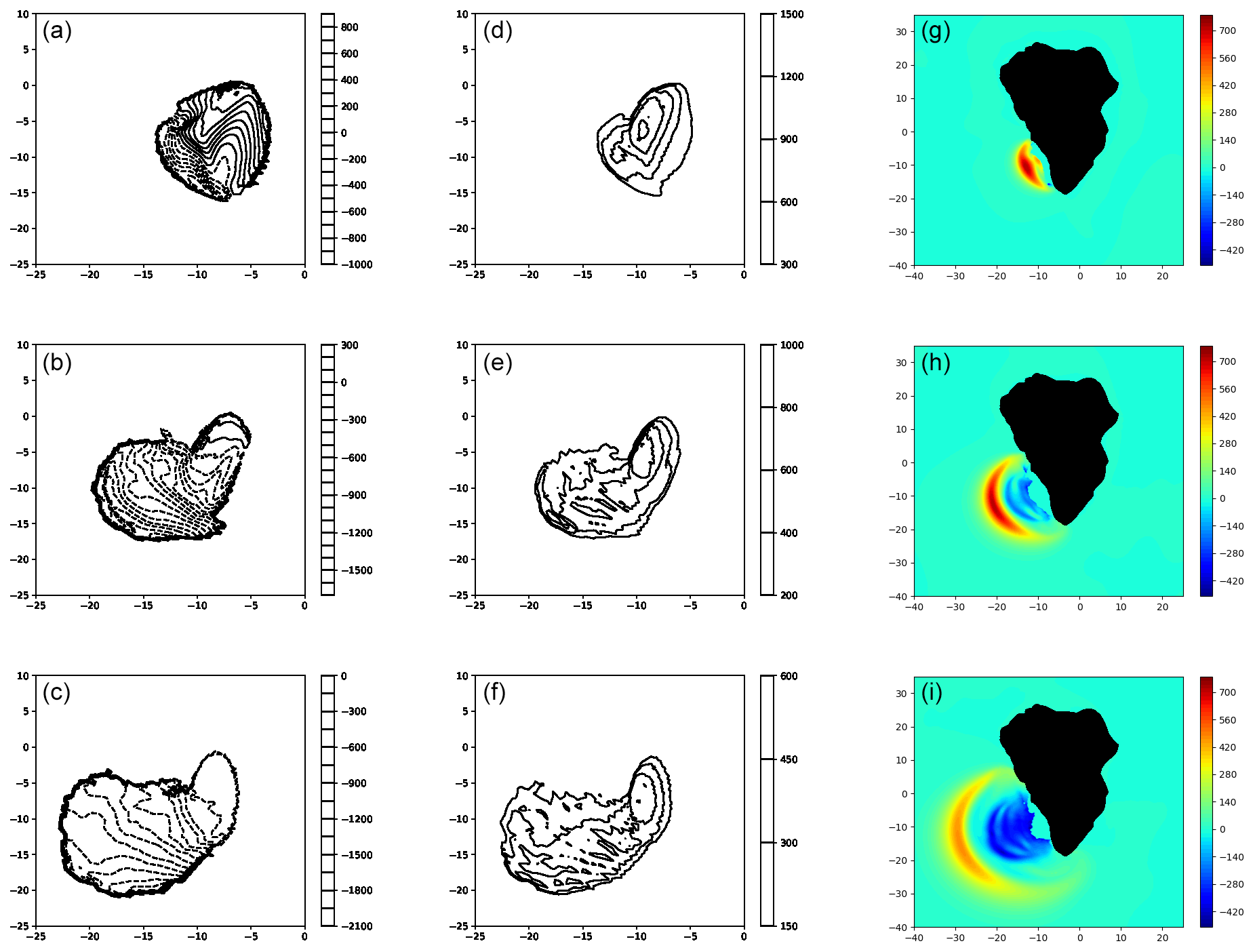
Figure 8 Snapshots of slide upper free surface, thickness and corresponding water-free surface for the inviscid case (Abadie et al., 2012) (a–c, d–f, g–i), respectively, for the 80 km³ scenario at t=60 s (a, d, g), 120 s (b, e, h) and 180 s (c, f, i).

Figure 9 Snapshots of slide upper free surface, thickness and corresponding water-free surface for the present study (i.e., viscous slide with a viscosity of 2 × 10⁷ Pa s; a–c, d–f and g–i) for the 80 km³ scenario at t=60 s (a, d, g), 120 s (b, e, h) and 180 s (c, f, i).

The bulge, which was very developed in the previous case (Fig. 10), is scarcely noticeable, although it still exists (Fig. 11). The slide tip is also slower (∼30 m s⁻¹; Fig. 11b) compared to the original simulation (∼100 m s⁻¹; Fig. 10). The rear part of the slide, where the velocity is maximum, is still very fast (∼120 m s⁻¹) at the initial stage of the process (Fig. 11a), but then the maximum velocity decreases to about 50 m s⁻¹ (Figs. 11b and c).

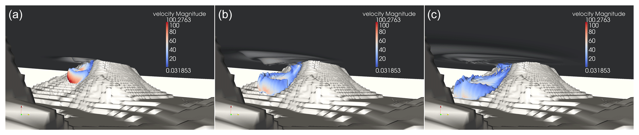
Figure 10 THETIS 3D computations for 80 km³ slide volume. Snapshots of a 0.1 slide volume fraction contour colored by velocity magnitude at t=100 s (a), 200 s (b) and 300 s (c). Inviscid slide from Abadie et al. (2012).

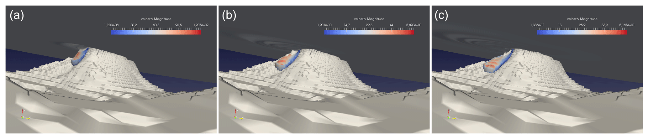
Figure 11 THETIS 3D computations for 80 km³ slide volume. Snapshots of a 0.1 slide volume fraction contour colored by velocity magnitude at t=102 s (a), 230 s (b) and 342 s (c). Slide viscosity is 2×10⁷ Pa s.

As a consequence of lower velocity and slide cross-section reduction, the wave train generated is significantly less energetic than in the inviscid case (Figs. 8 and 9). Nevertheless, the sequence of wave formation shows similarities with the generation of the first free surface positive elevation reaching 400 m in the new case (compared to 800 m previously) at t=90 s, which then exhibits a radial decrease and frequency dispersion. Additionally, the very large depression of the mean sea water level, observed at the end of the wave generation process in the previous inviscid case, is less visible in the new simulation.

For this volume, after almost 10 min of propagation, the leading wave, which was previously about 80 m high, only reaches ∼30 m in the new viscous slide case (Fig. 12c). Note that the wave energy focus has the same direction in both cases (i.e., 20^∘ south of west).

Figure 12 THETIS 3D computations for the 80 km³ slide scenario at t≈ 560 s: (a) inviscid slide, (b) slide viscosity 2×10⁷ Pa s, and (c) free surface elevations along the cross section A–B (a). Inviscid slide: continuous line; viscous slide: dotted line.

Figure 9 is not repeated for smaller slide volumes (i.e., 20 and 40 km³) as the slide evolution and wave train formation sequence show a very similar pattern as compared to the 80 km³ case.

Nevertheless, there is a significant variation in wave amplitude depending on the slide volume considered (Fig. 13). At t=5 min, the leading wave is ∼80 m high in the largest slide volume scenario (i.e., 80 km³) and is only 50 and 20 m for smaller slide volumes (40 and 20 km³, respectively).

3.2 Filtered solution

Taking the THETIS solution (Fig. 13) after the initial 5 min of propagation and applying the filter described in Sect. 2.2, the subsequent wave propagation is simulated with the Boussinesq wave model FUNWAVE-TVD with a 500 m grid for an additional 15 min, which is sufficient to consider the interaction between the tsunami and the nearby islands.

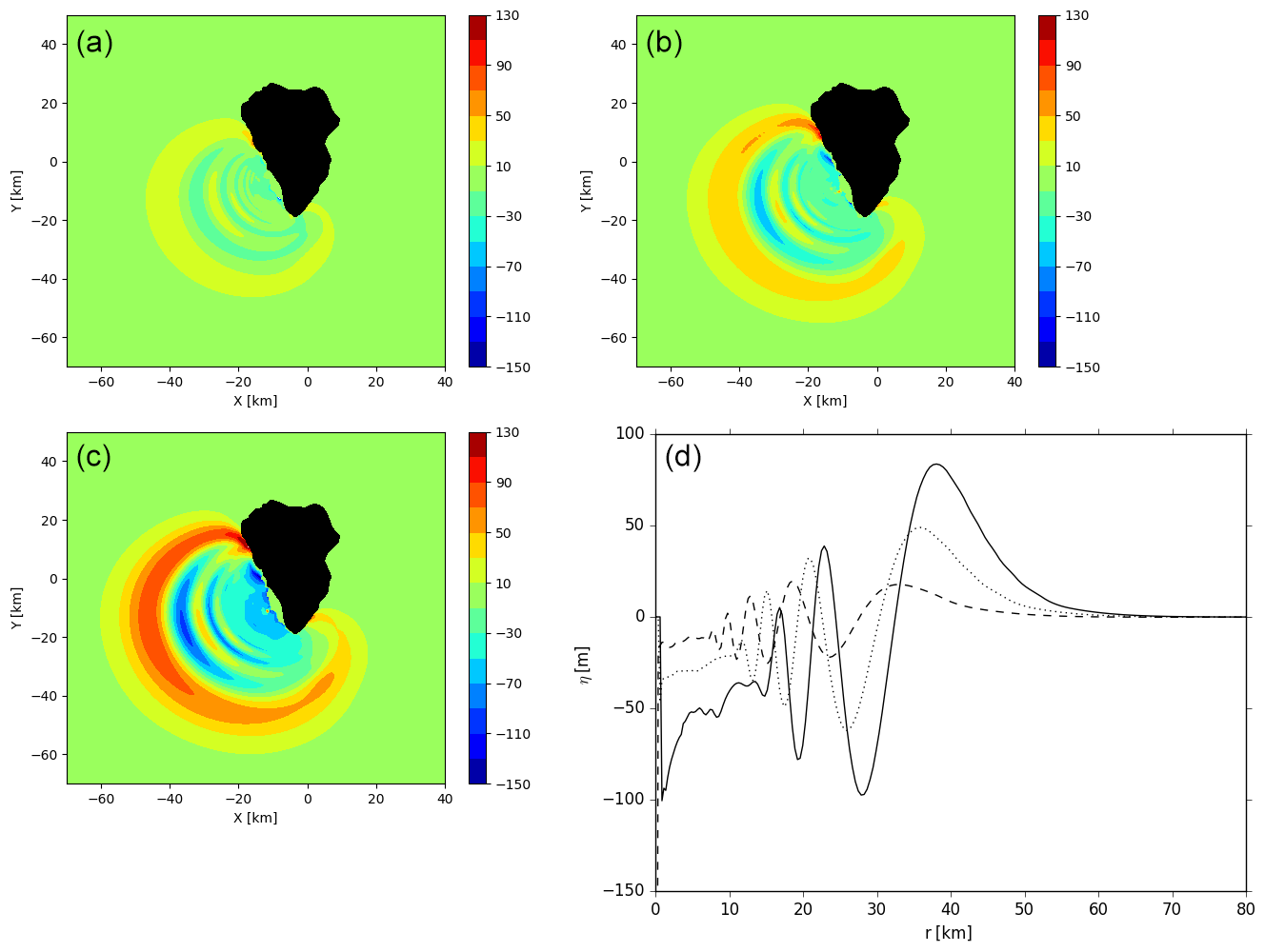
Figure 13 THETIS 3D computations for 20 km³ (a), 40 km³ (b) and 80 km³ (c) slide scenarios at t=5 min. (d) Free surface elevations along section A–B of the left frame of Fig. 12. Slide viscosity is 2 × 10⁷ Pa s. Slide volume of 80 km³: continuous line; slide volume of 40 km³: dotted line; slide volume of 20 km³: dashed line.

The effect of the filtering can be seen clearly in Fig. 14, in which flow near La Palma is strongly damped but the leading waves are unaffected. As shown by Abadie et al. (2012), this has been found to better represent the first several wave fronts and the overall wave field, as compared to an unfiltered solution.

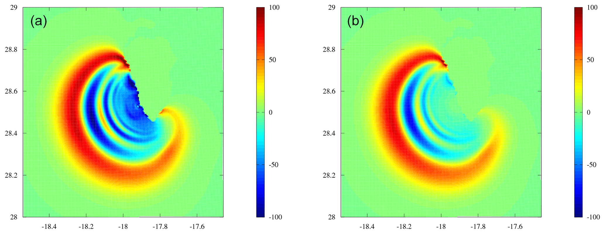
Figure 14 Region around Cumbre Vieja volcano after 5 min of simulated time with THETIS for the 80 km³ slide scenario: (a) wave elevation for the initial solution from THETIS and (b) filtered state which is used to initialize FUNWAVE-TVD.

The potential dispersive character of the wave train can be assessed by investigating the frequencies present in the wave spectrum. To that purpose, the wave signal close to the source in the direction of the maximum wave energy and the associated Fourier transform is presented in Fig. 15. At this location, the depth is 4432 m. Linear waves can be considered as shallow water waves if their respective wave length L verifies L>20 h. Still considering linear wave theory, this condition is only met for wave periods less than 4 min at this particular depth. Hence, the wave energy included in the frequency band 1 to 4 min, which is obviously not negligible in Fig. 15, can be considered as a superposition of intermediate water waves whose celerity depends of the period, not only on depth. For this part of the spectrum, which represents approximately 25 % of the overall wave train energy, dispersion is expected to occur during the next propagation phase. Note that the frequency band concerned with dispersion will evolve during the propagation with a depth increase or decrease.

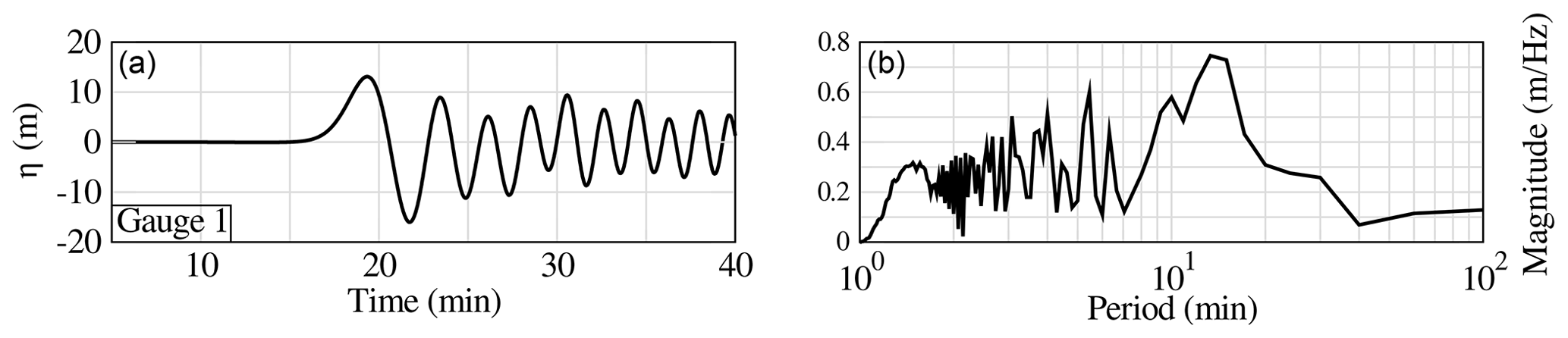
Figure 15 Surface elevation (m; a) and associated Fourier transform (b) for the 80 km³ scenario at Gauge 1 close to the source. The time takes into account the first 20 min of the slide and tsunami generation.

The resulting wave elevation and velocity fields (e.g., Fig. 16) are used as initial conditions in FUNWAVE-TVD and Calypso.

Figure 16 Region around the Canary Islands 20 min after the beginning of the event (after 5 min of simulated time with THETIS and 15 min of simulated time with FUNWAVE-TVD) during the 80 km³ slide volume scenario: (a) wave elevation and (b) horizontal water velocity magnitude.

3.3 Propagation: FUNWAVE-TVD Results

Figure 17 shows the free surface signal at several selected points (Figs. 4, 5 and 6) for the 80 km³ scenario. The surface elevation reaches 0.75 m at Gauge 2 between the south of Portugal and the north of Morocco (followed by a trough of the same amplitude) and around 0.15 m at Gauge 3 in the abyssal plain of the Bay of Biscay. These results are approximately consistent with a r⁻¹ propagation attenuation. Gauge 4 is located right after the beginning of the continental shelf. The increase in wave height is not very significant compared to Gauge 3 due to the large wavelength. Closer to the coast, the wave shoaling appears more significant with waves reaching about 0.40 m in southern Brittany, 0.25 m in the Gironde estuary and 0.40 m in Saint-Jean-de-Luz. Taking the first free surface increase as an indicator, respective tsunami arrival times are 1 h 30 min, 2 h 50 min, 3 h 30 min, 4 h 15 min, 4 h 4 min and 3 h 50 min of propagation, respectively, at gauges 2 to 7.

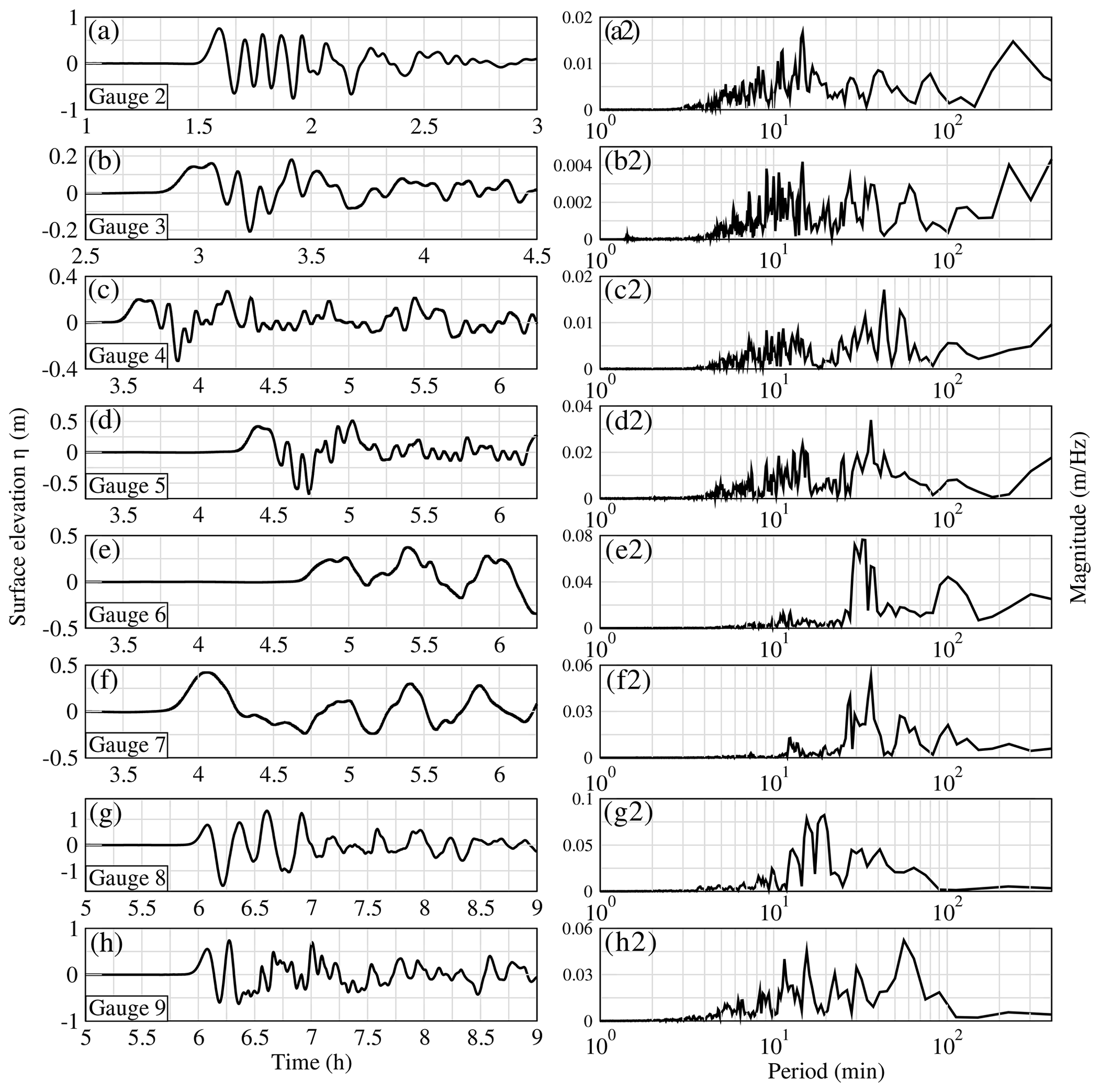
Figure 17 Surface elevations (m) (left column) and Fourier transforms (right column) for the 80 km³ scenario at Gauge 2 in southern Portugal (a and a2), Gauge 3 in the abyssal plain of the Bay of Biscay (b and b2), Gauge 4 on the continental shelf of the Bay of Biscay (c and c2), Gauge 5 in southern Brittany (d and d2), Gauge 6 in the Gironde estuary (e and e2), Gauge 7 in Saint-Jean-de-Luz (f and f2), and gauges 8 and 9, respectively, north (g and g2) and south (h and h2) of Guadeloupe, computed by FUNWAVE-TVD. The time takes into account the first 20 min of the slide and tsunami generation.

Near Guadeloupe (Fig. 17g and h), the waves reaching the coasts are still significant with the first elevation of 0.75 m at Gauge 8 and 0.5 m at Gauge 9. Note that the second wave, which also features a large trough, appears to be the largest in this area.

The frequency content of the wave signal for the 80 km³ scenario at the different gauges is also shown in Fig. 17. As expected, due to dispersion, waves involving periods smaller than 4 min, whose respective celerity is smaller, are no longer visible in the spectrum whichever gauge is considered. In front of the French Atlantic coast and in southern Brittany (i.e., Gauge 4 and Gauge 5, respectively), the signal is made up of two main frequency bands respectively centered on 10 and 40 min. The propagation toward the southern parts of the Bay of Biscay also shows a gradual decrease in the energy fraction associated with the highest frequencies (i.e., T<30 min). Hence, in Saint-Jean-de-Luz and in the Gironde estuary, the signal is dominated by wave periods between 30 and 40 min with also some energy remaining in the lower frequencies (mainly 100 min). This is probably due to the fact that only the largest wavelengths are able to refract enough to reach these locations. We also note that the very low-frequency wave signal component (T>200 min) present in gauges 2 and 3 is decreased in gauges 4, 5 and 6 and not present in Gauge 7. For Guadeloupe (gauges 8 and 9), compared to the wave signal close to the source (i.e., Gauge 1), high frequencies involving periods less than 10 min are no longer observable, and the signal is mainly composed of waves between 10 and 100 min period. This is probably a manifestation of dispersion as during the transoceanic propagation, the wave train meets several time depths larger than 6000 m.

The wave train generated by the 20 km³ slide (Fig. 18) shows very similar frequency spatiotemporal evolution with less energy and no low-frequency motion (i.e., T>100 min). (Note that we observe a lag time of 5 to 10 min for the arrival times between the two slide scenarios.) The case of 40 km³ is not presented as its characteristics can be deduced from the two former ones.

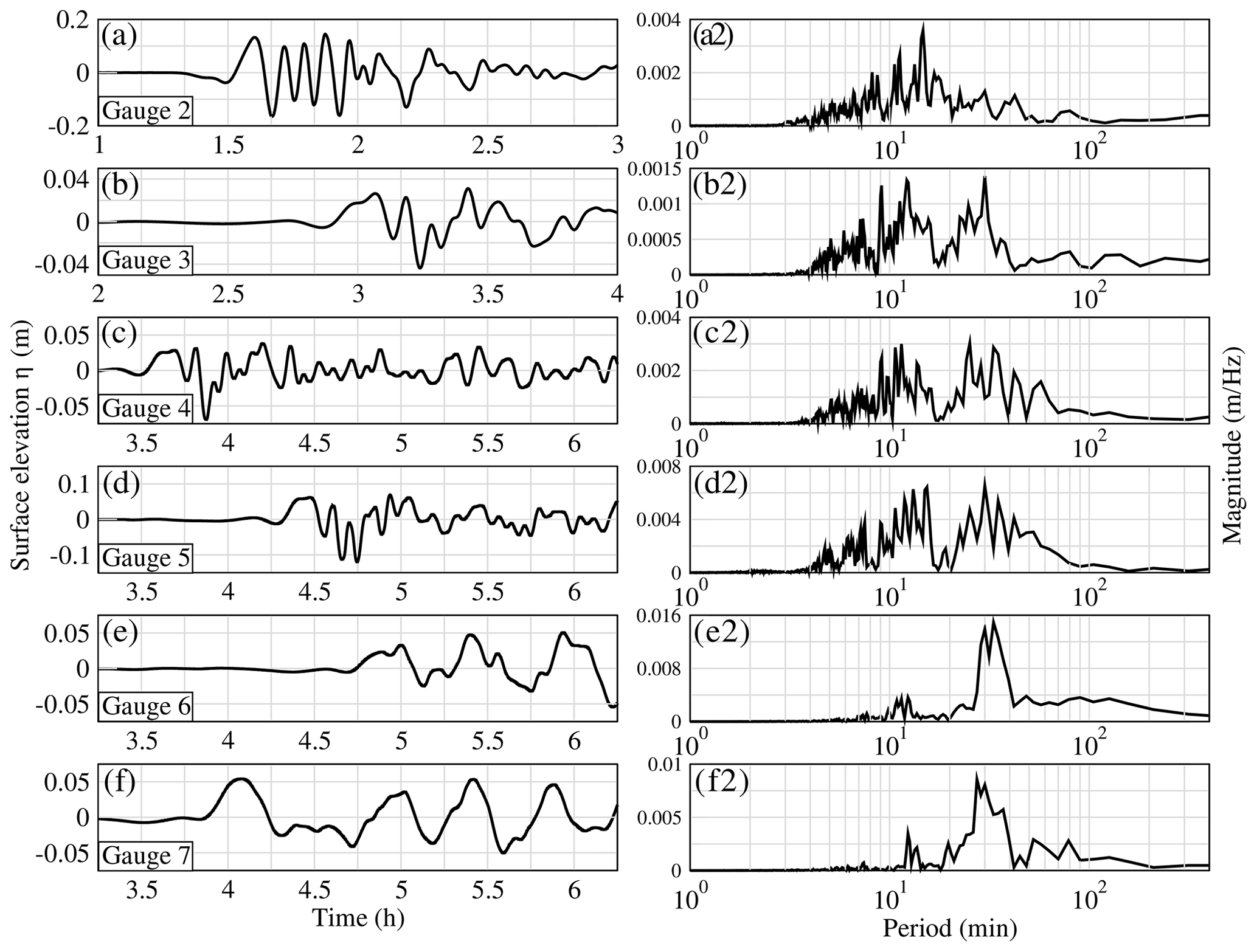
Figure 18 Surface elevations (m) (left column) and Fourier transforms (right column) for the 20 km³ scenario at Gauge 2 in southern Portugal (a and a2), Gauge 3 in the abyssal plain of the Bay of Biscay (b and b2), Gauge 4 on the continental shelf of the Bay of Biscay (c and c2), Gauge 5 in southern Brittany (d and d2), Gauge 6 in the Gironde estuary (e and e2) and Gauge 7 in Saint-Jean-de-Luz (f and f2) computed by FUNWAVE-TVD. The time takes into account the first 20 min of the slide and tsunami generation.

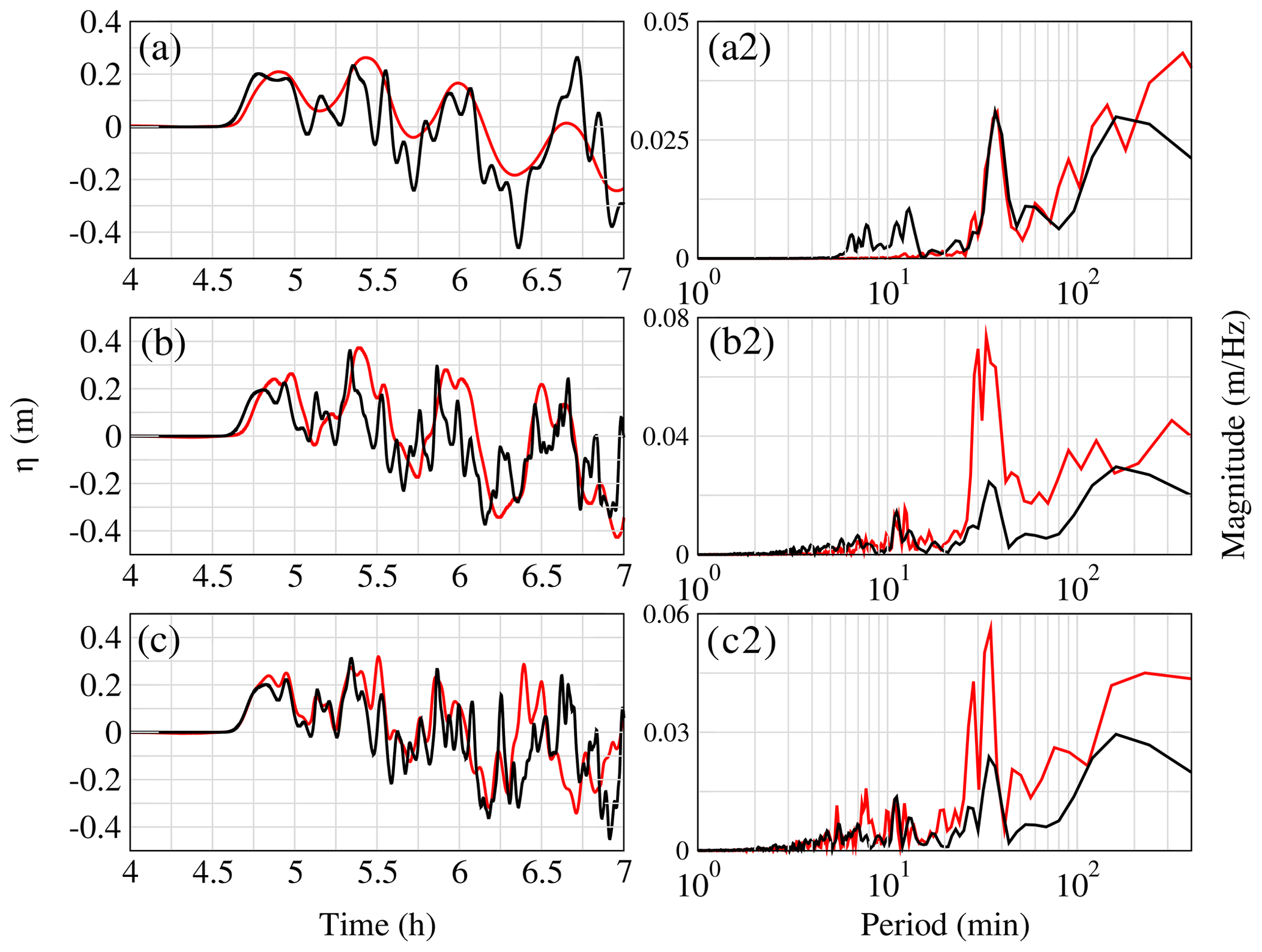
Figure 19 Comparison of the surface elevation (m) and the associated periods computed by a Fourier transformation (a2, b2 and c2) at Gauge 6 between Calypso (in black) and FUNWAVE-TVD (in red) for the 80 km³ scenario at the Gironde estuary for three resolutions: 2.7 km (a), 450 m (b) and 110 m (c) for FUNWAVE-TVD and 2 km (a), 500 m (b) and 125 m (c) for Calypso. The time takes into account the first 20 min of the slide and tsunami generation.

3.4 Comparison between FUNWAVE-TVD and Calypso

Figure 19 shows a comparison of the free surface signal computed at Gauge 6 by the reference model FUNWAVE-TVD and Calypso for different grids, i.e., (a) coarse grid only (Fig. 4) and nested computations (b) coarse + intermediate grid and (c) coarse + intermediate + fine grid (Figs. 4 and 5). We recall here that Calypso was run in Boussinesq mode on the coarsest grid and in shallow water mode (nondispersive) in the finer grids. The solutions computed by the two models on the finest resolution appear very similar at least for the three first waves (Fig. 19c). The comparison of panels (a), (b) and (c) gives an idea of the model convergence in the context of nested computations. On that particular point, the solutions computed by Calypso show less differences with grid resolution than FUNWAVE-TVD. For instance, the wave signal obtained with the intermediate grid is already close to the one obtained with the finest grid. This is not the case for FUNWAVE-TVD, which, with the coarsest grid, shows a wave signal with a clear cut in the high frequencies which is also visible in the spectra (Fig. 19a2).

3.5 Impact assessment

Figures 20 and 21 show the maximal simulated sea surface elevation for the 80 km³ scenario computed by FUNWAVE-TVD at an oceanic scale from the source to the studied areas. A gradual decrease in the maximum wave height due to radial attenuation can be observed, which is modulated by energy focusing in narrow directions as already pointed out in Løvholt et al. (2008).

Figure 20 Maximum surface elevations (m) computed by FUNWAVE-TVD for the 80 km³ scenario from the generation area to the French coasts and other remote territories at a 2.7 km resolution. The red rectangle represents a daughter grid covering the western French coasts (see Figs. 5 and 21).

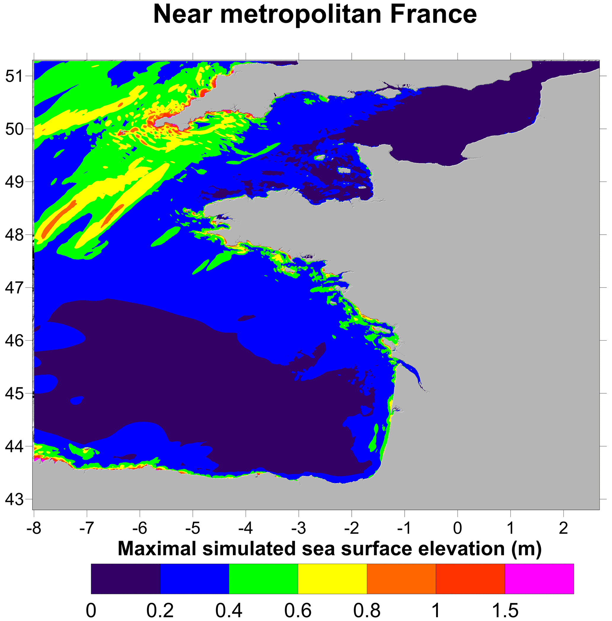
Figure 21 Maximum surface elevations (m) computed by FUNWAVE-TVD for the 80 km³ scenario on the western French coasts at a 450 m resolution.

Territories close to the generation area are highly affected. The first locations impacted are the other surrounded Canary Islands, nearby archipelagos (Madeira Island, Cape Verde) and west Africa, especially the western Sahara (Dakhla city – 100 000 inhabitants) and specific parts of Morocco through refraction on shallower part of the local bathymetry (Agadir, Essaouira and Safi – 800 000 inhabitants overall). In the latter areas, the waves are larger than 5 m.

The wave propagating toward Europe is obviously less energetic than in the western direction on which the main part of the energy is focused (Fig. 20). Nevertheless, Portugal, the western coast of Spain and, to a lesser extent, the southern coasts of Ireland and England are significantly affected. Lisbon, Porto, Vigo and Corunna appear to be the main cities at risk for the 80 km³ tsunami scenario with a surface elevation of about 2 m. When approaching the French Atlantic coastline (Fig. 21), the wave experiences shoaling on the continental shelf, and the wave height slightly increases. Even though France is less affected than the previous territories because the coasts are protected by the Iberian Peninsula, waves reach up to 1 m at various points located north of the Gironde estuary up to the northern part of the Brittany peninsula.

Figure 22 shows the distribution of the maximum surface elevations in the most refined domains of Calypso. A running average of 10 points has been applied to present more readable results. The flow depth at −5 m is on average 1 m in the Morbihan area with one specific location (latitude 47.3^∘ N) subjected to a large 3 m flow depth. In the Gironde estuary and Saint-Jean-de-Luz areas, the flow depths are less than 1 m except in the northern part of the Gironde estuary and the southern part of Saint-Jean-de-Luz where about a 1 m flow depth is found.

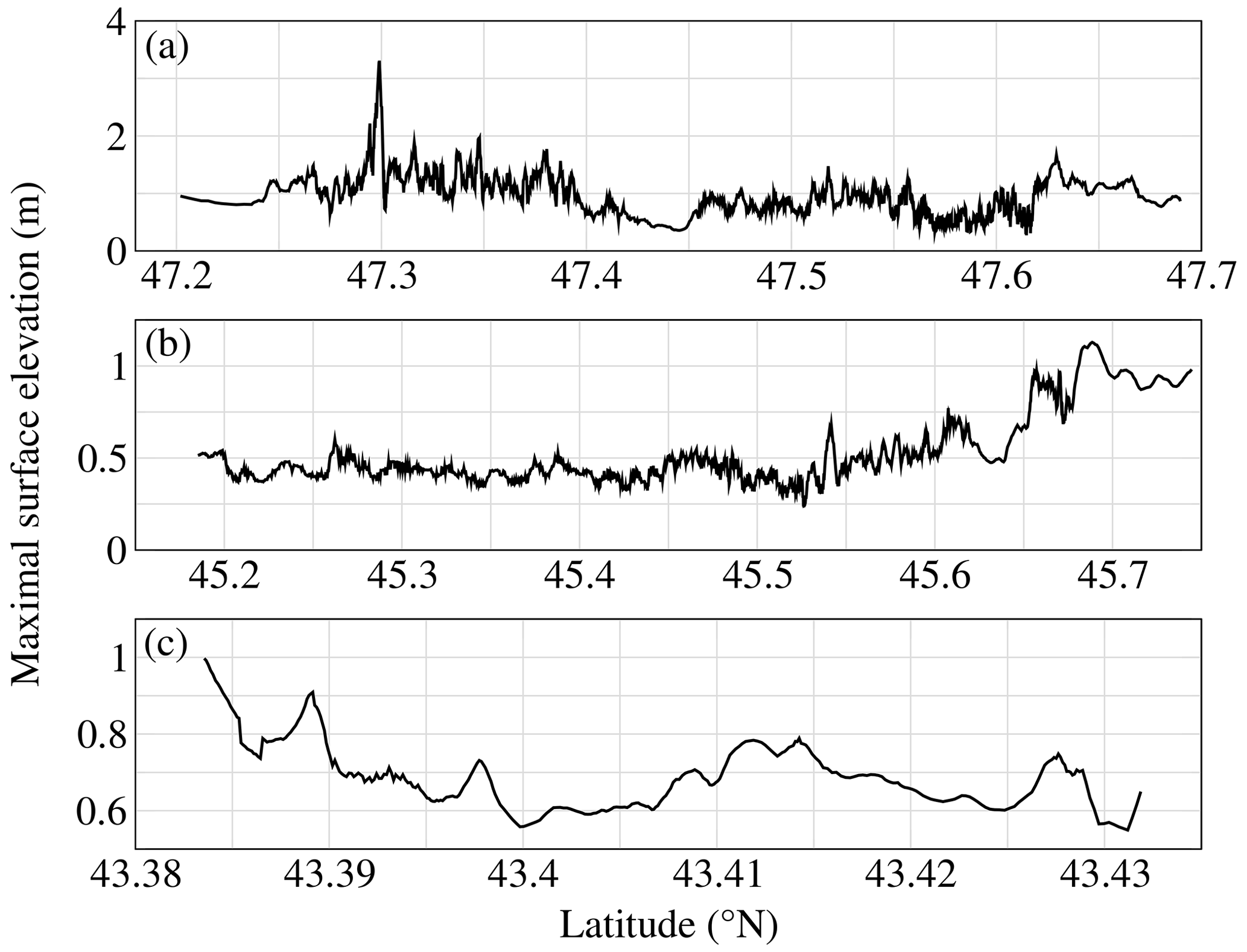
Figure 22 Maximum surface elevation computed with Calypso for the 80 km³ scenario using the finest grid resolution at isobath −5 m for different areas along the French Atlantic coastline: (a) Morbihan, (b) Gironde estuary and (c) Saint-Jean-de-Luz area

For the Guadeloupe archipelago, Fig. 23 shows the spatial distribution of the maximum surface elevation for the town of Sainte-Anne (Fig. 23a) and the town of Saint-François (Fig. 23b). The extent of inundation illustrates the potential dramatic consequences and the need for evacuation of town centers. Incoming waves may reach several meters at the shore line, threatening the fishery facilities of Sainte-Anne and the district of La Coulée in Saint-François. Urban areas are particularly exposed, such as Saint-François, Les Saintes, Sainte-Anne and Le Moule. As a consequence, the 80 km³ scenario should be considered a major tsunami with catastrophic consequences.

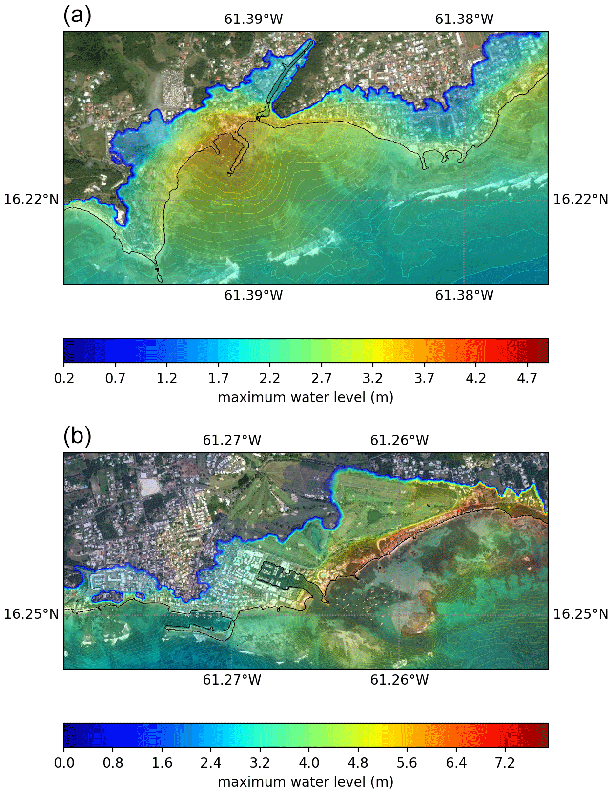
Figure 23 Flood map showing the maximum water level reached during the 80 km³ scenario for the region of Sainte-Anne (a) and Saint-François (b) (see locations in Fig. 6) computed by SCHISM. Map created using ArcGIS^® software by Esri. ArcGIS^® and ArcMap™ are the intellectual property of Esri and are used herein under license. Copyright © Esri. All rights reserved.

Regarding the 20 km³ scenario (inundation maps not shown here), the overall flooded surface would reach about 9 km²; therefore, this event should already be considered as an important tsunami event with an appropriate warning and the evacuation of beaches, the seafront and areas close to the shore. In the 40 km³ scenario (inundation maps not shown here), the flooded surface may reach 22 km², which would include potentially dense urban areas such as Saint François and Terre-de-Haut in Les Saintes.

4 Discussion

The main goal of the present study was to improve the state of the art for the potential La Palma tsunami source and to use this new proposed scenario to perform an impact assessment for Europe and, particularly, for French territories. Such high return period events with potentially catastrophic consequences are particularly important to study as accurately as possible since, due to the difficulty in assessing their precise return period, they often serve as a reference for hazard mitigation studies (Tehranirad et al., 2015).

The first result of the present work is the new tsunami source computed by Navier–Stokes simulation (for the initial 5 min), ad hoc filtering and Boussinesq wave propagation (for the following 15 min). As stressed previously, this source is more realistic than that considered in Abadie et al. (2012) due to the much larger viscosity used which is assumed to better approximate a granular slide. To support this, a comparison with existing granular experiments was performed, and the results extrapolated at real scale using a Froude–Reynolds similitude. Based on this new computation, we observed a significant diminution of the initial wave compared to the first assessment proposed in Abadie et al. (2012) (i.e., wave height approximately half that of the one previously computed after 10 min of propagation for the 80 km³ scenario). The new source (after filtering and propagation in the Boussinesq model) and comprehensive data on the slide are made available through the SEA scieNtific Open data Edition (SEANOE) portal (Abadie et al., 2019). These data allow potential users to either compute the slide on their own and do the whole sequence of computations or start from the already filtered wave solution to carry out propagation and impact studies.

The second result is a presumably better impact assessment in Europe generally and a new detailed impact assessment for France and Guadeloupe. Considering a credible yet extreme 80 km³ scenario, it is shown that the impact on the French Atlantic coast would remain moderate but could also be significant on the coast of Portugal and be very significant in the Guadeloupe archipelago. A direct comparison with Tehranirad et al. (2015) is difficult as the areas of interest were not the same in the two papers. Nevertheless, for instance, Tehranirad et al. (2015) found waves up to 10 m in the vicinity of the western Sahara and 5 m waves on the Portuguese coast, while they respectively reach 5 m and about 2 m in the present work, so the decrease is clear also far from the source.

Regarding the physics of the problem and the modeling strategy, the analysis of the wave signal obtained with FUNWAVE-TVD close to the source confirmed the presence of high frequency waves prone to dispersion at the depths encountered in this area of the Atlantic Ocean. Hence, physically, dispersion is expected, and, theoretically, an appropriate Boussinesq modeling is required. The results obtained with FUNWAVE-TVD appear consistent with what is physically expected: high frequency waves progressively disappearing from the spectra during the propagation. The comparison between FUNWAVE-TVD and Calypso, which showed good agreement, allowed us to simultaneously validate the models and secure the results obtained (even though some discrepancies remain in the low-frequency band). The methodology of performing transoceanic simulations in Boussinesq mode and shifting to NSW mode in the nearshore area is also validated through the good match observed in Fig. 19c. This figure also stresses the effect of resolution in tsunami propagation simulations. Indeed, such computations are generally CPU expensive, and the mesh is often adapted to this constraint, but Fig. 19 shows that the results largely vary with resolution. Therefore, convergence of the results is also a critical aspect to verify and demonstrate in order to obtain accurate results. In the present study, both Boussinesq models are found to converge approximately toward the same solution, which appears encouraging.

Of course there are some limitations in this study which may provide the basis for future improvements. First, this study should not be considered as a hazard assessment stricto sensu because the return period aspect is not considered, and the sensitivity in the landslide parameters is not covered extensively. For a review of probabilistic tsunami hazard analysis (PTHA) methods, the reader is referred to Grezio et al. (2017), for instance. Instead, the current study presents plausible particular scenarios based on state-of-the-art numerical models. Note that the Navier–Stokes model, which provides interesting information for those kinds of processes, is still too complex to be employed in PTHA computations.

Second, we used a glass-beads-based experiment (Viroulet et al., 2013) to calibrate the Navier–Stokes simulation of the La Palma slide. If this is an improvement compared to the very coarse inviscid initial estimation (Abadie et al., 2012), which should be considered as a worst case, such a laboratory experiment still is a huge simplification of the complexity expected in a real volcano collapse. An accurate description of such a complex process at real scale is still beyond the capabilities of current models. Therefore, there is here a very important source of uncertainty which the reader has to be aware of, and this uncertainty propagates and affects the impact results. Furthermore, this work is not a hazard study which could have been performed, for instance, by considering different values of slide viscosity but at a much higher computational cost. The position of this paper is rather to give an illustration of what could be expected from such an event by presenting results at least consistent with the current state of the art in terms of laboratory experiments and therefore to propose an improvement compared to the previous published results in that case.

The present work did not explicitly take into account the possibility of a retrogressive scenario. Whether the flank collapse occurs en masse or in successive stages is obviously crucial in terms of wave generation. In this study, we proposed several slide volume scenarios which can be used for a crude assessment of the wave reduction in case the collapse occurred as several separate events with no interactions between the successive slides (e.g., the 20 km³ scenario may give an idea of what would happen if an 80 km³ slide were to occur progressively or in sequence). The interactions could be left for future research even though field evidence tends to show that these collapses may have occurred as separate events (Wynn and Masson, 2003) rather than in an actual retrogressive way.

On the other hand, the extreme scenario of 450 km³ as studied in Ward and Day (2001), Løvholt et al. (2008), Abadie et al. (2012), and Tehranirad et al. (2015) has not been computed in the present. This extreme scenario, however, remains possible as evidenced by the volumes of the deep water deposits identified in Masson et al. (2002) around this archipelago. Nevertheless, we focused on the 80 km³ as it is consistent with the size of the deposits identified at the toe of the volcano, possibly corresponding to its last massive flank collapse (about 300 000 years ago).

5 Conclusions

The wave generated by a potential Cumbre Vieja volcano flank collapse and its impact on Europe and Guadeloupe was studied in this work. The source computation used an improved characterization of the slide rheology compared to previous works. Moreover, the subsequent propagation was performed using different models, which allows for a model comparison in a real configuration. The main conclusions of the work performed are the following.

• The new wave source is reduced by half compared to previous estimations mainly due to the larger value of slide viscosity used in this work.

• The wave impact is still very significant on nearby areas and on more remote coasts, such as Guadeloupe, located in the path of the maximum wave energy for the maximum slide volume considered here (i.e., 80 km³). Smaller slide volumes (i.e., 40 and 20 km³) would have more moderate impacts on these remote areas.

• In Europe, the impact may be considered as moderate to significant in the most exposed areas, such as some areas in Portugal and Spain, and weak to moderate along the French Atlantic coast.

• The tsunami source calculated in this paper after 15 min of propagation in FUNWAVE-TVD and proposed to the community in the SEA scieNtific Open data Edition (SEANOE) repository is dispersive, and therefore we recommend using appropriate models (e.g., Boussinesq models) to propagate further this source in future studies.

• The comparison of the Boussinesq models (i.e., FUNWAVE-TVD and Calypso) mutually validates the models in this particular case and secures the results obtained. This comparison also stresses the importance of model resolution and the possibility to turn off the dispersive terms in the model after a certain distance of propagation.