Fire Weather Index: the skill provided by the European Centre for Medium-Range Weather Forecasts ensemble prediction system

In the framework of the EU Copernicus programme, the European Centre for Medium-Range Weather Forecasts (ECMWF) on behalf of the Joint Research Centre (JRC) is forecasting daily fire weather indices using its medium-range ensemble prediction system. The use of weather forecasts in place of local observations can extend early warnings by up to 1–2 weeks, allowing for greater proactive coordination of resource-sharing and mobilization within and across countries. Using 1 year of pre-operational service in 2017 and the Fire Weather Index (FWI), here we assess the capability of the system globally and analyse in detail three major events in Chile, Portugal and California. The analysis shows that the skill provided by the ensemble forecast system extends to more than 10 d when compared to the use of mean climate, making a case for extending the forecast range to the sub-seasonal to seasonal timescale. However, accurate FWI prediction does not translate into accuracy in the forecast of fire activity globally. Indeed, when all fires detected in 2017 are considered, including agricultural- and human-induced burning, high FWI values only occur in 50 % of the cases and are limited to the Boreal regions. Nevertheless for very large events which were driven by weather conditions, FWI forecasts provide advance warning that could be instrumental in setting up management and containment strategies.

1 Introduction

The prediction of fire danger conditions allows fire management agencies to implement fire prevention, detection and pre-suppression action plans before fire damages occur. However, in many countries fire danger rating relies on observed weather data, which only allows for daily environmental monitoring of fire conditions (Taylor and Alexander, 2006). Even when this estimation is enhanced with the combined use of satellite data, such as hot spots for early fire detection and land cover and fuel conditions, it normally only provides 4 to 6 h warnings. By using forecast conditions from advanced numerical weather models, early warning could be extended by up to 1–2 weeks, allowing for greater coordination of resource-sharing and mobilization within and across countries. Due to the improved skills of weather forecasting, the use of numerical weather prediction offers a real opportunity to enhance early-warning capabilities (Roads et al., 2005; Mölders, 2008, 2010). In recent years institutions such as Natural Resources Canada (NRC) and the US National Oceanic and Atmospheric Administration (NOAA) have implemented regional fire danger forecasting systems based on their operational weather forecasts (Bedia et al., 2018). The Global Fire Early Warning System is also an international initiative, promoted by the Canadian Partnership for Wildland Fire Science and the United Nations Office for Disaster Risk Reduction, to provide fire danger forecasts up to 10 d ahead using the Canadian operational weather forecasting system (https://www.canadawildfire.org/globalwildfre-ews, last access: 26 August 2020). Parallel initiatives are promoted by the European Commission under the umbrella of the Copernicus Emergency Management Service (CEMS), namely the European Fire Forecast Information System (EFFIS, http://effis.jrc.ec.europa.eu/, last access: 26 August 2020) and its global counterpart the Global Wildfire Information System (GWIS, http://gwis.jrc.ec.europa.eu/, last access: 26 August 2020). Both systems principally rely on the Canadian Fire Weather Index (FWI; Van Wagner, 1974; Van Wagner and Pickett, 1985) to rate fire danger and on numerical weather predictions to provide forecasted fire danger information at the European and global levels (San-Miguel-Ayanz et al., 2002).

Systems such as the FWI detect dangerous weather conditions conducive to uncontrollable fires rather than modelling the probability of ignition and fire behaviours. The FWI (developed in Canada) is specifically calibrated to describe the fire behaviour in a jack pine stand (Pinus banksiana) typical of the Canadian forests. However, its simplicity of implementation has made it a popular choice in many countries, and it has been shown to perform reasonably well in ecosystems very dissimilar to the boreal forest (Di Giuseppe et al., 2016a; de Groot et al., 2007). The FWI calculation only relies on weather forcings, and no information on the actual vegetation status is taken into account. When weather forecasts are used in place of observations, uncertainties can be introduced. Sources of uncertainty can be (i) the limited knowledge of the initial state and (ii) the misrepresentation of physical processes. In the former case, errors are randomly distributed around the true state (Orrell et al., 2001); in the latter, errors produce systematic deviations from the true state. In both cases, errors in the weather forecast may be amplified or damped by non-linear transformations in the fire weather model (Erickson et al., 2018). Thus, for example, a dry bias in the model in a certain region will lead to the persistent prediction of higher fire danger values compared to what would be calculated using local observations.

Handling random errors in weather forecasts is traditionally done through the use of ensemble prediction systems, where several simulations are performed starting from slightly different initial conditions and model configurations (Molteni et al., 1996; Buizza et al., 1999). Given the expenses of running an ensemble system, these simulations are usually conducted at a lower resolution than a single deterministic run. The forecast is then interpreted as probabilistic rather than deterministic. While it has been shown that the probabilistic information contained in an ensemble prediction system might be difficult to interpret for end users (Pappenberger et al., 2013), ensembles can boost confidence in the decision process during emergency situations as a cost–loss analysis can be associated with the different scenarios (Cloke et al., 2017). Moreover, ensemble predictions can have more information value than the single deterministic simulation (Richardson, 2000; Zhu et al., 2002). Systematic biases, on the other hand, can be reduced by model improvements. For instance, appropriate post-processing (bias correction) of the atmospheric model (Piani et al., 2010; Di Giuseppe et al., 2013a, b) or post-processing of the sectoral application outputs (Raftery et al., 2005) can correct resolved processes and improve the final forecast skill.

Given the above considerations, in this paper we assess the performance of the fire danger forecasting system developed for the Copernicus Emergency Management Service by the European Centre for Medium-Range Weather Forecasts (ECMWF) to predict the FWI values where a comparison is performed against observed weather conditions. The system is also assessed in terms of its capability to mark high danger when an event actually occurred, looking at the probability of detection of fire during 1 year of operation in 2017. As the Fire Weather Index is the main index of this system, we concentrate on this model component.

2 Methods

2.1 FWI calculation

2.1.1 General concept

The Fire Weather Index system provides an indication of fire danger conditions as influenced by four weather parameters: temperature, relative humidity, precipitation and wind speed (Van Wagner, 1987). It models the moisture content of dead woody debris of different diameter classes lying on three fuel beds and from these indicates what the rate of fire spread and the fuel available for combustion would be. It also provides a general indicator of fire danger: the Fire Weather Index (FWI).

A comprehensive description of the FWI system, the interaction between the various components and how these are used in fire management can be found in Van Wagner (1987) and Wotton (2009). Abatzoglou et al. (2018) showed that the FWI exhibits strong correlative relationships to burned area across some non-arid ecoregions globally, albeit with only weaker relationships in climatically drier regions (shrubland), with a larger correlation found in the boreal and evergreen temperate forests of western North America. Also Bowman et al. (2017) highlighted how high FWI values are often associated with the most extreme fire activities recorded using Fire Radiative Power (FRP) observations. As an FWI has been shown to provide a good metric for quantifying fire danger globally, the proposed analysis of forecast skills will concentrate on this index (Di Giuseppe et al., 2016a; de Groot et al., 2007).

2.1.2 FWI forecast

For each day indices of the FWI rating system are calculated operationally at the ECMWF using real-time forecasts. A full description of the modelling components can be found in Di Giuseppe et al. (2016a). The high-resolution (HRES) and the ensemble prediction systems (ENS) provide weather forecasts which extend up to 10 d in the future. The atmospheric forcings have a temporal resolution of 3 h and a spatial resolution of 9 km for the high-resolution run and 18 km for the ensemble prediction simulations. While the HRES forecast is a single (deterministic) model integration, the ENS provides 51 realizations from perturbed initial conditions and different model physics (Buizza et al., 1999). These ENS forecasts are used to assess uncertainties in the prediction.

Figure 1 GFED4 regional classification and the three regions selected to showcase the fire forecast performances (California, Chile and Portugal). The black dots show the spatial distribution of weather stations from the SYNOP network which have at least 30 observations recorded at 12:00 LT in 2017.

A model integration at any nominal time simulates atmospheric conditions at a different local time, depending on the location. FWI calculations are usually performed at 12:00 local time (LT) because the model was calibrated using measurements at 12:00 LT against fire behaviour in the most active window (between 14:00–16:00 LT; Van Wagner, 1987). Therefore to produce a snapshot at 12:00 LT, a temporal and spatial collage of 24 h time model simulations is performed. Atmospheric fields are cut into 3-hourly time strips using the closest 3 h forecast outputs and then concatenated together so that the final field is representative of the conditions around 12:00 LT within the 3 h resolution available (see Di Giuseppe et al., 2016a, for more details). ECMWF implementation for the FWI is initialized once, starting from idealized conditions and following Wotton (2009) values. It also does not implement any overwintering, meaning that the moisture codes are not reset to zero during cold winter months.

2.1.3 FWI reference and benchmark

As many forestry agencies still rely on observed meteorological data to provide fire danger, a first assessment of the quality of the forecasted FWI will rely on the comparison with observations. Despite the fact that several meteorological observations are available through the Global Telecommunication System (GTS) SYNOP network, only a subgroup of stations have at least 30 d of recordings at 12:00 LT during 2017 (spatial coverage is given in Fig. 1). Many fire-prone regions, such as Australia, would not be covered by this comparison. In order to overcome this limitation, a reference dataset of FWI-modelled values is also used. This dataset is publicly available through the Copernicus Climate Data Store and is constructed using the ERA5 reanalysis dataset. ERA5 is the latest of ECMWF reanalysis products and was released at the beginning of 2019. It replaces the previous ERA-Interim database (Dee et al., 2011; Vitolo et al., 2019), providing a much improved spatial resolution and an extensive increment of assimilated observations. Simulations begin in 1979 and are updated in quasi real time with less than a week's delay. Fields have a spatial resolution of about 30 km and hourly time resolution. Outputs from ERA5 undergo the same temporal interpolation described in the previous section to provide the model with a composite fire reanalysis product at 12:00 LT. It has to be noted that, compared to local observations, a reanalysis provides a dynamically consistent estimate of the climate state at each time step and can, to a large extent, be considered a good proxy for observed meteorological conditions. Moreover, by combining different observations, reanalysis datasets extend well beyond the natural life of single observational networks, and they can provide a more homogeneous spatial coverage than using local observations. From ERA5 we also derive a climatological benchmark simulation (called CLIM hereafter). At the pixel level and for every day of the year, CLIM is constructed using 51 randomly sampled values (with replacements) from observed meteorological forcing in the period 1980–2019, excluding the verifying year (2017). CLIM has the advantage of having the same climatology of ERA5 but has no expected predictive skill. The advantage of CLIM is that in theory it has near-perfect reliability with regards to the ERA5 runs since it is produced with the same unbiased forcing data. It should, therefore, score better or equal to the forecast as a predictor for time ranges beyond their respective limits of predictability. CLIM is therefore used in this study as a benchmark to rank the expected improvements provided by a forecasting system. A full validation of the FWI database derived from ERA5 can be found in Vitolo et al. (2020).

2.2 Observed fire events

While national inventories of wildfire activities exist in many countries, they can be heterogeneous and lack the temporal span desirable for the validation of a fire danger system at the global scale. Satellite observations can supply a valid alternative, especially as they cover remote areas where in situ observations are sparse (Flannigan and Haar, 1986; Giglio et al., 2003; Schroeder et al., 2008). Daily maps of FRP (Kaufman et al., 2003; Wooster et al., 2005) have been available from the ECMWF since 2003 through the Global Fire Assimilation System (GFAS; Kaiser et al., 2012; Di Giuseppe et al., 2017, 2018). This dataset has been developed in the framework of the Copernicus Atmosphere Monitoring Services (CAMS) and uses observations from the MODIS sensors on board the Terra and Aqua platforms and assumptions on fire evolution to calculate a continuous record of active fires. The GFAS dataset integrates all available FRP observations available in a day over a regular 0.1^∘ grid. According to Wooster et al. (2005), this provides an indication of the cumulative dry mass available for burning, which can then be related to fire emissions. In this paper, the FRP products are only used as an observation of fire events. However, FRP values are ignored and only used to derive a mask of fire occurrence based on a minimum detection criteria: FRP > 0.5 W m⁻² (Kaiser et al., 2012). A “hit” is recorded if the fire forecast predicts fire danger above the 90th percentile of its historical values (provided by the ERA5 simulations) when a fire really occurred.

2.3 Score metrics

The performance of the fire forecasting systems to reproduce observed FWI values is assessed using deterministic and probabilistic scores. Both the SYNOP database and ERA5 are treated as a proxy for observations in the evaluation. To assess the quality of the forecasts, we use traditional deterministic skill scores such as the mean bias (MB) and the mean absolute error (MAE). For a probabilistic assessment, the continuous ranked probability score (CRPS) is also employed (Hersbach, 2000). These metrics are defined as

$$\begin{array}{}\text{(1)}& {\displaystyle }& {\displaystyle }\mathrm{MB}=\sum _{p=\mathrm{1}}^{\mathrm{cases}}\left[F_{\mathrm{HRES}}-O\right]\text{(2)}& {\displaystyle }& {\displaystyle }\mathrm{MAE}={\displaystyle \frac{\mathrm{1}}{\mathrm{cases}}}\sum _{p=\mathrm{1}}^{\mathrm{cases}}\sqrt{\left[{\left(F_{\mathrm{HRES}}-O\right)}^{\mathrm{2}}\right]}\text{(3)}& {\displaystyle }& {\displaystyle }\mathrm{CRPS}={\displaystyle \frac{\mathrm{1}}{\mathrm{cases}}}\sum _{t=\mathrm{1}}^{\mathrm{cases}}\underset{-inf}{\overset{+inf}{\int }}\left[F_n-O^{\mathrm{2}}\right]dn,\end{array}$$

where F is the forecast at time step t of N number of forecasts, and O is the observed value. While the MB and MAE are applied to a single forecast, the HRES forecast, the CRPS takes into account the whole distribution of possible values predicted by the ensemble. The CRPS is the continuous extension of the ranked probability score, where F_n is the cumulative distribution function of the predicted ensemble values. Then, the CRPS compares the cumulative probability distribution of the FWI forecast by the ensemble system to the observation. In this sense the CRPS is sensitive to the mean forecast biases as well as the spread of the ensemble (Hersbach, 2000).

While conventional skill score can be employed to assess the quality of the FWI computation, the verification of the FWI as a fire indicator is instead extremely challenging. First, as widely explained, the FWI is not a physical measure of fire activity but of its potential danger if one were ignited. Therefore high fire danger, while being correctly forecasted, might not result in active fires if there is no ignition and/or aggressive fire suppression. From the verification point of view, this means that the identification of false alarms is not meaningful, and the verification should mainly rely on hits and misses. Secondly, fires are rare events and, as for any other infrequent phenomena, the verification statistics are heavily influenced by the small number of hits when compared to the total. Still, when the cost of a missed event is high, for example in terms of human lives, the deliberate over-forecasting may be justified (Richardson, 2000; Cloke et al., 2017).

In these cases a positively oriented score such as “hit rate” may be useful, especially if related to the case of not having a forecast at all. Also, forecast quality does not always equal forecast value (Richardson, 2000). A forecast has high quality if it predicts the observed conditions well according to some objective or subjective criteria. It has value if it helps the user to make a better decision in terms of protective actions (Cloke et al., 2017). For example predicting high temperature and low precipitation in desert areas might be accurate but carries low information content and therefore limited value. Following these arguments and to gain an appreciation of the potential value of the forecasting system globally, we use as a metric the probability of detection (POD), which measures the fraction of the observed events that were correctly forecast: $\mathrm{POD}=\mathrm{hits}/(\mathrm{hits}+\mathrm{misses})$. Therefore, POD only takes into account observed fires and, unlike other skill scores such as the Brier score, does not suffer from artificial vanishing due to the high number of correct negative and false alarms (see Stephenson et al., 2008, and Ferro and Stephenson, 2011, for a discussion on this problem).

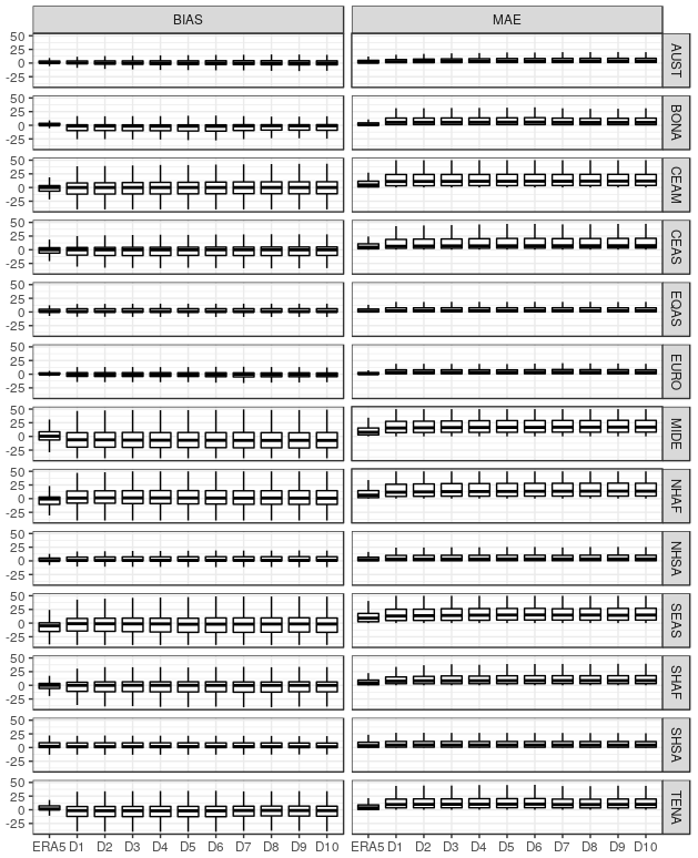
Figure 2 Comparison between modelled and observed FWI value across the GFED macro-regions. The FWI calculated using ECMWF high-resolution forecasts at different lead times is verified against ERA5 simulations. The box plots describe the distribution of values across the observation points for 1 year of simulations in 2017. Mean bias is plotted in the left panel and mean absolute error in the right panel.

2.4 Fire regions

The global assessment of the fire forecast skills is mostly provided as an average over selected regions even if the calculation of the various scores is performed at the pixel level by interpolating the model grid over the verification points. For an assessment at the continental scale, we use the fire macro-regions defined by the Global Fire Emission Database, GFED4 (Giglio et al., 2013). These macro-regions are characterized by different fire regimes and are very roughly homogeneous in their contribution of burning emissions (Giglio et al., 2013). Inside these regions we also select three areas at the national and regional level – California, Portugal and Chile – which experience recurrent intense fire episodes and saw major events taking place in 2017 (Table 1). Events in these locations are also analysed in detail.

Table 1 Event summary table.

3 Results

3.1 Skill in the FWI prediction

The first assessment looks at the capability of ECMWF fire forecasts to reproduce the same FWI values as would be estimated from the network of local stations but up to 10 d ahead. The selected stations (Fig. 1), which have at least 30 records during 2017 at 12:00 LT, are used to perform an analysis of MB and MAE at different lead times (Fig. 2). For comparison FWI calculations using ERA5 are also included, which provides a validation of the assumption that ERA5 is a good proxy for observations. As expected there is a performance degradation going towards longer lead times; however the increase is in within the distribution, and mean biases are limited to few units even on day 10. However caution is in order as, depending on the calibration procedure adopted, few units could mean a mismatch in danger level classification. The mean absolute error provides information on the residual amplitudes. The FWI from reanalysis has the sharpest skills, as expected, while the mean absolute error rapidly increases with lead times. However the distribution of MAE values clearly shows that in selected events the discrepancies between observed and predicted values are confined to few units even 10 d ahead. As it is recognized that in some regions in the tropical areas the number of stations is very reduced, a similar analysis is also performed using ERA5 as the verifying databases (see Fig. 5 in the following section), which, however, confirms the general conclusions.

Despite its importance, the analysis performed using the SYNOP network is pointwise and does not homogeneously cover all the regions where fires are relevant. Moreover, MB and MAE are based on high-resolution forecasts and do not provide information about the performance of the ensemble forecasting system as a whole. A global assessment of the performances of the system is provided by the comparison between the CRPS curves for the forecast and CLIM when both are scored against ERA5 in 2017 (Fig. 3). The CRPS calculated from the CLIM database provided a useful benchmark for the forecast as it defines the error above which the information content stored in the forecast would be equivalent to the information provided by the climate. The first interesting piece of information from comparing the two experiments is how far in advance there is skill in predicting fire danger from a weather forecast. In fact the interception between the CRPS curve from the forecast run and the CLIM run marks the overall length of the predictability windows, i.e where the system still provides skills above climatology. Encouragingly, if we look at the global average, the window of predictability is longer than the 10 d range provided here, which also suggests that there is scope for extending the prediction to the sub-seasonal and seasonal timescales. The discontinuity visible on day 6 is an artefact due to the change in temporal resolution in the ECMWF forecast. Up to day 6, forecasts are stored 3-hourly and only 6-hourly after this time step.

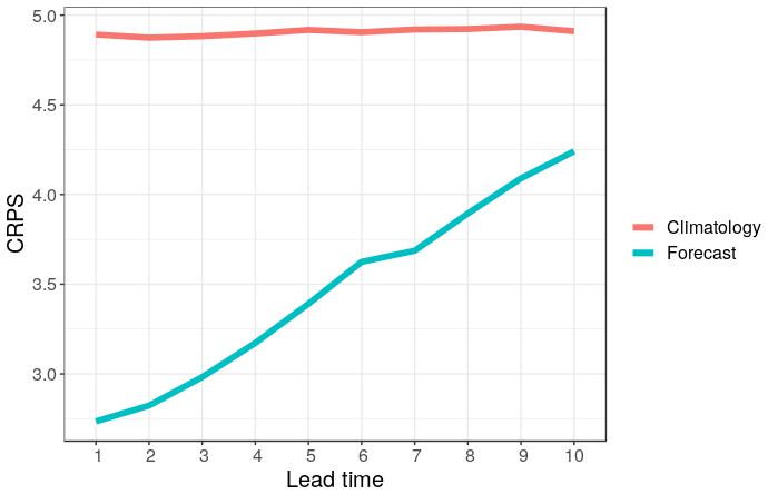
Figure 3 CRPS for the ensemble fire danger forecast (blue line) and the CLIM database constructed using a random selection of ERA5 years not including the verifying year (red line). Data have been globally aggregated and the forecast is available up to day 10 horizon.

There are some regional differences in the skill provided by the ensemble forecast. Regions covered by Boreal forests (e.g. BOAS, BONA, part of CEAS) have the largest predictability, with the maximum gaps between the forecast and the climate CRPS scores (Fig. 4). Savannah regions (NHAF, AUST, SHAF) tend to have a shorter window of predictability, with the forecast CRPS curve approaching at a shorter lead time than the CLIM ones. The regional differences in the prediction of the forecast FWI when compared to ERA5-derived databases are related to the skills of the forecast, which then project in the accuracy in the FWI simulation. While temperature prediction skills are globally mostly uniform, a complex picture emerges for the forecast skills of precipitation in all global models used for numerical weather prediction, including the ECMWF model. Prediction of precipitation at the mid-latitudes is notoriously more accurate than in the tropics due to the connection with frontal systems driven by large-scale dynamics (Simmons and Hollingsworth, 2002). Convective precipitation, which is the main source of rainfall in the tropics, occurs stochastically by nature and is therefore more challenging to predict. Although the gap has been filled through the years, forecast predictions in the southern extratropical region are less accurate than the equivalent in the Northern Hemisphere due to the availability of a better observing system to constrain the initial forecast conditions (Haiden et al., 2019). These considerations could largely explain the better performances of the FWI predictions in the Northern Hemisphere for the year taken into consideration. However it has to be noted that forecast skills have strong year-to-year variations, with expected increased skills in the tropic when large-scale phenomena such as the Madden–Julian Oscillation (MJO) and/or the El Niño Southern Oscillation (ENSO) take place. Under these phenomena the predictability of the tropics and of extratropical regions can substantially improve through teleconnections (Vitart, 2014).

Figure 4 As Fig. 3 but with aggregation performed on the GFED macro-regions.

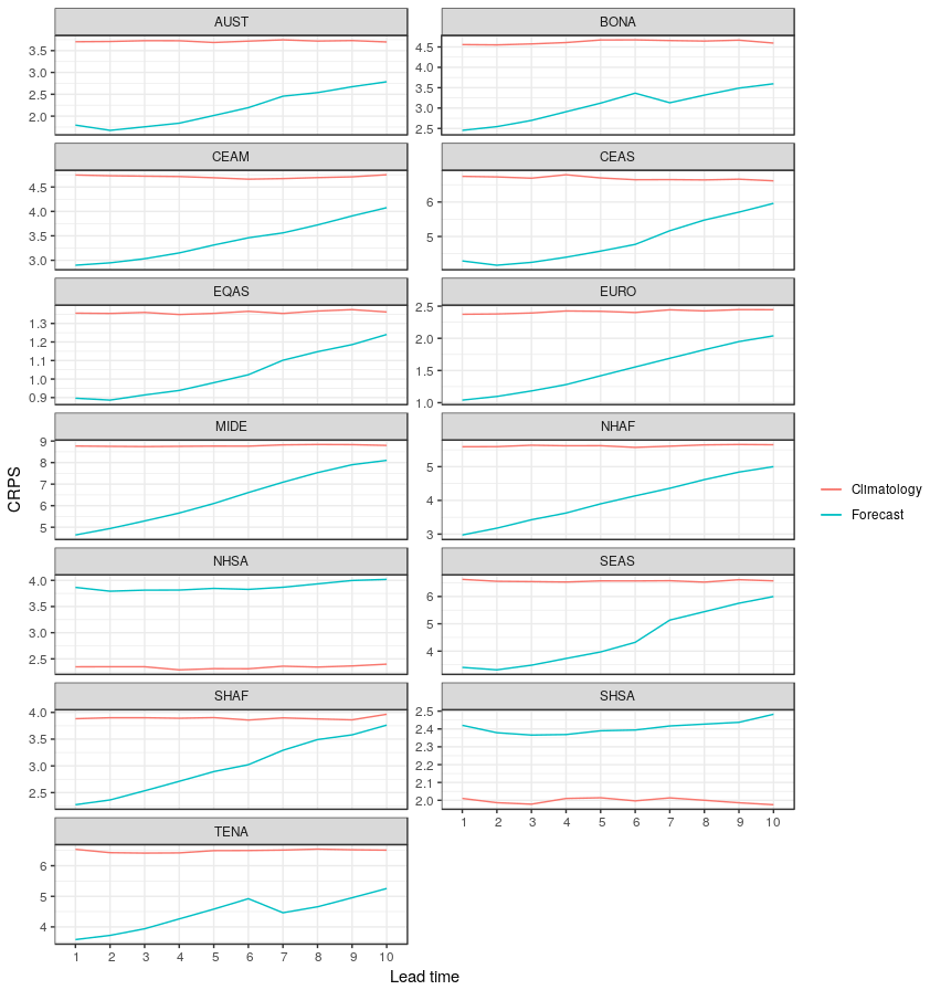
Exceptionally poor is the performance in the two South American regions, where the forecast at any lead time is below the climate line. As mentioned CRPS is heavily influenced by the forecast bias, which can induce a fast decline in the CRPS curve. Looking at the mean bias as a function of the lead time (Fig. 5), it is evident how these two regions are indeed strongly affected by systematic biases, with the largest values recorded at least in the first 3 d of forecasting. In general, for all the regions the decline in CRPS (Fig. 5) can, to some extent, be explained by the negative bias (too low FWI values when compared to ERA5-FWI). Interestingly the bias of the forecast is not spatially consistent; it is generally larger in the Southern Hemisphere regions and lower in the Northern Hemisphere, in agreement with what was discussed on the expected skills of the weather forecast. The consistent negative bias at all lead times also highlights that there is scope to improve the overall skill of the prediction through bias corrections of the meteorological forcing a (Piani et al., 2010; Di Giuseppe et al., 2013a, b).

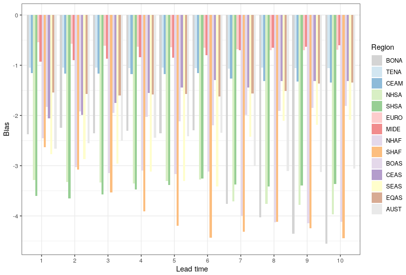
Figure 5 Mean forecast bias as a function of lead times and clustered by GFED macro-regions. The forecast bias for 2017 is assessed using the ensemble mean against the ERA5-based FWI database.

As a general conclusion and provided the possible year-to-year variability in skills, the general picture that emerges is that for most of the areas weather forecasting provides predictive skills for the FWI beyond 10 d.

3.2 Skill in detecting fire events

Being able to predict the observed value of the FWI does not equal to being able to pinpoint fires that occurred. Figure 6 shows the location of recorded fires in 2017 based of FRP observations from Moderate Resolution Imaging Spectroradiometer (MODIS) sensors as integrated by the GFAS platform (Kaiser et al., 2012; Di Giuseppe et al., 2016a, b). Fires covered large parts of the globe in 2017, with 157 631 cells recording FRP > 0.5 W m⁻². To understand the capability of the FWI to match the occurrence of actual fires, we assume that an active fire is correctly predicted if the FWI is greater than the 90th percentile of its distribution of values, here defined using the ERA5 database. Figure 7 shows a summary table of the mean probability of detection (POD) by region for all events in 2017 at forecast day 1 to 10. Given the intrinsic limitations of the POD as a skill metric, CLIM could provide a useful benchmark to understand the incremental skill provided by the forecast. The POD provided by CLIM was found to be below 0.1 in all regions and is therefore not shown in the table.

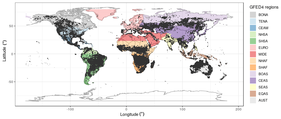
Figure 6 GFED4 micro-regions with the locations of all the 2017 events reported as active fires using the FRP observations from MODIS ingested into the GFAS system.

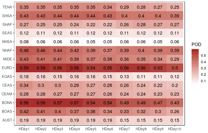
Figure 7 Regional probability of detection (POD) for the high-resolution forecasts from day 1 to 10 (HDAY1/10). Events where FRP ≥ 0.5 W m⁻² are categorized as “hits” and compared to the FWI prediction above the high warning level (90th percentile of climatology). The statistics are constructed using FRP observations detected in 2017.

CLIM has no skill in predicting fire events as it always provides the lowest POD, corresponding to a probability of detection below 10 %, even when compared to day 10 forecasts. On the other side, forecasts' POD varies widely by region, with Europe (EURO) and Boreal North America (BONA) being the only regions with POD above 0.5. These are mostly temperate regions where vegetation is dominated by forests and fuel is abundant and where fire danger is limited by moisture. In these regions the FWI is a good predictor of fire danger (Di Giuseppe et al., 2016a). It has to be noted that the FWI does not take into account management measures that could introduce a relevant number of “false alarms”. Central America, the Middle East and the areas of Africa in the Northern Hemisphere are characterized by a POD in the range of 0.2–0.5, as in most of the tropics, where fires usually occur in grasslands and shrublands. Here fuel is scarce and weather plays a less relevant controlling role. Also it has to be noted that the statistics here are likely to be contaminated by many agricultural and prescribed fires that are considered “events” and which would dilute some of the skill in regions where annual cropland is high or that are heavily managed.

One important exception is the very low performance of the fire forecast in equatorial Asia (EQAS) and South East Asia (SEAS), where the system seems to have a predictability below 0.2 (only 20 % of fires corresponded to the FWI above the 90th percentile). De Groot et al. (2007) highlighted how the FWI is not the best indicator in these areas, and a fire early-warning system should mostly rely on the drought code. There are a number of factors that could contribute to this low usability of the FWI in these areas. Fires in these regions are mainly caused by humans for the purposes of cleaning the land for establishing plantations (Field et al., 2009; Benedetti et al., 2016), and weather, which is the only driver of the FWI, is not the main fire trigger. However it has to be noted that 2017 was a very wet year in EQAS, and anomalously low FWI values were predicted (see for example Fig. 7 in Vitolo et al., 2020) with consistently low emissions recorded by the GFED. The low level for fire activities in 2017 means that the applicability of the results for this region in 2017 might not extend to other years with stronger activities. Also Australia (AUST) has a very low POD for the FWI, possibly being a fuel-limited ecosystem (Krawchuk et al., 2009). The main picture that emerges is that while weather forecast can provide skilful prediction for the FWI at least 10 d ahead, this fire danger index has in many areas a scarce capability to pinpoint emerging fires.

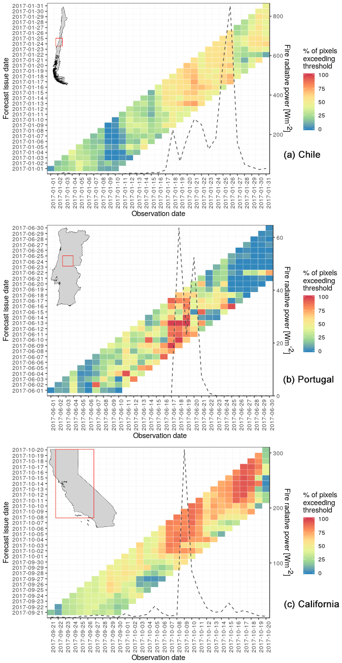
Figure 8 Comparison of FRP (dashed grey line with axis on the right-hand side) with the FWI forecasted using the deterministic high-resolution model for (a) Chile, (b) Portugal and (c) California. The FWI is colour-coded based on the percentage of pixels exceeding the high danger level calculated at the country and state level. Each of the panels refers to a specific fire event described in the text, and the statistics have been calculated over the red boxes.

3.3 2017 case studies

Figure 7 provides an averaged assessment of the global performances of the FWI to mark any fire pixels identified during 2017. This global statistic includes small fires and events that are not exclusively driven by weather conditions. FWI skill could improve locally, especial when important fire events are considered. It is important to understand how the information provided by a 10 d forecast could be used in real cases when the information is intended to aid emergency responses. Here we will analyse three cases of fire events that took place in 2017, which proved to be a year with extreme fire episodes across the globe. The 2017 wildfire season involved wildfires on multiple continents and also possibly unprecedented events when melted peat bogs ignited in Greenland. The year 2017 started with an extended fire in central Chile that lasted almost all of January. Strong winds, high temperatures and long-term drought conditions led to an event that has been described as the worst wildfire in Chilean history (Bowman et al., 2018). Fires in the central regions of O'Higgins, Maule and Bío Bío, south of Santiago, were difficult to control. Although fire activities had been recorded since July 2016, they became particularly intense in January 2017. In June, between day 17 and 18, another devastating fire hit Portugal. It claimed more than 60 lives, mostly recorded in the Pedrógão Grande area, 50 km southeast of Coimbra. A persistent heatwave had been building in the region, with temperatures above 40 ^∘C, which are highly unusual for the season. Moreover, relative humidity levels below 30 % had a role in the intensification of the deflagration and the spread of the wildfire, which raged out of control for several days (Boer et al., 2017). Finally in October, extensive wildfires raced just north of the San Francisco Bay area in California, causing historic levels of death and destruction. These so-called “Wine Country” wildfires were the most destructive in Californian history, with 44 deaths, the loss of 9000 buildings, damage to approximately 21 000 structures, USD 10 billion of insured losses and substantially greater total economic loss (Nauslar et al., 2018; Mass and Ovens, 2019).

Figure 8 shows the information that could have been provided for the study areas by the 10 d high-resolution (HRES) fire danger forecasts had these been already available. Each plot shows on the x axis the dates on which FRP was observed and, on the y axis, the dates forecasts were issued. The cell in the bottom-left corner shows the percentage of pixels in the study area that are expected to be above the 90th percentile of the FWI climatology for that pixel and day of the year. The forecasts for day 2 to day 10 are in the same row. The forecasts issued on the following day are one row above and so forth. The dashed lines show the observed FRP (see also secondary y axis).

The reader is reminded that active fires are triggered by highly unpredictable events (ignition) which are not accounted for in the FWI system. The FWI is not supposed to provide the exact localization of the event but an indication of potential fire activity. Large areas can be affected by anomalous conditions in the proximity of where the event really occurred. However it is encouraging that there is some capability for the forecast to detect the increase in fire danger associated with the three events even if with different intensities and sharpness. For the Chile case, for example, from mid-January around 70 % of the area often exceeded the high danger threshold. The FRP spike occurred on 26 January, and while the forecast was not able to capture this increase in fire activity, looking at the whole monthly sequence there is an indication of increased danger conditions even at 10 d lead time. However it is recognized that the signal extends for a long time and does not mark the peak of the fire activities. A much better timing of the event was instead forecast during the Portugal and California fires, which were very well predicted 10 d ahead.

4 Conclusions

In the last years, the ECMWF has been involved in the EFFIS development by providing weather forcing and fire danger calculations using its medium-range weather forecasts. Global fields of the FWI are calculated daily using the high-resolution (9 km) forecast up to 10 d ahead. The 18 km resolution ensemble prediction system provides 51 additional realizations based on slightly different initial conditions and/or using different model configurations (Molteni et al., 1996). These datasets are freely available in line with the data and information policy of the Copernicus programme, which intends to provide users with free, full and open access to environmental data. Using 1 year of preoperational service in 2017, we have showcased the potential of the use of weather forecasts to support the monitoring of fire danger conditions and planning in case of a potential emergency. Weather forecasting provides skilful information to derive FWI values up to 10 d ahead. Looking at the continuous ranked probability score for the forecast in comparison to climatological simulations, it was shown that predictive skills could also extend beyond the provided forecast range for most of the GFED macro-regions. Similarly to other sectoral applications (Wetterhall and Di Giuseppe, 2018), there is scope to extend the prediction to the sub-seasonal and seasonal (S2S) time frame. On the other hand a good skill in forecasting FWI values did not translate into a satisfactory probability of detection for real fire events. When all observed fires in 2017 were matched to high FWI values (>90th percentile), only the Boreal regions for which the FWI has been calibrated had a POD above 50 %. Mid- and high-latitude forested areas, where fuel is abundant, have the highest predictability, while in savanna/shrubland regions the relationship between the FWI and fire occurrence weakens. Still, global statistics are likely to be contaminated by many agricultural and prescribed fires that are considered “events” and which could dilute some of the skill in regions where annual cropland is high or that are heavily managed.

Looking at large fire events that occurred in 2017 in Chile, Portugal and California, we have shown that there are regional differences, and in Portugal and California the forecast was accurate up to 10 d ahead. Another interesting aspect attached to the use of weather forecasts is the use of probabilistic information. The quantification of forecast uncertainties through the use of ensemble predictions is something still pretty new in fire forecasting. However it opens great opportunities in terms of adding a confidence level to the fire prediction. These aspects will be investigated in follow-up work.