the Creative Commons Attribution 4.0 License.
the Creative Commons Attribution 4.0 License.
 | 06 Aug 2020
Evaluating the efficacy of bivariate extreme modelling approaches for multi-hazard scenarios
Bruce D. Malamud
Hugo Winter
Amélie Joly-Laugel
Modelling multiple hazard interrelations remains a challenge for practitioners. This article primarily focuses on the interrelations between pairs of hazards. The efficacy of six distinct bivariate extreme models is evaluated through their fitting capabilities to 60 synthetic datasets. The properties of the synthetic datasets (marginal distributions, tail dependence structure) are chosen to match bivariate time series of environmental variables. The six models are copulas (one non-parametric, one semi-parametric, four parametric). We build 60 distinct synthetic datasets based on different parameters of log-normal margins and two different copulas. The systematic framework developed contrasts the model strengths (model flexibility) and weaknesses (poorer fits to the data). We find that no one model fits our synthetic data for all parameters but rather a range of models depending on the characteristics of the data. To highlight the benefits of the systematic modelling framework developed, we consider the following environmental data: (i) daily precipitation and maximum wind gusts for 1971 to 2018 in London, UK, and (ii) daily mean temperature and wildfire numbers for 1980 to 2005 in Porto District, Portugal. In both cases there is good agreement in the estimation of bivariate return periods between models selected from the systematic framework developed in this study. Within this framework, we have explored a way to model multi-hazard events and identify the most efficient models for a given set of synthetic data and hazard sets.
Please read the corrigendum first before continuing.
-
Notice on corrigendum
The requested paper has a corresponding corrigendum published. Please read the corrigendum first before downloading the article.
-
Article
(10957 KB)
- Corrigendum
-
Supplement
(457 KB)
-
The requested paper has a corresponding corrigendum published. Please read the corrigendum first before downloading the article.
- Article
(10957 KB) - Full-text XML
- Corrigendum
-
Supplement
(457 KB) - BibTeX
- EndNote


A multi-hazard approach considers more than one hazard in a given place and the interrelations between these hazards (Gill and Malamud, 2014). Multi-hazard events have the potential to cause damage to infrastructure and people that may differ greatly from the associated risks posed by a single hazard (Terzi et al., 2019). Here, natural hazards (which we will also refer to as “hazards”) will be defined as a natural process or phenomenon that may have negative impacts on society (UNISDR, 2009). For modelling purposes, we consider two main mechanisms in natural hazard interrelations (Tilloy et al., 2019): (i) cascade interrelations (i.e. when there is a temporal order and causality between natural hazards) and (ii) compound interrelations (i.e. when several natural hazards are statistically dependent without causality).
Meteorological phenomena such as extratropical cyclones or convective storms often lead to the combination of multiple drivers and/or hazards and can therefore be related to compound events as defined by Zscheischler et al. (2018). This research concentrates on cascading and compound interrelations between natural hazards (e.g. a storm can include rain, lightning and hail, with rain and hail both potentially triggering landslides). Case examples of meteorological phenomena influencing natural hazard interrelations include the following:
- i.
In 2010, storm Xynthia hit the west coast of France. The storm itself was not particularly extreme for the season, but the compound effect of extreme wind, high tides, storm surges, extreme rainfall and the fact that the soils were already saturated led to huge damage due to wind and flooding (CCR, 2019).
- ii.
In summer 2010, Russia experienced a heatwave. Low precipitation in spring 2010 led to a summer drought that contributed to the heatwave having a large magnitude (Barriopedro et al., 2011; Hauser et al., 2015; Zscheischler et al., 2018). The co-occurrence of extremely dry and hot conditions resulted in widespread wildfires, which damaged crops and caused human mortality (Barriopedro et al., 2011).
- iii.
Extreme thunderstorms occurred in the Paris region in 2001, involving lightning and extreme rainfall, with the rainfall triggering flooding, mudslides and ground collapse, with subsequent damage to railway networks (CCR, 2019).
In this context, the quantification of interrelations between natural hazards can play an important role in risk mitigation and disaster risk reduction. Some of the natural hazards presented in the above examples are extreme occurrences of environmental variables (e.g. extreme temperature) which have different characteristics and statistical distributions (e.g. wind and landslides). Natural hazards can be interrelated with different mechanisms (i.e. compound, cascade). For a given mechanism, interrelations also vary in strength and intensity. Additionally, as highlighted in Tilloy et al. (2019), different modelling approaches have been developed to quantify interrelations between variables. Here we focus on stochastic models that include copulas (Nelsen, 2006; Genest and Favre, 2007; Salvadori et al., 2016) and multivariate extreme models (Heffernan and Tawn, 2004), limiting our analysis to the bivariate case. The potential for misinterpretation of the dependence structure of two variables clearly presents a problem when end users try to account for hazard interrelations.
We choose six distinct bivariate models able to handle different types of tail (extreme) dependence: one non-parametric (JT-KDE), one semi-parametric (Cond-Ex) and four different parametric copulas (Galambos, Gumbel, FGM, normal; see Sect. 2 and Table 2). The fitting capacities of each model are compared with the estimation of level curves. Level curves are extensively described in Sect. 2.3. However, these curves correspond to probabilities that can be related to compound and cascading hazard interrelations. Compound interrelations are represented with a joint probability, while cascading (sequential) interrelations are represented with conditional probabilities.
Examples of joint and conditional probabilities are given in Fig. 1. A joint probability is the probability of two events occurring together where both variables are extreme (also called AND probability; Fig. 1a), and a conditional probability is the probability of an event given that another has already occurred (Fig. 1b). Figure 1 illustrates the concepts of joint probability and conditional probability, with daily rainfall data from a high-resolution gridded dataset of daily meteorological observations over Europe (termed “E-OBS”; Cornes et al., 2018) and daily maximum wind gust data at Heathrow Airport provided by the Met Office (2019). A wind gust here is defined as the maximum value, over the observing cycle, of the 3 s running-average wind speed (WMO, 2019). These datasets and the interrelation between extreme rainfall and extreme wind are discussed in Sect. 4.1.

Figure 1Illustration of joint and conditional extremes with daily rainfall r (mm d−1) and daily maximum wind gust w (m s−1) data at Heathrow Airport for the period 1971–2018: (a) joint extremes (AND) of rainfall and wind gust (blue circles); (b) conditional extremes of rainfall given that wind gust is extreme (yellow circles). Daily rainfall data from E-OBS (Cornes et al., 2018) and daily maximum wind gust (3 s period) data from the Met Office (2019).
Joint and conditional probabilities are relevant metrics for practitioners and have been studied and used in several studies in the environmental sciences (e.g. Hao et al., 2017; Zscheischler and Seneviratne, 2017). However, as the most widely used level curve is the joint probability curve, we initially focus on it. To analyse our results and compare the performances of the models, we designed diagnostic tools that are presented in Sect. 3.2.
This paper is organized as follows. We first (Sect. 2) provide a theoretical background on key concepts used in this study and present the models and methodology used. We then (Sect. 3) discuss the characteristics of our synthetic dataset and present the results of the simulation study. The diagnostic tools used to compare models are also discussed (i.e. joint return level curves and dependence measure). As a result, a map exhibiting the strength and weaknesses of our six models is presented. It aims to provide objective criteria to justify the use of one model rather than another for a given set of hazards. Two applications to pairs of natural hazards that can impact energy infrastructure are presented in Sect. 4.
The main purpose of these data applications is to illustrate our methodology, but the natural hazard interrelations studied have the potential to negatively impact energy infrastructure. The first application looks at compound daily rainfall and wind in the United Kingdom. The combination of these two hazards can result in different and greater impacts than the addition of impacts due to extreme wind and extreme rainfall (e.g. wind destroys roof leading to greater damage, power plants flooded and rescuers slowed down by strong winds; Martius et al., 2016). The second application studies extreme hot temperatures and wildfires in Portugal. Extreme temperatures can lead to damage to infrastructure (e.g. rail track deformation) and put pressure on the energy infrastructure by increasing the demand (Hatvani-Kovacs et al., 2016; Vogel et al., 2020); they also increase the probability of wildfires (Witte et al., 2011; Perkins, 2015) which have the potential to cause fatalities and destroy infrastructure (Tedim et al., 2018). We finish (Sect. 5) with a discussion and conclusions.
We are interested in modelling interrelations between hazards in the extreme domain. This implies the use of methods and concepts coming from the broad area of extreme value theory (EVT). Amongst the six models compared in this study, four are directly linked to EVT (JT-KDE, Cond-Ex, Galambos, Gumbel). Extreme value theory has its roots in univariate studies (Coles, 2001) and has been extended to the multivariate framework (Pickands, 1981; Davison and Huser, 2015). A theoretical background on extreme value theory is given in Sect. S1.1 in the Supplement. In this study, we focus on modelling the dependence between two variables. Bivariate extreme value models developed within the statistical community (Resnick, 1987; Heffernan and Tawn, 2004; Cooley et al., 2019) have recently been used for environmental applications and therefore natural hazard interrelations (De Haan and De Ronde, 1998; Zheng et al., 2014; Sadegh et al., 2017). In order to reproduce the complexity and variety of natural hazard interrelations, we use 60 synthetic datasets to compare the fitting performances of the models. In these synthetics datasets we vary two main attributes of the bivariate datasets: the dependence structure and the marginal (individual) distributions. Of these 60 different synthetic datasets, 36 datasets have asymptotically dependent variables and 24 have asymptotically independent variables (see Sect. 2.1 for a definition of these two concepts).
In this section, we first present the two types of asymptotic behaviour in bivariate extreme value statistics – asymptotic dependence and asymptotic independence – and discuss different dependence measures for the estimation of the relationship between two variables (Sect. 2.1). The six bivariate models are then described (Sect. 2.2). Finally, we discuss the concept of the return level in the bivariate framework (Sect. 2.3).
2.1 Bivariate extreme dependence
2.1.1 Asymptotic dependence and asymptotic independence
Let X1, … , Xn be n different variables, with each variable a vector that can take on multiple values. Assume that these vectors are random and independent and identically distributed (i.i.d.). The asymptotic dependence implies that if one variable Xk for k ϵ (1, n) has values Xk that are large, it is possible for the other variables to take on values that are simultaneously extreme (Coles et al., 1999). One way to characterize extremal dependence structures is to split them into those with asymptotic dependence and those with asymptotic independence. In the bivariate case, for the (X1, X2) random pair with joint distribution G, the random variables X1 and X2 are asymptotically dependent if the following conditional probability (Heffernan, 2000)
Here X1>x are those values of variable X1 that are greater than a threshold x, the probability of both X1>x and X2>x is , and x* is the upper end point (maximum) of the common marginal distribution.
The variables X1 and X2 are asymptotically independent if (Heffernan, 2000)
where u is a high threshold. In practice, extremal dependence is often observed to weaken at high levels (i.e. as x→1), and it can happen that dependence between variables is observed in the body of the joint distribution but that the multivariate distribution is in fact in the max domain of attraction of independence (Davison and Huser, 2015).
Using models that take the assumption of asymptotic dependence (independence) in the case of asymptotically independent (dependent) variables can lead to a large overestimation (underestimation) of the probability of joint extreme events (Ledford and Tawn, 1996; Mazas and Hamm, 2017; Cooley et al., 2019). The multivariate extreme value and regular variation theories presented in Sect. S1.2 provide a rich theory for asymptotic dependence (De Haan and Resnick, 1977; Pickands, 1981) but are not able to distinguish between asymptotic independence and full independence.
2.1.2 Tail dependence measures
A popular method to analyse hazard interrelationships is to compute dependence measures (Zheng et al., 2013; Petroliagkis, 2018). Dependence measures aim to describe how two (or more) variables are correlated.
When focusing on the dependence in the tails or extreme part of distributions, linear or rank dependence measures might not be accurate and other coefficients appear more relevant (Hao and Singh, 2016). Dependence between variables in the joint tail domain has been widely studied in the statistics community (Coles and Tawn, 1991; Ledford and Tawn, 1997; Coles et al., 1999; Heffernan and Tawn, 2004; Zheng et al., 2014). As explained in Sect. 2.1.1, in the tails, two variables can be either asymptotically independent or asymptotically dependent; different diagnostics and coefficients previously developed are summarized in Heffernan (2000).
In this study, we use the following tail dependence measures:
-
the extremal dependence measures χ and introduced by Coles et al. (1999);
-
the coefficient of tail dependence η, introduced by Ledford and Tawn (1996).
These coefficients aim to measure the extremal dependence for bivariate random variables (X1, X2) and assume initially that (X1, X2) have a common marginal distribution. Coles et al. (1999) defined the extremal dependence measure as follows:
with x a sufficiently high threshold. A sufficiently high threshold x is a value that can be considered as extreme within a given distribution (corresponding to a high quantile); the value of the threshold depends on the marginal distribution. The extremal dependence measure χ(x) is the probability of one variable (X1 or X2) being extreme given the other is extreme (X2 or X1). This measure χ varies in the range [0, 1], where a value of χ=0 means that the two variables are asymptotically independent and χ=1 means that they are perfectly dependent. The extremal dependence measure χ is only suitable for asymptotic dependence. In the case of asymptotic independence (χ=0), Coles et al. (1999) introduced the measure which falls between the range [−1, 1], 1 being asymptotic independence. Ledford and Tawn (1996) defined their coefficient of tail dependence to be able to assess the strength of dependence between two asymptotically independent variables. They show that the joint survivor function for random variables (Z1, Z2) with common standard Fréchet margins can be expressed as (see Sect. S1.2)
with z a sufficiently high threshold in the standard Fréchet space. L(z) is a slowly varying function while z→∞, and η is the coefficient of tail dependence, lying in the range [0, 1]. Different values of each coefficient and their implications are summarized in Fig. 2. For large z, the three tail dependence measures presented above are related in the following way (Ledford and Tawn, 2003):
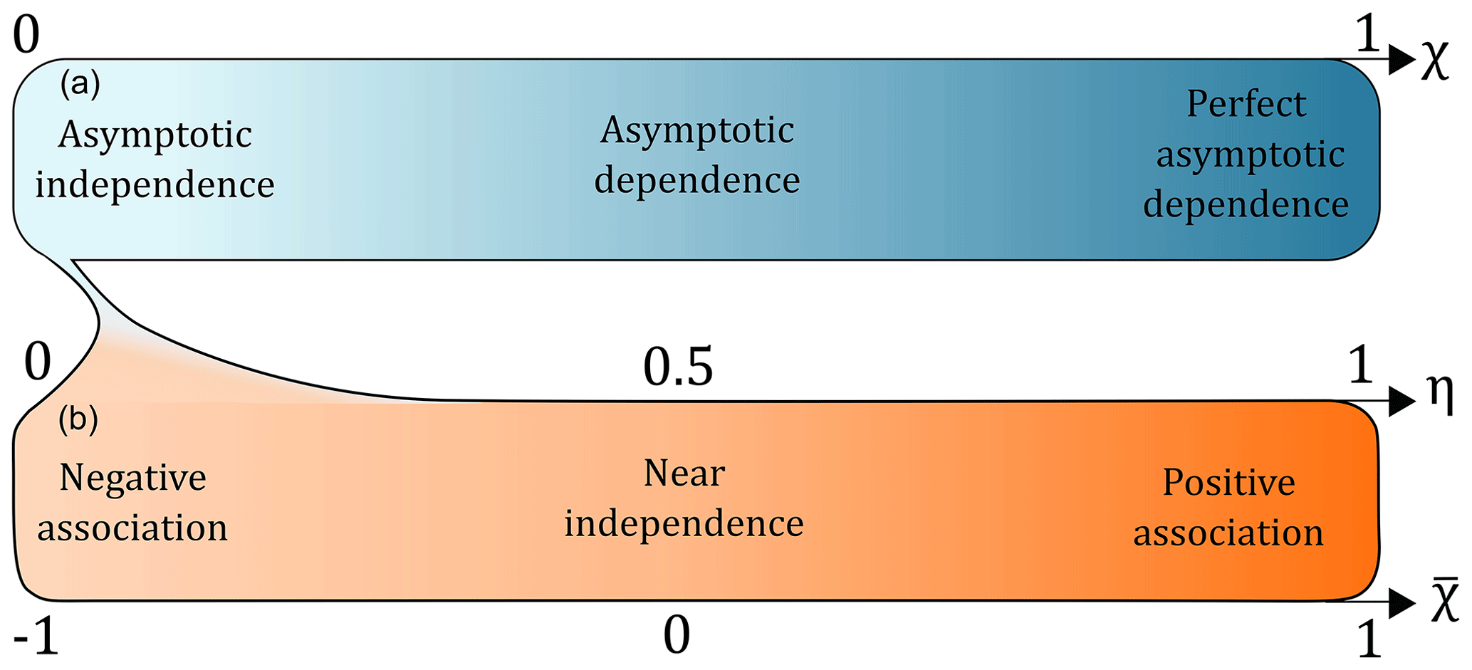
Figure 2The three coefficients used in this study to assess the dependence between two variables at an extreme level. In the upper part of the plot (blue), the coefficient χ varies between perfect asymptotic dependence (light blue; χ=0) and asymptotic independence (dark blue; χ=1). In the lower part of the plot (orange), which is in the asymptotic independence domain (in other words, χ=0) the coefficients and η both vary between negative association (light orange; ) and positive association (dark orange; ).
2.2 Bivariate models
Dependence measures are empirical measures which estimate the strength of the correlation or interdependence between two (or more) variables. Despite the fact that these measures provide crucial information, they do not allow for the modelling of joint (or conditional) exceedance probabilities. To model joint exceedance probabilities which represent the joint occurrence of hazards (here represented by extremes of environmental variables) in time and space, the use of stochastic models is required. In this section we present the three stochastic approaches for multivariate modelling that are used in the simulation study: parametric copulas, the semi-parametric conditional extremes model, and a non-parametric approach based on multivariate extreme value theory (see Sect. S1.2) and kernel density estimation.
2.2.1 Copulas
In the bivariate case, a copula is a joint distribution function which defines the dependence between two variables independently from the marginal distributions of these variables (Heffernan, 2000; Nelsen, 2006; Genest and Favre, 2007; Hao and Singh, 2016). Let the random variables (X1, X2) be vectors of i.i.d. values with marginal distributions F1(x1) and F2(x2) and a joint cumulative distribution function . Any bivariate distribution function with marginal distribution functions FX1(x1) and FX2(x2) can be expressed as a copula function as follows (Sklar, 1959; Nelsen, 2006):
where C is the copula function. Copulas are not limited to two variables, and Eq. (6) can be extended to higher dimensions. Several classes of copula with different properties are available, including Archimedean copulas and elliptical and extreme-value copulas (e.g. Joe, 1997; Nelsen, 2006). Extreme-value copulas have been used within various domains such as finance, insurance and hydrology because of their ability to model extremal dependence structures (Genest and Nešlehová, 2013).
However, extreme-value copulas are by definition asymptotically dependent as they follow the rules of multivariate extreme value theory (see Sect. S1.2). The two types of extremal dependence were presented in Sect. 2.1 and show that it is important to also consider asymptotic independence. Many copulas are asymptotically independent, including the normal copula and the Farlie–Gumbel–Morgenstern (FGM) copula (Heffernan, 2000). These two copulas will be used in the simulation analysis as asymptotically independent models (Sect. 3).
In the present study, the application of a copula model can be summarized in four main steps:
- i.
fitting marginal distributions to the two variables and then an empirical cumulative distribution function below a threshold and generalized Pareto distribution (GPD) above this threshold,
- ii.
transforming the variables to uniform margins – the transformed datasets no longer have information on the marginal distributions but keep the information about the dependence structure (Nelsen, 2006),
- iii.
fitting the copula function to the pseudo-observations by estimating the copula parameter(s) with an estimator (Genest and Favre, 2007),
- iv.
estimating the probability of joint events with the copula function previously fitted.
2.2.2 Conditional extremes model
The conditional extremes model (Heffernan and Tawn, 2004; Keef et al., 2013) is a semi-parametric model designed to overcome several limitations of copulas and other approaches such as the joint tail methods in which all variables must become large at the same rate. The aforementioned methods can typically handle only one form of extremal dependence, either asymptotic dependence or asymptotic independence. The conditional extremes model has the ability to be more flexible with asymptotic dependence classes; it can account for asymptotic independence and asymptotic dependence (Heffernan and Tawn, 2004; Keef et al., 2013). It can also be used to analyse more than two i.i.d. variables more easily than copula-based methods (Winter and Tawn, 2016); we restrict the theory provided here to the bivariate case. The conditional model has been used for different purposes: spatial or temporal dependence between extremes (Winter and Tawn, 2016; Winter et al., 2016), dependence between extreme hazards (Zheng et al., 2014) and even financial purposes (Hilal et al., 2011).
The conditional extremes model assesses the dependence structure between several variables conditional on one being extreme and aims to model the conditional distribution. As in joint tail models, the first step is to transform the marginal distributions; here the preferred marginal choice is Laplace (or Gumbel) margins (Heffernan and Tawn, 2004; Keef et al., 2013). Let the random variables (Y1, Y2) be vectors of i.i.d. values with Laplace distributions. The conditional extremes model aims to identify two normalizing functions a(yi) and b(yi) such that a satisfies and b satisfies . Both are defined such that for y>0 (Winter, 2016)
as u →∞, where G(z) is a non-degenerate distribution function. In the case of Laplace margins the normalizing functions a and b are given by (Winter, 2016)
where and . The different values of α and β characterize different forms of tail dependence. In the case where α=1 and β=0, variables (Y1, Y2) exhibit asymptotic positive dependence, and the case of asymptotic negative dependence is given when and β=0 (Winter, 2016).
Formally, the application of the conditional extremes model can be summarized in four main steps:
- i.
fitting marginal distributions to the two variables, an empirical cumulative distribution function below a threshold and generalized Pareto distribution (GPD) above this threshold;
- ii.
transforming those distributions onto Laplace (or Gumbel) margins;
- iii.
estimating the dependence parameters using non-linear regression;
- iv.
estimating the probability of joint events by simulating new extreme data through the conditional model.
2.2.3 Joint tail KDE (kernel density estimation) approach
The non-parametric approach used in this paper is an adaptation of the non-parametric approach presented by Cooley et al. (2019). Moreover, the dependence measures η is estimated to determine whether data are asymptotically dependent or asymptotically independent. This approach is based on the 2D kernel density estimator and the multivariate extreme value framework (see Sect. S1.2).
The kernel density estimation (KDE) method has the advantage of being a non-parametric way to estimate the joint distribution of n variables. With KDE, we make no assumption about the underlying distribution of the margins or about the dependence structure. The KDE centres a smooth kernel at each observation. The choice of the bandwidth is crucial when using this method (Duong, 2007; Hao and Singh, 2016). This selection was performed automatically in our case within the kernel survival function estimate from the R package “ks” (Duong, 2007, 2015).
The kernel density estimator is used here to estimate an empirical density distribution and a joint survival distribution of the bivariate dataset, where X=(X1, X2). The joint survival distribution corresponds to the joint exceedance probability of the two variables (see Sect. 2.3). From the joint survival distribution, it is possible to estimate level curves which are isolines corresponding to given joint probabilities of exceedance (see Sect. 2.3).
After estimating the joint survival distribution of the two variables with a kernel density estimator, the cumulative distributions of the two random variables are estimated empirically below a threshold and from a GPD above the threshold. The two marginal cumulative distribution functions are then transformed to Fréchet margins to allow the use of multivariate extreme value theory (Cooley et al., 2019):
Therefore, can be assumed to be regularly varying with an index of regular variation 1 (see Sect. S1). An extrapolation from a base probability pbase (blue area in Fig. 3) estimated with a kernel density to an objective probability pobj (purple area in Fig. 3) is then performed in the transformed space. Thus, on the transformed scale, it is possible to construct (Cooley et al., 2019). To produce level curves on the original scale, the transformation in Eq. (9) is reversed: . Figure 3 gives a graphical representation of the extrapolation performed within the joint tail KDE approach.
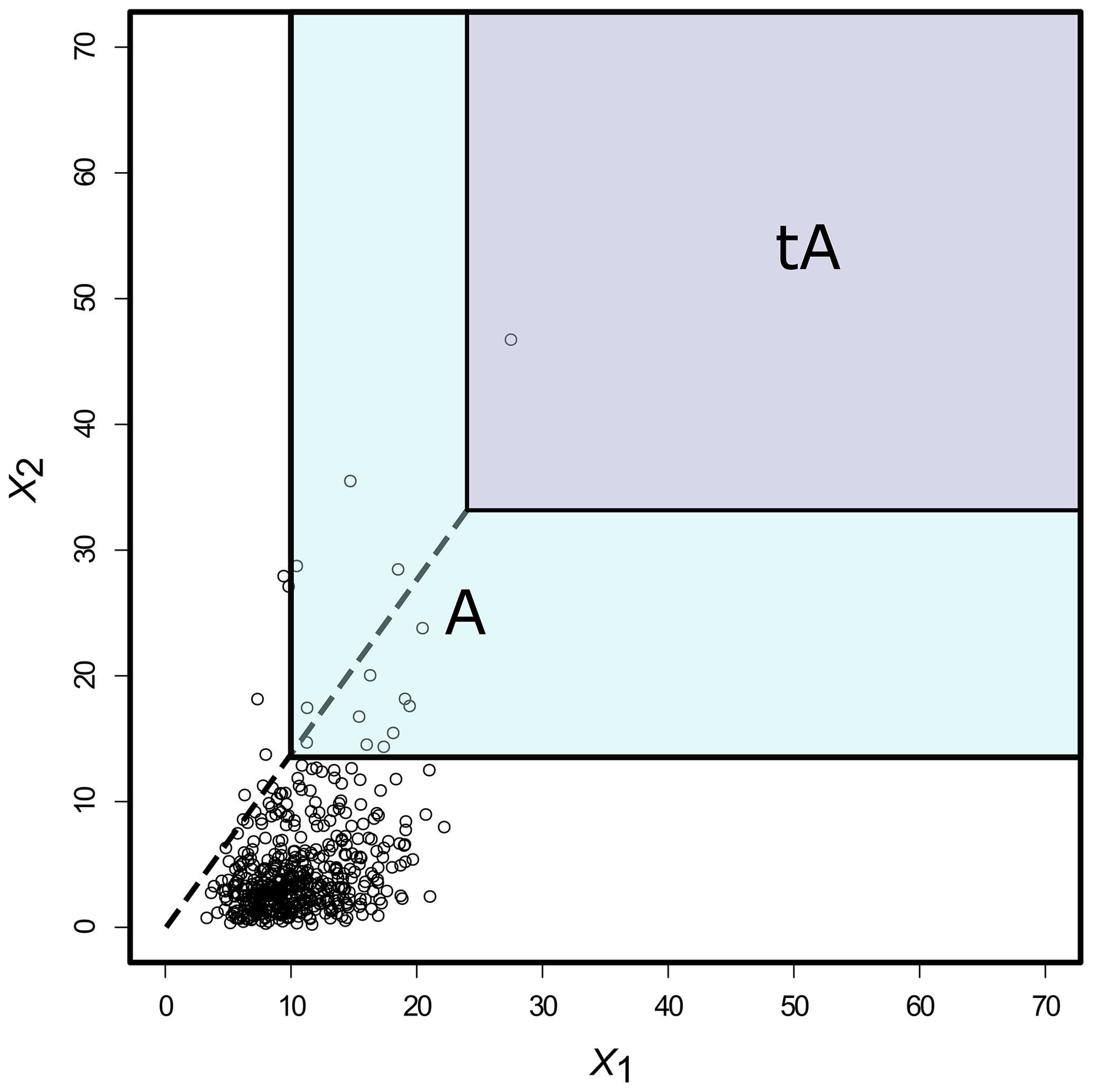
Figure 3Extrapolation in a regularly varying tail for a distribution in the max domain of attraction of some multivariate extreme value distributions. Black circles represent an asymptotically dependent bivariate dataset. In order to estimate the extreme joint probability P(tA) (where tA is an extreme set represented by the purple area), one can compute (where A is a less extreme set than tA, represented by the light blue area), with t<1. More data points are available in A than tA. Then, from the regular variation framework tP(tA)≈tP(A). Adapted from Huser (2013).
The methodology presented above is only valid when the two variables X1 and X2 are asymptotically dependent. In the asymptotic independence case, one needs to adjust the methodology. Two asymptotically independent variables follow the properties of hidden regular variation (Resnick, 2002; Maulik and Resnick, 2005; see Sect. S1.2.3). Formally, the coefficient of tail dependence η is introduced such that (Cooley et al., 2019)
The specificity of this approach (presented below) is that it combines a non-parametric estimation of the joint density and the framework of multivariate extreme values presented in Sect. S1.2. It can deal with both asymptotic dependence and independence. The coefficient of tail dependence estimation has an influence on the extrapolation process in the asymptotic independence case. Here we used the estimator presented in Winter (2016) which is derived from the joint tail model of Ledford and Tawn (1997).
Formally, the application of the joint tail KDE model can be summarized in five main steps:
- i.
estimating the joint cumulative distribution of the variables with a kernel density estimator,
- ii.
fitting marginal distributions to the two variables – empirical distribution below a threshold and generalized Pareto distribution (GPD) above this threshold,
- iii.
transforming those distributions into Fréchet margins,
- iv.
determining whether variables are asymptotically dependent or asymptotically independent by estimating the coefficients of tail dependence χ and η,
- v.
Estimating the probability of joint events and extrapolating the base isoline to an objective isoline.
2.3 Return levels in the bivariate framework
Studying natural hazards as multivariate – and particularly bivariate – events is a growing practice in multiple disciplines, including the following: coastal engineering (Hawkes et al., 2002; Mazas and Hamm, 2017), climatology (Hao et al., 2017, 2018; Zscheischler and Seneviratne, 2017) and hydrology (Zheng et al., 2014; Hao and Singh, 2016). There has been debate among scientists trying to define a “multivariate return period” (Serinaldi, 2015; Gouldby et al., 2017). Serinaldi (2015) defined seven different types of probabilities that can be considered as bivariate probabilities of exceedance. These can be expressed through copula notation.
Let the random variables (X1, X2) be vectors of i.i.d. values with marginal distributions Fi(xi), with , C their copula function (Sect. 2.3.1) and , where F1, 2 is the bivariate distribution function of X1 and X2, and u=F1 and v=F2 are standard uniform random variables. The seven types of probability and their equations are given in Table 1.
Table 1Types of probabilities for bivariate (X, Y) return period estimation. u and v are extreme thresholds. From Serinaldi (2015).
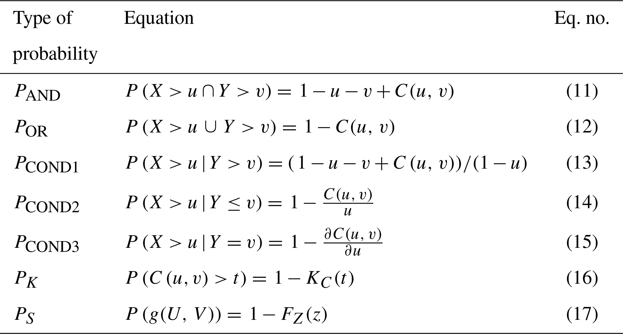
The function KC in Eq. (16) is the Kendall function and represents the distribution function of the copula (Salvadori and De Michele, 2010; Serinaldi, 2015). Equation (17) refers to the “structure-based” return period introduced by Volpi and Fiori (2012). Among these seven types of probabilities, we selected the “AND” and the “COND1” probabilities (see Fig. 4) as these are commonly used in the literature (Chebana and Ouarda, 2011; Tencer et al., 2014; Sadegh et al., 2018) and correspond to the two types of interrelations we are interested in (i.e. compound and cascade).
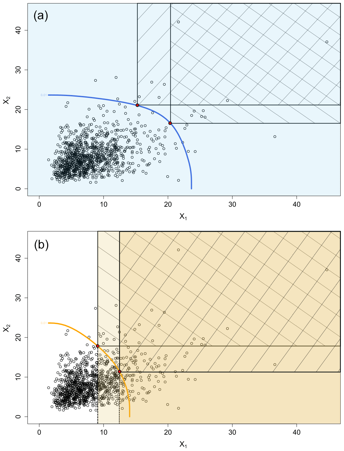
Figure 4Graphical representation of two bivariate (X1, X2) probabilities of exceedance: (a) PAND probability and (b) PCOND probability, with level curves (blue in a and orange in b) representing p=0.01 (1000 data points on a Gumbel copula with log-normal marginal distributions). Colours represent the domain on which the probabilities are computed while the areas with diagonal hatching represent the critical regions which are the regions corresponding to the given probabilities.
In 2D space, probabilities of exceedance (or quantiles) are not represented by a single value but by a curve with an infinite number of points with the same probability of exceedance. However, as shown in Fig. 4, these probabilities are defined by (i) the domain where these are computed and (ii) the critical region corresponding to the probability type. For the AND probability, the computation domain remains similar when moving along the curve while the critical region evolves constantly. For the COND1 probability, both computation domain and critical region evolve when moving along the curve (see Fig. 4). Bivariate probabilities of exceedance are curves. These curves have been given various names in different research papers including the following:
-
isolines (Salvadori, 2004; De Michele et al., 2007; Salvadori et al., 2016; Sadegh et al., 2017, 2018)
-
level curves (Coles, 2001; Salvadori, 2004; De Michele et al., 2007; Volpi and Fiori, 2012; Serinaldi, 2015, 2016; Bevacqua et al., 2017).
For the specific case of the AND probability, the following names have been used:
-
joint exceedance curves (Hawkes et al., 2002; Hawkes, 2008; Mazas and Hamm, 2017)
-
quantile curves (De Haan and De Ronde, 1998; Chebana and Ouarda, 2011).
Here we are interested in comparing the abilities of six different models presented in Sect. 2.3 to reproduce a given dependence structure. We create 60 different synthetic dataset types with varying marginal distributions and dependence structures. By doing this, we aim to produce bivariate synthetic datasets comparable to the ones studied in bivariate hazard analysis (Zheng et al., 2014; Hendry et al., 2019). This will allow us to confront the six models against the synthetic datasets, as a reference for bivariate hazard interrelation analysis (see Sect. 4). The six models compared in this simulation study are
- i.
the conditional extremes model (Cond-Ex; Sect. 2.3.2),
- ii.
the non-parametric joint tail model (JT-KDE; Sect. 2.3.3),
- iii.
the Gumbel copula (Gumcop; Sect. 2.3.1),
- iv.
the normal copula (Normalcop; Sect. 2.3.1),
- v.
the Farlie–Gumbel–Morgenstern (FGMcop) copula (Sect. 2.3.1),
- vi.
the Galambos copula (Galamboscop; Sect. 2.3.1).
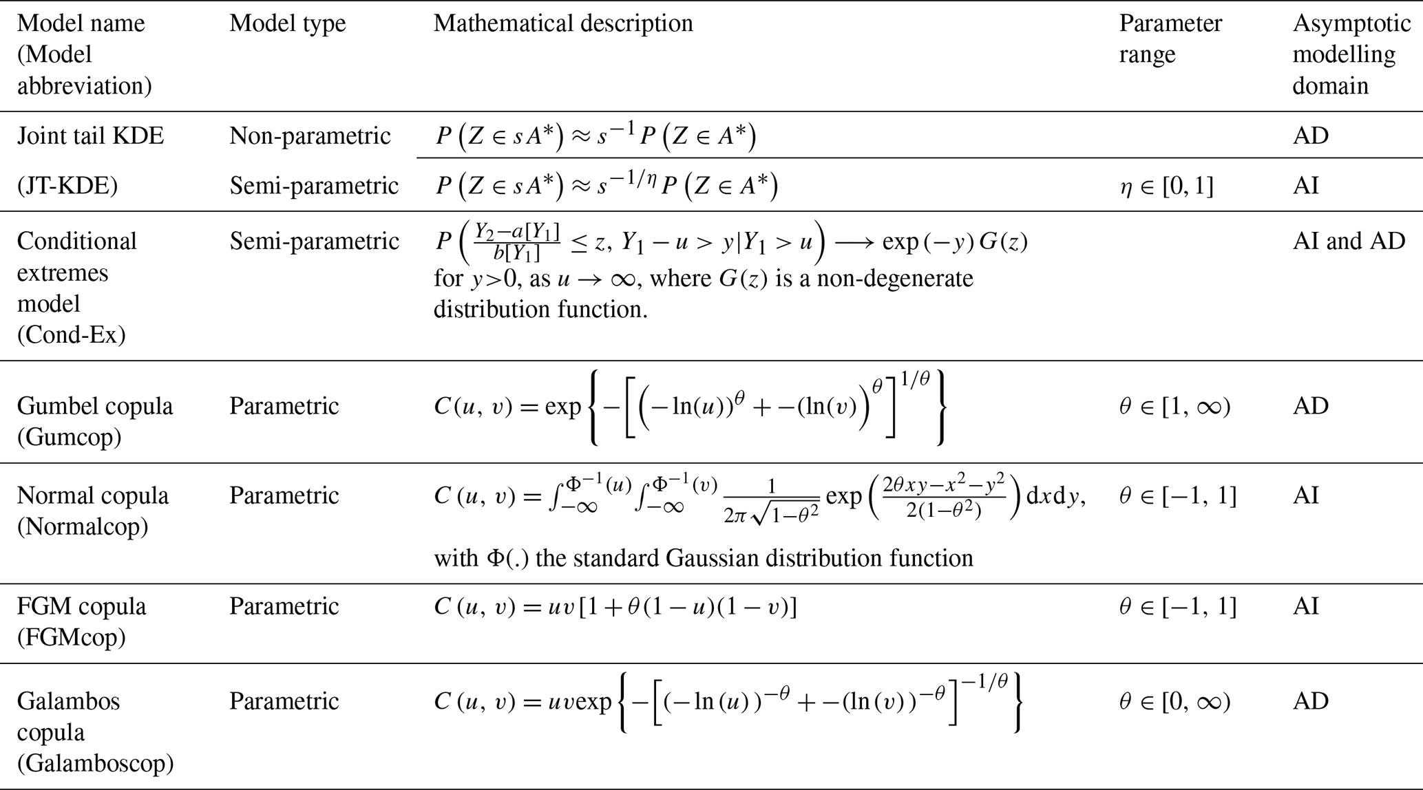
Among the four copulas used here, two are asymptotically dependent (Gumbel and Galambos) and two are asymptotically independent (normal and FGM). A description of the six models is given in Table 2. Table 2 synthesizes a range of information about all the six models used in this simulation study including their type (non-parametric, semi-parametric, parametric), equation, parameter range (if there is a parameter) and asymptotic modelling domain. This latter information is important to interpret the result of the simulation study in Sect. 3.3.
Table 2Description of the six statistical models compared in this article. The description includes the model name and abbreviation (used throughout the article), type of model (parametric, semi-parametric, non-parametric), the mathematical description, the parameter range (where relevant) and the asymptotic modelling domain (AI for asymptotic independence and AD for asymptotic dependence).
In this section, we first describe and display the synthetic data that have been generated to conduct this study. We shall then present the measures used in this study to compare the level curves and the dependence measures estimated from the six models presented in Table 2. Finally, results of the simulation will be displayed and analysed.
3.1 Synthetic data
Synthetic datasets are often used to compare different statistical models (Chebana and Ouarda, 2011; Zheng et al., 2014; Cooley et al., 2019). Here we generated 60 bivariate synthetic datasets representative of environmental data such as daily rainfall, daily wind gust and daily wildfire occurrences (see Sect. 4). The number of synthetic data points we use here has been fixed to 5000 for each dataset. For the asymptotic dependence case, 36 distinct datasets are generated from a Gumbel copula (see Sect. S1.3.1); for the asymptotic independence case, 24 datasets are generated from a normal copula (see Sect. S1.3.2). Each synthetic dataset set of parameters has been used to generate 100 realizations to produce confidence intervals.
The synthetic datasets are generated from two marginal distributions and a dependence model (i.e. copula). Both marginal distributions are log-normal; the log-normal distribution has been used (among others) for the modelling of a wide range of natural hazards, including wind, flood and rainfall (Malamud and Turcotte, 2006; Clare et al., 2016; Loukatou et al., 2018; Nguyen Sinh et al., 2019).
Random variables X with a log-normal distribution are governed by two parameters: the location parameter μ and the shape parameter σ, which correspond respectively to the mean and the standard deviation of Y, the variable's natural logarithm, i.e. Y=ln (X) (Aitchison, 1957). The parameter σ influences the shape of the distribution and the heaviness of the tail, and the dispersion of a log-normal distribution mostly depends on the shape parameter (Koopmans et al., 1964)
We can characterize log-normal distributions with the coefficient of variation cv which is the ratio of the standard deviation s of the log-normally distributed variable x to its non-zero mean (Malamud and Turcotte, 1999):
The standard deviation s and the non-zero mean are both related to the two parameters μ and σ of the log-normal distribution (see Table 3). The use of the coefficient of variation characterizes the log-normal distribution with one single parameter instead of two. The distribution used in the simulation study, the parameters, and the relationship between these parameters and the different tail dependence measures are summarized in Table 3.
Table 3Marginal distributions and copula used for the synthetic datasets.
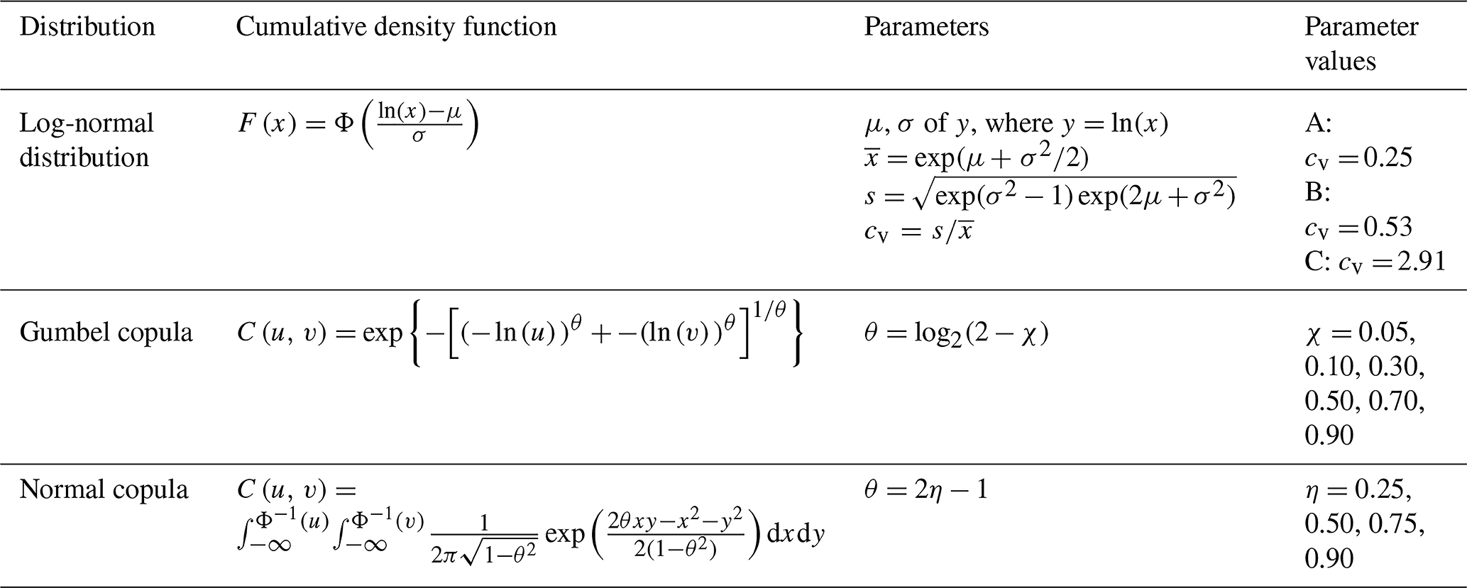
where Φ is the cumulative distribution function of the standard normal distribution.
We use three different coefficients of variations cv=0.25 (labelled as A for the rest of this paper), 0.53 (labelled B) and 2.91 (labelled C; see Table 3). The log-normal distribution A (cv=0.25) produces a distribution close to the normal distribution. The distribution C (cv=2.91) is a highly right-skewed distribution. The distribution B (cv=0.53) has intermediate skewness between A and B. In the bivariate context, there are six possible combinations of these distributions: AA, AB, AC, BB, BC and CC.
The dependence structure is represented by a Gumbel copula in the case of asymptotic dependence (AD) and a normal copula in the case of asymptotic independence (AI) as no copula can be both asymptotically independent and asymptotically dependent (Heffernan, 2000; Coles, 2001). The Gumbel copula is an extreme-value copula that is asymptotically dependent (see Eq. S19). The Gumbel copula function only has one parameter θ which can be related to the extremal dependence measure χ. Here, we vary χ between 0.05 (very weak asymptotic dependence) and 0.9 (strong asymptotic dependence; see Fig. 5). The normal (or Gaussian) copula is asymptotically independent. Its unique parameter is related to the coefficient of tail dependence η (Heffernan, 2000). We vary η from η=0.25 (negative subasymptotic dependence) to η=0.9 (positive subasymptotic dependence; see Fig. 5). In total, 10 different dependence structures were simulated for each of the six combinations of marginal distributions. The 60 bivariate synthetic datasets used in this study are displayed in Fig. 5.
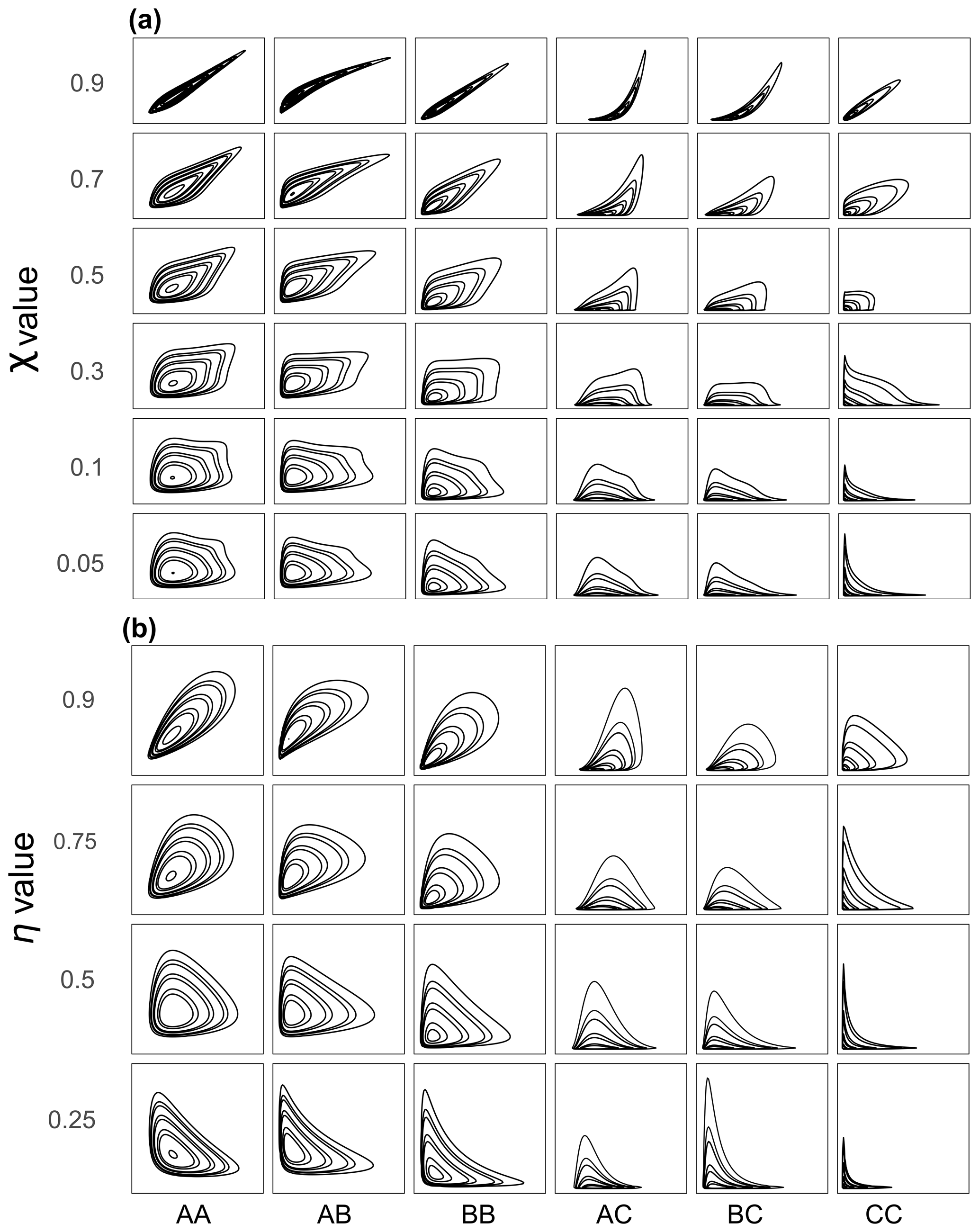
Figure 5The 60 different synthetic bivariate datasets used in our simulation study. On the y axis: the dependence strengths (a) χ (for asymptotic dependence) and (b) η (for asymptotic independence) vary from slightly negative association to heavily dependent (see also Fig. 2). On the x axis AA to CC represent the marginal distributions that are part of the bivariate distributions (see Table 3) with A, B and C representing log-normal distributions with different coefficient of variations cv (A: cv=0.25; B: cv=0.47; C: cv=0.95).
To compare the fitting capabilities of the different models presented in Sect. 2.3, we vary several characteristics of the synthetic dataset:
- i.
The shape of the marginal distributions. Natural hazards can exhibit very diverse statistical properties depending not only on their type but also on the location where they occur (Sachs et al., 2012).
- ii.
The strength of the dependence represented by the parameter of the copula function. The type and strength of the relationship between natural hazards can vary within a broad range depending on the natural hazard studied or the location (Gill and Malamud, 2014; Martius et al., 2016). In order to take into consideration both the AD and AI cases, the two parameters χ and η (Sect. 2.2) are used.
3.2 Diagnostic tools
There are many diagnostic tools to assess the goodness of fit of parametric bivariate models (Arnold and Emerson, 2011; Couasnon et al., 2018; Genest et al., 2009, 2011; Genest and Nešlehová, 2013; Sadegh et al., 2017). Amongst these, some of the most popular are the following:
-
Cramér–von Mises statistic (Arnold and Emerson, 2011)
-
Kolmogorov–Smirnov test (Arnold and Emerson, 2011)
-
Akaike information criterion (AIC; Akaike, 1974)
-
Bayesian information criterion (BIC; Schwarz, 1978).
These measures have been developed in a univariate framework and then extended to the bivariate framework. Genest et al. (2009) proposed several approaches for Cramér–von Mises and Kolmogorov–Smirnov goodness-of-fit tests for copulas. There are two issues we faced using these measures for our study:
-
These criteria are designed to fit on the dependence structure of the whole dataset and not on the extreme dependence structure which can be different.
-
In our study we aim to compare parametric and non-parametric models.
To tackle the first issue, goodness-of-fit tests have been developed for extreme-value copulas (Genest et al., 2011). The latter issue is more complicated; each modelling approach has its own fitting methodologies, and although it is now possible to compare copulas against each other (Sadegh et al., 2017; Couasnon et al., 2018), it is more difficult to compare copulas against semi-parametric or non-parametric models. The measures mentioned above are not suitable for the present study as they require models to be parametric to be compared against observations (Stephens, 1970; Arnold and Emerson, 2011). It is then not possible to compare the goodness of fit of the six models used in this study all together.
However, we are interested in fitting capabilities in the extremes. The models will then be compared on the estimation of two attributes of the synthetic data detailed below:
- i.
the PAND probability of exceedance (Sect. 2.3) represented by the level curve at p=0.001,
- ii.
the tail dependence measures χ and η (Sect. 2.2.2).
We present here the diagnostic tools related to the level curve. The tools used to compare tail dependence measures can be found in Appendix A. Here we chose to compare our six models with respect to their ability to reproduce a reference level curve from the underlying bivariate (X1, X2) distribution of the data lobj (“obj” is again used to indicate objective) which corresponds to an extreme joint probability p = 0.001. For each model i a level curve lobj, i is computed. Several methods and criteria have been used in the literature to compare level curves to a reference including comparing the curves with vertical pointwise distances between the underlying curves (Chebana and Ouarda, 2011). This approach finds its limitation when level curves do not share the same x-axis coordinate (X1 axis). In Fig. 6 is presented our procedure for computation of the goodness-of-fit indicators (described in further detail below). In Fig. 6 the example modelled and reference curves do not reach the same coordinate on the X1 axis, making it impossible to compare these two level curves between X2=0.0 and X2=0.3. Cooley et al. (2019) divided level curves into two parts, comparing six x-axis coordinates on one part and six y-axis coordinates on the other part, to overcome the aforementioned limitation. Here we chose to use a consistent criterion all along the curves to evaluate the distance between each modelled curve and the reference curve. The four steps we use are the following:
- i.
Each modelled and reference level curve is normalized by dividing its coordinates by their maximum values. With that process, the curves are bounded in the [0, 1] by [0, 1] space. The different indicators are then computed in this normalized space.
- ii.
Cartesian coordinates (x, y) of the modelled and reference level curves are transformed to polar coordinates (θ, r).
- iii.
Each modelled and reference level curve is discretized via linear interpolation into points. Each point corresponds to an angle value (triangles and dots on the curves in Fig. 6).
- iv.
Points from both the modelled and reference level curves with the same angle are coupled. Indicators are computed at each of the 80 couples of points (see Fig. 6).
The indicators designed in this study are derived from the distance between the two curves and are listed in Table 4.
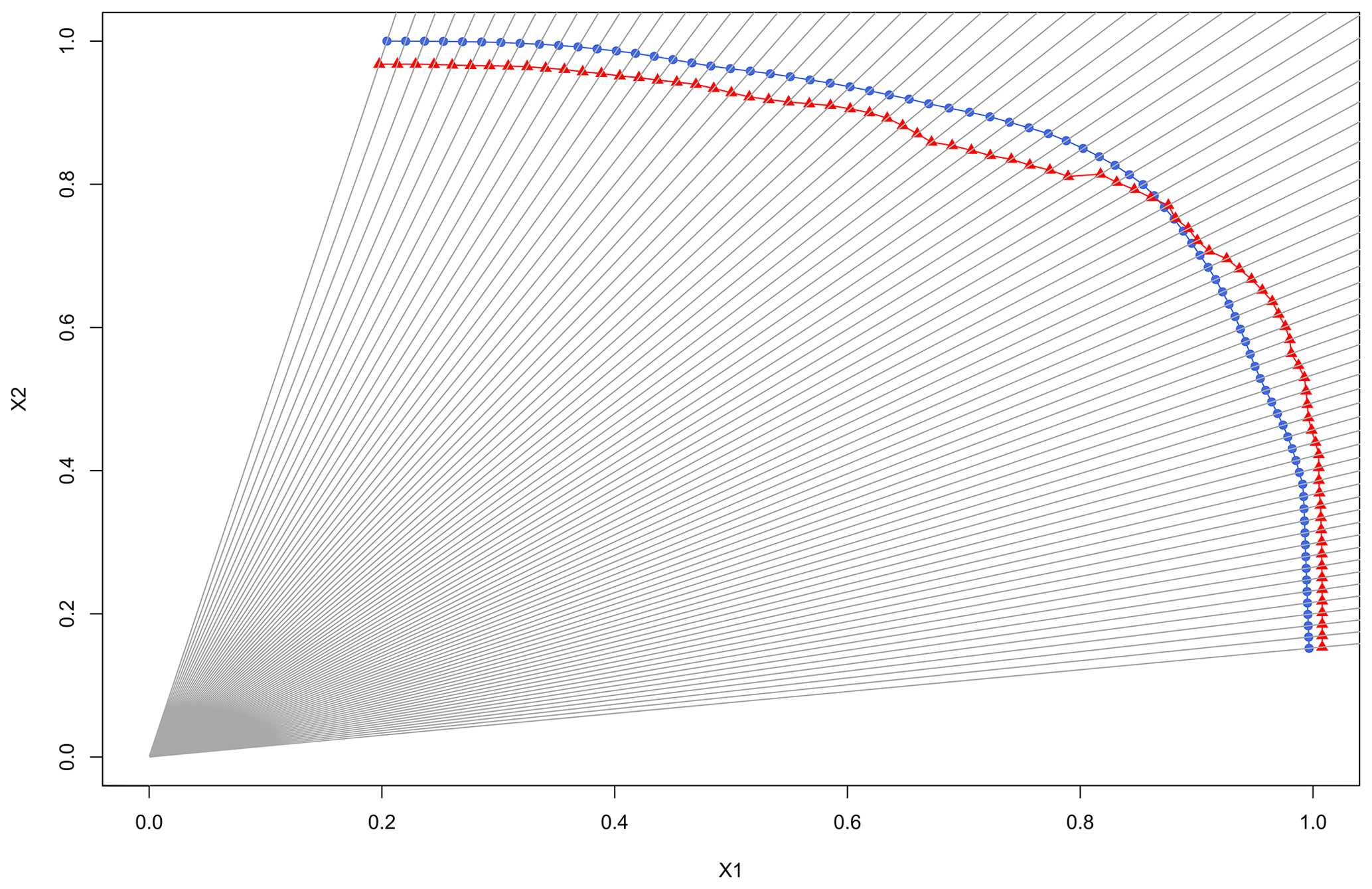
Figure 6Procedure for computation of the goodness-of-fit indicators. Two variables are given, X2 as a function of X1. The red triangles and red curve represent the modelled level curve from a given model. The blue circles and blue curve are the reference level curve from the underlying bivariate (X1, X2) distribution of the data. Distance between the curves is calculated along the radius at 80 (X1, X2) coordinates (e.g. between the blue circles and the red triangles).
We used a weighted Euclidean distance (wd) as a comparison criterion. The density of level curves (described in Sect. S2) allows one to weight the Euclidean distance of each of the 80 points by the local density of the curve. By weighting the Euclidean distance according to the reference bivariate distribution probability density function, we give more importance to the proper part of curve, where a bivariate event is more likely to occur, than to the naïve part (here the naïve part is defined as where the bivariate event is less likely to occur; Chebana and Ouarda, 2011; Volpi and Fiori, 2012).
3.3 Results
Two analyses are conducted in parallel, one for asymptotic dependence (AD) and one for asymptotic independence (AI). In the case of asymptotic dependence, the Gumbel copula is used with 5000 data points. The χ value is the one of interest under AD; values taken by χ have been presented in Sect. 3.1. For each χ value, we generated 100 realizations of the dataset from the same underlying bivariate distribution. The 100 realizations generated have two purposes: (i) increase the robustness of the results and (ii) create a confidence interval around the median which was set at the 95 % confidence level by taking the quantiles Q2.5 and Q97.5 of the 100 realizations. To confront this approach, we generated two sets of 100 realizations which showed very small variations in the values of Q2.5, Q50 and Q97.5 without impacting our interpretation of the results. In the case of asymptotic independence, the normal copula is used.
The marginal distributions do not have any impact on the dependence structure (Nelsen, 2006; Genest and Favre, 2007). We show in Appendix A that marginal distributions also have a very small impact on the estimation of dependence measures. All the methods used in this study include a transformation of marginal distributions and the fitting of a GPD above an extreme threshold (Sect. 2.3). By varying the marginal distribution of the variables of our synthetic dataset, we aim to capture uncertainties and errors arising from both the fitting of the marginal distributions and the dependence structure.
For both asymptotic dependence AD and asymptotic independence AI, the objective level curve lobj to be compared has been fixed at the probability pobj=0.001. For each of the 60 bivariate datasets, the six models presented are fitted to the 100 realizations. The dependence measures and as well as the level curve are estimated for each of the six models, with corresponding to each model. We then use the diagnostic tool and criteria presented in Sect. 3.2 to compare the performance of the models. From the 100 realizations, 100 level curves are generated for each model. Three curves are designed: (i) the 2.5 % quantile level curve, (ii) the median level curve and (iii) the 97.5 % quantile level curve.
In an analogous way, for each of the diagnostic tools presented in Sect. 3.2, three values are computed: (i) the 2.5 % quantile, (ii) the median and (iii) the 97.5 % quantile. To assess more accurately whether the models manage to represent the synthetic data in the large value extremes, we compared their fitting capabilities to a naïve approach. Here, the naïve approach is an empirical level curve. For each of the 60 synthetic datasets, we compute the wd of the empirical level curves to the reference curves following the same steps as for the six models. The empirical wd (wdnaïve) is therefore compared to the wd of each model. Models that represent the data with more accuracy than a naïve approach (wd<wdnaïve) are considered to be representative of the data. Figure 7 displays the values of the wd for each model applied to each bivariate dataset and highlight the cases where models outperform a naïve approach (bold blue). Squares are coloured according to the median of the wd, and thickness of the edges is proportional to the size the confidence interval (i.e. the distance between the quantiles Q2.5 and Q97.5).
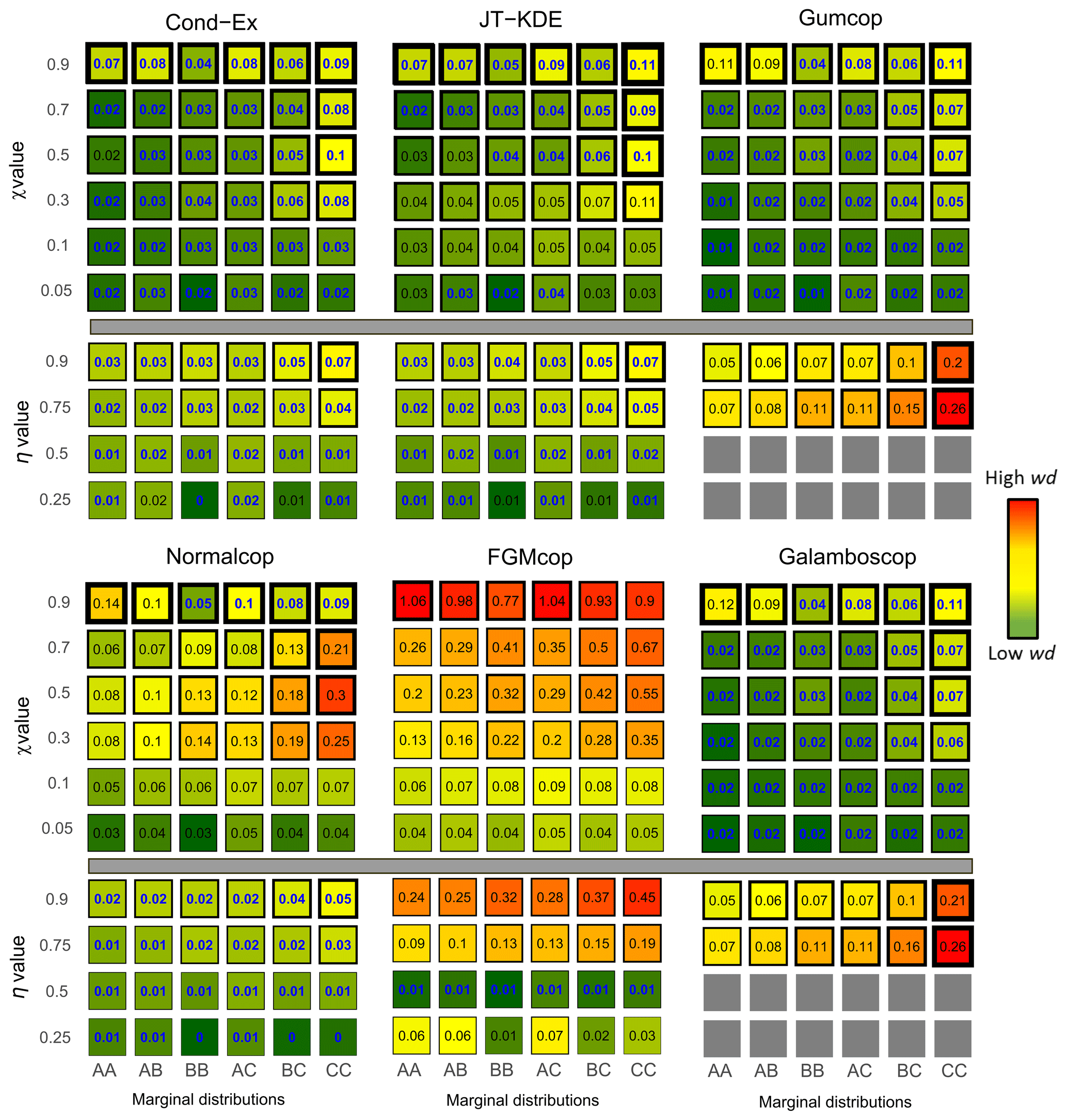
Figure 7Weighted normalized Euclidean distance (wd) to the reference curve for all 60 different synthetic datasets. Fitting capacities of each model are represented. Values in cells and colours represent the median wd from low (dark green) to high (red). Bold blue values highlight cases where models are representative of the data. Thickness of borders represent the 95 % uncertainty around the median value on a logarithmic scale.
It is important here to note that we tested more AD (36 %–60 %) than AI (24 %–40 %) cases. To assess the flexibility of models, additionally to comparison to the naïve approach, we also consider the proportion of cases where models have a wd<0.1. From Fig. 7, we observe the following:
-
The Gumbel and normal copulas, which have been used to generate the synthetic datasets with AD and AI, generally outperform all the other models in AD and AI cases respectively.
-
The conditional extremes model and the joint tail KDE model are the most flexible models tested here as they can handle (Cond-Ex) 98 % [72 %, 100 %] and (JT KDE) 97 % [65 %, 100 %] of the situation with a wd <0.1; these values reach 100 % for the AI cases. However, the Cond-Ex model is slightly more flexible, having a representative fit to more datasets (95 %) than the JT-KDE model (68 %).
-
The normal copula, even if asymptotically independent, is the most flexible copula model with wd < wdnaïve in 47 % of the cases, more than the number of AD datasets. The normal copula has a low wd (<0.1) in 76 % [60 %, 90 %] of the cases and has a representative fit to the data for every AI case and in some AD cases.
-
Gumbel and Galambos copulas have representative fits to only 57 % of the AD datasets. Among the 36 AD cases, they fail to represent only two with χ=0.9. It is important to note that both aforementioned copulas cannot handle complete independence (η=0.5) or negative dependence (η=0.25).
-
The FGM copula can only handle one type of extremal dependence, which is asymptotic independence (AI) with η=0.5. Consequently, it is the least flexible model in our results with a wd < wdnaïve in only 10 % of the cases.
-
Higher shape parameters of the margins are associated with poorer goodness of fit for all models. It is particularly striking with the conditional extremes approach which exhibits high uncertainty and high wd when both margins have a standard deviation σ=1.5.
The Cond-Ex and JT-KDE models provide close results according to Fig. 7 despite adopting very different approaches. Thus, their flexibility arises from their semi-parametric nature. Figure 7 also displays the uncertainty in the estimate of wd. For all models, a more accurate fit is accompanied with a reduction in uncertainties. However, both Cond-Ex and JT-KDE have on average more uncertainty around their wd despite their good fitting capabilities. On average, copulas tend to have less uncertainty due to their parametric nature.
However, the copulas are penalized by the weighting function as they usually reproduce quite well the naïve part of the curve. By considering again the percentage of situations with a criterion below 0.1, the normal copula has its performances reduced by the weighting function (−6 % compared to d). The JT-KDE model has its performance boosted by the weighting function (+7 % compared to d).
Results from the simulation study presented in the previous section (Sect. 3) can provide useful insights when modelling the interrelations between two natural hazards. In this section, we will show how results previously presented can be useful to identify the most relevant models for a given dataset according to its visual characteristics. The concordance (or discordance) of the relevant models can also increase (or decrease) confidence around the results.
The methodology for model selection presented here is composed of five steps to select the most relevant model estimate joint exceedance probability level curves:
- i.
The two-tail dependence measures are estimated empirically with a 95 % confidence interval. The dataset with a tail dependence measure falling into that confidence interval is suggested as analogue to the studied bivariate dataset. To select relevant combinations of marginal distribution, a scatterplot is compared visually to density plots for the 60 different datasets simulated in Sect. 3 and displayed in Fig. 5.
- ii.
From the aforementioned 60 datasets, a set of one to six analogous datasets (i.e. with similar bivariate distribution) is taken.
- iii.
A confidence score is used to compare the abilities of each model for the datasets selected in step (ii). For each model, the confidence score is the average of the computed weighted Euclidian distance wd for all datasets selected in step (ii). By taking the average of wd, a poor fit on one analogous dataset will have a high influence on the confidence score.
- iv.
Models are fit to the bivariate hazard dataset, and level curves from the most relevant models are kept.
- v.
Tail dependence measures are estimated using the most relevant model with a possible new iteration of the four previous steps according to the value of the dependence measures.
To produce a confidence interval as was carried out in the simulation study (Sect. 3) and to visually measure the uncertainty associated with each level curve as in Sect. 3, we use a non-parametric bootstrap procedure. The function tsboot from the R package “boot” (Davison and Hinkley, 1997; Canty and Ripley, 2019) is used to generate 100 bootstrapped replicate datasets with the same number of observations as the original (but some are repeated). Our six models are then fitted to the original dataset and on the 100 bootstrapped replicates.
4.1 Rain and wind gusts at Heathrow Airport (asymptotic independence)
Here, we study the interrelation between daily extreme wind gusts (w) and extreme rainfall (r) at London Heathrow Airport, UK, for the period 1 January 1971 to 31 May 2018, both introduced in Fig. 1. The relationship between wind and rainfall has been studied both globally (Martius et al., 2016) and locally (Johansson and Chen, 2003; Ming et al., 2015). These two hazards are often associated with different types of storms (Dowdy and Catto, 2017) and in particular with cyclones (Ming et al., 2015; Raveh-Rubin and Wernli, 2016). In southern England, these two hazards are mostly associated with extratropical cyclones in the winter season and thunderstorms in the summer season (Hawkes, 2008; Anderson and Klugmann, 2014; Webb and Elsom, 2016; Hendry et al., 2019).
The bivariate dataset used to study the interrelation between wind gusts and rainfall at Heathrow Airport is composed of the following data:
- a.
Daily wind gust (w). This is the daily maximum wind gust at the London Heathrow Airport (UK) weather station where a gust is the maximum value, over the observing cycle, of the 3 s running-average wind speed (WMO, 2019). Wind gusts are short-lived peaks in wind speed that can inflict great damage during a storm. However, this measurement might not capture the overall wind intensity (Met Office, 2019). The time range of the observations is 38 years, from 1 January 1971 to 31 May 2018, of which 74 d (0.4 % of the data) had no values recorded and all other values in the dataset had w>0 m s−1. These observation data have been provided by the Met Office (2019).
- b.
Daily rainfall (r). This is the daily total precipitation in a grid cell containing London Heathrow Airport (UK). The data have been extracted from the E-OBS gridded database (Cornes et al., 2018) which is formed from the interpolation of observations from 18 595 meteorological stations through Europe and the Mediterranean (including the Heathrow Airport station). It has been shown that E-OBS has excellent correlation with other high-resolution gridded datasets even if this correlation tends to decrease for extremes (Hofstra et al., 2009). However, by selecting a cell containing a weather station we limit uncertainties arising from interpolation. The spatial resolution in the E-OBS dataset is , and the period covered is 1950 to 2019. Data from 1 January 1971 to 31 May 2018 (38 years) in the cell containing Heathrow Airport are used, with a total of 6074 d (35.1 % of the dataset) having non-zero rainfall r>0 mm d−1.
From 1 January 1971 to 31 May 2018 there are a total of 17 318 d (including leap years). Our bivariate wind gust–rainfall dataset is composed of those values where there are both non-zero rainfall r>0 mm d−1 and wind gusts w>0 m s−1 recorded, resulting in a total of 6044 bivariate observations (34.9 % of the days in our record). An overview of both daily rainfall and daily wind gust is displayed in Fig. 8 in the form of monthly violin plots, where the probability density of w and r at different values are given, smoothed by a kernel density estimator.
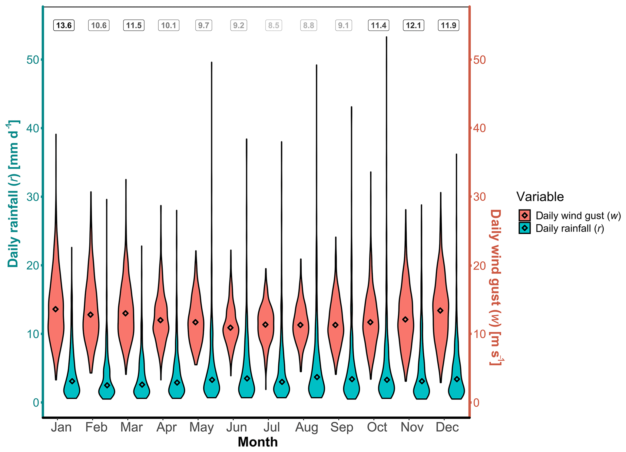
Figure 8Violin plots of daily wind gust w (red) and daily non-zero rainfall r (blue) by month for the period 1 January 1971 to 31 May 2018 at the Heathrow Airport weather station, UK. Diamonds represent the median of all values for that month from 1971–2018. Numbers at the top of the graph represent the average number of days per month where there is recorded both non-zero rainfall r>0 mm d−1 and wind gusts w>0 m s−1. Daily rainfall data from E-OBS (Cornes et al., 2018) and wind gust data (maximum 3 s wind velocity in a day) from the Met Office (2019).
From Fig. 8 we observe a seasonality in daily wind gust speed. January is the month with the highest median (diamond symbol) and range of most values in the violin plot, while July is the month with the lowest median and range of most values in the violin plot. The daily non-zero rainfall median per month varies between 2.5 mm in February and 3.5 mm in June, with the highest individual daily values occurring in October (53.3 mm d−1), May (49.6 mm d−1) and June (49.2 mm d−1). The dataset is also represented as a scatterplot in Fig. 9. The scatterplot will be used for the model selection methodology presented at the beginning of Sect. 4.
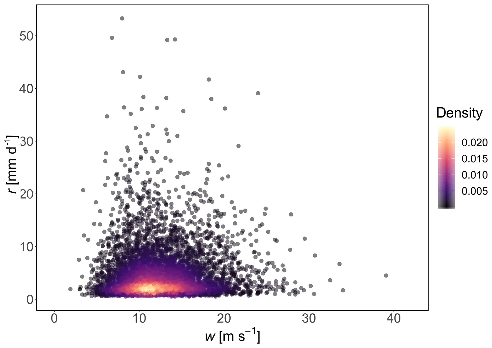
Figure 9Days where there are recorded both daily wind gust (m s−1) w and non-zero daily rainfall (mm d−1) r>0 mm d−1 at Heathrow Airport (London, UK) for the period 1971–2018. Daily rainfall data from E-OBS (Cornes et al., 2018) and wind gust data (the maximum 3 s wind velocity in a day) from the Met Office (2019). Colours (legend) represent the bivariate density estimated from a kernel density estimator with higher values and lighter colours representing a higher density of points at that bivariate value (r, w).
Extreme rainfall and extreme wind have a compound interrelation according to Tilloy et al. (2019). We then estimate the joint exceedance probability curve, corresponding to a PAND probability (Sect. 2.3).
We now go through the four steps presented for rainfall and wind gusts in Heathrow.
- i.
From Figs. 5 and 9, along with empirical estimates of χ and η, we hypothesize that over our time range 1971–2018, daily rainfall and daily maximum wind gusts in London Heathrow Airport are asymptotically independent or weakly dependent () and that both marginal distributions have a small shape parameter (AB, BB).
- ii.
This then gives us four analogous datasets, and it is then possible to visually infer from Fig. 6 which models are the most suitable for these conditions. The four analogous datasets are the following:
-
χ=0.05 and AB
-
χ=0.05 and BB
-
η=0.5 and AB
-
η=0.5 and BB
-
χ=0.1 and AB
-
χ=0.1 and BB.
-
- iii.
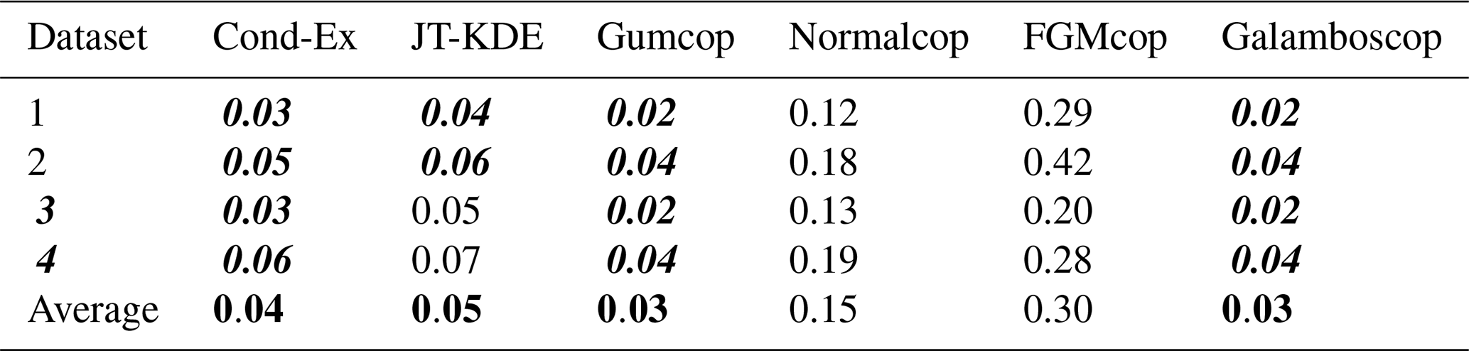
The confidence score for each model is the average of the weighted Euclidean distance wd from the four situations above. For the Gumbel and Galambos copulas, the cases of independence or negative dependence between variables are outside the modelling range (Sect. 2.3.1), and thus the confidence score for these models has been penalized by putting wd=1.0 for η=0.5 and η=0.25. The conditional extremes model has the smallest confidence score and is representative of all six analogous datasets. The JT-KDE model has a and is representative of four out of six analogous datasets. The FGM and normal copulas have a confidence score of and are only representative in AI cases. Gumbel and Galambos copulas have a confidence score of due to their penalty (Table 4).
Table 4Euclidian weighted distance (wd) for datasets 1 to 6 based on wind–rainfall and six models, along with confidence scores (average of the wd for datasets 1 to 6). In italic bold are highlighted the values below the naïve approach wd, and the average values of four models with confidence scores < 0.1 are highlighted in bold.
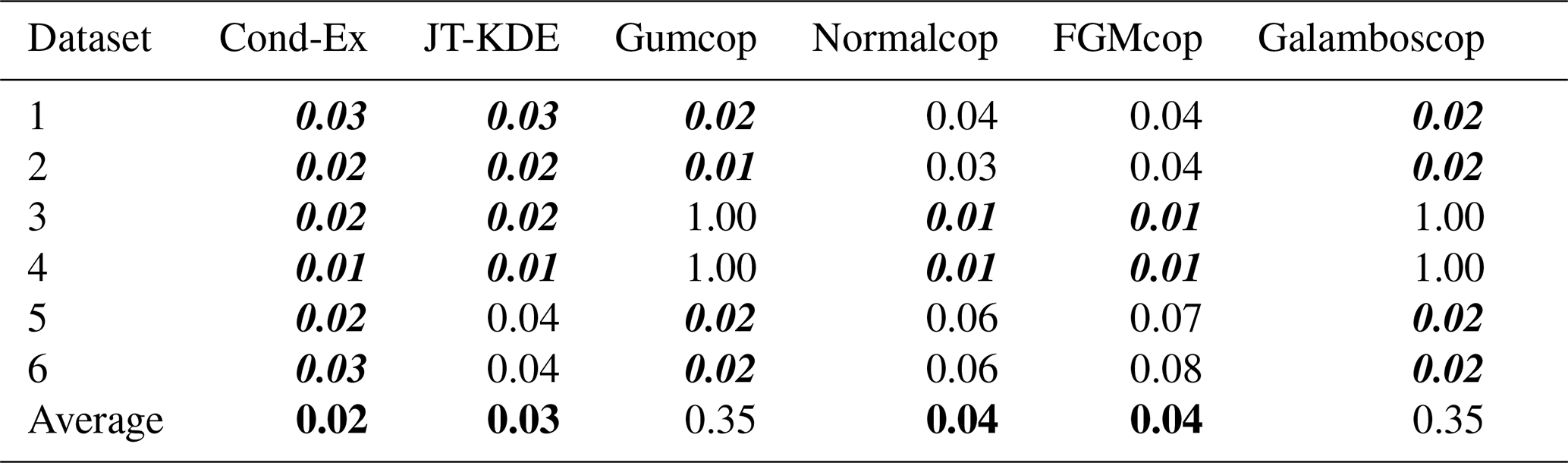
Table 5Estimates of dependence parameters χ and η for extreme rainfall and wind gust at Heathrow Airport for the time range 1971–2018.

According to these three first steps, the conditional extremes model appears to be the most suitable. However, we selected the four most relevant models for the bivariate dataset of daily rainfall and daily wind gust at London Heathrow Airport. The conditional extremes model, the JT-KDE model, the normal copula and the FGM copula all have low as can be seen in Table 4.
- iv.
For illustration and/or confronting our models with the data, the six models are fit to the dataset and joint exceedance level curves are produced with a joint exceedance probability set at p=0.001, corresponding to a bivariate return period of 8 years. However, another joint exceedance probability could have been chosen.
In Fig. 10 are displayed the level curves produced from the four models that were selected after steps (i) to (iii) above (Cond-Ex, JT-KDE, Normalcop and FGMcop), and their corresponding values are presented in bold numbers in Table 4.
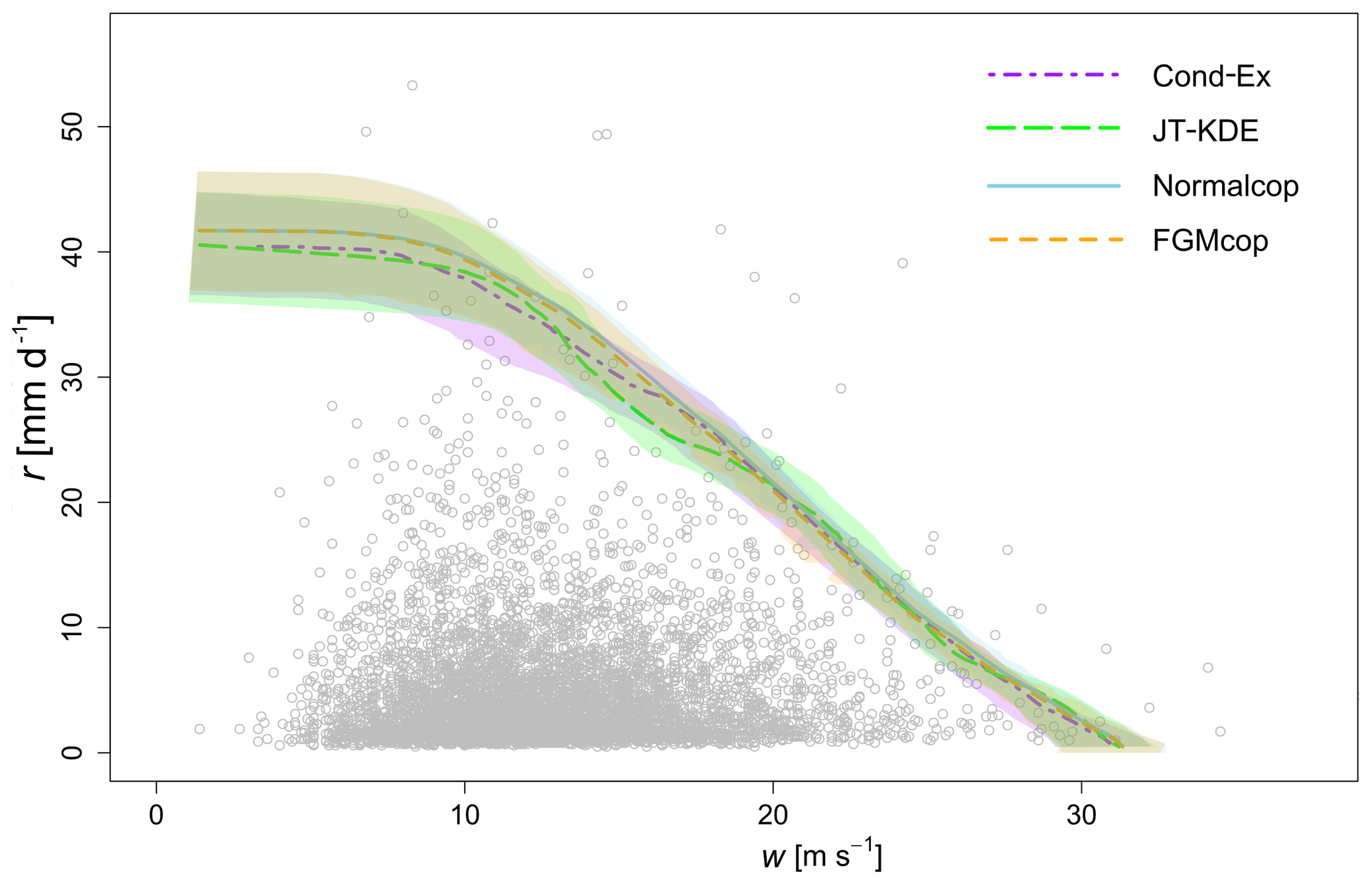
Figure 10Level curves for a PAND joint probability p=0.001 of daily wind gust and daily rainfall at Heathrow Airport (London, UK). Level curves from the four models selected through the model selection methodology are displayed.
From Fig. 10, we can observe that the conditional extremes model, the FGM copula and the normal copula all produce very similar joint exceedance curves and that their confidence intervals overlap. Table 5 displays the estimates (with bounds of the 95 % confidence interval) of the two dependence parameters χ and η from the six models. These estimates converge toward a very weak asymptotic dependence. However, the estimation of dependence parameters in near independence is highly uncertain (Sect. 3.3.2).
4.2 Daily wildfire number and temperature extremes in Portugal (asymptotic dependence)
Here we present a second example of applying our models to natural hazards data, using as a case study daily temperature and daily number of wildfires in Portugal. Wildfire variables such as daily number and burned area depend on many influences such as wind speed, direction and gustiness; topography; and type of fuel and soil moisture (Hincks et al., 2013). The aim of our study is not to decipher the processes leading to a wildfire but rather to provide an exemplar study examining the relationship between the two variables, daily temperature and daily number of wildfires, in a given case study area.
It has been shown that dry and warm conditions increase the risk of wildfire (Littell et al., 2009; AghaKouchak et al., 2018). Witte et al. (2011), establishing a direct link between a persistent heatwave and wildfire outbreaks in Russia and eastern Europe in 2010. The northern Mediterranean countries (Portugal, Spain, France, Italy and Greece) are particularly affected by summer fires (Vitolo et al., 2019).
Among these, Portugal holds the highest number of wildfires per land area (Pereira et al., 2011). There are many environmental and anthropogenic factors influencing the rural fire regime in Portugal and making its territory a fire-prone area. However, the majority of rural fires is recorded during hot and dry conditions in the summer (Pereira et al., 2011).
Here, we used the mainland Continental Portuguese Rural Fire Database, which includes 450 000 fires, covers the period 1980–2005 (Pereira et al., 2011) and includes data for all 18 districts in Portugal. This database is the largest such database in Europe in terms of total number of recorded fires in the 1980–2005 period (Pereira et al., 2011) and includes fires recorded down to a size of 0.001 ha. From the Continental Portuguese Rural Fire Database, we chose to focus on Porto District, which was the worst affected in the period (out of the 18 Portuguese districts) in terms of number of wildfires with 21.6 % of the total fire recorded in the dataset between 1980 and 2005. Porto District is situated in the northern part of Portugal (see Fig. 11), has an area of 2395 km2 and is one of the most populated districts of Portugal with an estimated population of 1 780 659 in 2019 (Instituto Nacional de Estatística Portugal, 2019).
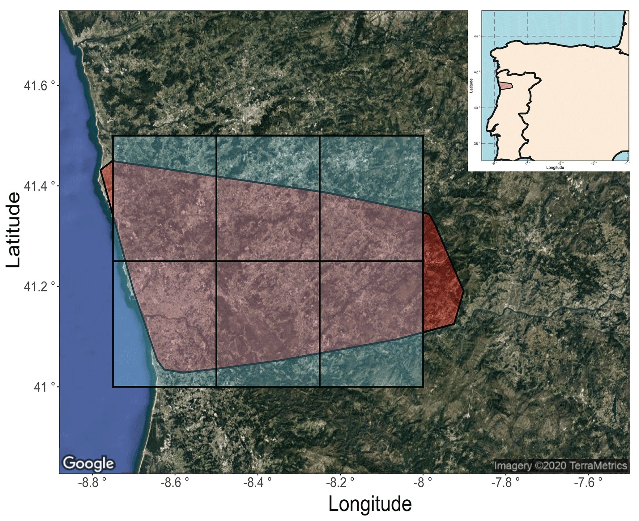
Figure 11Portugal study area for the interrelation between extreme hot temperature and wildfire-burned areas. The red area represents Porto District in Portugal, containing the studied wildfire-burned areas. The blue tiles represent cells from the high-resolution gridded dataset of daily climates over Europe (E-OBS; Cornes et al., 2018) containing mean daily temperature data. Satellite image retrieved with ggmap (Kahle and Wickham, 2013). © Google Maps (2020).
The bivariate dataset used to study the interrelation between extreme temperature and wildfire-burned areas in Porto District is composed of the following data:
- a.
Daily number of wildfires (f). The daily number of wildfires for the 26-year period 1980–2005 for Porto District was extracted from the Continental Portuguese Rural Fire Database dataset from Pereira et al. (2011). To account for undersampling of smaller wildfires in earlier years, and as suggested by Pereira et al. (2011), we used only those fires with a burned area AF≥0.1 ha, resulting in 59 522 fires, an average of 6.3 fires d−1 (for those days with at least one fire occurrence) over Porto District in Portugal (2395 km2).
- b.
Daily temperature data (t). Daily mean temperature was extracted from the E-OBS gridded dataset (Cornes et al., 2018). We approximate the area in red in Fig. 11 (Porto District) for each day with one temperature value by taking the average of daily temperatures in each of the six cells represented by blue rectangles in Fig. 11. This assumption reduces the confidence in return-level values and adds up with other interpolation uncertainties arising from the data (Hofstra et al., 2009). Moreover, the temperature in the six cells are strongly correlated (Pearson correlation coefficient ρ>0.98) and variations in temperature are mostly due to the distance to the sea and altitude (Miranda et al., 2002).
The 26 years from 1980 to 2005 have a total of 9496 d. Of these, a total of 3442 d (36 % of the days) have both non-zero days for number of wildfires and a mean temperature value, which are used in our final bivariate dataset. An overview of both daily mean temperature and daily number of wildfires is displayed in Fig. 12 in the form of monthly violin plots.

Figure 12Violin plot of those days with both daily mean temperature (red, upper violin plots) t and daily number of wildfires (blue, lower violin plots) f≥1 fire d−1, by month for the period 1980–2005 in Porto District (Portugal). Only those wildfires with burned area AF≥0.1 ha are included. Diamonds for both temperature and wildfires represent the median of all values in that month over the period of record. Numbers at the top of the graph represent the average number of days per month where there are recorded both a temperature value t and at least one wildfire (f≥1 fire d−1). Daily mean temperature data from E-OBS (Cornes et al., 2018) and wildfire data from Pereira et al. ( 2011).
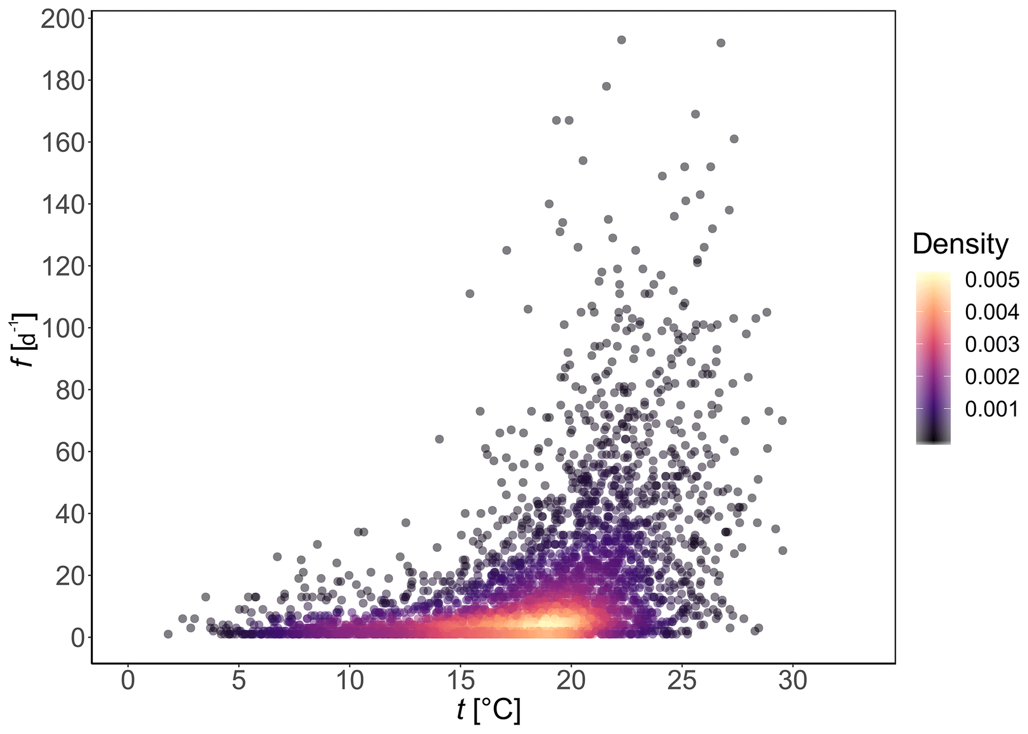
Figure 13Scatterplot of temperature dependence on wildfire occurrence in Porto District, Portugal, for the period 1980–2005, for those days where there are recorded both mean daily temperature (t) and at least one fire, with f the number of wildfires in 1 d. Only those wildfires with burned area AF≥0.1 ha are included. Daily mean temperature data from E-OBS (Cornes et al., 2018) and wildfire data from Pereira et al. (2011). Colours represent the bivariate density estimated from a kernel density estimator.
From Fig. 12 we observe the seasonality in daily mean temperature with January the coldest month (median =8.3 ∘C) and August the warmest (median =21.0 ∘C). Daily number of wildfires (with burned area AF≥0.1 ha) per month varies between median of 1.0–2.5 fire d−1 in winter months (November to February) and 7.0–22.5 fire d−1 in summer months (from June to September). The dataset is also represented as a scatterplot in Fig. 13. The scatterplot will be used for the model selection methodology presented at the beginning of Sect. 4.
As discussed in the beginning of this section, extreme (hot) temperature and wildfire are interrelated. Indeed, extreme (hot) temperature may promote the development of wildfires (Witte et al., 2011; Sutanto et al., 2020) According to Tilloy et al. (2019), this is a change condition interrelation (i.e. one hazard changes an environmental parameter that causes a move toward a change in the likelihood of another hazard). We then estimate the conditional exceedance probability curve (Sect. 2.3).
We now go through the four steps introduced at the beginning of Sect. 4.
- i.
From Figs. 5 and 13, along with empirical estimates of χ and η, we hypothesize that over our time range, there is asymptotic dependence for the mean daily temperature, the number of wildfires per day are asymptotically dependent (), and one marginal distribution has a slightly small shape parameter and the other one is heavily right-skewed (AC, BC).
- ii.
This then gives us four analogous datasets, and it is then possible to know from Fig. 8 which models are the most adapted to these conditions. The four datasets are the following:
-
χ=0.5 and AC
-
χ=0.5 and BC
-
χ=0.3 and AC
-
χ=0.3 and BC
-
- iii.
The confidence score for each model is the average of the wd from the four aforementioned datasets. Based on Table 6, the normal copula and FGM copula do not seem suitable for modelling the joint occurrence of wildfire and extreme temperature as these poorly fit the four datasets. The Gumbel and Galambos copulas () and the conditional extremes model () are representative of the four analogous datasets. The joint tail KDE model has a confidence score and is representative of two analogous datasets.
Table 6Weighted Euclidian distance (wd) for datasets 1 to 4 based on extreme temperature wildfire and six models, along with confidence scores (average of the wd for datasets 1 to 4). In italic bold are highlighted the values below the naïve approach wd, and the average values of the four models with confidence scores <0.1 are highlighted in bold.
According to these three first steps, we can identify the most relevant model for the bivariate dataset of daily maximum temperature and daily wildfire occurrence in Porto District: the Gumbel copula, Galambos copula, JT-KDE model and conditional extremes model are the most relevant models for our dataset.
- iv.
For illustration and/or the confronting of the models with the data, the six models are fit to the dataset and the joint exceedance level curves are produced with a joint exceedance probability set at p=0.001, corresponding to a bivariate return period of approximately 8 years.
In Fig. 14 are displayed the conditional level curves produced from the four models that were selected after steps (i) to (iii) and shown as bold values in Table 6 (Cond-Ex, JT-KDE, Gumcop and Galamboscop).
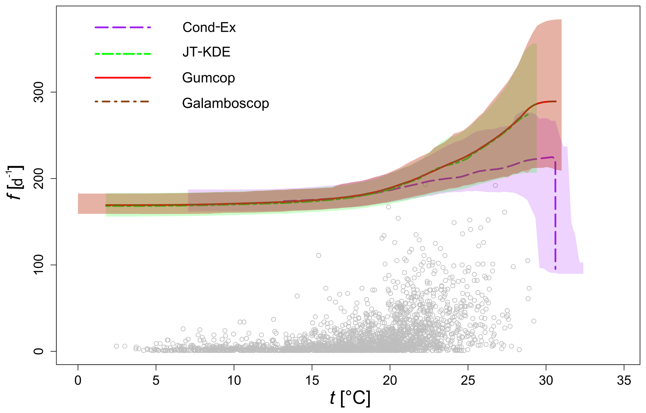
Figure 14Level curves for a PAND joint probability p=0.001 of daily mean temperature and daily number of wildfire occurrences in Porto District, Portugal, for the period 1980–2005. Level curves from the four models selected through the model selection methodology are displayed.
From Fig. 14, we can observe that JT-KDE and the Gumbel copula produce very similar conditional exceedance curves and that their confidence intervals strongly overlap. However, the conditional extremes model provides a lower estimate than the other approaches, the number of wildfires being conditional on the temperature being above a given threshold.
In Table 7, we present the estimates (with bounds of the 95 % confidence interval) of the two dependence parameters χ and η from the six models, providing a bit more insight into the dependence structure. These estimates converge toward a moderate asymptotic dependence varying from χ=0.15 (Cond-Ex) to χ=0.47 (Gumcop). Even if all models tend to show asymptotic dependence between the two variables, estimates of η are less than 1.0 for the normal copula, the JT-KDE model and the Cond-Ex with values varying between 0.67 and 0.79. This still implies a positive association between the two variables.
Table 7Estimates of dependence parameters χ and η for mean daily temperature and daily occurrences of wildfire in Porto District for the period 1980–2005.

Quantifying and measuring the interrelations between different natural hazards is a key element when adopting a multi-hazard approach (Gill and Malamud, 2014; Leonard et al., 2014). In this study, we focused on statistical approaches that are often used to characterize and model interrelations between hazards. Another focus has been on modelling relationships between hazards at an extreme level. In total six statistical models with different characteristics (nature of asymptotic dependence, parametric and semi-parametric) were compared. Some of these models have already been used to study compound extremes in hydrology and climatology (Hao et al., 2018; Liu et al., 2018; Sadegh et al., 2018; Cooley et al., 2019). However, these have not been compared over a broad range of bivariate datasets and applied to the same natural hazards in the same location.
This section will discuss the following three themes before a short conclusion: (a) choices influencing the results of the simulation study, (b) uncertainties at the interface between asymptotic dependence and asymptotic independence, and (c) possible extensions of this approach to more than two hazards.
Choices influencing the results of the simulation study. This study aimed to assess the fitting ability of several bivariate models to a broad range of datasets. In order to do so, models were compared in their ability to reproduce an extreme level curve (see Sect. 3.2.1). The level curve corresponding to the PAND probability has been selected as a comparison point because it is commonly used in the literature and is relevant for practitioners. The choice of this level curve and its shape could influence our results. The extreme level curve probability was set at p=0.001. The multivariate regular variation framework (Resnick, 1987) provides evidence supporting the fact that the dependence structure remains identical in the whole extreme domain. However, some results shown in Sect. 3.3 might have been influenced by the value of the joint exceedance probability. In particular, it is likely that when decreasing the level curve probability (i.e. to more extreme values), the flexibility and abilities of the asymptotically independent normal copula will decrease.
There are many copulas other than the four selected in this study (Nelsen, 2006; Sadegh et al., 2017) that have been developed. Nevertheless, we believe the four copulas used in this study are suitable for bivariate extreme value analysis and are amongst the most widely used in the literature (Genest and Favre, 2007; Genest and Nešlehová, 2013). Another influential choice in this study has been the number of synthetic data points generated in each realization of the dataset.
The number of data points and dataset size is an important influence on uncertainty in natural hazard modelling and probabilistic approaches (Frau et al., 2017; Liu et al., 2018). For each simulation, we simulated n=5000 data points. Some other simulation studies took a higher number of data points (Zheng et al., 2014; Cooley et al., 2019); however, we replicated the simulation 100 times and produced confidence intervals, thus ensuring consistency of our results. We also found that threshold selections, to fit the generalized Pareto distributions of the marginal distributions and to estimate the extremal dependence measures, have an influence on our results.
Uncertainties at the interface between asymptotic dependence and asymptotic independence. From the results of the simulation study (Sect. 3.3) and the two case study applications (Sect. 4), one can observe that the interface between asymptotic dependence and asymptotic independence can be unclear. In Sect. 3.3, we discussed the decrease in model performance and the increase in uncertainty for low values of χ and high values of η. Taking the assumption of asymptotic independence or asymptotic dependence can have a significant impact on the estimation of joint return levels. We find that extra care is required when dealing with bivariate datasets which are near independence as in Sect. 4.1.
Possible extension of the approaches to more than two hazards. As presented through this paper, the study of interrelations between natural hazards has primarily been carried out by hazard pairs (e.g. Gill and Malamud, 2014). Dependence measures and a variety of different models or level curves, all presented in this article, are powerful tools to assess, quantify and model interrelations between two hazards. However, in many cases, multi-hazard events include more than two hazards interacting in various ways (e.g. Gill and Malamud, 2014; Leonard et al., 2014). The use of models presented in this article can be extended to more than two variables, sometimes with disadvantages. One of these disadvantages is that the parametric nature of copulas leads to a lack of flexibility when going to higher dimensionality (Bevacqua et al., 2017; Hao et al., 2018). The JT-KDE and Cond-Ex models are suitable for higher dimensions (Davison and Huser, 2015; Cooley et al., 2019), although these have not been tested for high dimensional multi-hazard modelling yet (Tilloy et al., 2019).
Recent research conducted suggest pair-copula construction (Bedford and Cooke, 2002; Hashemi et al., 2016; Bevacqua et al., 2017, Liu et al., 2018) and non-parametric Bayesian networks (NPBNs; Hanea et al., 2015; Couasnon et al., 2018) can be used to model multi-hazard events with more than two hazards. The vine copula framework allows one to select different bivariate copulas for each pair of variables, providing a great flexibility in dependence modelling (Brechmann and Schepsmeier, 2013; Hao and Singh, 2016). Non-parametric Bayesian networks, which are associated with the structure of Bayesian networks and copulas (Hanea, 2010; Hanea et al., 2010, 2015), have been used to study multiple dependences between river discharge and storm surges in the USA during a hurricane (Couasnon et al., 2018).
In conclusion, we have compared and examined the strengths and weaknesses of six distinct bivariate extreme models in the context of hazard interrelations. These six models are grounded in multivariate extreme value theory and represent the diversity of approaches (e.g. non-parametric vs. parametric) currently applied to hazard interrelation analysis. With this study we aimed to contribute to a better understanding of the applicability of bivariate extreme models to a wide range of natural hazard interrelations. The methodology developed in this article is aimed to be widely applicable to a variety of different hazards and different interrelations, here represented by the 60 synthetic datasets created.
Abilities of each model have been assessed with two metrics: (i) dependence measure; (ii) bivariate return level (level curves). These two metrics and the different diagnostic tools developed in this study offer new intuitive ways to decipher the dependence between two variables. We recommend selecting a range of models rather than one when studying interrelations between two hazards. To highlight the benefits of the systematic framework developed, we studied the dependence between extremes (natural hazards) of the following environmental data: (i) daily precipitation accumulation and daily maximum wind gust (maximum over a period of 3 s) at Heathrow Airport (UK) over the period 1971–2018 and (ii) daily mean temperature and daily number of wildfires in Porto District, Portugal, over the period 1980–2005. The two datasets represent different hazard interrelations: (i) compound interrelation between extreme wind and extreme rainfall and (ii) change condition interrelation where higher air temperatures change conditions for wildfire occurrence. In both cases, a sample of the most relevant model among the six used in this study has been selected and fitted to the bivariate datasets. The good agreement in the estimation of the bivariate return period between models corroborates the relevance of the comparison metrics we developed.
A1 Tail dependence measure estimations
Tail dependence measures η and χ are estimated by each model. For copulas, these measures are related to the copula parameters. In our set of four copulas, two are asymptotically dependent (Gumbel and Galambos) with η=1 and two are asymptotically independent (normal and FGM) with χ=0.
For the non-parametric joint tail approach, the χ and η measures are estimated following the procedure used by Winter (2016). For the conditional model, both measures are estimated from the simulated points. Marginal distributions (X1, X2) are transformed to the uniform margins (U1, U2). The χ measure is estimated by calculating the probability (Eq. 4). The η measure is estimated in two steps. First we estimate as (Coles et al., 1999)
for , with u being a sufficiently high threshold. Second, the η measure is estimated from (Eq. A1).
To compare the estimated dependence measure to the reference value, the root-mean-square error (RMSE), a measure of efficiency that accounts for both the bias and variance in the estimates, is used, similarly to Zheng et al. (2014). Similarly to the metrics used in Sect. 3, the RMSE is calculated from 100 realizations of the 60 datasets.
A2 Comparison of model abilities
The estimation of the dependence measure is an important step in bivariate analysis (Coles et al., 1999; Heffernan, 2000; Zheng et al., 2013, 2014; Dutfoy et al., 2014). Models have also been compared on their ability to estimate the dependence measures χ and η. Results arising from this comparison provide a different perspective on the abilities of each model. Figure A1 shows the RMSE of the dependence measure estimations for each of the 60 synthetic datasets.
From Fig. A1, we observe the following:
-
Marginal distributions do not have a significant impact on the accuracy of the estimation of these measures for the copulas.
-
Marginal distributions have a small impact on the estimation of the dependence measures for the conditional extremes model and the joint tail model; however this impact is not as important as for the level curve estimation.
-
All copulas estimate very accurately the dependence measure within their operating range (AI for normal copula, near independence for FGM copula and AD for Gumbel and Galambos copulas). However, only the conditional extremes model and the joint tail model can estimate both η and χ.
-
The dependence measure estimator used in the joint tail KDE approach offers slightly more accurate estimation, particularly for η.
-
Estimation performance of both joint tail KDE and condition extreme models decreases when approaching the interface between asymptotic dependence and asymptotic independence. The RMSE at χ=0.05 is close to 100 % of the value of χ while the RMSE at η=0.9 is at its highest for both the Cond-Ex and JT-KDE models. It is then hard to decipher with confidence the nature of the dependence in the asymptotic domain for low χ values and high η values.
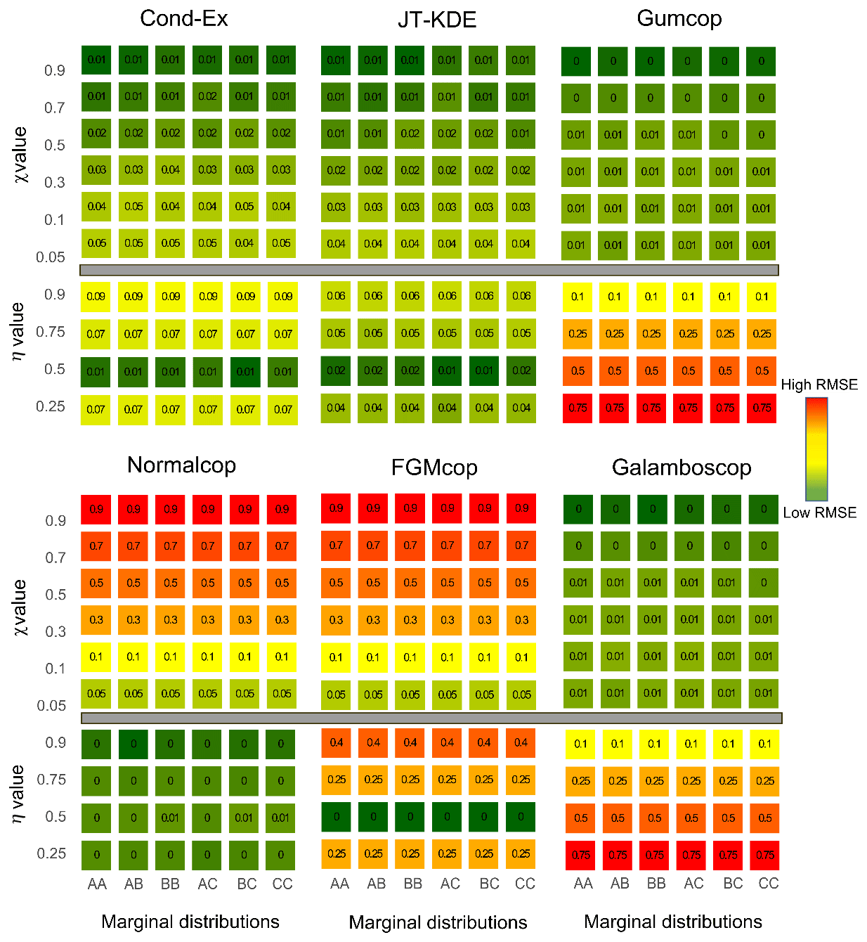
Figure A1RMSE (root-mean-square error) in the estimated dependence measures compared to the reference for all 60 different datasets. Fitting capacities of each model are represented. Values in cells and colours represent the median RMSE from low (dark green) to high (red). Thickness of cell borders represent the 95 % uncertainty around the median value.
The codes used to produce synthetic data and the six models used in this study are publicly available on GitLab: https://gitlab.com/doudeg/bivariate_models.git (Tilloy, 2020a).
We acknowledge the E-OBS dataset from the EU FP6 project UERRA (http://www.uerra.eu, UERRA, 2020) and the data providers in the ECA&D project (https://www.ecad.eu, ECA&D, 2020). The wind gust data were obtained from the UK Met Office. The fire data are available from Pereira et al. (2011). The bivariate (wildfire, temperature) data used are available at https://doi.org/10.5281/zenodo.3686962 (Tilloy, 2020b).
The supplement related to this article is available online at: https://doi.org/10.5194/nhess-20-2091-2020-supplement.
All authors discussed the whole plan of this article. AT designed and implemented all the experiments, prepared all the data, and finished the draft, including all figures in the article. BDM, HW and AJL revised the article. HW supported the methods and techniques.
Bruce D. Malamud is on the editorial board of this journal (the article has been overseen independently by another editor of this journal).
This article is part of the special issue “Advances in extreme value analysis and application to natural hazards”. It is not associated with a conference.
The first author was supported by an EDF R&D PhD studentship.
Aloïs Tilloy was supported by an EDF Energy R&D PhD studentship.
This paper was edited by Thomas Wahl and reviewed by two anonymous referees.
AghaKouchak, A., Huning, L. S., Chiang, F., Sadegh, M., Vahedifard, F., Mazdiyasni, O., Moftakhari, H., and Mallakpour, I.: How do natural hazards cascade to cause disasters?, Nature, 561, 458–460, 2018.
Aitchison, J.: Lognormal Distribution, Cambridge University Press., Cambridge, UK, 1957.
Akaike, H.: A new look at the statistical model identification, IEEE Trans. Automat. Contr., 19, 716–723, 1974.
Anderson, G. and Klugmann, D.: A European lightning density analysis using 5 years of ATDnet data, Nat. Hazards Earth Syst. Sci., 14, 815–829, https://doi.org/10.5194/nhess-14-815-2014, 2014.
Arnold, T. B. and Emerson, J. W.: Nonparametric goodness-of-fit tests for discrete null distributions, R J., 3, 34–39, 2011.
Barriopedro, D., Fischer, E. M., Luterbacher, J., Trigo, R. M., and García-Herrera, R.: The hot summer of 2010: Redrawing the temperature map of Europe, Science, 332, 220–224, 2011.
Bedford, T. and Cooke, R. M.: Vines : A New Graphical Model for Dependent Random Variables, Ann. Stat., 30, 1031–1068, 2002.
Bevacqua, E., Maraun, D., Hobæk Haff, I., Widmann, M., and Vrac, M.: Multivariate statistical modelling of compound events via pair-copula constructions: analysis of floods in Ravenna (Italy), Hydrol. Earth Syst. Sci., 21, 2701–2723, https://doi.org/10.5194/hess-21-2701-2017, 2017.
Brechmann, E. C. and Schepsmeier, U.: Modeling Dependence with C- and D-Vine Copulas: The RPackage CDVine, J. Stat. Softw., 52, 1–27, 2013. https://doi.org/10.18637/jss.v052.i03, 2013.
Canty, A. and Ripley, B. D.: boot: Bootstrap R (S-Plus) Functions, available at: https://cran.r-project.org/web/packages/boot/citation.html (last access: 22 June 2020), 2019.
CCR (Caisse Centrale de Réassurance): E-risk database, Paris, France, available at: https://catastrophes-naturelles.ccr.fr (last access: 1 December 2019), 2019.
Chebana, F. and Ouarda, T. B. M. J.: Multivariate quantiles in hydrological frequency analysis, Environmetrics, 22, 63–78, 2011.
Clare, M. A., Talling, P. J., Challenor, P. G., and Hunt, J. E.: Tempo and Triggering of Large Submarine Landslides: Statistical Analysis for Hazard Assessment, in: Advances in Natural and Technological Hazards Research, Vol. 41, edited by: Lamarche, G., Mountjoy, J., Bull, S., Hubble, T., Krastel, S., Lane, E., Micallef, A., Moscardelli, L., Mueller, C., Pecher, I., and Woelz, S., Springer International Publishing, Cham, Switzerland, 509–517, 2016.
Coles, S.: An Introduction to Statistical Modelling of Extreme Values, Springer London, London, UK, 2001.
Coles, S. and Tawn, J. A.: Modelling extreme multivariate events, J. R. Stat. Soc., 53, 285–339, 1991.
Coles, S., Heffernan, J. E., and Tawn, J. A.: Dependence measure for extreme value analyses, Extremes, 1225, 41–42, 1999.
Cooley, D., Thibaud, E., Castillo, F., and Wehner, M. F.: A nonparametric method for producing isolines of bivariate exceedance probabilities, Extremes, 22, 373–390, 2019.
Cornes, R. C., van der Schrier, G., van den Besselaar, E. J. M., and Jones, P. D.: An ensemble version of the E-OBS temperature and precipitation data sets, J. Geophys. Res.-Atmos., 123, 9391–9409, 2018.
Couasnon, A., Sebastian, A., and Morales-Nápoles, O.: A copula-based Bayesian network for modeling compound flood hazard from riverine and coastal interactions at the catchment scale: an application to the Houston ship channel, Texas, Water, 10, 1190, https://doi.org/10.3390/w10091190, 2018.
Davison, A. C. and Hinkley, D. V.: Bootstrap Methods and Their Applications, Cambridge University Press, Cambridge, UK, 1997.
Davison, A. C. and Huser, R.: Statistics of extremes, Annu. Rev. Stat. Appl., 2, 203–235, 2015.
De Haan, L. and De Ronde, J.: Sea and wind: multivariate extremes at work, Extremes, 1, 7–45, 1998.
De Michele, C., Salvadori, G., Passoni, G., and Vezzoli, R.: A multivariate model of sea storms using copulas, Coast. Eng., 54, 734–751, 2007.
De Haan, L. and Resnick, S. I.: Limit theory for multivariate sample extremes, Z. Wahrscheinlichkeit., 40, 317–337, 1977.
Dowdy, A. J. and Catto, J. L.: Extreme weather caused by concurrent cyclone, front and thunderstorm occurrences, Sci. Rep., 7, 1–8, 2017.
Duong, T.: ks: Kernel density estimation and kernel discriminant analysis for multivariate data, R, J. Stat. Softw., 21, 1–16, https://doi.org/10.18637/jss.v021.i07, 2007.
Duong, T.: Non-parametric smoothed estimation of multivariate cumulative distribution and survival functions, and receiver operating characteristic curves, J. Korean Stat. Soc., 45, 33–50, 2015.
Dutfoy, A., Parey, S., and Roche, N.: Multivariate extreme value theory - A tutorial with applications to hydrology and meteorology, Depend. Model., 2, 30–48, 2014.
ECA&D: ECA&D Project, available at: https://www.ecad.eu/, last access: 12 February 2020.
Frau, R., Andreewsky, M., and Bernardara, P.: The use of historical information for regional frequency analysis of extreme skew surge, Nat. Hazards Earth Syst. Sci., 18, 949–962, https://doi.org/10.5194/nhess-18-949-2018, 2018.
Genest, C. and Favre, A.-C.: Everything you always wanted to know about copula modeling but were afraid to ask, J. Hydrol. Eng., 12, 347–368, 2007.
Genest, C. and Nešlehová, J.: Copula Modeling for Extremes, in: Encyclopedia of Environmetrics, John Wiley & Sons Ltd, Chichester, UK, 1–6, 2013.
Genest, C., Rémillard, B., and Beaudoin, D.: Goodness-of-fit tests for copulas: A review and a power study, Insur. Math. Econ., 44, 199–213, 2009.
Genest, C., Kojadinovic, I., Nešlehová, J., and Yan, J.: A goodness-of-fit test for bivariate extreme-value copulas, Bernoulli, 17, 253–275, 2011.
Gill, J. C. and Malamud, B. D.: Reviewing and visualizing the interactions of natural hazards, Rev. Geophys., 52, 680–722, 2014.
Gouldby, B., Wyncoll, D., Panzeri, M., Franklin, M., Hunt, T., Hames, D., Tozer, N., Hawkes, P., Dornbusch, U., and Pullen, T.: Multivariate extreme value modelling of sea conditions around the coast of England, Proc. Inst. Civ. Eng. Marit. Eng., 170, 3–20, 2017.
Hanea, A., Kurowicka, D., Cooke, R. M. and Ababei, D. A.: Mining and visualising ordinal data with non-parametric continuous BBNs, Comput. Stat. Data Anal., 54, 668–687, 2010.
Hanea, A., Morales Napoles, O., and Ababei, D.: Non-parametric Bayesian networks: Improving theory and reviewing applications, Reliab. Eng. Syst. Saf., 144, 265–284, 2015.
Hao, Z. and Singh, V. P.: Review of dependence modeling in hydrology and water resources, Prog. Phys. Geogr., 40, 549–578, 2016.
Hao, Z., Hao, F., Singh, V. P., and Ouyang, W.: Quantitative risk assessment of the effects of drought on extreme temperature in eastern China, J. Geophys. Res.-Atmos., 122, 9050–9059, 2017.
Hao, Z., Singh, V., and Hao, F.: Compound extremes in hydroclimatology: A review, Water, 10, 718, https://doi.org/10.3390/w10060718, 2018.
Hashemi, S. J., Khan, F. I. and Ahmed, S.: Multivariate probabilistic safety analysis of process facilities using the Copula Bayesian Network model, Comput. Chem. Eng., 93, 128–142, 2016.
Hatvani-Kovacs, G., Belusko, M., Pockett, J., and Boland, J.: Assessment of heatwave impacts, Procedia. Engineer., 169, 316–323, 2016.
Hauser, M., Orth, R., and Seneviratne, S. I.: Role of soil moisture vs. recent climate change for heat waves in western Russia, Geophys. Res. Lett., 43, 2819–2826, 2015.
Hawkes, P. J.: Joint probability analysis for estimation of extremes, J. Hydraul. Res., 46, 246–256, 2008.
Hawkes, P. J., Gouldby, B. P., Tawn, J. A., and Owen, M. W.: The joint probability of waves and water levels in coastal engineering design, J. Hydraul. Res., 40, 241–251, 2002.
Heffernan, J. E.: A directory of coefficients of tail dependence, Extremes, 3, 279–290, 2000.
Heffernan, J. E. and Tawn, J. A.: A conditional approach for multivariate extreme values (with discussion), J. Roy. Stat. Soc. B, 66, 497–546, 2004.
Hendry, A., Haigh, I. D., Nicholls, R. J., Winter, H., Neal, R., Wahl, T., Joly-Laugel, A., and Darby, S. E.: Assessing the characteristics and drivers of compound flooding events around the UK coast, Hydrol. Earth Syst. Sci., 23, 3117–3139, https://doi.org/10.5194/hess-23-3117-2019, 2019.
Hilal, S., Poon, S. H., and Tawn, J.: Hedging the black swan: Conditional heteroskedasticity and tail dependence in S&P500 and VIX, J. Bank. Financ., 35, 2374–2387, 2011.
Hincks, T. K., Malamud, B. D., Sparks, R. S. J., Wooster, M. J., and Lynham, T. J.: Risk assessment and management of wildfires, in: Risk and uncertainty assessment for natural hazards, edited by: Rougier, J., Sparks, S., and Hill, L., Cambridge University Press, Cambridge, 398–444, 2013.
Hofstra, N., Haylock, M., New, M., and Jones, P. D.: Testing E-OBS European high-resolution gridded data set of daily precipitation and surface temperature, J. Geophys. Res.-Atmos., 114, D21101, https://doi.org/10.1029/2009JD011799, 2009.
Huser, R.: Statistical Modeling and Inference for Spatio-Temporal Extremes, PhD thesis, EPFL, available at: https://infoscience.epfl.ch/record/188557?ln=en (last access: 28 January 2020), 2013.
Instituto National de Estatistica Portugal, https://www.ine.pt/xportal/xmain?xpid=INE&xpgid=ine_indicadores&indOcorrCod=0004168&contexto=bd&selTab=tab2, last access: 1 December 2019.
Joe, H.: Multivariate models and multivariate dependence concepts, Chapman and Hall/CRC, London, 1997.
Johansson, B. and Chen, D.: The influence of wind and topography on precipitation distribution in Sweden: Statistical analysis and modelling, Int. J. Climatol., 23, 1523–1535, 2003.
Kahle, D. and Wickham, H.: ggmap: Spatial Visualization with ggplot2, R J., 5, 144–161, 2013.
Keef, C., Papastathopoulos, I., and Tawn, J. A.: Estimation of the conditional distribution of a multivariate variable given that one of its components is large: Additional constraints for the Heffernan and Tawn model, J. Multivar. Anal., 115, 396–404, 2013.
Koopmans, L. H., Owen, D. B., and Rosenblatt, J. I.: Confidence intervals for the coefficient of variation for the normal and log normal distributions, Biometrika, 51, 25–32, 1964.
Ledford, A. W. and Tawn, J. A: Statistics for near independence in multivariate extreme values, Biometrika, 83, 169–187, 1996.
Ledford, A. W. and Tawn, J. A.: Modelling dependence within joint tail regions, J. Roy. Stat. Soc. B, 59, 475–499, 1997.
Ledford, A. W. and Tawn, J. A.: Diagnostics for dependence within time series extremes, J. Roy. Stat. Soc. B, 65, 521–543, 2003.
Leonard, M., Westra, S., Phatak, A., Lambert, M., van den Hurk, B., McInnes, K., Risbey, J., Schuster, S., Jakob, D., and Stafford-Smith, M.: A compound event framework for understanding extreme impacts, Wiley Interdiscip. Rev. Clim. Chang., 5, 113–128, 2014.
Littell, J. S., McKenzie, D., Peterson, D. L., and Westerling, A. L.: Climate and wildfire area burned in western US ecoprovinces, 1916–2003, Ecol. Appl., 19, 1003–1021, 2009.
Liu, Z., Cheng, L., Hao, Z., Li, J., Thorstensen, A., and Gao, H.: A framework for exploring joint effects of conditional factors on compound floods, Water Resour. Res., 54, 2681–2696, 2018.
Loukatou, A., Howell, S., Johnson, P., and Duck, P.: Stochastic wind speed modelling for estimation of expected wind power output, Appl. Energ., 228, 1328–1340, 2018.
Malamud, B. D. and Turcotte, D. L.: Self-affine time series: I. Generation and analyses, Adv. Geophys., 40, 1–90, 1999.
Malamud, B. D. and Turcotte, D. L.: The applicability of power-law frequency statistics to floods, J. Hydrol., 322, 168–180, 2006.
Martius, O., Pfahl, S., and Chevalier, C.: A global quantification of compound precipitation and wind extremes, Geophys. Res. Lett., 43, 7709–7717, 2016.
Maulik, K. and Resnick, S.: Characterizations and examples of hidden regular variation, Extremes, 7, 31–67, 2005.
Mazas, F. and Hamm, L.: An event-based approach for extreme joint probabilities of waves and sea levels, Coast. Eng., 122, 44–59, 2017.
Met Office: How we measure wind: available at: https://www.metoffice.gov.uk/weather/guides/observations/how-we-measure-wind, last access: 12 November 2019.
Ming, X., Xu, W., Li, Y., Du, J., Liu, B., and Shi, P.: Quantitative multi-hazard risk assessment with vulnerability surface and hazard joint return period, Stoch. Environ. Res. Risk Assess., 29, 35–44, 2015.
Miranda, P. M. A., Coelho, F. E. S., Tomé, A. R., Valente, M. A., Carvalho, A., Pires, C., Pires, H. O., Pires, V. C., and Ramalho, C.: 20th Century Portuguese Climate and Climate Scenarios, in: Climate Change in Portugal. Scenarios, Impacts and Adaptation Measures – SIAM Project, edited by: Santos, F. D., Forbes, K., and Moita, R., Gradiva Publishers, Lisbon, 28–83, 2002.
Nelsen, R.: An Introduction to Copulas, Springer New York, New York, NY, USA, 2006.
Nguyen Sinh, H., Lombardo, F. T., and Letchford, C.: Multivariate simulation for assessing the joint wind and ice hazard in the United States, J. Wind Eng. Ind. Aerodyn., 184, 436–444, 2019.
Pereira, M. G., Malamud, B. D., Trigo, R. M., and Alves, P. I.: The history and characteristics of the 1980–2005 Portuguese rural fire database, Nat. Hazards Earth Syst. Sci., 11, 3343–3358, https://doi.org/10.5194/nhess-11-3343-2011, 2011.
Perkins, S. E.: A review on the scientific understanding of heatwaves-Their measurement, driving mechanisms, and changes at the global scale, Atmos. Res., 164–165, 242–267, 2015.
Petroliagkis, T. I.: Estimations of statistical dependence as joint return period modulator of compound events – Part 1: Storm surge and wave height, Nat. Hazards Earth Syst. Sci., 18, 1937–1955, https://doi.org/10.5194/nhess-18-1937-2018, 2018
Pickands, J.: Multivariate extreme value distribution, in: Proceedings of the 43th Session of International Statistical Institution, Buenos Aires, 1981.
Raveh-Rubin, S. and Wernli, H.: Large-scale wind and precipitation extremes in the Mediterranean: dynamical aspects of five selected cyclone events, Q. J. R. Meteorol. Soc., 142, 3097–3114, 2016.
Resnick, S.: Hidden regular variation, second order regular variation and asymptotic independence, Extremes, 5, 303–336, 2002.
Resnick, S. I.: Extreme Values, Regular Variation and Point Processes, Springer New York, New York, NY, USA, 1987.
Sachs, M. K., Yoder, M. R., Turcotte, D. L., Rundle, J. B., and Malamud, B. D.: Black swans, power laws, and dragon-kings: Earthquakes, volcanic eruptions, landslides, wildfires, floods, and SOC models, Eur. Phys. J. Spec. Top., 205, 167–182, 2012.
Sadegh, M., Ragno, E., and AghaKouchak, A.: Multivariate Copula Analysis Toolbox (MvCAT): Describing dependence and underlying uncertainty using a Bayesian framework, Water Resour. Res., 53, 5166–5183, 2017.
Sadegh, M., Moftakhari, H., Gupta, H. V., Ragno, E., Mazdiyasni, O., Sanders, B., Matthew, R., and AghaKouchak, A.: Multihazard scenarios for analysis of compound extreme events, Geophys. Res. Lett., 45, 5470–5480, 2018.
Salvadori, G.: Bivariate return periods via 2-Copulas, Stat. Methodol., 1, 129–144, 2004.
Salvadori, G. and De Michele, C.: Multivariate multiparameter extreme value models and return periods: A copula approach, Water Resour. Res., 46, 2009WR009040, https://doi.org/10.1029/2009WR009040, 2010.
Salvadori, G., Durante, F., De Michele, C., Bernardi, M., and Petrella, L.: A multivariate copula-based framework for dealing with hazard scenarios and failure probabilities, Water Resour. Res., 52, 3701–3721, 2016.
Schwarz, G.: Estimating the dimension of a model, Ann. Stat., 6, 461–464, 1978.
Serinaldi, F.: Dismissing return periods!, Stoch. Environ. Res. Risk Assess., 29, 1179–1189, 2015.
Serinaldi, F.: Can we tell more than we can know? The limits of bivariate drought analyses in the United States, Stoch. Environ. Res. Risk Assess., 30, 1691–1704, 2016.
Sklar, A.: Fonction de répartition dont les marges sont données, Publications de l’Institut Statistique de l’Université de Paris, 8, 229–231, 1959.
Stephens, M. A.: Use of the Kolmogorov-Smirnov, Cramer-Von Mises and related statistics without extensive tables, J. R. Stat. Soc. Ser. B, 32, 115–122, 1970.
Sutanto, S. J., Vitolo, C., Di Napoli, C., D'Andrea, M., and Van Lanen, H. A. J.: Heatwaves, droughts, and fires: Exploring compound and cascading dry hazards at the pan-European scale, Environ. Int., 134, 105276, https://doi.org/10.1016/j.envint.2019.105276, 2020.
Tedim, F., Leone, V., Amraoui, M., Bouillon, C., Coughlan, M., Delogu, G., Fernandes, P., Ferreira, C., McCaffrey, S., McGee, T., Parente, J., Paton, D., Pereira, M., Ribeiro, L., Viegas, D. and Xanthopoulos, G.: Defining Extreme Wildfire Events: Difficulties, Challenges, and Impacts, Fire, 1, 9, https://doi.org/10.3390/fire1010009, 2018.
Tencer, B., Weaver, A., and Zwiers, F.: Joint occurrence of daily temperature and precipitation extreme events over Canada, J. Appl. Meteorol. Climatol., 53, 2148–2162, 2014.
Terzi, S., Torresan, S., Schneiderbauer, S., Critto, A., Zebisch, M., and Marcomini, A.: Multi-risk assessment in mountain regions: A review of modelling approaches for climate change adaptation, J. Environ. Manage., 232, 759–771, 2019.
Tilloy, A.: Bivariate_models, available at: https://gitlab.com/doudeg/bivariate_models, last access: 11 January 2020a.
Tilloy, A.: Comparison of bivariate extreme modelling approaches for multi-hazard scenarios, Zenodo, https://doi.org/10.5281/zenodo.3686962, 2020b.
Tilloy, A., Malamud, B. D., Winter, H., and Joly-Laugel, A.: A review of quantification methodologies for multi-hazard interrelationships, Earth-Sci. Rev., 196, 102881, https://doi.org/10.1016/j.earscirev.2019.102881, 2019.
UERRA: UERRA Project, available at: http://www.uerra.eu/, last access: 12 February 2020.
UNISDR (United Nations Office for Disaster Risk Reduction): UNISDR Terminology on Disaster Risk Reduction, United Nations International Strategy for Disaster Reduction (UNISDR), Geneva, Switzerland, 2009.
Vitolo, C., Di Napoli, C., Di Giuseppe, F., Cloke, H. L., and Pappenberger, F.: Mapping combined wildfire and heat stress hazards to improve evidence-based decision making, Environ. Int., 127, 21–34, 2019.
Vogel, M. M., Zscheischler, J., Fischer, E. M. and Seneviratne, S. I.: Development of future heatwaves for different hazard thresholds, J. Geophys. Res. Atmos., 125, e2019JD032070, https://doi.org/10.1029/2019JD032070, 2020.
Volpi, E. and Fiori, A.: Design event selection in bivariate hydrological frequency analysis, Hydrol. Sci. J., 57, 1506–1515, 2012.
Webb, J. D. C. and Elsom, D. M.: Severe Hailstorms in the United Kingdom and Ireland: A Climatological Survey with Recent and Historical Case Studies, in: Extreme Weather: Forty Years of the Tornado and Storm Research Organisation (TORRO), edited by: Doe, R. K., John Wiley Sons, Chichester, UK, 155–194, 2016.
Winter, H. C.: Extreme Value Modelling of Heatwaves, PhD thesis, Lancaster University, available at: https://eprints.lancs.ac.uk/id/eprint/79961/ (last access: 28 December 2019), 2016.
Winter, H. C. and Tawn, J. A.: Modelling heatwaves in central France: A case-study in extremal dependence, J. R. Stat. Soc. Ser. C-Appl., 65, 345–365, 2016.
Winter, H. C., Tawn, J. A., and Brown, S. J.: Modelling the effect of the El Niño-southern oscillation on extreme spatial temperature events over Australia, Ann. Appl. Stat., 10, 2075–2101, 2016.
Witte, J. C., Douglass, A. R., da Silva, A., Torres, O., Levy, R., and Duncan, B. N.: NASA A-Train and Terra observations of the 2010 Russian wildfires, Atmos. Chem. Phys., 11, 9287–9301, https://doi.org/10.5194/acp-11-9287-2011, 2011.
WMO (World Meteorological Organization) OSCAR: Details for Variable: Wind gust, available at: https://www.wmo-sat.info/oscar/variables/view/205 (last access: 23 June 2019), 2019.
Zheng, F., Westra, S., and Sisson, S. A.: Quantifying the dependence between extreme rainfall and storm surge in the coastal zone, J. Hydrol., 505, 172–187, 2013.
Zheng, F., Westra, S., Leonard, M., and Sisson, S. A.: Modeling dependence between extreme rainfall and storm surge to estimate coastal flooding risk, Water Resour. Res., 50, 2050–2071, 2014.
Zscheischler, J. and Seneviratne, S. I.: Dependence of drivers affects risks associated with compound events, Sci. Adv., 3, e1700263, https://doi.org/10.1016/j.ecoinf.2013.03.004, 2017.
Zscheischler, J., Westra, S., Van Den Hurk, B. J. J. M., Seneviratne, S. I., Ward, P. J., Pitman, A., Aghakouchak, A., Bresch, D. N., Leonard, M., Wahl, T., and Zhang, X.: Future climate risk from compound events, Nat. Clim. Chang., 8, 469–477, 2018.
- Abstract
- Introduction
- Methods
- Simulation study
- Application to natural hazards
- Discussion and conclusions
- Appendix A: Comparing model abilities through tail dependence measures
- Code availability
- Data availability
- Author contributions
- Competing interests
- Special issue statement
- Acknowledgements
- Financial support
- Review statement
- References
- Supplement
The requested paper has a corresponding corrigendum published. Please read the corrigendum first before downloading the article.
- Article
(10957 KB) - Full-text XML
- Corrigendum
-
Supplement
(457 KB) - BibTeX
- EndNote
- Abstract
- Introduction
- Methods
- Simulation study
- Application to natural hazards
- Discussion and conclusions
- Appendix A: Comparing model abilities through tail dependence measures
- Code availability
- Data availability
- Author contributions
- Competing interests
- Special issue statement
- Acknowledgements
- Financial support
- Review statement
- References
- Supplement