Uncertainty quantification of flood mitigation predictions and implications for interventions

Reduction of water levels during river floods is key in preventing damage and loss of life. Computer models are used to design ways to achieve this and assist in the decision-making process. However, the predictions of computer models are inherently uncertain, and it is currently unknown to what extent that uncertainty affects predictions of the effect of flood mitigation strategies. In this study, we quantify the uncertainty of flood mitigation interventions on the Dutch River Waal, based on 39 different sources of uncertainty and 12 intervention designs. The aim of each intervention is to reduce flood water levels. Our objective is to investigate the uncertainty of model predictions of intervention effect and to explore relationships that may aid in decision-making. We identified the relative uncertainty, defined as the ratio between the confidence interval and the expected effect, as a useful metric to compare uncertainty between different interventions. Using this metric, we show that intervention effect uncertainty behaves like a traditional backwater curve with an approximately constant relative uncertainty value. In general, we observe that uncertainty scales with effect: high flood level decreases have high uncertainty, and, conversely, small effects are accompanied by small uncertainties. However, different interventions with the same expected effect do not necessarily have the same uncertainty. For example, our results show that the large-scale but relatively ineffective intervention of floodplain smoothing by removing vegetation has much higher uncertainty compared to alternative options. Finally, we show how a level of acceptable uncertainty can be defined and how this can affect the design of interventions. In general, we conclude that the uncertainty of model predictions is not large enough to invalidate model-based intervention design, nor small enough to neglect altogether. Instead, uncertainty information is valuable in the selection of alternative interventions.

1 Introduction

The number of people living in areas exposed to river flooding is projected to exceed 1 billion in 2050 (Jongman et al., 2012). Therefore, it is increasingly important that the river system is designed in such a way that flood risk is minimised. Human intervention in river systems has a long history, to a point that for some rivers human management has become the dominant factor driving hydrological change (Pinter et al., 2006; Bormann and Pinter, 2017). Today, the decision to change an existing river system (e.g. by leveeing a channel to protect flood-prone areas) is increasingly based on predictions made by computer models. Various software systems can be used to resolve flow conditions accurately, taking much of the complexity of rivers into account – such as terrain geometry, vegetation and hydraulic structures. However, despite increasingly available data, not all model input or model parameters can be reliably measured or represented. For example, vegetation density and vegetation height, which modify vegetation roughness (Baptist et al., 2007; Luhar and Nepf, 2013), are variable both in time and space. This variability is neither captured on the scale of river modelling, nor by the equations that resolve vegetation roughness. Examples such as this introduce uncertainty in the modelling process and in the model output (Oreskes et al., 1994; Walker et al., 2003).

Proper understanding and communication of uncertainty are important both for scientists and decision makers (Pappenberger and Beven, 2006; Uusitalo et al., 2015). Maier et al. (2016) distinguished three complementary paradigms for modelling to support decision-making under (deep) uncertainty: (1) using the best available knowledge, (2) quantifying uncertainty and sensitivities of key parameters and (3) exploring multiple plausible outcomes. One advantage computational models can bring to decision-making for river engineering is an assessment of the impact of the planned intervention on hydraulics, such as water levels, flow velocities and the morphodynamic response of the river bed. While hydraulic effects are not the only impact of interventions (see, for example, Straatsma et al., 2017, for effects on biodiversity), they are considered important: for the 39 interventions of the EUR 2.3 billion “Room for the River” programme in the Netherlands, the hydraulic effect as predicted by models was a precondition for any design “to be taken seriously at all” (Klijn et al., 2013). Mosselman (2018) reported that quantified, large uncertainty in flood water levels is sometimes played down when assessing effects, under the assumption that systematic errors cancel out when subtracting the intervention case from the reference case. However, it was recently demonstrated in an idealised study that uncertainty in flood water levels does not cancel out but could be significant compared to the effect and sensitive to the specific design of the intervention (Berends et al., 2018). Therefore, uncertainty quantification of effect studies for a real-world case study is needed to assess the implications for the design of interventions.

Uncertainty quantification of impact analysis for real-world solutions suffers from two compounding issues specific to intervention design studies. First, there is a practical need for sufficiently detailed models given the increasingly complicated design of interventions, which moves from traditional flood prevention (building dikes or levees) to more holistic designs. This is in part motivated by the paradoxical “levee effect” that states that flood control measures do not decrease but increase flood risk (White, 1945; Di Baldassarre et al., 2013; Munoz et al., 2018) and of which insight has spurred policy change away from purely flood control and towards alternative options (Pinter et al., 2006; Klijn et al., 2018). In the Netherlands, this has led to designs that focus on increasing conveyance capacity to achieve lower flood levels while integrating multiple other (ecological, societal) objectives as well (Rijke et al., 2012). Predicting the effects of such more intricate alternative approaches, like the construction of artificial secondary channels (van Denderen et al., 2019), requires detailed models that take local geometry, vegetation and other terrain features into account. Such models are not only computationally expensive, which both complicates Monte Carlo simulation (MSC)-based quantification methods, but also have a high number of model parameters, which complicates the use of (data-based) surrogate model approaches (Razavi et al., 2012). The second issue is that the analysis relies on at least one unmeasured environmental system, namely, the river system altered by the proposed intervention. Therefore, there is no way to verify that accuracy for the proposed future state of the river. Verification of the accuracy of the current, unaltered state is likewise not necessarily available. For example, flood mitigation measures tend to be designed for a low period of return, e.g. a 1 in 100-year return or even 1 in 1250-year flood return (Klijn et al., 2018), for which recent measurements are (by definition) sparse. Under such conditions, the uncertainty of model output cannot be expressed in terms of accuracy (e.g. standard deviation of model error) without additional untestable assumptions.

In the present paper we address the lack of studies into the model uncertainty of model predictions used in impact design. Our objective is twofold. The first objective is to quantify the effect of parameter uncertainty on the predicted effect of flood mitigation measures, by implementing 12 different interventions of varying type and intensity in a section of the Dutch River Waal, using a detailed hydraulic model. To limit the computational burden we use coral, which is an implementation of the efficient uncertainty quantification method of Berends et al. (2018), that does not suffer from limitations with regard to the number of model parameters. Our second objective is to explore the relationship between the expected reduction of flood levels and the uncertainty, to aid in the decision-making process. To this end we will introduce the “relative uncertainty” measure to facilitate inter-comparison between different intervention designs.

Our analysis proceeds in three steps. First, we set up the numerical model for the Dutch River Waal and select the uncertainty sources in Sect. 2. Here, we also introduce the relative uncertainty measure. We then present the results of the uncertainty of the modelled water levels and reduction in water levels in Sect. 3.1 and 3.2. In Sect. 3.3 we show how uncertainty may influence decision-making. In the Discussion (Sect. 4) we discuss reducing uncertainty in intervention design and the feasibility of probabilistic analysis for intervention design in practice. A general conclusion on the practical value of uncertainty quantification for decision-making in flood mitigation strategies and specific conclusions related to the objectives are given in Sect. 5.

Figure 1 The River Waal, situated entirely in the Netherlands. The study area is a stretch of about 15 km between km 913 and 928. The hatched area shows the total extent of the model domain, which overlaps with the river and its floodplains bounded by the dikes.

2 Methods

2.1 Study area

The River Waal is selected as the case study for its extensive history of human intervention and good data availability. The Waal is a distributary of the River Rhine and, by discharge, the largest river in the Rhine–Meuse–Scheldt delta, located in western Europe. The present-day river has a main channel about 8 m deep at bank-full discharge, a bank-full width of about 250 m and relatively narrow floodplains. Before the construction of the dikes from 1000 CE onward, it was a meandering river with regular overbank deposition (Hobo et al., 2014). Recorded river engineering works for flood protection as well as inland navigation date back to at least the 18th century (e.g. see Velsen, 1749). In the 19th century, the river was normalised in large governmental projects, obtaining its current narrow channel, groynes (also termed spur dikes or wing dikes) and relatively straight channel (Sieben, 2009). In the present day, the river has a bed slope of approximately $\mathrm{1}\times {\mathrm{10}}^{-\mathrm{4}}$ m m⁻¹ over a stretch of 90 km from the upstream bifurcation to the Merwede bifurcation. At the end of the 20th century, motivated by the near-disaster of 1995 (Chbab, 1995), the large-scale Room for the River programme was enacted to reduce flood levels (Rijke et al., 2012; Klijn et al., 2018). The largest intervention in the River Waal in this programme was the Nijmegen–Lent dike relocation project, which was predicted to lower the water levels by 27 cm at a cost of approximately EUR 350 million. Most other interventions on the River Waal were projected to lower the water level by less than 10 cm.

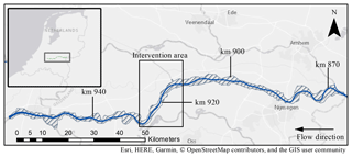
Our study domain covers the entire Waal River (Fig. 1). Distances along the river are measured using the conventional “Rhine kilometre”, which starts from km 0 at the German city of Konstanz. The Waal starts at km 867 at the Pannerden bifurcation and runs through to km 961 where it bifurcates in the Nieuwe Merwede and Boven Merwede rivers. All flood mitigation measures studied will be implemented between km 913 and 928, depicted by the annotated rectangle in Fig. 1.

The intervention area is characterised by a relatively straight river stretch with narrow floodplains and the strongly curved St. Andries river bend, which provides a known bottleneck during high discharges. Nine towns border directly on the dikes along this 17.5 km stretch. Interventions in this area to increase flood safety, considering the narrow floodplains and the populated surrounding land, present both a technical and a societal problem.

2.2 Hydrodynamic model & interventions

To simulate the hydrodynamic response of the flow to various interventions we use the Delft3D Flexible Mesh modelling system (Kernkamp et al., 2011). Geographical information, such as land cover, bathymetry and hypsometry, as well as information on embankments and weirs, was derived from the Baseline information system (Becker et al., 2014). Our setup uses a two-dimensional unstructured numerical grid, with between 71 000 and 120 000 active grid cells. The grid size varies from 40 m by 15 m in the main channel to a maximum of about 120 m by 120 m in the floodplains. In all cases, we simulate a steady upstream discharge of 10 165 m³ s⁻¹ and a constant downstream water level of 3.98 m + NAP (Normaal Amsterdams Peil), for 72 h. A single model evaluation on our computer resources took about 2.5 h. These conditions are consistent with a return period of 1250 years (T₁₂₅₀). Initial conditions were derived from a reference run with all considered stochastic variables (see Sect. 2.3) at their median values. The initial time step was set at 30 s.

All interventions are modelled as changes to a reference state of the system. This reference state is the Waal River after all interventions from the Room for the River programme, which approximately corresponds to the 2016 situation. We consider 12 additional system states, each one corresponding with a particular human intervention (Fig. 2). In all cases, the interventions were procedurally generated by the RiverScape tool (Straatsma and Kleinhans, 2018). We implemented six different interventions, detailed below. Each intervention was implemented in a low-intensity and a high-intensity variant. Here, intensity refers to the magnitude of the intervention, for example a small reduction in groyne height (low intensity) or a large reduction in groyne height (high intensity). We assume that the intervention is carried out in reality exactly as it was designed. This is known as the “as designed” post-intervention state. In reality, there may be a discrepancy between the as designed state and the actual (“as built”) state. In theory, this discrepancy could be considered an additional source of uncertainty. However, because there is no literature to support any assumptions regarding such a discrepancy, we do not take this into account here.

Figure 2 A schematic overview of a typical cross section of the River Waal and the flood mitigation measures studied in this paper. Figure is based on Middelkoop et al. (1999).

2.2.1 Groyne lowering (groynlow)

Groynes (also known as wing dikes or spur dikes) are (stone) structures perpendicular to the flow. During normal conditions, groynes restrict the effective channel width to promote navigable depths. However, during high flows groynes obstruct flow. Prior to 2016, many groynes in the Waal were already lowered as part of the Room for the River programme. The intervention as implemented in this study further reduces the groynes' crest heights. Groynes were lowered to the crest height corresponding to the water levels with exceedance frequency of 150 d (low intensity) and 363 d (high intensity) per year.

2.2.2 Minor embankment lowering (minemblow)

The River Waal floodplains are compartmentalised by minor embankments, of which original purpose is to prevent flooding of the floodplains during minor (summer) floods. This intervention lowers the crests of these embankments to reduce their obstruction during high flow. Low and high intensity lowered the crests to a water level with exceedance frequency of 50 d (low intensity) and 150 d (high intensity) per year.

2.2.3 Floodplain lowering (flplow)

Lowering or excavation of the floodplains increases the maximum water volume within the existing bounds of the river corridor, thereby increasing conveyance. In this study, we lower the level of the floodplain without changing existing vegetation or other floodplain configuration to isolate the effect of lowering. Floodplains were lowered to the corresponding water level with an exceedance frequency of 20 d yr⁻¹, with 5 % (low intensity) and 99 % (high intensity) of the terrestrial floodplain area altered.

2.2.4 Floodplain smoothing (flpsmooth)

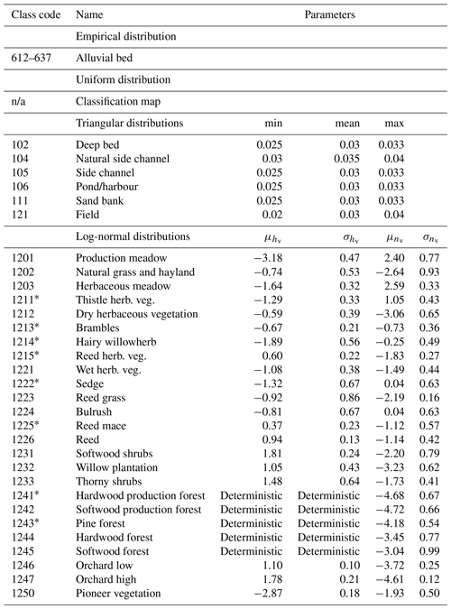
Vegetation in the floodplain greatly contributes to resistance during high flows. Replacing existing high-friction vegetation by low-friction vegetation mitigates this problem. Here, the existing vegetation was replaced by production meadow (roughness code 1201 in Table A1). Smoothing at low intensity affected the top 5 % of the obstructing vegetation. At high intensity all vegetation was converted to meadow.

2.2.5 Dike relocation (dikereloc)

In the River Waal, dikes are the primary defence against flooding. However, they also contribute to flood risk by restricting the river corridor. Dike relocation increases the floodplains and allocates more space to the river. While this is perhaps the best example of combatting problematic constriction of the river corridor, it is also the most invasive – considering human settlement near and on the dikes. At low intensity, concave dike sections of less than 700 m are replaced by straight dikes, whereas at high intensity concave sections of 7000 m are straightened, while creating small polders around existing built-up areas.

2.2.6 Side channels (sidechan)

Finally, the construction of secondary (side) channels within the existing corridor both increases the available volume and decreases vegetation friction. All new channels are assigned “side channel” roughness (code 105 in Table A1) and a trapezoidal cross sectional shape and slope of 1 to 3. The channels were implemented with widths of 10 m (low intensity) and 100 m (high intensity) and depths of 0.35 m (low intensity) and 3.5 m (high intensity) below the water level with an exceedance frequency of 363 d yr⁻¹.

2.3 Uncertainty sources

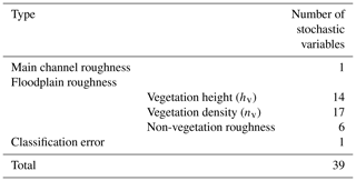
Modelling real-world rivers on the scale of nearly 100 km necessarily involves various simplifications, discretisations and parameterisations. Sources of uncertainty for this river were identified by Warmink et al. (2011) using expert elicitation. The main sources were (a) boundary conditions and (b) main channel friction and to a lesser extent (c) friction by vegetation, (d) geometry and (e) weir and groyne formulations. In this study we follow the design approach taken in the Room for the River programme, which assumes the boundary conditions are given and stationary for a certain design return rate (which is T₁₂₅₀) and therefore not a source of uncertainty. Warmink et al. (2013b) considered the hydraulic roughness parameters to be the most important parameter based on literature. We adopt this assumption and take uncertainty of the main channel friction, vegetation parameters and classification errors in the land-use maps into account. The total number of stochastic variables is 39 (see Table ).

Table 1 A summarised overview of the stochastic variables. A full overview is given in Table A1 in the Appendix.

2.3.1 Main channel roughness

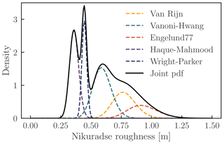
The hydraulic roughness of the main channel is chiefly determined by the material of the bed (“grain roughness”) and the bed forms (“form roughness”). Various models have been proposed that calculate the friction factor based on the characteristics of the bed (van der Mark, 2009). Here, we adopt the approach of Warmink et al. (2013a) who estimated the values for Nikuradse roughness height k_n (m) for a T₁₂₅₀ event by extrapolation using a generalised extreme value (GEV; Weibull variant) distribution for five roughness models. Given the GEV percentiles, we fitted a log-normal distribution at the T₁₂₅₀ return period for each roughness model. These log-normal distributions were combined into a single distribution using equal weight for each roughness model. Figure 3 shows the resulting individual and combined probability functions from the Weibull extrapolation.

In the following we will use the joint cumulative density function of the five roughness models to sample representative roughness height k_n. The joint cumulative function is a highly asymmetrical distribution, with a mean of approximately 0.58 m and 95 % confidence limits at 0.31 m and 1.0 m. The sampled values of k_n will be used in the hydrodynamic model as input for the White–Colebrook model:

$$\begin{array}{}\text{(1)}& C={\mathrm{18}}_{\mathrm{10}}\log {\displaystyle \frac{\mathrm{12}h}{k_{\mathrm{n}}}},\end{array}$$

with Chézy's coefficient C (m^1∕2 s⁻¹) and water depth h (m). The sampled k_n values are used to resolve friction for all main channel roughness classes, which cover 95.6 % of the main channel area. The other 4.4 % are non-erodible layers in the outer river bends which are not stochastically determined in this study.

Figure 3 The combined probability function of the main bed roughness is based on Weibull extrapolation of Nikuradse roughness height k_n to the T₁₂₅₀ return period using five different bed roughness formulas.

2.3.2 Floodplain roughness

The Baseline database divides the floodplain into vegetation classes, riverbanks and water bodies. Each class is given a specific roughness code called a trachytope, which is then coupled to an appropriate roughness formula and parameters specific to that formula. Spatially, the vegetation in the floodplains is discretised by polygons, which are designated by either one or a combination of distinct vegetation classes.

For vegetation, the generation of roughness by vegetation is complex, resulting from obstruction by stems and leafs and turbulent flow through the vegetation and over the canopy. The relationship between vegetation and roughness is extensively studied, leading to various models to compute hydraulic friction from vegetation traits (Nepf, 2012; Vargas-Luna et al., 2015; Shields et al., 2017). These traits often include the vegetation canopy height h_v (m), drag coefficient C_D [−], stem density n_v=m_vD_v or vegetation concentration $\mathit{\lambda }=\frac{\mathit{\pi }{D}_{\mathrm{v}}^{\mathrm{2}}{m}_{\mathrm{v}}}{\mathrm{4}}$, with the number of stems per square metre m_v (m⁻²) and stem diameter D_v (m) (Klopstra et al., 1997; Stone and Shen, 2002; Baptist et al., 2007; Huthoff et al., 2007; Yang and Choi, 2010; Li et al., 2015). Warmink et al. (2013b) have shown that the choice of a particular vegetation model has little influence on the outcome uncertainty compared to parameter uncertainty. Therefore, we only used the model proposed by Klopstra et al. (1997), in which vegetation friction is chiefly determined by the parameters $h_{\mathrm{v}},n_{\mathrm{v}},C_{\mathrm{D}}$. These parameter values are determined in the following way. For C_D we use fixed, deterministic values based on van Velzen et al. (2003). The height and density parameters (h_v and n_v) are assigned probability distributions based on the field campaign of Straatsma and Alkema (2009). Based on 206 field observations, they approximated the variation in vegetation density and height for 25 homogeneous vegetation classes. Based on their estimate quantiles we fitted log-normal distributions for each class, assuming the vegetation height and density to be independent parameters. In total, the roughness of 66 % of the River Waal floodplain is defined by one of the vegetation trachytopes, and 2.5 % is defined by the combination of two vegetation trachytopes.

Six trachytopes are associated with water bodies or riverbanks, accounting for about 27 % of the total areal. We model the friction for these six classes with the Manning formula:

$$\begin{array}{}\text{(2)}& C=h^{\mathrm{1}/\mathrm{6}}{n}^{-\mathrm{1}},\end{array}$$

with Manning's coefficient n (s m${}^{-\mathrm{1}/\mathrm{3}}$). The n values for these trachytopes are modelled as triangular probability functions with the minimum, maximum and mean values based on Chow (1959). All parameters of the vegetation parameter distributions are summarised in Table A1. The remaining 4.5 % of floodplain area, which is given deterministic roughness values, is mostly (3.7 %) covered by buildings which are excluded from flow computations, revetment and pavement.

2.3.3 Classification error matrix

Available vegetation maps are likely to contain “impurities” (Knotters and Brus, 2012) or classification errors, that have significant impact on model output uncertainty (Warmink et al., 2013a). The probabilities of one class being in reality another is encoded in a confusion matrix (we use Table 1 in Straatsma and Huthoff, 2011). Following this matrix it is found, for example, that “willow plantation” was, in all cases, found to be “softwood forest” instead. An overview of the various vegetation classes is given in the Appendix. Following these probabilities we generated an ensemble of 2000 pre-intervention trachytope maps. Each map was then given a fixed index number. We sample from these maps by picking a number from a discrete uniform distribution and finding the corresponding map by index number. In this way, each map is assigned the same probability.

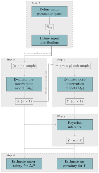
Figure 4 Schematic overview of the efficient uncertainty estimation method coral for post-intervention model output and impact analysis. In this figure, n represents the MCS sample size, m the subsample size, p the number of stochastic parameters, X the pre-intervention model output, j the number of draws from the posterior predictive model, Y the post-intervention model output, $\widehat{Y}$ the estimated post-intervention model output and ΔH the intervention effect. Figure is adapted from Berends et al. (2018).

2.4 Quantification of model output uncertainty

2.4.1 Estimation method

In this study we focus on prediction of the maximum flood levels (see Fig. 2) in the reference state (denoted by X), the maximum flood levels in the various interventions (denoted by Y) and the difference between these two (denoted by ΔH). Due to the uncertainties in model input discussed in Sect. 2.3, X, Y and ΔH are stochastic. To analytically compute differences between these two (stochastic) states of the river system, we would need to obtain both the model output probability distributions and the covariances between the two distributions (Berends et al., 2018). This problem is analytically intractable but can be solved numerically by Monte Carlo simulation (MCS; Metropolis, 1987; Stefanou, 2009). In the numerical approach, covariances are not explicitly computed.

However, MCS is not always practically feasible or desirable. Although MCS has been applied for estimation of flood level uncertainty before (Warmink et al., 2013b), the added task of performing a separate MCS for each intervention puts a severe strain on computational resources. Therefore we follow the approach of Berends et al. (2018), schematically depicted in Fig. 4, which is computationally more efficient. We refer to this method as “correlated output regression analysis” (coral). The key feature of coral is that the stochastic intervention output Y is not directly solved by MCS, but instead an estimator $\widehat{Y}$ is computed using the reference state and a correlation model. This correlation model is defined within a Bayesian framework and is probabilistic as well. We use the same linear model as Berends et al. (2018):

$$\begin{array}{}\text{(3)}& \widehat{Y}=\mathit{\alpha }(X-c)+\mathit{\beta }+\mathit{ϵ}+c,\end{array}$$

with $\mathit{ϵ}\sim \mathcal{N}(\mathrm{0},{\mathit{\sigma }}_{\mathit{ϵ}})$ and transformation constant c. The constant is introduced to shift data to the origin, which facilitates faster inference and is defined as $c=min\left(X\right)$. In the Bayesian framework, the regression parameters $\mathit{\theta }=\mathit{\{}\mathit{\alpha },\mathit{\beta },{\mathit{\sigma }}_{\mathit{ϵ}}\mathit{\}}$ are considered stochastic variables themselves and estimated via a Markov Chain Monte Carlo (MCMC) algorithm, trained by a limited subsample of simulations from Y. We use a subsample of m=20 for all intervention states. To estimate the distribution of the reference state (step 2) we use a quasi-random MCS sample (n=1000) with the Sobol low-discrepancy sequence. The linear model was demonstrated to be applicable to similar intervention studies by Berends et al. (2018), and (visual) inspection of the correlation between the reference state and the intervention models shows this holds for our cases as well.

The main advantage of this approach is a significant decrease of required computational resources by reducing the number of model evaluations. The total number of hydrodynamic model evaluations was 1240, divided over 13 model states (the reference plus 12 interventions). This is a decrease of computational effort of more than 90 % compared to direct MCS with all states, which would have totalled 13 000 model evaluations. It is important to state that the consequence of having a probabilistic correlation model is that the intervention state estimator $\widehat{Y}$ is stochastic for each individual draw from the reference state (X). Since X is stochastic itself, this can be thought of as the “uncertainty of the uncertainty” or the estimation uncertainty.

To maintain correlation between the X and Y, a union stochastic parameter space is constructed (step 1 in Fig. 4). Practically, this means that each corresponding member in the reference and intervention model ensembles has identical values for their stochastic variables, with the noticeable exception where those were altered by the intervention. For example, we assume that a tree with a height of 8 m in the reference case still has a height of 8 m after intervention, unless this tree was removed or otherwise affected by the intervention. This is straightforward to implement for parameter values but requires an additional step for the classification uncertainty. To be able to draw from the confusion matrix (see Sect. 2.3.3) a large number of trachytope maps was generated for the reference case. To maintain correlation, the same number of maps is generated for each intervention in such a way that every map is identical to the corresponding reference map with the same index, except in areas where the intervention has altered the trachytope. For example, an area which was classified as “willow plantation” in the reference state will still be classified as “willow plantation” after the intervention, unless that area has been reclassified as part of the intervention.

Figure 5 (a) Confidence levels of design water levels, normalised by the average water levels at each location. The water flow is from left (upstream) to right (downstream). The black line indicates km 893. (b) The histogram of the (not normalised) water levels at km 893.

2.4.2 Uncertainty metrics

As a data reduction step, we summarise the results using the following metrics based on the water level reduction effect ΔH.

Confidence intervals measure the distance between two percentiles (e.g. the 10 % and 90%) of a cumulative density function (cdf). We refer to the confidence intervals of the stochastic variables X, Y and ΔH as the model uncertainty confidence interval or MCI. For example, the MCI of ΔH is defined as

$$\begin{array}{}\text{(4)}& {\mathsf{\text{mci}}}_{\mathrm{\Delta }H}=\left|{\widehat{F}}_{\mathrm{\Delta }H}^{-\mathrm{1}}\right(p_{\mathrm{u}})-{\widehat{F}}_{\mathrm{\Delta }H}^{-\mathrm{1}}(p_{\mathrm{l}}\left)\right|.\end{array}$$

The MCI of $\widehat{Y}$ is derived in the same way. Here, ${\widehat{F}}^{-\mathrm{1}}$ is the inverse cumulative density function, also known as the quantile or percent point function and p_l, p_u the lower and upper quantiles. Here, these quantiles are always symmetric around the median. We use a limited subset of quantiles (consistent with the 10 %, 20 %, 50 %, 80 % and 90 % confidence intervals) to summarise the data. Additionally, we calculate the exceedance probability $P(\mathrm{\Delta }H<z)={\widehat{F}}_{\mathrm{\Delta }H}\left(z\right)$.

It is important to note that ${\mathsf{\text{mci}}}_{\widehat{Y}}$ and 𝙢𝙘𝙞_ΔH are stochastic – resulting from the estimation method. Therefore, each value belonging to an arbitrary quantile p_z may be expressed in terms of the expected value $E\left({\widehat{F}}_{\mathrm{\Delta }H}^{-\mathrm{1}}\right(p_z\left)\right)$ and variance $\mathrm{Var}\left({\widehat{F}}_{\mathrm{\Delta }H}^{-\mathrm{1}}\right(p_z\left)\right)$. This uncertainty may be referred to as the estimation uncertainty. A more detailed account of this can be found in Berends et al. (2018).

To compare the uncertainty of interventions we calculate the relative uncertainty, i.e. the uncertainty relative to the expected effect. For this, we use an adapted version of the coefficient of variation, defined as

$$\begin{array}{}\text{(5)}& U_{r;\mathrm{90}}={\displaystyle \frac{{\mathsf{\text{mci}}}_{\mathrm{90},\mathrm{\Delta }H}}{E\left(\mathrm{\Delta }H\right)}},\end{array}$$

where 𝙢𝙘𝙞_90,ΔH is the 90 % confidence interval for ΔH and E(ΔH) the average of ΔH. We use U_r;90 instead of the coefficient of variation (which is defined as the standard deviation on the expected value) to directly express the size of the largest used confidence interval in percentages of the expected effect. Therefore, a U_r;90 of 100 % means that the 90 % MCI is as large as the average effect. Since both 𝙢𝙘𝙞_90,ΔH and E(ΔH) are stochastic, U_r;90 is stochastic as well.

3 Results

3.1 Pre-intervention uncertainty

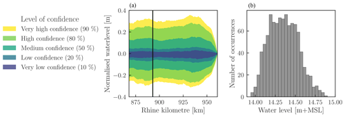
Figure 5 shows the uncertainty in the water levels along the River Waal before any intervention has taken place, normalised by the average water levels. The average confidence intervals over the entire stretch range from 55.4 cm for the 90 % interval to 5.7 cm for the 10 % interval. However, the intervals are not uniform along the river. At the downstream boundary the intervals collapse to zero due to the fixed boundary condition. Upstream from the boundary, there is a noticeably smaller interval, approximately between km 885 and 925. This is attributed to the relatively wider floodplains in this part of the river, which reduce flow through the main channel (Warmink et al., 2013b). The right-hand panel of Fig. 5 shows the histogram at km 893, which enables visual comparison with Fig. 6 in Warmink et al. (2013b), who performed their analysis with the WAQUA modelling system for the 1995 River Waal and slightly higher upstream boundary discharge. They reported a 95 % confidence interval of 68 cm (13.99 m + NAP to 14.66 m + NAP) at km 893. Our results also show a 95 % confidence interval of 68 cm, although at slightly higher water levels (14.05 m + NAP to 14.73 m + NAP). This provides confidence in the model results. However, we highlight two differences with respect to the study of Warmink et al. (2013b). First, we did not include the vegetation roughness model as a source of uncertainty, but we added vegetation parameter uncertainty. This change does not seem to have affected the output uncertainty of flood levels significantly. Second, the increase in flood levels with respect to the study of Warmink et al. (2013b) was not expected, given that between 1995 and 2015 a large-scale flood mitigation programme (Room for the River) was carried out aimed at reducing flood levels. However, given the different modelling systems and assumptions, this comparison cannot be used to judge the effectiveness of that programme.

Figure 6 The expected lowering of flood levels for side channel construction (a, sidechan) and floodplain smoothing (b, flpsmooth), with both high intensity and flow direction from left to right. The colours in this chart convey identical confidence levels as shown in Fig. 5. The location of the maximum expected effect is indicated by the dashed line and annotation x_m.

3.2 Uncertainty of along-channel flood level decrease

The primary objective of the flood mitigation measures is to lower flood levels during a given design discharge. In deterministic approaches, this effect is typically communicated with an along-channel diagram showing the difference (i.e. before and after the intervention) in flood levels (see, for example, Fig. 3 in Klijn et al., 2018). Figure 6 shows a similar diagram, augmented with information on the uncertainty of the prediction. The expected effect follows the general trend as a deterministic approach. Starting from the downstream end of the intervention (around km 932), water levels gradually decrease due to the local increase of conveyance compared to the reference state. From km 912 upstream, water levels gradually return to the reference equilibrium. The gradual relaxation to equilibrium levels both over and upstream from the intervention, i.e. backwater curves, is explained through basic subcritical flow theory. We note that the length of the backwater curves spans tens of kilometres, resulting in a residual water level decrease of approximately 5 cm near the upstream boundary (km 868). In theory, this could affect the distribution of discharge at the bifurcation of the River Waal with the Pannerden Canal. This secondary effect is not accounted for in this study.

The novelty of Fig. 6 results is mainly found in the uncertainty, visualised through the confidence intervals. These intervals follow the movement of the average, going down when the average decreases and relaxing toward the reference equilibrium upstream from the location of maximum effect (x_m). This shows that taking parameter uncertainty into account does not fundamentally change established typical effects of flood mitigation measures. However, the movement with the average is not accompanied by parallelity: the range of the intervals is not constant along the river. Instead, the range of the intervals scale with the expected effect: the ranges are small for small effects and increase with increasing effect. Consequently, uncertainty is largest at the maximum effect. Downstream from the intervention the confidence bands tend to zero, since for a steady computation, there is no difference between the pre- and post-intervention models and no backwater effects. Upstream from the intervention the confidence intervals reduce to zero along with the backwater curve effect.

Next, we compute the relative uncertainty (U_r;90) for each intervention and intensity. We first marginalise the uncertainty in U_r;90 due to coral by calculating the expected value (E(U_r;90)) for each point along the river (Fig. 7). Figure 7, as well as the relatively small standard deviations in Table 2, show that values for E(U_r;90) are fairly constant over the river length up to the location of the maximum flood level decrease (x_m) for all interventions. A notable exception is the peak at approximately km 885 for low-intensity groynlow. This is attributed to small inaccuracies in the estimation of the expected effect. Since U_r;90 is a ratio, its value is sensitive to small values of the denominator, which is the expected effect; see Eq. (5). groynlow has a very minor effect (maximum of 1 cm at low intensity), so small inaccuracies in estimation will greatly affect U_r;90. For this same reason, we do not compute U_r;90 upstream from the maximum effect, as the flood level decrease will rapidly return to and cross zero, which will lead to rapidly exploding U_r;90 values. From the fact that we do not observe such peaks much more often, we gain confidence that the chosen estimation method is suitable for this type of analysis even for very small-scale effects. In general, the constant values for E(U_r;90) show that it is a useful parameter to characterise the uncertainty of an intervention, as the increase in uncertainty with the effect, observed in Fig. 6, is sufficiently summarised by a single U_r;90 value.

It is interesting to note that in theory, the adaptation length (i.e. the length scale of the backwater curve) is affected by the equilibrium water level and can therefore result in converging or diverging confidence intervals. Since E(U_r;90) is relatively constant along the river, the adaptation lengths (i.e. the length scale of backwater effects) are not significantly affected by the intervention. Therefore, we see that all uncertainty is generated over the length of the intervention and subsequently diminishes upstream as water levels return to their equilibrium. In other words, if the adaptation lengths are known, the uncertainty upstream of x_m can be readily estimated from the relative uncertainty at x_m.

A comparison of all interventions (Table 2) shows that small effects ($E(\mathrm{\Delta }H{)}_{x_{\mathrm{m}}}$) are accompanied by small uncertainties ($E({\mathsf{\text{mci}}}_{\mathrm{90}}{)}_{x_{\mathrm{m}}}$). This shows that even small changes to rivers can be predicted, even when the absolute uncertainty in water levels (see Fig. 5) is an order of magnitude larger than the expected effect.

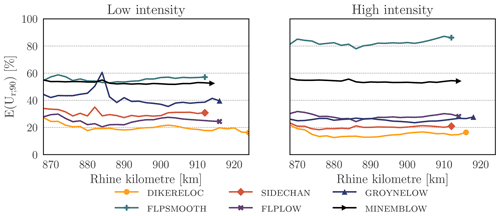
Figure 7 The expected values for the relative uncertainty (U_r;90) along the river, from the upstream boundary at km 868 to the location of maximum effect x_m indicated by the marker, showing relatively constant values upstream from x_m.

Table 2 Summarised results for each measure. H represents high intensity, L low intensity, x_m location given by Rhine kilometre (km) where maximum effect occurs, $E(\mathrm{\Delta }H{)}_{x_{\mathrm{m}}}$ expected effect at x_m, $E({\mathsf{\text{mci}}}_{\mathrm{90}}{)}_{x_{\mathrm{m}}}$ expected 90 % uncertainty at x_m, $\widehat{E\left(U_{r;\mathrm{90}}\right)}$ expected relative uncertainty along the river (average ± the standard deviation). The rows are sorted from highest expected effect (top) to lowest expected effect (bottom).

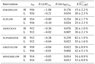
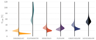
Figure 8 Probability densities of the relative uncertainty (U_r;90) at the location of maximum effect (x_m), for all interventions, showing that flpsmooth is significantly more uncertain than other interventions. Most interventions show similar distributions for the low-intensity (left, light-coloured) and high-intensity (right, dark-coloured) variants.

3.3 Inter-comparison between interventions

A straightforward way to compare differences between the effect of two or more interventions is to look at the backwater figures. In Fig. 6 we see two diagrams of interventions that result in flood level decrease within the same order of magnitude but with very different uncertainty. The uncertainty of flpsmooth is much higher than that of sidechan, as represented by the wider confidence intervals.

To systematically compare interventions we compute the relative uncertainty U_r;90 at the location of the maximum effect for each intervention (Fig. 8). Since U_r;90 is stochastic, we visualised the kernel density estimation of their probability distributions. In general we observe that (i) flpsmooth and minemblow are more uncertain than the other four interventions. This can be seen by their higher values for U_r;90, especially for the high-intensity variants. We also observe that overall, the low-intensity variants have similar distributions compared to their high-intensity variants, both in shape and location. Even in the cases in which the high-intensity variant distribution is clearly different from the low-intensity variant (dikereloc, groynlow and flpsmooth), the distributions still overlap. This shows that the intensity of an intervention is not a deciding explaining factor for U_r;90, even though it is evidently important in explaining the absolute uncertainty (𝙢𝙘𝙞₉₀) and the expected effect. The latter follows from the earlier observation that the absolute uncertainty scales with the expected effect following a (constant) relative uncertainty. For decision-making, it may be useful to estimate how much uncertainty is expected for a given expected effect. When considering different flood mitigation measures, the choice may depend on the level of acceptable uncertainty.

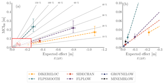
Figure 9 The expected effect (E(ΔH)) at x_m against the 90 % confidence interval, linearly interpolated between the low and high intensities. The relationship between the two is described by the relative uncertainty U_r;90, here shown as dashed grey lines. The error bars depict the estimation uncertainty (90 % interval). Panel (b) displays a zoomed-in part of the graph in (a).

By linearly interpolating between the expected values of the low and high intensities, we obtain a first approximation of the uncertainty for a given expected effect for each intervention (Fig. 9). For example, consider that the objective of a planned flood mitigation measure is 25 cm. We see from Fig. 9 that this can be accomplished by four different interventions (flpsmooth, flplow, sidechan and dikereloc), within the bounds marked by the low and high intensities. The confidence intervals differ markedly between these choices. Under the assumption of linear interpolation between the two intensities, the 90 % confidence intervals for an expected decrease of 25 cm are estimated at 4 cm (dikereloc), 5 cm (sidechan), 7 cm (flplow) and 21 cm (flpsmooth). These intervals may or may not be acceptable.

Instead of looking at the expected effect, the confidence intervals can be marginalised by designing for a given exceedance probability of the effect. The desired effect is related to the expected effect through the exceedance probability. To illustrate how the exceedance probability can be used to guide intervention design, we linearly interpolated between the low-intensity and high-intensity variants as a function of the expected effect (Fig. 10). In this figure, the estimation uncertainty is not taken into account. Given that we only have two points (low and high intensity), a linear transformation is the only model we can support. Although we acknowledge that other models are possible, we included this as a first approximation because it illustrates information available for decision makers.

The high-intensity variant of flpsmooth has an expected flood level decrease of 28 cm. However, the likelihood that the decrease is smaller (or higher) than that number is only approximately 50 %. This means that the expected effect of 28 cm is as likely as not to be met by the proposed intervention. In contrast, the 90 % exceedance probability for the high-intensity variant is 18.7 cm. This means that it is “very likely” (following IPCC terminology; see Solomon et al., 2007) that the flood level decrease is larger than 18.7 cm.

This approach can be applied to the earlier example of a planned mitigation measure with a 25 cm flood level decrease objective. In Fig. 10b, we see that at an exceedance probability of 66 % (“likely”), all four possible interventions can be implemented. However, to meet this likelihood all interventions have to be “over-designed”, i.e. meet a larger expected flood level decrease than the given objective. For example, floodplain smoothing needs to be designed for an expected effect of 28 cm for a 66 % likelihood of reaching the objective of 25 cm. The amount by which the measure needs to be over-designed depends on the uncertainty of that measure and the exceedance probability. Higher exceedance probabilities such as a 95 % likelihood (“Extremely likely”) can also preclude some flood mitigation measures (Fig. 10c). With this level of confidence, flpsmooth can no longer be considered: none of the computed examples reach an “extremely likely” flood level decrease of 25 cm within the limits of the considered interventions. In this case, there is a physical limit to an even higher intensity flpsmooth, since there is simply no more available land within the study area to turn into meadow. Extrapolation beyond the given limits is therefore not possible, although a higher effect could be obtained by simply enlarging the study area. Within the given limits, the three remaining interventions (dikereloc, sidechan and flplow) can still be used. They would need to be designed for an expected effect of −0.27, −0.28 and −0.29 m, respectively. For perspective, it is worth pointing out that one of the greatest interventions on the River Waal in the past decades, the Nijmegen–Lent dike relocation project, has (deterministically) predicted effect of −27 cm, at an estimated cost of more than EUR 10 million per cm flood level decrease.

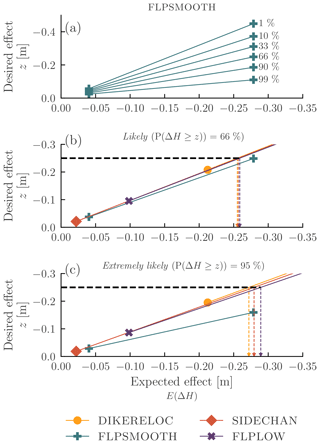
Figure 10 (a) The relationship between the expected effect E(ΔH) and the exceedance level z for various exceedance probabilities. (b) Inter-comparison of a 66 % exceedance probability for four interventions. The dashed black line indicates a z of 25 cm, and the coloured dashed lines indicate which expected levels belong to that z, given the exceedance probability (see text). (c) Same as (b) but for an exceedance probability of 99 %. Note that all lines show the expected value of the exceedance level; the estimation uncertainty is not depicted.

4 Discussion

Our results show that some interventions are inherently more uncertain than other interventions. Given the complexity of high-detailed modelling of floodplains, it is not straightforward to explain these differences. The statistical causes of uncertainty are discussed in detail by Berends et al. (2018). They observed that the removal of existing stochastic elements (e.g. a vegetation polygon) in exchange for new ones greatly increased the unexplained variance (ϵ in Eq. 3) and therefore increases effect uncertainty. We see that here as well: flpsmooth, which removes high-friction vegetation in exchange for meadow, is by far the most uncertain intervention. However, in this study we have argued that the relative uncertainty (U_r;90) is a more useful parameter than the absolute uncertainty (mci). In that context, a large absolute uncertainty can be offset by a large expected flood level decrease. This is evidenced by both dikereloc and flplow, which both have a large absolute uncertainty at high intensity but a relatively low relative uncertainty. A reduction in relative uncertainty could therefore be achieved by minimising the amount of change to existing floodplains while optimising the expected flood level decrease. This general observation is likely applicable to other rivers and case studies.

A lack of computational resources is often named as the main obstacle that motivates the use of deterministic approaches over probabilistic approaches. The analysis performed in this study is nonetheless feasible due to the coral approach, which reduces the required computer resources by reducing the number of model evaluations. An additional advantage of this method is that the uncertainty of the estimation is known and can be explicitly incorporated in analyses. In this study, we show that the relative uncertainty U_r;90 can be estimated to a sufficient precision (Fig. 8) to draw conclusions, even with a relatively low number of model runs (20 for each intervention). It is possible to decrease the estimation uncertainty by increasing the number of model runs with the post-intervention models (Berends et al., 2018), if (computational) resources allow.

Our study focused on providing uncertainty estimations for many different interventions, not on providing an optimal intervention for the given case study. Following this approach we made several simplifications that must be resolved if an optimal intervention design is pursued. The linear interpolation between low-intensity and high-intensity interventions in Figs. 9 and 10 was used to obtain a first approximation of the uncertainty for interventions at different intensities. These figures are useful to illustrate how confidence levels and differences in relative uncertainty between interventions affect the expected effect but should not replace new calculations in intervention design – in part because our study provides only two support points, which is insufficient to either support or oppose the assumption of linearity. Rather, they may help to provide a starting point for a new set of calculations. Second, we marginalised the estimation uncertainty in Fig. 10 by averaging, to show how model uncertainty implicates intervention design. Practical use of exceedance levels should include estimation uncertainty of those levels – which can be reduced by increasing the number model evaluations if necessary. Finally, the interventions studied in this paper are single archetypes, while in reality designs would likely be a combination of multiple archetypes (e.g. side channel combined with lowering of the surrounding floodplain). Our study does not provide support for claims regarding such compound interventions, which would require further study.

Our approach is a form of forward uncertainty analysis: the quantification of model output uncertainty based on uncertainty in model assumptions without taking historical evidence of the goal variable (i.e. water level measurements) into account. We justify choosing this approach based on the assumption that no historical information can be used to infer or narrow the distributions of the uncertain parameters because (a) such information does not exist for our study case, and (b) measurements after the intervention will never be available ex ante. The results of our analysis are therefore conditional on our assumptions about the validity of the model, the selection of uncertainty sources and the probability distributions of these sources. We have taken care to select the stochastic variables, and their distributions, based on previous research specific to our study case. Forward uncertainty analysis is contrasted (e.g. see Beven et al., 2018) with so-called inverse methods, such as GLUE (Beven and Binley, 2014), DREAM (Vrugt et al., 2008) or deterministic calibration, that use historical evidence to potentially narrow the uncertainty bands of input variables. However, the potential use of historical data to constrict uncertainty faces complex challenges which will have to be met. Chief among them are extrapolation to unmeasured conditions and dealing with the large number of uncertain variables (here, 39) which may not be uniquely identifiable (Werner et al., 2005). In any case, like traditional deterministic approaches, the assumptions underlying probabilistic approaches should be readily available, transparent and open to discussion.

Models can play a role in decision support under (deep) uncertainty, and the uncertainty quantification is an important step to model the future (Maier et al., 2016). However, too much focus on quantifiable uncertainty should be avoided. Warmink et al. (2017) documented several examples in which too much focus on quantifiable (also “statistical” or “technical”) uncertainty resulted in knowledge creation that did not contribute to the policy process (“superfluous knowledge”). A key idea is that other uncertainties exist that cannot be reduced by more data or simply cannot be quantified. Examples of these include “social uncertainty”: fundamental disagreement between experts, lack of trust in scientific results, ambiguity and diverging narratives based on the same empirical basis (Sarewitz, 2004; Brugnach et al., 2011; Warmink et al., 2017). Coping with such uncertainties may require adaptive river management (Pahl-Wostl, 2009) and exploration of multiple alternate futures (see the third paradigm of  Maier et al., 2016, and references therein). Given these considerations, there are several probabilistic frameworks of flood risk adaptation strategies to which explicit quantification of model uncertainty is a natural and required extension (e.g. Lendering et al., 2018; Klijn et al., 2018). In this paper, we demonstrated that model predictions of human intervention in rivers are sensitive to uncertainty and can substantially influence design decisions. Therefore, we argue that trusting only in the best available knowledge and, by extension, prediction by the best-available models, is not sufficient for planning interventions in river systems. Finally, our study was limited to the effect of interventions with respect to water level lowering. We did not consider other indicators, such as economic, ecological or societal costs and benefits, as was done by Straatsma et al. (2019) (albeit without addressing uncertainty). Multidisciplinary and multi-sectoral assessment of interventions including uncertainty is recommended to determine trade-offs in river management. coral provides a computationally effective method to do so.

5 Conclusions

In general, our study shows that explicitly quantifying the uncertainty of predicted flood mitigation measures provides decision makers and modellers with valuable information. On the one hand, results show how taking uncertainty into account can lead to different design choices. On the other hand, even small effects on flood levels can be quantified because small effects are accompanied by small uncertainties. This shows that model uncertainty does not invalidate model-supported decision-making in river management, but it enriches it.

Our first objective was to quantify the effect of parameter uncertainty on the predicted effectiveness of flood mitigation measures. Based on previous studies, we quantified the parameter uncertainty for 39 variables and estimated the uncertainty of model output. Results show that the absolute uncertainty of the predicted effect of flood level decrease is highly dependent on the type of intervention and location along the river. However, we found that the confidence bounds of flood level decrease along the river can be adequately described by a single relative uncertainty metric, defined as the ratio between the 90 % confidence interval and the expected effect. This ratio remains relatively constant along the river and between intensities of intervention types and enables us to make some general observations. First, all uncertainty is “generated” when the intervention has modified the river system. Upstream from there, the uncertainty gradually diminishes upstream with a constant rate following typical backwater curves. Second, a higher expected flood level decrease led to a higher uncertainty, and a small flood level decrease was accompanied by a small uncertainty. The ranges of the expected relative uncertainty varied between 15 % and 40 % for most interventions, which means that the size of the 90 % confidence bounds of those interventions is less than half of the expected flood level decrease.

The second objective was to explore the relationship between the expected effect and its uncertainty, to aid in the decision-making process. We observe that interventions of different types may reach the same expected flood level decrease but have different uncertainty. Specifically, a large-scale but relatively ineffective intervention such as floodplain smoothing (by removing high-friction vegetation) has a high relative uncertainty compared to alternative interventions. The intensity of an intervention (e.g. total area of vegetation smoothed) may be increased to reach a higher effect. Our results show that higher intensity also leads to a higher uncertainty, while the relative uncertainty remains approximately constant. This relationship was then used to show how explicit uncertainty quantification and differences in relative uncertainty between various interventions may affect design choices, depending on the level of acceptable uncertainty. For a fixed level of acceptable uncertainty (i.e. by a given exceedance probability), we graphically demonstrated that interventions need to be designed for a larger expected flood level decrease than the given objective.

Appendix A: Parameter distributions for vegetation types

Table A1 Parameters of the floodplain roughness class distributions. Codes marked with an asterisk ^∗ are not used in the Waal model. “n/a” stands for “not applicable”.