the Creative Commons Attribution 4.0 License.
the Creative Commons Attribution 4.0 License.
 | 14 Nov 2018
Temporal evolution of flow-like landslide hazard for a road infrastructure in the municipality of Nocera Inferiore (southern Italy) under the effect of climate change
Marco Uzielli
Guido Rianna
Fabio Ciervo
Paola Mercogliano
Unni K. Eidsvig
In recent years, flow-like landslides have extensively affected pyroclastic covers in the Campania region in southern Italy, causing human suffering and conspicuous economic damages. Due to the high criticality of the area, a proper assessment of future variations in event occurrences due to expected climate changes is crucial. The study assesses the temporal variation in flow-like landslide hazard for a section of the A3 “Salerno–Napoli” motorway, which runs across the toe of the Monte Albino relief in the Nocera Inferiore municipality. Hazard is estimated spatially depending on (1) the likelihood of rainfall-induced event occurrence within the study area and (2) the probability that the any specific location in the study area will be affected during the runout. The probability of occurrence of an event is calculated through the application of Bayesian theory. Temporal variations due to climate change are estimated up to the year 2100 through an ensemble of high-resolution climate projections, accounting for current uncertainties in the characterization of variations in rainfall patterns. Reach probability, or defining the probability that a given spatial location is affected by flow-like landslides, is calculated spatially based on a distributed empirical model. The outputs of the study predict substantial increases in occurrence probability over time for two different scenarios of future socioeconomic growth and atmospheric concentration of greenhouse gases.
- Article
(7483 KB) - Full-text XML
- BibTeX
- EndNote


In recent years, eminent scholars have debated about the main features of “shallow” and “deep” uncertainties in the assessment of natural hazards (Stein and Stein, 2013; Hallegatte et al., 2012; Cox, 2012). Shallow uncertainties are associated with reasonably knowing the probabilities of outcomes (Stein and Stein, 2013), while deep uncertainties are associated with (1) several possible future worlds without known relative probabilities, (2) multiple conflicting but equally reasonable world views, and (3) adaptation strategies with remarkable feedbacks among the sectors (Hallegatte et al., 2012).
As stressed in these works, climate change and its impacts can be considered paradigmatic of very deep uncertainty. Given the extent of potential impacts on communities (United Nations, 2015), including their economic dimension (Stern, 2007; Nordhaus, 2007; Chancel and Piketty, 2015), considerable effort has been made in recent years to assess the variations in frequency and magnitude of weather-induced hazards in a changing climate (Seneviratne et al., 2012). A variety of strategies have been devised and implemented with the aim of detecting the main sources of uncertainty and their extents (Wilby and Dessai, 2010; Cooke, 2014; Koutsoyiannis and Montanari, 2007; Beven, 2015).
Investigations of future trends in the occurrence and consequences of weather-induced slope movements and of the uncertainties in their estimation have received relatively limited interest (Gariano and Guzzetti, 2016; Beven et al., 2018). The paucity of investigations could be due to the mismatch between the usual scale of analysis for landslide case studies and the much coarser horizontal resolutions of climate projections currently available as well as the difficulty in generalizing findings to other contexts, given the relevance of site-specific geomorphological features.
1.1 Previous studies of flow-like movements in pyroclastic soils in Campania
In an attempt to address the above limitations, several recent studies have focused on future variations in the occurrence of flow-like landslides, or more generally, flow-like movements affecting pyroclastic covers mantling the carbonate bedrock in the Campania Region in southern Italy. Flow-like movements in granular materials such as pyroclastic terrain are among the most destructive mass movements due to their velocity and the absence of warning signs (Hutchinson, 2004; Cascini et al., 2008).The aforementioned studies focused on a number of sites, namely Cervinara (Damiano and Mercogliano, 2013; Rianna et al., 2016), Nocera Inferiore (Reder et al., 2016; Rianna et al., 2017a, b), and Ravello (Ciervo et al., 2016). Several aspects differentiate the case studies and, consequently, the respective investigations. The depth, stratigraphy, and grain size of pyroclastic covers are fundamentally regulated by slope, distance to volcanic centers (Campi Flegrei and Somma-Vesuvio), and the wind direction and magnitude during the eruptions; therefore, the critical rainfall pattern inducing the slope failure varies according to these differences (e.g., intensity and the length of antecedent precipitation time window). Indeed, at some locations (Cervinara and Nocera Inferiore), the triggering event is recognized as being characterized by daily duration (also acting jointly with wet antecedent conditions), while in other locations (Ravello), events in shallower covers or covers formed by coarser materials require heavy rainfall lasting several hours. Consequently, two different approaches are followed (for the scope of such a data elaboration) based on the considered duration. Relative to daily durations, the former modifies daily observations according to projected anomalies (Damiano and Mercogliano, 2013) or simulated data through statistical bias correction approaches (adopted for the Cervinara and Nocera Inferiore test cases). In the latter case, a stochastic approach is coupled with bias-corrected climate data to provide assessments at an hourly scale (adopted for the Ravello test case). Some studies (Reder et al., 2016; Ciervo et al., 2016; Rianna et al., 2017b) make use of expeditious statistical approaches referring to rainfall thresholds to assess slope stability conditions, while other studies employ physically based approaches (Damiano and Mercogliano, 2013; Rianna et al., 2017a).
1.2 Objective of the study
This study focuses on the quantitative estimation of the temporal evolution of hazard for rainfall-triggered flow-like movements affecting a stretch of a national motorway in the municipality of Nocera Inferiore. Flow-like landslide runout is probabilistically investigated through a frequentist estimate of “reach probability” (Rouiller et al., 1998; Copons and Vilaplana, 2008) performed in a GIS environment, thus allowing for the seamless mapping of landslide hazard under current and future climate change scenarios.
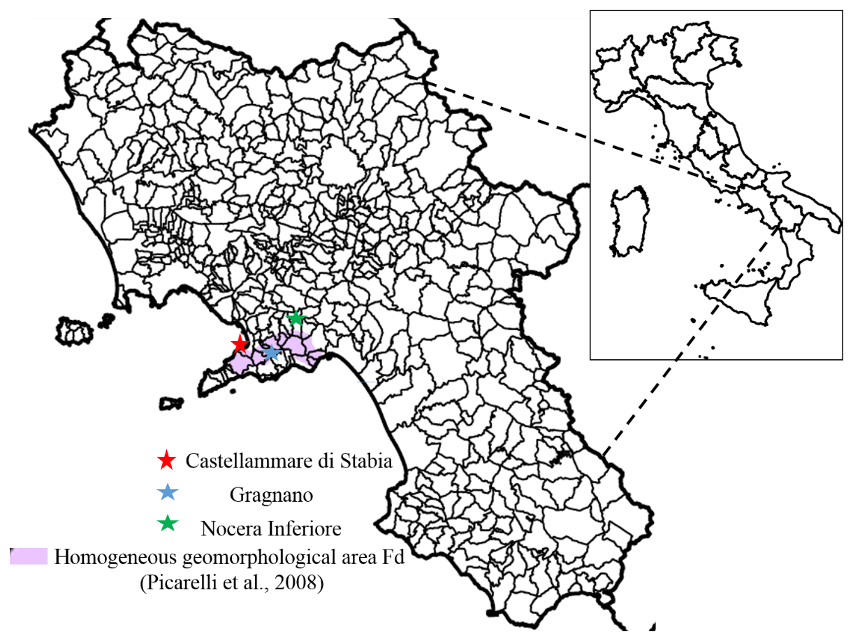
The study presents significant elements of novelty. For instance, through a Bayesian approach, it characterizes precipitation values cumulated for two time windows as proxies for the triggering of flow-like movements in pyroclastic covers in the Lattari mountain range. The resulting quantitative model returns temporal variations in triggering probability, thus accounting for the effect of climate change on rainfall trends. Uncertainties in variations in rainfall patterns are taken into account by means of the EURO-CORDEX ensemble. Projections provided by climate simulations are bias-adjusted, allowing for the comparison with available physically based rainfall thresholds while adding further assumptions and uncertainties in simulation chains. The analysis also relies on rainfall data from the rain gauges located in Gragnano and Castellammare di Stabia. The location of the three towns in Italy and in the Campania region is illustrated in Fig. 1.
2.1 Geographic and geomorphological description
Most of the territory of the Nocera Inferiore municipality belongs geomorphologically to the Sarno River valley. The most urbanized area of the town is located at the toe of the northern slopes of the Mount Albino relief, pertaining to the Lattari mountain range (Fig. 2, sector A); other more sparsely populated areas are located at the foot of the Torricchio hills (Fig. 2, sector B). These reliefs are constituted by carbonate rocks covered by air-fall pyroclastic deposits originating from volcanic eruptions (Somma-Vesuvio complex) during the last 10 000 years (Pagano et al., 2010). Such covers in loose pyroclastic soils have historically been affected by multiple types of rainfall-induced flow movements, including Gragnano (in 1997), Sarno and Quindici (in 1998), Nocera (in 2005), and Ischia (in 2006). The complete list of events affecting the area considered in the study in the period 1960–2015 is given in Table 2. Movement types include (a) “hyper-concentrated flows” (flows in the transition from mass transport to mass movement) that are generally triggered by washing away and/or progressive erosive processes along rills and inter-rill areas, (b) “channelized debris flows” (channelized flow-like mass movements) that are generated by slope failure in “zero order basin” (ZOB) areas (Dietrich et al., 1986; Cascini et al., 2008) and funnel into stream channels (the propagation process is laterally confined by the stream channel), and (c) “un-channelized debris flows” (un-channelized flow-like mass movements; Costa, 1984; Hutchinson et al., 2004), which are locally triggered on open-slope areas and propagate as debris avalanches (the propagation process is not laterally confined). The third type characterized the most recent event that affected the town in March 2005, causing three fatalities and extensive damage to buildings and infrastructure (Pagano et al., 2010; Rianna et al., 2014). This study focuses specifically on a section of the A3 “Salerno–Napoli” motorway, which runs across the toe of the Monte Albino relief, as shown in Fig. 3.
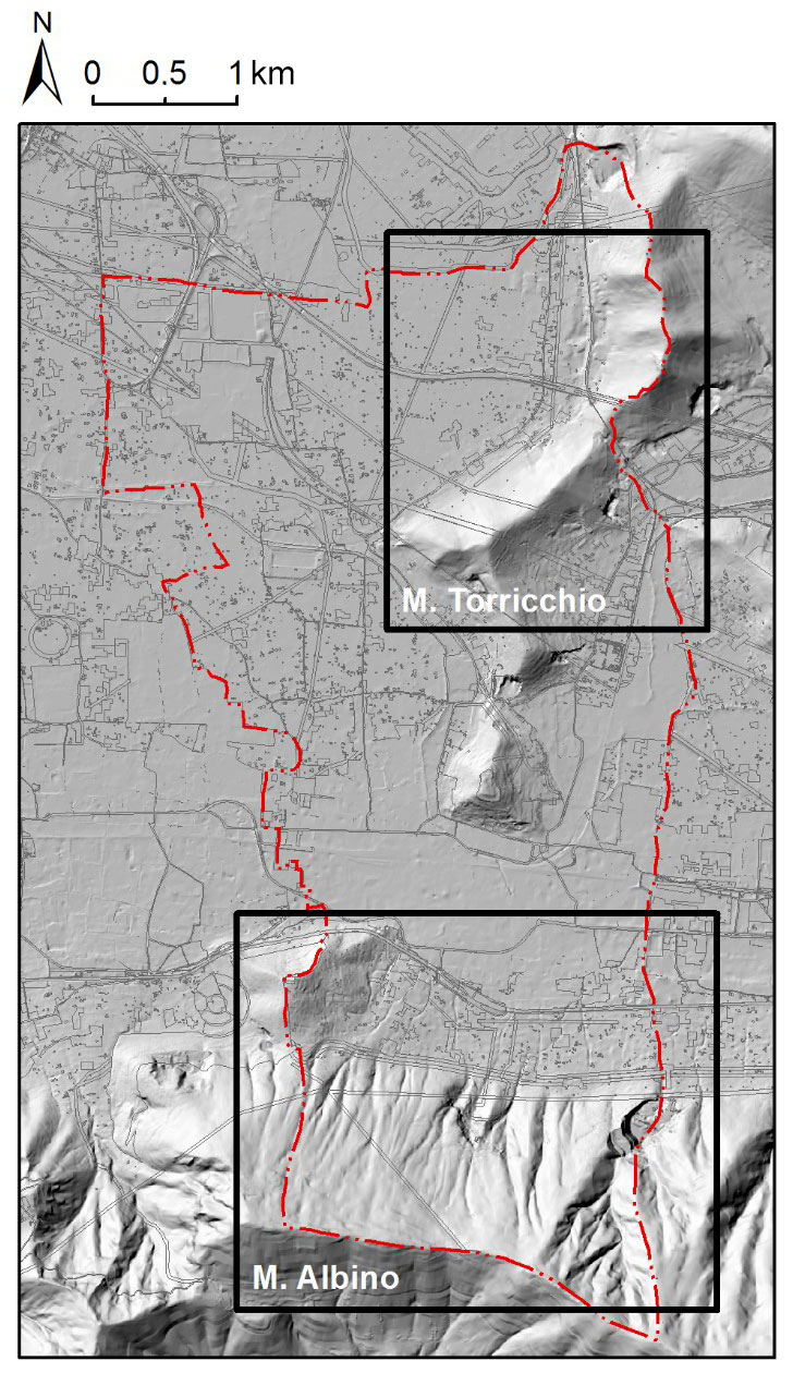
Figure 2Geomorphologic setting and administrative boundaries of the Nocera Inferiore municipality.
In the disaster risk management discipline, the term “hazard” has been linked to multiple definitions and operational guidelines, depending on the scope, technical approach employed, and available data and models. Fell et al. (2008) distinguish “susceptibility zoning” from “hazard zoning” on the basis that the former involves the spatial distribution and rating of the terrain units according to their propensity to produce landslides, while the latter should include, wherever possible, the quantitative estimation of the frequency of landsliding. In situations where this estimation is difficult to pursue, some approximate guidance on frequency should be provided. Corominas et al. (2015) defined hazard as “a condition that expresses the probability of a particular threat occurring within a defined time period and area”, with no explicit reference to frequency. In this study, calculated hazard levels refer to the frequency of the occurrence of at least one landslide event within the study area in 30-year periods. In the more specific context of the case study presented herein, the geologic hazard mapping web page of ISPRA, the Italian National Institute for Environmental Protection and Research, states that landslide prediction models “usually address where an event is expected to occur and with which probability, without explicitly estimating return periods and intensities”.
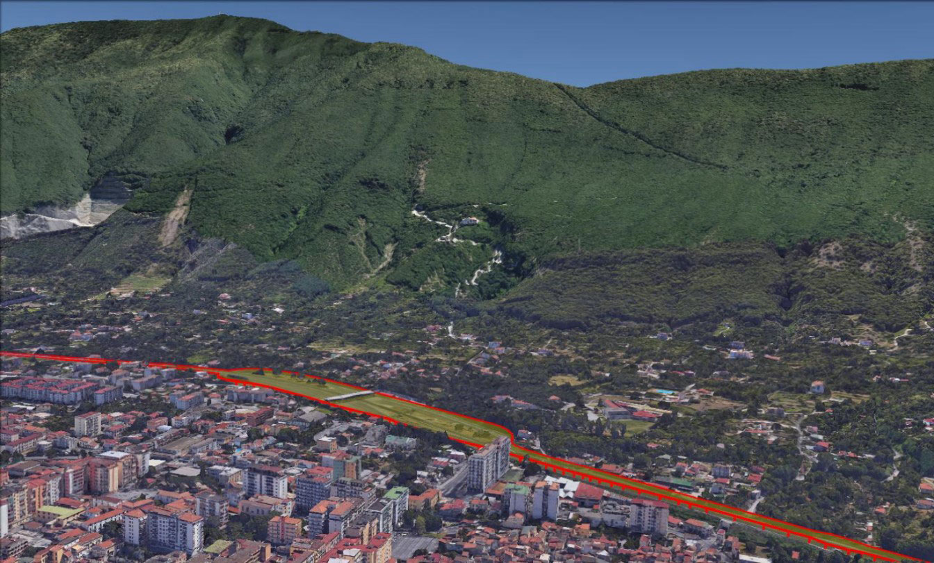
Figure 3Infrastructure-scale view of the study area with the A3 Salerno–Reggio-Calabria motorway (boundaries marked in red).
Operationally, the study is conducted by coupling mathematical software with GIS to obtain spatially referenced estimates of hazard and its mapping. A digital terrain model (DTM) of the study area, having a resolution of 15×15 m, was built for the purpose of the GIS-based modeling of runout. The original resolution adopted for the Campania region's ORCA project in 2004 was 5×5 m. A variety of DTM resolutions were tested for the case study. The adopted resolution proved to be sufficient to adequately represent the surface morphology and runout as detailed in Sect. 6. Hazard is estimated quantitatively for each cell in the GIS-generated grid through the following model:
where PL is the probability of event occurrence and PR is the reach probability for the cell. Occurrence probability defines the likelihood of the occurrence of at least one event in the study area as a consequence of the attainment of given thresholds of cumulative rainfall and of the likelihood of triggering given the occurrence of such thresholds. Reach probability describes the probability that a given cell will be reached by a moving soil mass, assuming that flow-like landslides have been triggered in one or more potential source areas. Occurrence probability and reach probability are distinct parameters that depend on different factors and are computed separately.
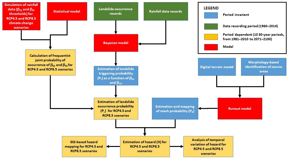
Occurrence probability is partly related to the likelihood of triggering given the attainment of specific rainfall thresholds, which is assumed to be an inherent, time-invariant attribute of the area, and it is partly related to climate change through the time-dependent probability of the exceedance of such rainfall thresholds, as described in Sect. 5. Reach probability is not related to climate change, as it parameterizes the probability of spatial occupation during runout, assuming that triggering has occurred. Reach probability depends solely on terrain factors and is thus amenable to the concept of susceptibility, as defined by Fell et al. (2008), among others. Occurrence and triggering probabilities are related to rainfall parameters and, thus, are assumed to be spatially invariant and uniform for the entire area (but are time-dependent), while reach probability depends on geomorphological factors and is thus cell-specific and spatially variable (but is time-invariant) within the area. These aspects are explained in detail later in the paper. The study is conducted according to the operational flowchart shown in Fig. 4. The modular approach initially involves the disjoint estimation of occurrence probability (including its temporal variation), as described in Sect. 5, and of reach probability, as detailed in Sect. 6. Subsequently, hazard is calculated in Sect. 7 using the model described above.
4.1 Observed precipitation data
Observed datasets are used to identify time windows used as proxies for flow-like landslide triggering to implement the Bayesian approach described in Sect. 5.2. Subsequently, data from the Nocera Inferiore station are used for the bias adjustment of climate projections estimating occurrence probability (Sect. 5.3). Although the study focuses on Nocera Inferiore flow-like movements, data from the neighboring towns of Gragnano and Castellammare di Stabia are considered in order to increase the size of the event database, thus increasing the statistical significance of the approach. At both sites, events affecting pyroclastic covers were observed to be very similar to those of the Nocera Inferiore slopes (De Vita and Piscopo, 2002) as described in Sect. 4.2.
The dataset related to daily precipitation spans across the time window from 1 January 1960 to 31 December 2015. Unfortunately, no weather stations were in operation throughout the entire period for any of the three towns. Consequently, the dataset was reconstructed by merging data provided by different weather stations. Prior to 1999, the network of monitoring stations was managed by Servizio Idrografico e Mareografico Nazionale (SIMN – Hydrographic and Tidal National Service) network at the national level. In that period, the selected reference weather station is that which is located within the town and is identified with the town's name, as can be found in the SIMN yearbooks. Subsequently, the management was delegated to regional level, with the regional civil protection managing the dataset for the Campania region. Since 1999, the reference weather stations have been selected as some of those adopted for the towns in regional early warning systems against geological and hydrological hazards (2005). Checks for the homogeneity of time series and for the unwarranted presence of break points between the two periods were carried out for this study through the Pettitt (1979) and CUSUM (CUmulative sum; Smadi and Zghoul, 2006) tests. Source weather stations, their locations, installation times, and main (i.e., at least 4 months in a year) out-of-use periods are reported in Table 1.
Table 1Weather stations used in the compilation of datasets for Nocera Inferiore, Gragnano, and Castellammare di Stabia and their locations, installation times, and main out-of-use periods.
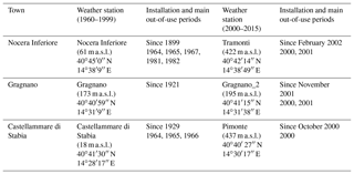
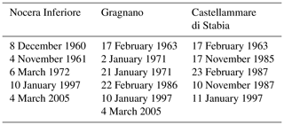
Table 2Flow-like mass movements affecting pyroclastic covers in Nocera Inferiore, Gragnano, and Castellammare di Stabia in the period 1960–2015.
4.2 Flow-like movements inventory
The inventory was compiled using three main references: Vallario (2000), De Vita and Piscopo (2002), and, for the more recent events, the “Event Reports” drafted by the regional civil protection. The multiple sources used for reconstructing the inventory provide quite different details. De Vita and Piscopo (2002), for example, report the cumulative rainfall values inducing the events on time spans up to 60 days for events in the same geomorphological context. Vallario (2000) provides brief descriptions about the events (also for the other natural hazards affecting the region), including the number of fatalities and injured people. “Event Reports”, drafted by the regional civil protection, contain exhaustive descriptions about the weather patterns inducing the triggering event and the main consequences for the affected communities. It is worth recalling that only events affecting pyroclastic covers have been considered and included in the dataset. Sixteen events were observed in the period 1960–2015, as detailed in Table 2.
4.3 Climate projections
The generation of climate projections was conducted for Nocera Inferiore as a preliminary step in the quantitative characterization of the temporal evolution of occurrence probability, since the latter depends partly on the frequency with which specific rainfall thresholds are attained. The adopted simulation chain includes several elements. Firstly, scenarios about future variations in the concentrations of atmospheric gases inducing climate alterations are assessed through socioeconomic approaches including demographic trends and land use changes. IPCC (Intergovernmental Panel on Climate Change) defined Representative Concentration Pathways (RCP) in terms of increases in radiative forcing in the year 2100 (compared to preindustrial era) of about 2.6, 4.5, 6.0, and 8.5 W m−2. Such scenarios force global climate models (GCM). These are recognized for their reliable representation of the main features of the global atmospheric circulation but fail to reproduce weather conditions at temporal and spatial scales of relevance for assessing impacts at the regional and local scale. In order to bridge such a gap, GCMs are usually downscaled through regional climate models (RCMs). These are climate models nested on GCMs, from which they retrieve initial and boundary conditions, but work at higher resolutions (including a non-hydrostatic formulation) on a limited area. The dynamic downscaling from GCMs to RCMs allows for a better representation of surface features (orography, land cover, etc.) and of associated atmospheric dynamics (e.g., convective processes). Nevertheless, persisting biases can hinder the quantitative assessment of local impacts.
In order to cope with such shortcomings, a number of strategies can be adopted. For instance, to characterize uncertainty associated to future projections, a climate multi-model ensemble can be utilized where different combinations of GCM and RCM run on fixed grid and domain. Furthermore, statistical approaches (e.g., Maraun, 2013; Villani et al., 2015; Lafon et al., 2013) can be pursued to reduce biases assumed as systematic in simulations. More specifically, quantile mapping approaches have been applied for impact studies with satisfactory results in recent years. In these applications, the correction is performed to ensure that “a quantile of the present-day simulated distribution is replaced by the same quantile of the present-day observed distribution” (Maraun, 2013). However, limitations and assumptions associated to these approaches should be clear to practitioners (Ehret, 2012; Maraun and Widmann, 2015).
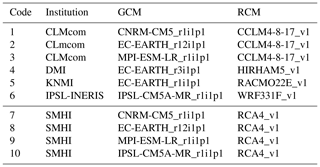
In the present study, climate simulations included in EURO-CORDEX multi-model ensemble at 0.11' (approximately 12 km) are considered under the RCP4.5 and RCP8.5 scenarios, as described in Table 3 (Giorgi and Gutowski, 2016). Climate simulations are adjusted for bias through an empirical quantile mapping approach (Gudmundsson et al., 2012) using data from Nocera Inferiore weather stations from the period 1981–2010.
In Fig. 5, the variations expected in monthly cumulative values (5a) and maximum daily precipitation (5b) are displayed, assuming 1981–2010 as the reference period and splitting the period 2010–2100 into three 30-year periods. More specifically, the upper part of Fig. 5a shows the expected variations in monthly cumulative variations for RCP 4.5 (continuous line) and RCP8.5 (hatched line) as returned by bias-corrected projections in the short-term (green; 2011–2040 vs. 1981–2010), medium-term (blue; 2041–2070 vs. 1981–2010) and long-term (red; 2071–2100 vs. 1981–2010). The bottom part of Fig. 5a shows the observed annual cycle of monthly cumulative precipitation (in mm). Fig. 5b shows the mean values of maximum daily precipitation in the reference observed period (1982–2009) projected onto short-term (green: 2011–2040 vs. 1981–2010), medium-term (blue: 2041–2070 vs. 1981–2010) and long-term (red: 2071–2100 vs. 1981–2010) periods. Filled and dashed bars correspond to results for RCP4.5 and RCP8.5, respectively.
The ensemble mean values from EURO-CORDEX optimally overlap the actual values (data not displayed) for the same time span. Concerning future time periods, reductions of up to 45 % (under RCP8.5) are expected in the summer season. From this perspective, the decreases are mainly regulated by the severity of concentration scenarios. Values generally lower than the current ones are also estimated in spring (approximately −10 %) and in the first part of fall (approximately −5 %). These predictions are characterized by a fluctuating signal. An increase is expected in the remaining seasons, with few exceptions (i.e., short term 2011–2040 under RCP4.5). Higher increases could exceed 20 % in November and 15 % in January. These evolutions could primarily induce variations in the timing of flow-like movements affecting pyroclastic covers in the area. Such events especially tend to occur in the second part of winter (or first part of spring), following the increase in antecedent precipitation. On the contrary, the likelihood of occurrence reduces during fall and in the first part of winter. It is also worth noting that the expected increase in temperature (not taken into account in this approach) could lead to a higher atmospheric evaporative demand and, thus, to lower values of soil water content within the pyroclastic covers. Regarding precipitation triggering events, the variations in maximum daily precipitation are displayed in Fig. 4b. Under both scenarios, increases with respect the reference value (about 90 mm day−1), ranging from 5 % and 15 % and as high as 20 % for a “mid-way” scenario are expected under RCP8.5 for the intermediate time horizon.
Table 3Available Euro-CORDEX simulations at a 0.11∘ resolution (∼12 km) over Europe, providing institutions, GCMs, and RCMs.
5.1 Calculation method
Flow-like landslide occurrence probability was estimated quantitatively as a function of two cumulative rainfall thresholds, namely, the 1-day rainfall β01 and the 59-day rainfall β59. Several studies have stressed the prominent role of antecedent precipitation for the occurrence of movements in pyroclastic covers; De Vita and Piscopo (2002) used 59-day rainfall for the same geomorphological context, and Napolitano et al. (2016) defined different intensity–duration (I–D) rainfall thresholds for dry and wet seasons for the Sarno area. Comegna et al. (2017) stated through a statistical framework that the effective precipitation period for the area of the Lattari Mountains could be 3 months long. Fiorillo and Wilson (2004) suggested a simplified approach to evaluate the attainment of soil moisture states that could act as triggering factors. Pagano et al. (2010), interpreting the 2005 events in Nocera Inferiore, suggested that antecedent precipitation should be considered for at least 4 months for those events. Reder et al. (2018) stressed the role of soil–atmosphere water exchanges during the entire hydrological year, also accounting for the effect of evaporation losses. They also stated that the effective length of effective antecedent precipitation window is highly dependent on local conditions: cover depth, pumice lenses, and bottom hydraulic conditions.
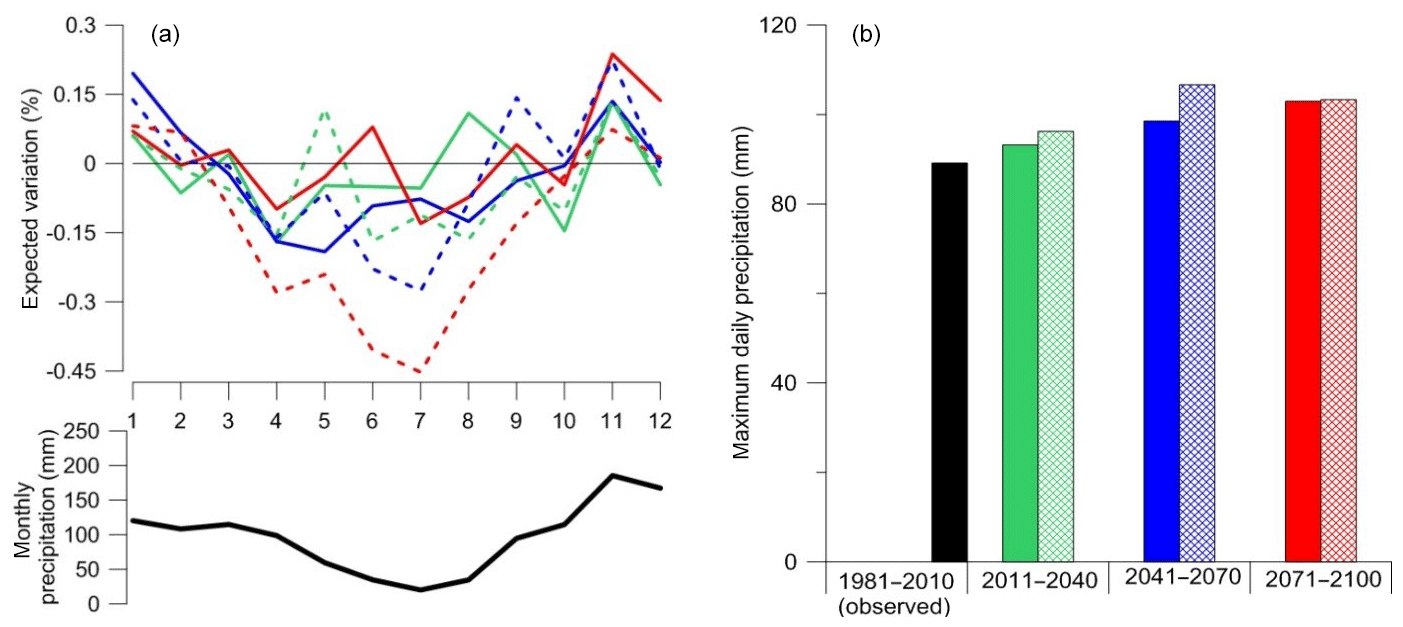
Figure 5(a) expected variations in monthly cumulative variations and (b) mean values of maximum daily precipitation.
In this study, cumulative rainfall parameters were calculated using a moving window procedure associated with each day from 1 January 1960 to 31 December 2015 from the observed precipitation data described in Sect. 4.1. The number of events observed for each day at the Nocera Inferiore, Gragnano and Castellammare di Stabia, as reported in the inventory, were associated with the rainfall data. Figure 6 plots the pairs of β01 and β59 recorded daily in the period 1960–2015, along with the indication of the occurrence (by site) or non-occurrence of flow-like landslide events.
The probability of event occurrence is given by
where is the ith value of cumulative rainfall β01 (i=1, …, , is the jth value of cumulative rainfall β59 (j=1,…, , and is the conditional probability of triggering of a flow-like landslide given the simultaneous occurrence of and .
The joint probability of the simultaneous occurrence of and is obtained as the frequentist ratio of the number of days in which the simultaneous occurrence of and was recorded to the total number of days for which observations at the rain gauges are available. While is assumed to be temporally variable due to the climate-change-induced variations in rainfall patterns over time, the triggering probability is assumed to be an inherent, temporally invariant characteristic of the study area, as it parameterizes, in terms of probability, the susceptibility of the triggering of flow movements in the area in response to the attainment of specific rainfall thresholds. It accounts implicitly and empirically for all physical factors affecting triggering mechanisms. The triggering probability is calculated as described in the following section.
5.2 Triggering probability calculation method
The conditional probability of the triggering of a flow-like landslide given the simultaneous occurrence of and is estimated using a Bayesian approach as suggested by Berti et al. (2012). The procedure refers to Bayes' theorem, formulated as follows:
where, in the Bayesian glossary, is the likelihood, i.e., the conditional joint probability of the simultaneous occurrence of and if an event is triggered in the reference area, and P(T) is the prior probability, i.e., the probability of triggering in the reference area, regardless of the magnitude of β01 and β59.
Let Nβ represent the total number of rainfall events recorded during a given reference time period, NL the total number of flow-like landslides occurred during the given reference time period, the number of rainfall events of a given magnitude of β01 recorded during the given time reference, and the number of rainfall events of a given magnitude of β59 recorded during the given time reference.
The likelihood can be calculated as the product of the marginal conditional probabilities of attainment of and given the occurrence
The above Bayesian probabilities can be computed in terms of relative frequencies as follows:
where is the number of rainfall events of a magnitude of at least recorded during the given time reference that resulted in the triggering of flow-like landslides, and is the number of rainfall events of a magnitude of at least recorded during the given time reference that resulted in the triggering of flow-like landslides.
Figure 7 plots triggering probability PT as a function of 1-day and 59-day cumulative rainfall, as estimated through the Bayesian approach. Possible future variations in land use and land cover features are assumed not to significantly affect proxy values. This is a simplistic hypothesis, as local conditions could substantially modify the susceptibility of the areas to event occurrence (e.g., fires destroying vegetation). Should substantial variations in physical factors occur in the study area, a re-evaluation of triggering probability is warranted.
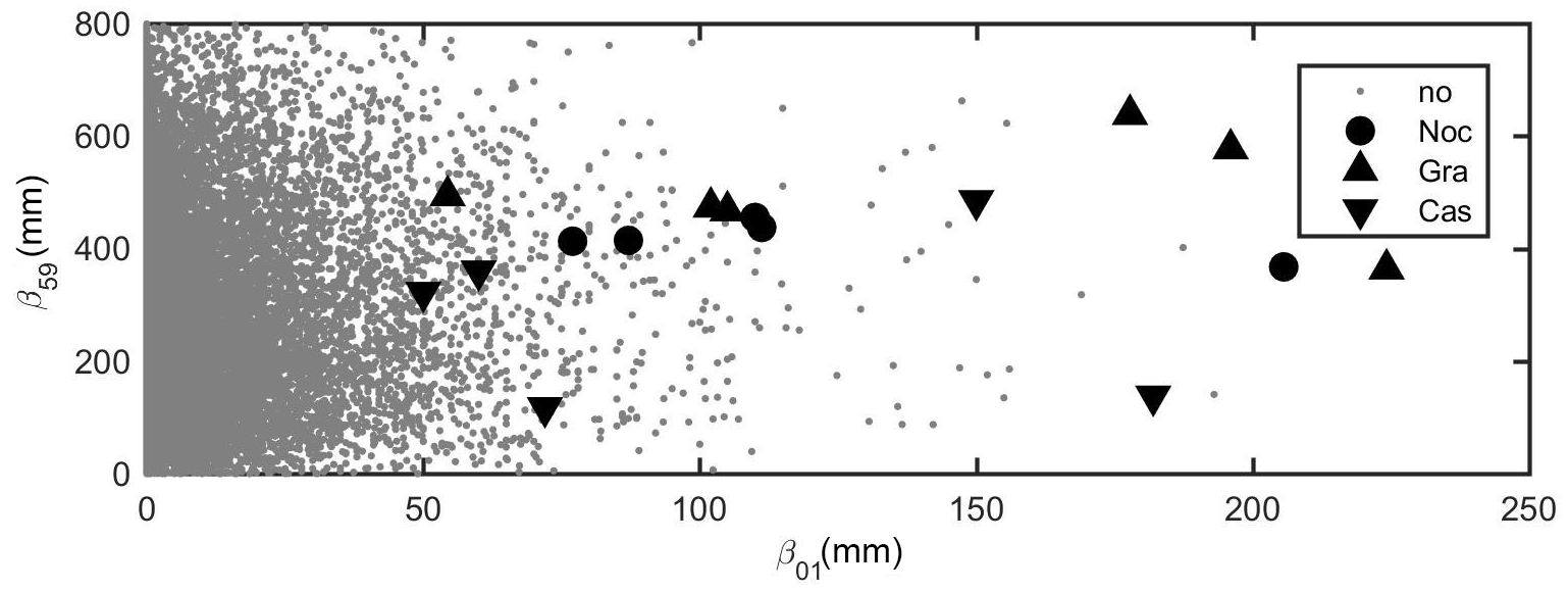
Figure 6Pairs of cumulative rainfall thresholds β01 and β59 recorded daily in the period 1960–2015, with occurrence (by site) or non-occurrence of landslide events.
5.3 Occurrence probability outputs
Following the quantitative estimation of the site-specific triggering probability as described above, flow-slide occurrence probability was calculated using Eq. (2) for each of the 10 EURO-CORDEX ensemble models and for 10 sets of 30-year intervals from 1981–2010 to 2071–2100 for both the RCP4.5 and RCP 8.5 scenarios.
A quantitative statistical analysis was conducted with the aim of analyzing ensemble outputs. The first module of the analysis consisted of the second-moment statistical characterization of the output samples. Such characterization involved the calculation of the mean, standard deviation, and sample coefficient of variation (given by the ratio of the latter to the former) for the 10-valued sets of ensemble model outputs for each of the 10 30-year intervals. Figure 8 plots the temporal variation of PL for 10 sets of 30-year intervals from 1981–2010 to 2071–2100 and for the RCP4.5 and RCP 8.5 scenarios, more specifically, model outputs and ensemble means for RCP4.5 (8a), RCP8.5 (8b), and for both concentration scenarios (8c). Figure 8d plots the sample coefficient of variation for both scenarios.
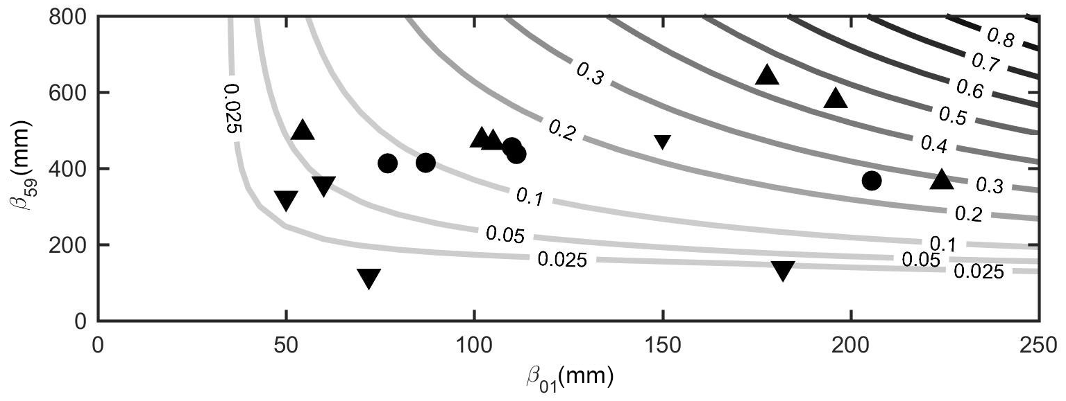
Figure 7Landslide triggering probability PL as a function of 1-day and 59-day cumulative rainfall.
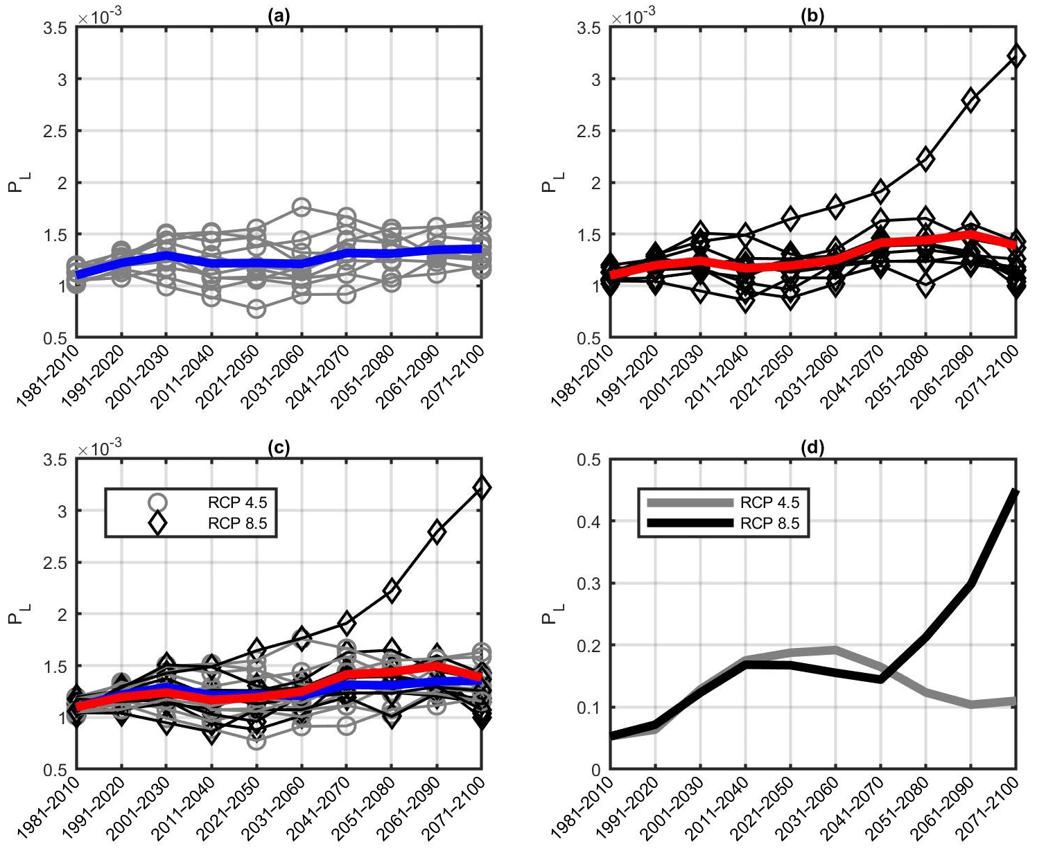
Figure 8Outputs of the second-moment statistical analysis of landslide occurrence probability PL.
For the RCP4.5 scenario, considering the running 30-year averages, a visual inspection of Fig. 8 suggested that all available projections predict a moderate increase in occurrence probability. A higher spread among the models is recognizable at the middle of the twenty-first century, as parameterized by the peak in the sample coefficient of variation. Such an increased spread is mainly due to the outputs of two models constantly representing the upper and bottom boundaries of the ensemble throughout the entire period investigated. For the RCP8.5 scenario, one of the 10 ensemble models yields occurrence probability values that progressively increase with respect to the other models over time. This leads to a marked increase in the scatter as parameterized by the sample coefficient of variation.
The second module of the statistical analysis consisted of the assessment of the existence and strength of a temporal statistical trend in occurrence probability values for the comprehensive set of output of the 10 models in the CORDEX ensemble for the 10 sets of 30-year periods. This analysis was conducted by means of two non-parametric statistical tests aimed at assessing the statistical independence between occurrence probability and time (as parameterized by a 30-year interval to which a specific occurrence probability value pertains) through the calculation of rank correlation statistics and related p values that parameterize the significance level at which the null hypothesis of statistical independence can be accepted. Spearman's test (Spearman, 1904) entails the calculation of Spearman's rank correlation coefficient ρ, which measures rank correlation on a scale (−1 is the full negative rank correlation, 0 is no rank correlation, and 1 is the full rank correlation) for an associated p value. The output values of ρ were 0.351 for RCP4.5 and 0.381 for RCP8.5. The associated p values were calculated as for RCP4.5 and for RCP8.5, attesting to a very low significance level for the rejection of the null hypothesis of statistical independence between the time and occurrence probability. Kendall's test (Kendall, 1938) entails the calculation of the statistic τ, which measures rank correlation on a scale (−1 is the full negative rank correlation, 0 is no rank correlation, 1 is the full rank correlation) for an associated p value. The output values of τ were 0.245 for RCP4.5 and 0.277 for RCP8.5. The associated p values were calculated as for RCP4.5 and for RCP8.5, again attesting to a very low significance level for the rejection of the null hypothesis. The non-parametric analysis thus assessed the existence of a strong statistical dependency of occurrence probability from time, thereby confirming the influence of climate change on flow-like movement hazard.
The third module consisted of the concise formulation of occurrence probability through the fitting of analytical models. The purpose of this model was to allow for a more concise forward estimation of triggering probability. In this study, the fitting of analytical models was conducted with the aim of relating analytically calculated values to specific levels of the likelihood of exceeding the occurrence probability. This was achieved through quantile regression.
Quantile regression is a type of regression analysis often used in statistics and econometrics. Whereas the method of least squares results in estimates that approximate the conditional mean of the response variable given certain values of the predictor variables, quantile regression aims at estimating any user-defined quantile of a response variable in this case of triggering probability (Yu et al., 2003). Quantile regression implements a minimization algorithm and yields model parameters that define the analytical model for user-defined regression quantiles (corresponding to a likelihood of non-exceedance). The use of quantile regression enables us to address explicitly different levels of conservatism in the output models, with higher quantiles corresponding to higher levels of conservatism. Quantiles of 0.50 and 0.90 were considered, corresponding to 50 % and 10 % likelihoods of exceedance, i.e., to scenarios of medium and high conservatism, respectively.
In applying quantile regression, a variety of analytical models were adapted to the dataset, including the linear, power, logarithmic, and modified geometric models. Among those, the third displayed the best goodness of fit. The modified geometric model employed in this study is given by
where p1 and p2 are the model parameters to be estimated using quantile regression and t30=1 … 10 is an auxiliary discrete natural variable referring to the ordinality of the 30-year averaging interval (e.g., 1981–2010 is interval “1” and 2071–2100 is interval “10”). Fig. 9a and b show the quantile regression-based fits of the modified geometric model to the samples of occurrence probability values for likelihoods of exceedance of 50 % (Q50) and 10 % (Q90) for RCP4.5 and RCP8.5, respectively.
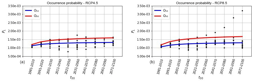
Figure 9Fitting of modified geometrical models to landslide occurrence probability ensemble data for quantiles Q50 and Q90: (a) RCP4.5 and (b) RCP8.5.
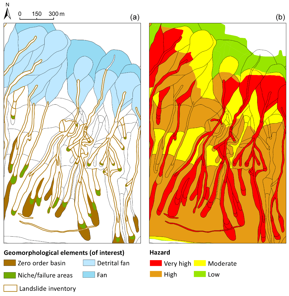
Figure 10Geomorphological (a) and hazard maps (b) of the Landslide Risk Management Plan of the River Basin Authority (PSAI; in Italian, Piano Stralcio di Assetto Idrogeologico, 2015).
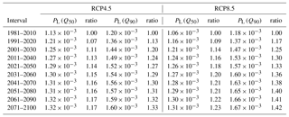
The output model parameters for RCP4.5 were and for Q50 and and for Q90. For RCP8.5, and for Q50 and and for Q90. While the plots show a continuous fitted model for the sake of visual appreciation of the quantile regression outputs, it must be noted that t30 is a discrete variable that can only take integer values between 1 and 10. Table 4 illustrates the values of occurrence probability as calculated from the modified geometric models for Q50 and Q90. The ratios of occurrence probability of a given interval to those of the observed data (1981–2010) are also provided to provide a quantitative measure of the effect of climate change over time. The findings displayed comparable increases under both RCPs, with no clear increases for the more severe scenario. Such results are consistent with variations shown in Fig. 4, where monthly anomalies and future expected values in maximum daily precipitation are reported. While decreases during the dry season are clearly more remarkable under RCP8.5, increases during the fall and winter seasons do not return clear patterns regulated by scenarios or time horizons. In this perspective, no significant differences between RCPs are observed.
Table 4Temporal evolution of occurrence probability for RCP4.5 and RCP8.5 (50th and 90th quantiles).
It is worth recalling that the present approach neglects several dynamics (e.g., effects of evapotranspiration reducing the soil moisture), which could play a significant role because of increased warming. For any given time interval and level of conservatism, occurrence probability is assumed to be spatially uniform within the study area, since the database that is used to develop the Bayesian method refers to the entire area itself. As detailed in a similar study by Berti et al. (2012), the quantitative output of empirical methods such as the one developed in the paper implicitly accounts for the spatial variability (if any) of rainfall characteristics within the area. In this study, three distinct reference weather stations were used for the three towns. The analysis of Nocera relies only on the local weather station, whose data were also used for bias correction purposes. Given the limited geographical extension of the area, the component of epistemic uncertainty due to spatial variability is not expected to be significant.
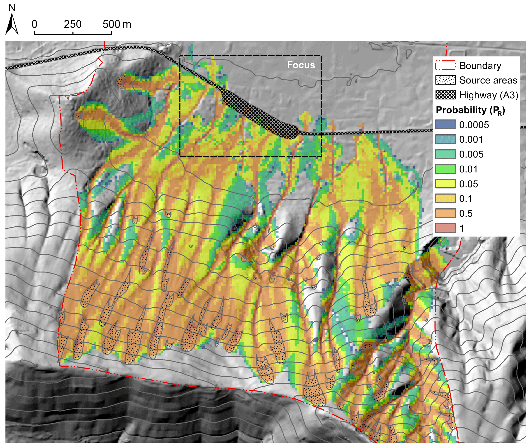
Figure 11Spatial distribution of reach probability at hillslope scale; the area corresponds to the box named “Mt. Albino” in Fig. 2.
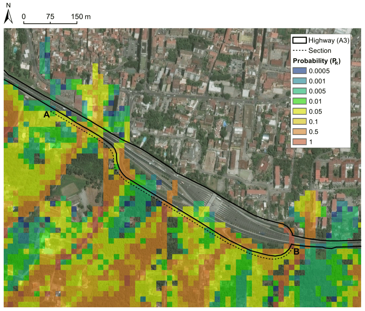
Figure 12Spatial distribution of reach probability at infrastructure scale and indication of section A–B.
Investigation of the spatial variability of flow-like landslide hazard entails the modeling of its downslope propagation (runout). Reach probability is the probability (from 0, certainty of no reach, to 1, certainty of reach) of each point in the spatial domain being affected by the event during the runout process. Several morphologically, empirically, and physically based approaches are available for quantitative runout analysis (Hürlimann et al., 2008). Each of these may present advantages or weaknesses in relation to site- and/or phenomenon-specific attributes, data availability, and the scale of the analysis. Consistent with the methods previously used to define rainfall-triggering scenarios, the approach used to define downslope runout scenarios is based on an algorithm involving stochastic modeling.
6.1 Reach probability calculation method
Reach probability was computed spatially using Flow-R, a DTM-based distributed empirical model developed in the Matlab® environment (Horton et al., 2013). Due to the large geographical scale of the area and to the deep complexity of the analyzed phenomena, an approach that was not highly parameter-dependent was deliberately adopted. A variety of DTM resolutions were tested for the case study, and a 15×15 m resolution was chosen. Comparing the DTM with the real current morphological shape of the areas both numerically and by expert judgment, the adopted resolution is deemed to represent the channelized shape and the fan areas with good accuracy, confirming the Horton et al. (2013) observations. The flow-slide spreading is controlled by a flow direction algorithm that reproduces flow paths (Holmgren, 1994) and by a persistence function to consider inertia and abruptness in change of the flow direction (Gamma, 2000). In the setting used in this study (x=1, see Eq., 3 in Horton et al., 2013), the flow direction algorithm proposed by Holmgren (1994) is similar to the multiple D8 of Quinn et al. (1991, 1995). The multiple D8 distributes the flow to all neighboring downslope cells weighted according to slope. The algorithm tends to produce more realistic-looking spatial patterns than the simple D8 algorithm by avoiding concentration in distinct lines (Seibert and McGlynn, 2007). The maximum possible runout distances are computed by means a simplified friction-limited model based on a unitary energy balance (Horton et al., 2013).
One-run propagation simulation provides possible flow-paths generated from previously identified triggering or source areas. In this work, source areas were identified by means of the official geomorphological map of the “Campania Centrale” River Basin Authority (PSAI, 2015). The set of source areas coincides with the union of the “zero order basin” (ZOB) and current “niche/failure” areas, as shown in Fig. 10. This hypothesis is in accordance with the requirement of consistency with accounts of historical events and with the aim of considering the most pessimistic possible triggering scenarios (i.e., those with maximum mass potential energy).
The reach probability for any given cell PR is calculated by the following equation:
where u and v are the flow directions, pu is the probability value in the uth direction, is the flow proportion according to the flow direction algorithm, is the flow proportion according to the persistence function, and p0 is the probability determined in the previous cell along the generic computed path. The values are subsequently normalized. Runout routing is stopped when (1) the angle of the line connecting the source area to the most distant point reached by the flow slide along the generic computed path is smaller than a predefined angle of reach (Corominas, 1996) and (2) the velocity exceeds a user-fixed maximum value or is below the value corresponding to the maximum energy lost due to friction along the path. The values that do not fit the aforementioned requirements are redistributed among the active cells to ensure the conservation of the total probability value.
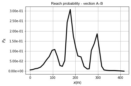
Figure 13Reach probability along the A–B section (Fig. 12) of the A3 motorway (point A is located at x=0).
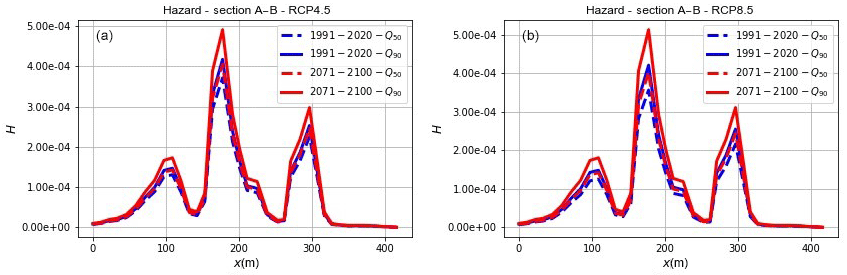
Figure 14Landslide hazard for section A–B, calculated for time intervals 1991–2020 and 2071–2100 and for quantiles Q50 and Q90: (a) RCP4.5 and (b) RCP8.5.
6.2 Reach probability outputs
The propagation routine was applied to the DTM described in Sect. 3. An angle of reach of 4∘ was calibrated based on the geomorphological information (i.e., the extension of the slope fan deposition) and the official hazard maps of the Landslide Risk Management Plan of the River Basin Authority (PSAI, 2015) shown in Fig. 10, considering a “paroxysmal” event. Consistent with the mean values reported by the scientific literature (Faella and Nigro, 2001; Revellino et al., 2004) for the same phenomena and in the same region, the maximum runout velocity was set at 10 m s−1. Figure 11 illustrates the spatial distribution of reach probability at the hillslope scale. Source areas are also indicated. The runout characteristics of the event types considered (types “b” and “c”; see Sect. 2.1) can be significantly different. Nevertheless, the same set of parameters (reach angle and velocity) satisfies both event conditions adequately. It may be noted that one un-channelized event (March 2005) was considered in this study.
In this area, the highway runs mostly on a soil embankment. The road level is generally elevated with respect to the paths of the downslope flows. The propagation impacts the embankment and stops in front of – or laterally continues according to – the topographic information and the model setting. Differently, in some points, the highway runs approximately at the same level of the fans, thereby allowing the propagating flow to run onto the road. In both cases, damage or disruptions may be caused to the infrastructure. In order to overcome this distinction and to cover both scenarios, only flow propagation to the upstream boundary of the infrastructure is considered in the study. An illustrative example is shown in the magnified focus area in Fig. 12. Due to the reasons mentioned above, the road's surface is only partially affected by the flow slides. This study focuses on a 400 m stretch of the infrastructure (from point A to point B in Fig. 12), the runout values to be considered in the risk assessment should be taken along the section A–B (Fig. 12). The results shown in Fig. 13 attest to the marked spatial variability of reach probability along the investigated section of the A3 motorway infrastructure.
Once occurrence probability and reach probability have been estimated as illustrated in Sects. 5 and 6, respectively, it is possible to calculate hazard using Eq. (1). Hazard is temporally variable, because occurrence probability displays temporal variability as a consequence of climate change, as shown in Sect. 5.3. Reach probability is assumed to be temporally invariant, as it is deterministically related to terrain morphology. This entails that the reach probability outputs obtained in Sect. 6.2 are valid only for the current terrain morphology. Should significant variations in terrain morphology occur, for instance, in case of the occurrence of flow-like landslides, reach probability would need to be reassessed, as described in Sect. 6.1.
To complete the flowchart shown in Fig. 4, an example calculation of hazard is provided for the section A–B. Figure 14 shows the spatially and temporally variable hazard profile for time intervals 1991–2020 and 2071–2100, for both quantiles Q50 and Q90 and for RCP4.5 and RCP 8.5. The occurrence probability values used to multiply the reach probability values shown in Fig. 13 are taken from Table 4. Thus, the estimated variations primarily reflect changes in occurrence probability due to expected climate change. In this regard, an increase is estimated under both concentration scenarios, Trends in the increase are related to the severity of scenario (the more severe, the higher the increase) and the investigated percentile (the less frequent, the higher the increase). In spatial terms, more pronounced increases in hazard are detectable in the current peak reach probability, which increases from to .
This paper has illustrated an innovative methodology for the quantitative estimation of rainfall-induced flow-like movement hazard. An example of the application of the proposed method was conducted for a short section of a motorway. The quantitative approach to hazard estimation was pursued through the implementation of models that are capable of simulating both deposition and entrainment, similar to other notable literature contributions (e.g., Deangeli, 2008; Rosatti and Begnudelli, 2013; Frank et al., 2015; Stancanelli et al., 2015; Cuomo et al., 2016; Gregoretti et al., 2018). Despite the limited extension of the study area, the results displayed a marked temporal and spatial variability of hazard. The temporal variability of hazard is a consequence of climate change as parameterized through quantitative projections for concentration scenarios RCP4.5 and RCP8.5. Significant temporal variability was assessed for both concentration scenarios. The considerable spatial variability resulting from the case study stems from the spatial variability of reach probability, as modeled in the runout analysis.
The calculation of occurrence probability, specifically in the triggering probability calculation phase, relies on a Bayesian approach that replicates the one provided by Berti et al. (2012). This study replicates the hypotheses and glossary introduced by these researchers and shares the implications and possible limitations of such an approach. For instance, the modeling hypothesis by Berti et al. (2012) is adopted, in which multiple flow-like landslides are counted as one single event. Hence, the Bayesian method presented in the paper quantifies the probability of occurrence of a landslide scenario (defined as “at least one event in the proximity area”) in a well-defined time period (30 years). This definition of scenario is semantically consistent with the one provided by Corominas et al. (2015) Reach probability, as estimated quantitatively in the study, is consistent with this definition, as it is calculated from the superposition of all possible runout paths from all events potentially occurring from all source areas. Hazard, as calculated using the above hypotheses, is thus a conservative, upper-bound estimate related to a specific rainfall scenario involving specific values of 1-day and 59-day cumulative rainfall. From a semantic standpoint, hazard as defined herein is also consistent with the reference glossary provided by Corominas et al. (2015).
The quantitative estimates of hazard as obtained in this paper are pervaded by significant uncertainty. Among the main sources of uncertainty are the climate change projections, the runout model, and the Bayesian model developed to quantify triggering probability. These uncertainties are epistemic in nature, as they stem from the inherent difficulty in compiling climate change projections, the inevitable degree of approximation and imperfection in runout modeling capabilities, and the limited rainfall and flow-like landslide occurrence data used to develop triggering probability curves. As such, increased modeling capability and improved databases could reduce the magnitude of uncertainty associated with hazard estimation.
The hazard outputs obtained by the method can be used directly in the quantitative estimation of risk. The latter also requires the quantitative estimation of the vulnerability of human-valued assets (i.e., vehicles, persons, etc.) and the exposure (i.e., the number and/or degree of presence) of the assets themselves in the study area in a referenced time period.
Notwithstanding the above uncertainties and limitations, the quantitative estimation and assessment of the spatial and temporal variability of hazard provide an important decision support tool in the disaster risk management cycle, specifically in the planning and prioritization of hazard mitigation and risk mitigation measures. The availability of quantitative methods allows for a more rational decision-making process in which the costs and effectiveness of risk mitigation can be compared and assessed.
Campanian pyroclastic covers are characterized by several specific features (high porosity, significant water retention capacity, and intermediate saturated hydraulic conductivities) playing a relevant role for triggering (e.g., role of antecedent precipitation or the persistency and/or magnitude of a potential triggering event). Moreover, stratigraphic details like the actual grain size distribution, the presence of pumice lenses, or the depth of pyroclastic deposits regulated by the distance from the eruptive centers and wind direction or magnitude during the eruptions also make generalizations within the same Campania region complex. Nevertheless, the framework developed for the pyroclastic covers on the northern side of the Lattari Mountains (where Nocera Inferiore is located) appears easily transferable to other contexts where precipitation observations and details about the timing of flow-like movements are available. Similarly, the climate simulation chain follows the state-of-the-art analysis of impacts potentially induced by climate change. Finally, the estimated increases in hazard were consistent with the results reported in several works investigating the variation in frequency of events in coarse-grained soils (Gariano and Guzzetti, 2016).
EURO-CORDEX input data are freely available on the EURO-CODEX website platform. The data underlying the research are available on request by contacting corresponding author.
MU contributed the reference hazard framework (Sect. 3), the calculation of occurrence and triggering probabilities (Sect. 5), and the calculation of hazard (Sect. 7). GR and FC provided the background about the investigated landslide dynamics and contributed the description and modelling of the study area (Sect. 2); GR and PM performed data stocktaking for the reference rainfall and landslide inventory datasets and carried out the proper analysis of climate projections (Sect. 4). GR wrote the Introduction (Sect. 1). FC contributed the calculation of reach probability (Sect. 6). UKE contributed to the definition of the general hazard framework (Sect. 3) and to the calculation of occurrence and triggering probabilities (Sect. 5). All authors contributed jointly to the definition of the general layout of the paper and the concluding remarks (Sect. 8).
The authors declare that they have no conflict of interest.
This article is part of the special issue “Landslide early warning systems: monitoring systems, rainfall thresholds, warning models, performance evaluation and risk perception”. It is not associated with a conference.
The research leading to these results has received funding from the European
Union Seventh Framework Program (FP7/2007-2013) under grant agreement
no. 606799. The support is gratefully acknowledged.
Edited by: Paolo Tarolli
Reviewed by: three
anonymous referees
Berti, M., Martina, M. L. V., Franceschini, S., Pignone, S., Simoni, A., and Pizziolo, M.: Probabilistic rainfall thresholds for landslide occurrence using a Bayesian approach, J. Geophys. Res., 117, F04006, https://doi.org/10.1029/2012JF002367, 2012.
Beven, K. J.: EGU Leonardo Lecture: facets of hydrology – epistemic error, non- stationarity, likelihood, hypothesis testing, and communication, Hydrolog. Sci. J., 61, 1652–1665, https://doi.org/10.1080/02626667.2015.1031761, 2015.
Beven, K. J., Aspinall, W. P., Bates, P. D., Borgomeo, E., Goda, K., Hall, J. W., Page, T., Phillips, J. C., Simpson, M., Smith, P. J., Wagener, T., and Watson, M.: Epistemic uncertainties and natural hazard risk assessment – Part 2: What should constitute good practice?, Nat. Hazards Earth Syst. Sci., 18, 2769–2783, https://doi.org/10.5194/nhess-18-2769-2018, 2018.
Cascini, L., Cuomo, S., and Guida, D.: Typical source areas of May 1998 flow-like mass movements in the Campania region, Southern Italy, Eng. Geol., 96, 107–125, 2008.
Chancel, L. and Piketty, T.: Carbon and inequality: from Kyoto to Paris. Trends in the global inequality of carbon emissions (1998–2013) & prospects for an equitable adaptation fund, Iddri & Paris School of Economics Report, 2015.
Ciervo, F., Rianna, G., Mercogliano, P., and Papa, M. N.: Effects of climate change on shallow landslides in a small coastal catchment in southern Italy, Landslides, 14, 1043–1055, https://doi.org/10.1007/s10346-016-0743-1, 2016.
Comegna, L., De Falco, M., Jalayer, F., Picarelli, L., and Santo, A.: The role of the precipitation history on landslide triggering in unsaturated pyroclastic soils in Advancing Culture in living with landslides, edited by: Mikoš, M., Casagli, N., Yin, Y., and Sassa, K., Springer International Publishing 2017, https://doi.org/10.1007/978-3-319-53485-5_3, 2017.
Cooke, R. M.: Messaging climate change uncertainty, Nat. Clim. Change, 5, 8–10, https://doi.org/10.1038/nclimate2466, 2014.
Copons, R. and Vilaplana, J. M.: Rockfall susceptibility zoning at a large scale: From geomorphological inventory to preliminary land use planning, Eng. Geol., 102, 142–151, 2008.
Corominas, J.: The angle of reach as a mobility index for small and large landslides, Can. Geotech. J., 33, 260–271, https://doi.org/10.1139/t96-130, 1996.
Corominas, J., Einstein, H., Davis, T., Strom, A., Zuccaro, G., Nadim, F., and Verdel, T.: Glossary of Terms on Landslide Hazard and Risk, in: Engineering geology for society and territory – Volume 2: Landslide processes, edited by: Lollino, G., Giordan, D., Crosta, G. B., Corominas, J., Azzam, R., Wasowski, J., and Sciarra, N., Springer International Publishing Switzerland, 1775–1779, https://doi.org/10.1007/978-3-319-09057-3_314, 2015.
Costa, J. E.: Physical geomorphology of debris flows, in: Developments and Applications of Geomorphology, edited by: Costa, J. E. and Fleisher, P. J., Berlin, Springer-Verlag, 268–317, 1984.
Cox, L. A.: Confronting deep uncertainties in risk analysis, Risk Anal., 32, 1607–1629, 2012.
Cuomo, S., Pastor, M., Capobianco, V., and Cascini, L.: Modelling the space- time bed entrainment for flow-like landslide, Eng. Geol., 212, 10–20, https://doi.org/10.1016/j.enggeo.2016.07.011, 2016.
Damiano, E. and Mercogliano, P.: Potential effects of climate change on slope stability in unsaturated pyroclastic soils, in: Book Series “Landslide Science and Practice”, Vol. 4 “Global Environmental Change”, edited by: Margottini, C., Canuti, P., and Sassa, K., 4, 15–25, 2013.
Deangeli, C.: Laboratory granular flows generated by slope failures, Rock Mech. Rock Eng., 41, 199–217, 2008.
De Vita, P. and Piscopo, V.: Influences of hydrological and hydrogeological conditions on debris flows in peri-vesuvian hillslopes, Nat. Hazards Earth Syst. Sci., 2, 27–35, https://doi.org/10.5194/nhess-2-27-2002, 2002.
Dietrich, W. E., Wilson, C. J., and Reneau, S. L.: Hollows, colluvium, and landslides in soil-mantled landscapes, Hillslope Processes, edited by: Abrahams, A. D., Allen and Unwin, Boston, Mass., 361–388, 1986.
Ehret, U., Zehe, E., Wulfmeyer, V., Warrach-Sagi, K., and Liebert, J.: HESS Opinions “Should we apply bias correction to global and regional climate model data?”, Hydrol. Earth Syst. Sci., 16, 3391–3404, https://doi.org/10.5194/hess-16-3391-2012, 2012.
Faella, C. and Nigro, E.: Effetti delle colate rapide sulle costruzioni. Parte Seconda: Valutazione della velocita` di impatto, Forum per il Rischio Idrogeologico “Fenomeni di colata rapida di fango nel Maggio '98”, Napoli, 22 giugno 2001, 113–125, 2001.
Fell, R., Corominas, J., Bonnard, C., Cascini, L., Leroi, E., and Savage, W. Z.: Guidelines for landslide susceptibility, hazard and risk zoning for land-use planning (on behalf of the JTC-1 Joint Technical Committee on Landslides and Engineering Slopes), Eng. Geol., 102, 99–111, https://doi.org/10.1016/j.enggeo.2008.03.014, 2008.
Fiorillo, F. and Wilson, R. C.: Rainfall induced debris flows in pyroclastic deposits, Campania (southern Italy), Eng. Geol., 75, 263–289, 2004.
Frank, F., McArdell, B. W., Huggel, C., and Vieli, A.: The importance of entrainment and bulking on debris flow runout modeling: examples from the Swiss Alps, Nat. Hazards Earth Syst. Sci., 15, 2569–2583, https://doi.org/10.5194/nhess-15-2569-2015, 2015.
Gamma, P.: Ein Murgang-Simulationsprogramm zur Gefahrenzonierung, Geographisches Institut der Universität Bern, 2000.
Gariano, S. L. and Guzzetti, F.: Landslides in a changing climate, Earth-Sci. Rev., 162, 227–252, https://doi.org/10.1016/j.earscirev.2016.08.011, 2016.
Giorgi, F. and Gutowski, W. J.: Coordinated Experiments for Projections of Regional Climate Change, Current Climate Change Reports, 2, 202–210, https://doi.org/10.1007/s40641-016-0046-6, 2016.
Gregoretti, C., Degetto, M., Bernard, M. and Boreggio, M.: The debris flow occurred at Ru Secco Creek, Venetian Dolomites, on 4 August 2015: analysis of the phenomenon, its characteristics and reproduction by models, Front. Earth Sci., https://doi.org/10.3389/feart.2018.00080, 2018.
Gudmundsson, L., Bremnes, J. B., Haugen, J. E., and Engen-Skaugen, T.: Technical Note: Downscaling RCM precipitation to the station scale using statistical transformations – a comparison of methods, Hydrol. Earth Syst. Sci., 16, 3383–3390, https://doi.org/10.5194/hess-16-3383-2012, 2012.
Hallegatte, S., Shah, A., Lempert, R., Brown, C., and Gill, S.: Investment decision making under deep uncertainty: application to climate change, Policy Research Working Paper 6193, 41, 2012.
Holmgren P.: Multiple flow direction algorithm for runoff modeling in grid-based elevation models: an empirical evaluation, Hydrol. Process., 8, 327–334, 1994.
Horton, P., Jaboyedoff, M., Rudaz, B., and Zimmermann, M.: Flow-R, a model for susceptibility mapping of debris flows and other gravitational hazards at a regional scale, Nat. Hazards Earth Syst. Sci., 13, 869–885, https://doi.org/10.5194/nhess-13-869-2013, 2013.
Hürlimann, M., Rickenmann, D., Medina, V., and Bateman, A.: Evaluation of approaches to calculate debris-flow parameters for hazard assessment, Eng. Geol., 102, 152–163, 2008.
Hutchinson, J. N.: Review of flow-like mass movements in granular and fine-grained materials, in: Proc. Int. Workshop Occurrence and Mechanisms of Flows in Natural Slopes and Earthfills, edited by: Picarelli, L., Patron, Bologna, Sorrento, 3–16, 2004.
Kendall, M.: A New Measure of Rank Correlation, Biometrika, 30, 81–89, https://doi.org/10.1093/biomet/30.1-2.81, 1938.
Koutsoyiannis, D. and Montanari, A.: Statistical analysis of hydroclimatic time series: Uncertainty and insights, Water Resour. Res., 43, W05429, https://doi.org/10.1029/2006WR005592, 2007.
Lafon, T., Dadson, S., Buys, G., and Prudhomme, C.: Bias correction of daily precipitation simulated by a regional climate model: a comparison of methods, Int. J. Climatol., 33, 1367–1381, 2013.
Maraun, D.: Bias correction, quantile mapping, and downscaling: revisiting the inflation issue, J. Climate, 26, 2137–2143, 2013.
Maraun, D. and Widmann, M.: The representation of location by a regional climate model in complex terrain, Hydrol. Earth Syst. Sci., 19, 3449–3456, https://doi.org/10.5194/hess-19-3449-2015, 2015.
Napolitano, E., Fusco, F., Baum, R. L., Godt, J. W., and De Vita, P.: Effect of antecedent-hydrological conditions on rainfall triggering of debris flows in ash-fall pyroclastic mantled slopes of Campania (southern Italy), Landslides, 13, 967–983, https://doi.org/10.1007/s10346-015-0647-5, 2016.
Nordhaus, W.: A Review of the “Stern Review on the Economics of Climate Change”, J. Econ. Lit., 45, 686–702, 2007.
Pagano, L., Picarelli, L., Rianna, G., and Urciuoli, G.: A simple numerical procedure for timely prediction of precipitation-induced landslides in unsaturated pyroclastic soils, Landslides 7, 273–89, 2010.
Pettitt, A.N.: A non-parametric approach to the change point problem, Appl. Stat., 28, 126–135, 1979.
Quinn, P. F., Beven, K. J., Chevallier, P., and Planchon, O.: The prediction of hillslope flowpaths for distributed modelling using digital terrain models, Hydrol. Process., 5, 59–80, 1991.
Quinn, P. F., Beven, K. J., and Lamb, R.: The ln(a/tanβ) index: How to calculate it and how to use it within the TOPMODEL framework, Hydrol. Process., 9, 161–182, 1995.
Reder, A., Rianna, G., Mercogliano, P., and Pagano, L.: Assessing the Potential Effects of Climate Changes on Landslide Phenomena Affecting Pyroclastic Covers in Nocera Area (Southern Italy), Procedia Earth Planet. Sci., 16, 166–176, https://doi.org/10.1016/j.proeps.2016.10.018, 2016.
Reder, A., Rianna, G., and Pagano, L.: Physically based approaches incorporating evaporation for early warning predictions of rainfall-induced landslides, Nat. Hazards Earth Syst. Sci., 18, 613–631, https://doi.org/10.5194/nhess-18-613-2018, 2018.
Revellino, P., Hungr, O., Guadagno, F. M., and Evans, S. G.: Velocity and runout simulation of destructive debris flows and debris avalanches in pyroclastic deposits, Campania region, Italy, Environ. Geol., 45, 295–311, https://doi.org/10.1007/s00254-003-0885-z, 2004.
Rianna, G., Pagano, L., and Urciuoli, G.: Rainfall Patterns Triggering Shallow Flowslides in Pyroclastic Soils, Eng. Geol., 174, 22–35, https://doi.org/10.1016/j.enggeo.2014.03.004, 2014.
Rianna, G., Comegna, L., Mercogliano, P., and Picarelli, L.: Potential effects of climate changes on soil–Atmosphere interaction and landslide hazard, Nat. Hazards, 84, 1487, https://doi.org/10.1007/s11069-016-2481-z, 2016.
Rianna, G., Reder, A., Mercogliano, P., and Pagano, L.: Evaluation of variations in frequency of landslide events affecting pyroclastic covers in the Campania region under the effect of climate changes, Hydrology, 4, 34, https://doi.org/10.3390/hydrology4030034, 2017a.
Rianna, G., Reder, A., Villani, V., and Mercogliano, P.: Variations in Landslide Frequency Due to Climate Changes Through High Resolution Euro-CORDEX Ensemble, in: Advancing Culture of Living with Landslides, edited by: edited by: Mikoš, M., Casagli, N., Yin, Y., and Sassa, K., WLF 2017, Springer, Cham, https://doi.org/10.1007/978-3-319-53485-5_27, 2017b.
Rosatti, G. and Begnudelli, L.: Two dimensional simulations of debris flows over mobile beds: enhancing the TRENT2D model by using a well-balanced generalized Roe-type solver, Computational Fluids, 71, 179–185, https://doi.org/10.1016/j.compfluid.2012.10.006, 2013.
Rouiller, J. D., Jaboyedoff, M., Marro, C., Philippossian, F., and Mamin, M.: Pentes instables dans le Pennique valaisan, vdf Hochschulverlag AG and ETH, Zurich., Rapport final du Programme National de Recherche PNR 31/CREALP, 98, 239 pp., 1998 (in French).
Seibert, J. and McGlynn, B. L.: A new triangular multiple flow direction algorithm for computing upslope areas from gridded digital elevation models, Water Resour. Res., 43, W04501, https://doi.org/10.1029/2006WR005128, 2007.
Seneviratne, S. I., Nicholls, N., Easterling, D., Goodess, C. M., Kanae, S., Kossin, J., Luo, Y., Marengo, J., McInnes, K., Rahimi, M., Reichstein, M., Sorteberg, A., Vera, C., and Zhang, X.: Changes in climate extremes and their impacts on the natural physical environment, in: Managing the Risks of Extreme Events and Disasters to Advance Climate Change Adaptation, edited by: Field, C. B., Barros, V., Stocker, T. F., Qin, D., Dokken, D. J., Ebi, K. L., Mastrandrea, M. D., Mach, K. J., Plattner, G.-K., Allen, S. K., Tignor, M., and Midgley ,P. M., A Special Report of Working Groups I and II of the Intergovernmental Panel on Climate Change (IPCC), Cambridge University Press, Cambridge, UK, and New York, NY, USA, 109–230, 2012.
Smadi, M. M. and Zghoul, A.: A sudden change in rainfall characteristics in Amman, Jordan during the mid-1950s, American Journal of Environmental Sciences, 2, 84–91, 2006.
Spearman, C.: The proof and measurement of association between two things, Am. J. Psychol., 15, 72–101, https://doi.org/10.2307/1412159, 1904.
Stancanelli, L. M. and Foti, E.: A comparative assessment of two different debris flow propagation approaches – blind simulations on a real debris flow event, Nat. Hazards Earth Syst. Sci., 15, 735–746, https://doi.org/10.5194/nhess-15-735-2015, 2015.
Stein, S. and Stein, J. L.: Shallow Versus Deep Uncertainties in Natural Hazard Assessments, EOS T. Am. Geophys. Un., 94, 133–134, https://doi.org/10.1002/2013EO140001, 2013.
Stern, N.: The Economics of Climate Change: The Stern Review. Cambridge and New York, Cambridge University Press, ISBN: 0-521-70080-9, 2007.
United Nations: Framework Convention on Climate Change, Adoption of the Paris Agreement, 21st Conference of the Parties, Paris, United Nations, 2015.
Vallario, A.: Il dissesto idrogeologico in Campania, CUEN, ISBN: 9788871465661, 2000.
Villani, V., Rianna, G., Mercogliano, P., and Zollo, A. L.: Statistical approaches versus weather generator to downscale RCM outputs to slope scale for stability assessment: a comparison of performances, Electronic Journal of Geotechnical Engineering, 20, 1495–1515, 2015.
Wilby, R. L. and Dessai, S.: Robust Adaptation to Climate Change, Weather, 65, 176–80, 2010.
Yu, K., Lu, Z., and Stander, J.: Quantile regression: applications and current research areas, The Statistician, 52, 331–350, 2003.
- Abstract
- Introduction
- Description and modeling of the study area
- Hazard: glossary and model
- Source datasets
- Occurrence probability
- Reach probability
- Calculation of hazard
- Concluding remarks
- Data availability
- Author contributions
- Competing interests
- Special issue statement
- Acknowledgements
- References