Beyond and beneath displacement time series: towards InSAR-based early warnings and deformation analysis of the Achoma landslide, Peru

Detecting precursors to slope destabilisation with sufficient lead time and accuracy remains a challenging and unresolved issue in landslide hazard assessment and prediction. This is key, as catastrophic landslides often go unnoticed until immediately before or after failure, limiting opportunities for intervention. While in situ methods offer high accuracy at point locations, they are costly and require prior knowledge of instability. Satellite-based synthetic aperture radar differential interferometry (InSAR) has shown promise in identifying unknown landslides over large areas and has been proposed as a potentially useful tool for failure prediction. Typically valued for retrieving displacement time series, InSAR time series reliability depends heavily on successful interferogram unwrapping, which often leads to severe underestimations over landslides. Here, we analyse the deformation process of the Achoma landslide in Peru and demonstrate that the InSAR signal contains precursors based on alternative markers, even without displacement time series. Interferometric coherence shows the formation of gravitational structures up to 5 years before failure, as well as a critical shift in landslide behaviour 3 months prior to failure. Additionally, a marker based on the wrapped phase reveals and quantifies alternating periods of quiescence and motion, the latter becoming more frequent in the 2 years before failure. Our findings highlight the potential to use alternative InSAR signal markers to observe the deformation process and progressive failure leading up to the event, and to detect landslide precursors across extensive areas, providing valuable lead time for intervention and disaster prevention.

1 Introduction

Landslides pose a global threat, causing more than 4000 fatalities annually (Petley, 2012) including more than 4000 resulting from non-seismic triggers (Froude and Petley, 2018). Beyond the human toll, landslides lead to substantial social and economic consequences in both developing and developed countries. Despite advances in hazard assessment, predicting when and where potentially unstable hillslopes will fail catastrophically remains a major challenge. This highlights the critical importance of early identification of destabilizing slopes and the detection of accelerating phases, which are key to improving prediction and preparedness (e.g., Carlà et al., 2017; Roy et al., 2022; Strząbała et al., 2024; Valletta et al., 2022).

While there are documented instances of successful predictions and early warnings using in situ methods (e.g., Badoux et al., 2009; Fan et al., 2019; Loew et al., 2017), two main challenges persist: cost and feasibility of monitoring all known unstable slopes, and the limited pre-existing knowledge of instability, which often leads to landslides remaining unnoticed until severe acceleration or catastrophic failure occurs (Guzzetti, 2021; Palmer, 2017), causing significant delays in the installation of monitoring systems (e.g., Fiolleau et al., 2020).

The advent and use of satellite-based technologies, particularly satellite-based synthetic aperture radar differential interferometry (InSAR), have significantly improved landslide identification capabilities (e.g. Strząbała et al., 2024). Observations can be made more cost-effectively due to the increasing availability, frequency, and reliability of acquisitions, whilst the large coverage (Costantini et al., 2021, 2022; Wasowski and Bovenga, 2022) may allow for the identification of previously unknown unstable slopes at large scales (Dini et al., 2019, 2020). This enhances the possibility of implementing timely and targeted monitoring before disasters occur. Identifying destabilising slopes from satellite data is crucial also for landslides in remote locations, which are challenging to spot and monitor in situ, yet can generate far-reaching hazard cascades (Cook et al., 2021). With increasing temporal sampling of new generation satellites (e.g. Sentinel-1) and the potential for sub-centimetre displacement accuracy in favourable conditions (Ferretti et al., 2011; Liu et al., 2013; Wasowski and Bovenga, 2014), the use of InSAR has become widespread for generating landslide displacements time series based on small baseline subset (Berardino et al., 2002) (SBAS) or permanent scatterers (Ferretti et al., 2005, 2001) (PS) algorithms, and variations of these. In a few cases, retrospective retrieval of time series revealed acceleration patterns leading to failure, highlighting potential for accurate prediction of failure timing (Carlà et al., 2019; Intrieri et al., 2018).

However, despite InSAR's remarkable potential for geohazard observation, the universal reliability of InSAR displacement time series is not guaranteed, due to significant challenges related to the nature of the phenomena and data processing limitations. We highlight here only the limitations relevant to this work. For a more exhaustive account we refer to Lacroix et al. (2022a) and references therein.

Small to medium-size landslides (a few tens to a few hundred m along-scarp length) in many cases only cover a relatively small number of SAR pixels on the ground (e.g., for the pixel size of Sentinel-1, 2.3 m × 14.1 m), making signal detection challenging. Moreover, not all landslides are expected to exhibit measurable precursory deformation prior to failure. Rapid, shallow landslides in loose materials may fail abruptly with no significant precursors. Larger landslides (several hundred m along-scarp length) may exhibit displacements only on isolated sectors at different times. Additionally, landslides often present strong spatial gradients and sharp displacement edges (e.g. Cheaib et al., 2022) that make phase unwrapping problematic due to phase aliasing (Manconi, 2021; Strząbała et al., 2024). Finally, landslides often display non-linear behaviour in time, with phases of accelerations interspersed with periods of quiescence. This is unfavourable for InSAR time series based on SBAS or PS approaches (e.g. Handwerger et al., 2025), particularly when temporal sampling is affected by missing acquisitions or unusable images (e.g., snow cover, seasonal landcover changes). When a slope transitions from no displacement to fast reactivation, with displacements exceeding a threshold (commonly 1/4 of the wavelength) between two acquisitions and/or between adjacent pixels when gradients are strong, phase aliasing and decorrelation occur. The lack of phase continuity makes it difficult to accurately reconstruct the continuous phase signal from the wrapped phase measurements. As conventional processing methods for generating displacement time series rely on phase unwrapping, they are particularly susceptible to phase aliasing (Manconi, 2021). Moreover, as interferometric coherence decreases, unwrapping over critical areas might not be performed when processing large areas due to the cutoff imposed using coherence thresholds. This leads to the loss of any true deformation signal potentially contained in low- (or lower-) coherence interferograms. In essence, the success on landslide of common InSAR approaches heavily relies on the existence of many conditions favourable to processing. Without individual interferogram inspection, a time-consuming task, an InSAR displacement time series might seem accurate and plausible, yet it could significantly underestimate the true displacements and obscure crucial acceleration phases and/or their magnitude (Dini et al., 2020; Jacquemart and Tiampo, 2021). Consequently, there is a high potential for misinterpreting the ongoing processes driving instability and assessing the hazard level.

In response to the challenges associated with InSAR, some authors focused on the analysis of high temporal frequency optical images (e.g., Sentinel-2, PlanetLab) to derive time series of displacements (Lacroix et al., 2018, 2023), or changes in vegetation cover caused by landslides with NDVI from Sentinel-2 acquisitions (Yang et al., 2019). However, optical data are constrained by cloud coverage and have limited sensitivity to smaller displacements that might occur over longer time frames leading up to failure. Others have successfully retrieved acceleration phases through image correlation of SAR images (Li et al., 2020), but this method is also limited to the observation of relatively large displacements (greater than 1/10 of the pixel size), thus more suitable to cover the final weeks to months of an accelerating phase. Consequently, alternative and/or complementary InSAR-based techniques must be developed to improve our ability to observe landslide precursors beyond what is possible using only methods reliant on phase unwrapping. Jacquemart and Tiampo (2021) focused on InSAR coherence, showing a temporal decrease of coherence roughly 5 months prior to the Mudcreek landslide failure. To our knowledge this is the only study on this topic, highlighting the need for more case-studies and in-depth understanding of landslide behaviours associated with this type of signal. Since rapid, shallow landslides may fail without measurable precursors, coherence-based approaches are likely most effective for larger, slower, or more complex landslides where deformation evolves progressively over time.

Our work introduces a novel methodology for extracting landslide precursors that bypasses traditional time series generation. Instead, we integrate information on incipient and ongoing instability using interferometric coherence and wrapped phase. This approach is particularly valuable when full displacement time series are unavailable or unreliable. By addressing the limitations of conventional methods, we offer an alternative perspective on landslide precursor identification from space. This paper explores two critical questions: Can interferometric coherence serve as an effective precursor for identifying critical landslide phases and incipient instability in both time and space? And can indicators based on the wrapped phase provide insights into criticality of landslide behaviour, in the absence of a reliable displacement time series?

To illustrate our methodology, we present a case study on the Achoma landslide in the Colca Valley, Peru. This landslide exemplifies an instability that remained unnoticed on the ground until shortly before catastrophic failure, while retrospective analysis using optical satellite images detected signals 3 months before the event (Lacroix et al., 2023). Although our analysis is retrospective, the signals identified represent genuine precursory indicators detectable in the InSAR data before failure. Remarkably, our results show that signs of destabilisation were detectable 5 years prior to failure. The subsequent sections of this paper detail the methods we employed, including topographic error correction, coherence loss analysis, and the extraction of wrapped phase temporal behaviour. Finally, we present our results and discuss their significance, highlighting the potential integration of our approach with traditional methods.

2 Study area

The deeply incised Colca Valley is located in southern Peru. On its terraces, it hosts several settlements, largely supported by extensive agriculture. The valley is located between volcanic massifs to the north and south (Zerathe et al., 2016), and is characterised by sequences of ignimbrites and pyroclastic deposits. The valley's geomorphology has been shaped by debris avalanches from valley flank collapses followed by landslide dam breakouts (Thouret et al., 2007), with one such event forming a paleolake and depositing thick lacustrine deposits (Lacroix et al., 2015; Zerathe et al., 2016).

Seismicity in the region has distinct sources (Lacroix et al., 2023 and references therein; Zerathe et al., 2016), from relatively low magnitude (M_w < 3) seismic events originating in the volcanic area approximately 15–20 km to the southwest, to larger magnitude earthquakes associated with regional tectonic faults (M_w < 7) or M_w 8 events with origin in the subduction zone roughly 100 km to the west.

The area experiences a seasonal climate pattern, with most of the rainfall falling between December and April (Lacroix et al., 2015), followed by a dry season. Annual rainfall amounts range between 350 and 600 mm, with daily cumulative precipitation rarely exceeding 25 mm. Numerous large landslides dot the Colca valley (Pham et al., 2018), often showing retrogressive failure in the lacustrine deposits (Zerathe et al., 2016) and responding to different trigger mechanisms (Bontemps et al., 2020; Lacroix et al., 2015, 2023). Persistent uncertainties surround the factors controlling their evolution into slow or rapid landslides (Zerathe et al., 2016), making the evaluation of their hazard potential difficult. Other landslides in the valley that have been long creeping have been instrumented for years (Bontemps et al., 2020; Lacroix et al., 2014, 2015; Palmer, 2017), providing valuable insights into landslide dynamics and responses to seismic and climatic triggers.

The Achoma landslide, failed catastrophically on 18 June 2020, unnoticed for a long time until cracks were reported by locals in May 2020 (Dini et al., 2022; Lacroix et al., 2023), only 1 month prior to failure. It is a large and deep-seated landslide that spans approximately 800 m in width along its scarp and extends 500 m downslope to the Colca River, covering an area of about 0.4 km² (Fig. 1). The headscarp rises approximately 100 m high (Lacroix et al., 2023), with estimated rupture surface depth averaging 50 m. The landslide volume is thus estimated at around 20 × 10⁶ m³.

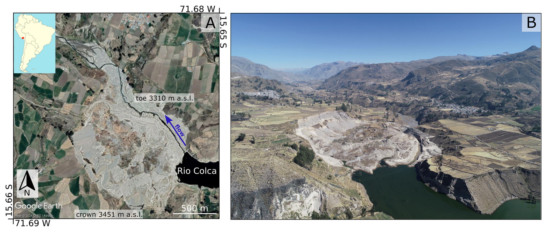
Figure 1 (A) Study area, Achoma landslide post failure (© GoogleEarth Image, CNES/Airbus 1 November 2020). Red rectangle in top left inset shows footprint of Sentinel 1 images (relative orbit number 47). (B) Drone image of the landslide, looking northwest. Credits: Ingemmet.

The failure occurred during the dry season, following cumulative rainfall of 600 mm during the preceding wet season. Earlier findings indicated the landslide gradually accelerated 3 months before its failure, initiating during the rainy season (Lacroix et al., 2023), suggesting rainfall may have played a crucial role in the transition from slow to rapid movement. The site has experienced seismic activity during the observation period, with the largest earthquake recorded on 15 August 2016, measuring M_w 5.5 (Bontemps et al., 2020).

3 Methods and data

3.1 Raw interferograms

We generated 514 Sentinel-1 wrapped interferograms (Dini et al., 2025b) from 114 satellite acquisitions of ascending track with relative orbit number 47, covering the period between 30 April 2015 and 20 June 2020 (the rupture of the Achoma landslide occurred on 18 June) over the Colca Valley, Peru. The interferograms were generated with the NSBAS processing chain (Doin et al., 2011), at medium spatial resolution. Sentinel-1 data, originally acquired with a ground resolution of 2.3 m in range and 14 m in azimuth, were multilooked (8 and 2 looks in range and azimuth, respectively) to a final pixel size of 18.4 m × 28.2 m. Temporal baselines range from 12 d (the minimum available for the area) to 1 year. The topographic contribution of the signal was removed with the SRTM 30 m digital elevation model. The interferograms were not filtered, in order to avoid possible artefacts and loss of deformation signal (Strozzi et al., 2020).

A first inspection of the interferograms was carried out, this revealed a non-linear behaviour of the landslide, characterised by phases of quiescence and activity. The nature of the landcover, largely composed of agricultural land and the intermittent, occasionally strong displacement gradients cause low coherence and low signal to noise ($S/N$) ratios in interferograms with temporal baselines of 48 d and longer. The highest signal-to-noise ($S/N$) ratios are observed for temporal baselines of 12 and 24 d. Thus, for the successive analyses described in the following sections, we selected a series of 113 successive interferograms with the shortest available baselines. Additionally, we included interferograms with baselines of 30, 48, and 72 d to cover periods where shorter baselines are unavailable due to missing images (Figs. S1–S8 in the Supplement). Whilst this approach does not offer the redundancy of image connections required for time series inversion, it allows to cover the observation window with the highest $S/N$ ratio interferograms, whilst limiting the number of gaps over the period.

The boundaries of the Achoma landslide were mapped in geographical coordinates based on geomorphological characteristics observed on Google Earth optical images (Dini et al., 2022). The polygon outline was then projected in the geometry of the radar images. The interferograms were cropped around the landslide polygon, with the crop size (71 × 81 pixels) chosen to provide a margin around the landslide in each direction comparable in size to the landslide itself. This allows for a meaningful comparison between the area inside the landslide and the surroundings as well as for the presence of areas assumed stable (not affected by displacements) and characterised by good temporal interferometric coherence (equal to or higher than 0.4). A 5 × 5 pixels window was used to calculate coherence, γ, as:

$$\begin{array}{}\text{(1)}& \mathit{\gamma }={\displaystyle \frac{\left|\langle S_{\mathrm{1}}\cdot S_{\mathrm{2}}^{\ast }\rangle \right|}{\sqrt{\langle S_{\mathrm{1}}\cdot S_{\mathrm{1}}^{\ast }\rangle \langle S_{\mathrm{2}}\cdot S_{\mathrm{2}}^{\ast }\rangle }}},\end{array}$$

where 〈 ⋅ 〉 is the complex conjugation averaged over the chosen window and S₁ and S₂ are the complex values of primary and secondary images composing an interferogram (Dini et al., 2022; Kumar and Venkataraman, 2011).

In the following sections, we illustrate: (1) the removal of the component of the phase signal proportional to perpendicular baselines from the raw interferograms, to identify and mitigate any residual component associated with topographic errors; (2) the analysis of coherence loss patterns; (3) the analysis of the raw phase signal and its changes over time; and (4) the analysis of the influence of seismicity, rainfall, and river erosion on the landslide's recent history.

3.2 Topographic error correction of raw interferograms

An area assumed stable (i.e., not affected by ground displacements) was chosen outside the landslide boundaries. Various window sizes were tested for this area, and a 5 × 5 pixel window was ultimately chosen – large enough to provide a more meaningful average of phase values than a single pixel, yet small enough to avoid including areas with markedly different ground reflectivity. The choice of the window was based on the average of a proxy of the temporal coherence, as defined by Thollard et al. (2021), ensuring phase stability, this was followed by a visual analysis of the geomorphological features in the proximity of the landslide. The phase of each wrapped interferogram (prior to landslide failure) was referenced to the mean phase of the selected stable reference window, $e^{i{\mathit{\phi }}_{k,\mathrm{ref}}}$, computed for each interferogram, k, by multiplying the interferometric phase of all pixels by the complex conjugate of the average phase within the reference window (Dini et al., 2022). After this referencing step, the influence of the perpendicular baseline on the phase values of individual pixels within each interferogram was analysed. Higher perpendicular baselines cause higher sensitivity to topography (Colesanti and Wasowski, 2006; Meyer and Sandwell, 2012), therefore, if topographic residuals exist after the topographic component removal with the SRTM digital elevation model, a correlation between baselines and interferometric phase would be revealed. Such topographic residual might be associated with low DEM accuracy or changes of ground surface occurred after DEM acquisition and prior to SAR images acquisition. To do this, we computed the average phase over 5 × 5 pixels moving windows, l, over the entire crop, noted $e^{i{\mathit{\phi }}_{k,l}}$. To account for the circular nature of phase values (modulo 2π), a parameter search was carried out to determine the best linear fit within the complex domain. For each moving window, predicted values were calculated as:

$$\begin{array}{}\text{(2)}& e^{i{\widehat{\mathit{\delta }\mathit{\phi }}}_{k,l}}=e^{i{X}_k{\mathit{\beta }}_l},\end{array}$$

where $e^{i{\widehat{\mathit{\delta }\mathit{\phi }}}_{k,l}}$ is the predicted phase in each window l of interferogram k, X_k is the perpendicular baseline of each interferogram and β_l is the proportionality coefficient between $e^{i\mathit{\delta }{\mathit{\phi }}_{k,l}}$ and the perpendicular baseline for the window l (Dini et al., 2022). During the parameter search, multiple bounds for β were tested before selecting −0.5 and 0.5 rad m⁻¹, with a step size of 0.001. The value of β is determined by maximising the coherence ρ_k between the predicted and observed values given by:

$$\begin{array}{}\text{(3)}& {\mathit{\rho }}_k=\left|{\displaystyle \frac{{\sum }_k{e}^{i{\mathit{\phi }}_{k,l}}\cdot {e^{i{\widehat{\mathit{\delta }\mathit{\phi }}}_{k,l}}}^{\ast }}{N}}\right|,\end{array}$$

where N is the number of interferograms (Dini et al., 2022). Maps of β, ρ and corrected interferograms were generated. An example of the relationship between phase and perpendicular baseline for all interferograms is shown in Fig. 2. The stack of corrected interferograms can be found in Dini et al. (2025a).

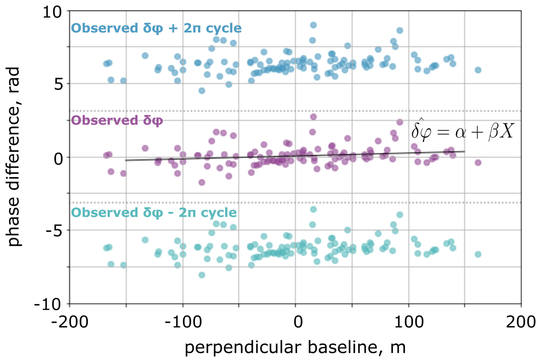
Figure 2 Example of correlation between phase and perpendicular baseline for one moving window. Each purple point represents the complex average phase in the sample window for a given interferogram with respect to the complex average phase in the reference area. As the phase is known in modulo 2π, its +2π and −2π values are also shown in blue and teal respectively. (Modified from Dini et al., 2022, Gretsi Colloque Proceedings.)

3.3 Coherence loss analysis

Interferometric coherence and its changes within the landslide and in the surrounding area were analysed both in space and time, in a qualitative and quantitative way respectively. We retained all the selected 113 successive interferograms for this analysis, irrespective of their average coherence. This is because if coherence is to be used as a precursory indicator, its potential should be tested over a range of interferograms, including those in which the phase might be unreliable. Spatial coherence loss is identified within individual interferograms. We focused on patterns of coherence loss over confined areas, as a proxy of localised strain: localised and spatially organised changes of the complex interferometric values are likely associated with localised displacements, particularly if these correspond to gravitational morphological features (e.g. scarps or extensional structures associated with gravitational slope movements). The coherence images can be found in Dini et al. (2025b).

In order to detect changes in mean coherence through time and between the landslide and the surrounding gravitationally stable areas, we first calculated for each interferogram the average coherence over the whole crop, along the scarp and within the mapped landslide boundaries. The scarp and crown areas are key locations for precursory detection as motion related to retrogression might be focused here. Boundaries for the scarp were mapped on Google Earth optical images on the basis of geomorphological features and then converted in radar coordinates, as for the landslide boundaries. We analysed the average coherence time series in relation to daily rainfall, downloaded from the online platform of the national service of Meteorology and Hydrology of Peru (Servicio Nacional de Meteorología e Hidrología del Perú, 2023) (see Sect. 3.6.2 for further details). We then computed the time series of the ratio between average landslide coherence and average coherence of the surrounding area (Jacquemart and Tiampo, 2021). The ratio is chosen because it highlights changes occurring in the landslide with respect to the surroundings, whilst accounting for periods of coherence loss associated to vegetation changes or ground moisture changes due to rainfall events that would affect the coherence everywhere in a similar way. The changes highlighted by such ratio are therefore most likely associated with ongoing deformation inside the landslide area. In our method, coherence is interpreted relative to a local surrounding area rather than across a large region or the entire SAR frame. As mentioned in Sect. 3.1, we selected the size of the surrounding area so that it is comparable to the landslide footprint, serving as a baseline for normal variability, but not too large to avoid including very different noise sources. Thus, this approach does not require the landslide to stand out across a much larger area; rather, the key signal emerges from local deviations detectable over a few km scale. A temporal mean coherence was computed for each pixel and compared to background terrain using z scores (see the Supplement and Fig. S9).

3.4 Wrapped phase analysis

As explained in Sect. 1, the presence of interferograms with a high displacement gradient and/or low $S/N$ ratio hinders the ability to perform reliable phase unwrapping without errors during phases of landslide acceleration. We thus adopted the following procedure to analyse the wrapped phase signal in time, whilst avoiding phase unwrapping. Following an approach similar to that presented in López-Quiroz et al. (2009), we selected 5 interferograms characterised by high $S/N$ ratio and by relatively low displacement gradients. In particular, we ensured to select only interferograms in which the observed displacements gradients would not exceed 2π over the landslide area. The visual inspection of all wrapped interferograms revealed that the area affected by displacements has a similar spatial pattern until failure and that the displacement gradient, as observed in interferograms with higher $S/N$ ratio, has the same sign throughout (which is expected in gravitational motion). For the five chosen interferograms we added 2π to all pixels with phase value < −1 rad, thus obtaining a pattern with values comprised between −1 and 5.28 rad. We then averaged these interferograms, obtaining what we will refer as a model deformation pattern (Fig. 3A). We cut the area closely around the deformation pattern over 33 × 33 pixels, in order to reduce the contribution of noise in the surrounding area. We then used this model pattern to investigate its correlation with all 113 interferograms in the series, so that:

$$\begin{array}{}\text{(4)}& \mathit{\alpha }{e}^{i{\widehat{\mathit{\delta }\mathit{\phi }}}_{k,p}}=e^{i{M}_p{\mathit{\alpha }}_k},\end{array}$$

where $e^{i{\widehat{\mathit{\delta }\mathit{\phi }}}_{k,p}}$ is the predicted phase value at pixel p of interferogram k, M_p is the phase value of the model deformation pattern at pixel p and α_k is the proportionality coefficient between the phase of the model pattern and interferogram k (Fig. 3B). For the parameter search, −7 and 7 were chosen as bounds for α_k, to account for potentially large displacements that might have affected the landslide in the days/weeks before failure, with a 0.001 step. The value of the proportionality coefficient α_k is then used to represent a dimensionless measure of displacement rates, DI, which is a quantity of activity for each interferogram in the series. For example, interferograms characterised by α_k around zero are those with no detectable displacements, whilst α_k around 1 would indicate for interferogram k a similar displacement gradient to the model pattern. The value of α_k is obtained by maximising the coherence between the predicted and observed values, the latter a measure of the goodness of fit:

$$\begin{array}{}\text{(5)}& {\mathit{\gamma }}_k=\left|{\displaystyle \frac{{\sum }_k{e}^{i{\mathit{\phi }}_{k,p}}\cdot {e^{i{\widehat{\mathit{\delta }\mathit{\phi }}}_{k,p}}}^{\ast }}{N_p}}\right|,\end{array}$$

where N_p is the number of pixels in interferogram k. Successively, the same procedure was applied only to pixels falling within the landslide, masking outside pixels. This was done to generate a ratio between the best coherence calculated over landslide pixels only and the coherence over all pixels, including surrounding area pixels. A low ratio indicates poor fit of the model within the landslide area in particular, which in turn indicates high likelihood of high displacements gradients leading to spatial aliasing and decorrelation. A threshold of such ratio was set at one standard deviation below the mean value. Unreliable interferograms (grey dots in Fig. 6) are those with ratio falling below this threshold. The code to perform this analysis can be found in Dini et al. (2025a).

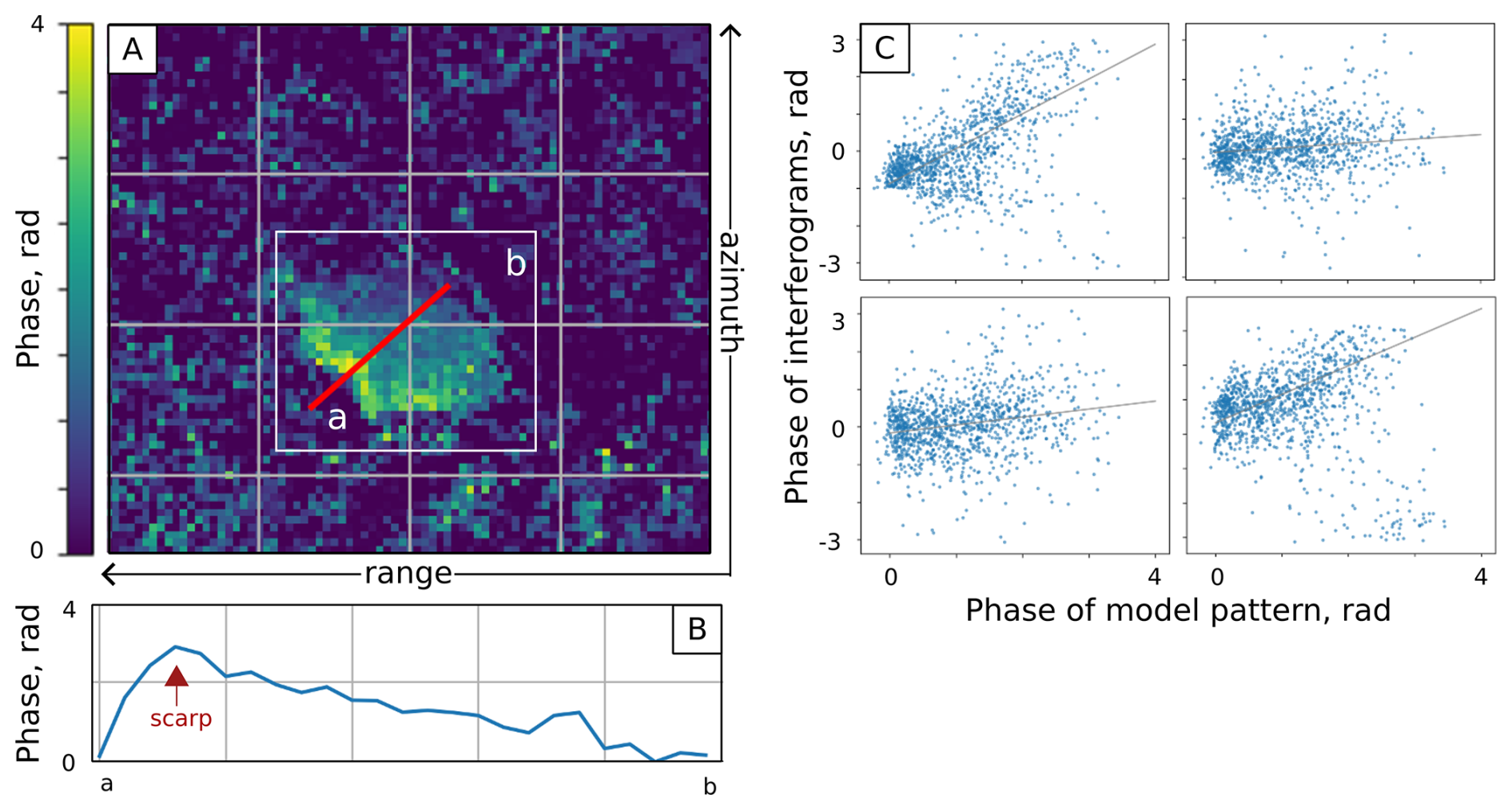
Figure 3 (A) Model pattern of deformation in radar coordinates (flipped left-right); (B) model pattern phase gradient for the profile a–b; (C) examples of four interferograms showing the pixel-by-pixel correlation with the model pattern (from top left, clockwise: 18–30 August, 30 August–11 September, 23 September–5 October, and 5—29 October 2018).

3.5 InSAR-derived downslope displacements

The dimensionless measure of displacement rates, DI, obtained with the analysis of raw phase in successive interferograms described in Sect. 2.4 is not an absolute measure of displacements. It represents the degree of activity within the landslide in the time interval covered by each interferogram, as it reflects the correlation between the model pattern and each interferogram. Figure 3C shows a profile across the model that runs along the maximum slope gradient roughly, through the middle of the landslide. The highest values are observed at the scarp, with a maximum value, r_max, of 3.45 radians, decreasing to around zero at the toe of the landslide. Therefore, to estimate line of sight (LOS) displacements in mm, we rescaled the dimensionless displacement rates, DI, as:

$$\begin{array}{}\text{(6)}& {\text{DI}}_{\mathrm{mm}}=\text{DI}\cdot r_{max}\cdot {\displaystyle \frac{\mathit{\lambda }}{\mathrm{2}\mathit{\pi }}},\end{array}$$

where λ is the half the wavelength of the satellite, which for Sentinel-1 is 28 mm.

An assumption generally accepted for landslides is that the displacement vector is oriented along a line of maximum slope gradient (Notti et al., 2012). This reflects the overall motion of the landslide, even if, unless the landslide is a pure translational slide, some parts of compound landslides have higher vertical component of the displacements than others. Following the approach presented in Notti et al. (2012), we computed a coefficient that describes the percentage of downslope displacement that is detectable along the line of sight and applied a correction to the displacements. This coefficient is 0.88, for an incidence angle over the area of 40.7°, a heading angle of 347°, and average slope and aspect of 17 and 74° respectively.

We then applied a correction to the displacements obtained with the optical image correlation, DO, described in Sect. 2.4, once again assuming that the displacements occur along the maximum slope gradient and taking an average slope angle of 20°, so that:

$$\begin{array}{}\text{(7)}& {\text{DO}}_{\mathrm{mm}}={\displaystyle \frac{\text{DO}}{\sin \left(\mathit{\vartheta }\right)}},\end{array}$$

where ϑ is 70°, the complementary to the average slope angle. The code to derive the displacement estimates can be found in Dini et al. (2025a).

Finally, we identified the onset of activity periods in the InSAR time series, we fitted for each period a linear model. We then computed the slope of the curve for each phase and compared the values at different ones.

3.6 External forcing

In order to detect external events that may have played a role in the onset of activity at specific times, we took into consideration seismicity, rainfall and maximum river width as a proxy for erosion. The pore pressure increase associated with rainfall (Agliardi et al., 2020; Carey et al., 2019) and seismic shaking (Lacroix et al., 2022) is an important factor that perturbs the internal stress state of the rupture surface of large landslides, inducing slip onset (Agliardi et al., 2020). River erosion also plays a role in modulating landslide activity in the region (Lacroix et al., 2015) and increased fluvial erosion might increase landslide activity by removing material at the toe (McColl, 2022), undercutting the slope (Ballantyne, 1986; Fourniadis et al., 2007; Yang et al., 2021) and potentially exposing the sliding surface.

3.6.1 Earthquakes

We computed a comprehensive list of earthquakes with magnitude 3 and above, occurred within a radius of 150 km of the Achoma landslide, between 2015 and July 2020 from the online platform of the Geophysical Institute of Peru's (Instituto Geofísico del Peru, 2022). The list comprises of 361 events. For each event, we calculated the expected peak ground acceleration (PGA, m s⁻²) as indicator of seismic ground motion at the Achoma landslide site by applying the ground motion prediction method of Akkar and Bommer (2010). This method was shown by previous studies to perform well for a landslide site located approximately 10 km west of the Achoma landslide (Bontemps et al., 2020; Lacroix et al., 2015). PGAs of 0.1 m s⁻² and above are obtained for earthquakes occurred at less than 50 km from the landslide, with magnitudes comprised between 3.8 and 5.6, except for one event, occurred at 84 km, but with magnitude 6.2. The earthquake data used can be found in Dini et al. (2025a).

3.6.2 Rainfall

Hourly rainfall data starting from 2015 recorded at the station of Chivay, approximately 9 km northeast of the landslide site, at a similar elevation, were downloaded from the online platform of the National Service of Meteorology and Hydrology of Peru (Servicio Nacional de Meteorología e Hidrología del Perú, 2023). This was then converted into daily rainfall totals. Cumulative rainfall for each dry-rainy season sequence (August to August of following year) has been plotted for every year, to compare activity rates with rainfall. 2015 and 2016 were characterised by drier conditions than following years. To identify more intense daily rainfall events, characterised by higher 24 h cumulative rainfall, we computed the histogram of daily rainfall, which presents a skewed right distribution. We selected a threshold of 25 mm d⁻¹ as the intense rainfall event, as frequencies of higher daily totals do not exceed 1 in the whole observation period. The rainfall data used can be found in Dini et al. (2025a).

3.6.3 River erosion

As a proxy for river erosion at the landslide's toe, we analysed the changes in river width over time. To accomplish this, we utilised 219 Planet Lab PlanetScope images with 3 m ground resolution. We selected three sections along the river: one in the middle of the landslide and one at each boundary. For each image, we measured the river's width at each of the three locations. The river's width broadly follows a seasonal pattern corresponding to the seasonal rainfall over the area, implying that the river's erosive power follows a similar temporal pattern to the rainfall. However, our objective was to identify unseasonably large river events that might be triggered by localised events upstream in the catchment, which are not directly recorded at the nearby meteorological station. To identify such unseasonable events, we computed a rolling mean of the river width and looked for peaks exceeding 1 standard deviation from the mean. In addition to this, we mapped the riverbanks at maximum width for each year, to determine any position changes through time that might be indicative of persistent, significant erosion. The river width data compiled in this work can be found in Dini et al. (2025a).

4 Results

4.1 Spatial coherence features as long-term precursors

Interferometric coherence maps generated for all selected successive interferograms (see Sect. 2) exhibit distinct, consistent features over the observation period (Fig. 4). Notably, low coherence lineaments appear intermittently up to 5 years before the landslide failure. These features manifest as narrow, rope-like structures located primarily along the scarp and southeastern flank of the landslide, consistent with post-failure observations. Interestingly, these features persist even in interferograms characterised by generally low coherence, where phase unwrapping would typically be unreliable. They are identifiable in 25 interferograms spanning from the earliest available (covering the period 30 April to 11 July 2015) up until 16 March 2020, approximately 3 months prior to the failure. Pixels intersecting the scarp exhibit significantly lower coherence than the surrounding area (Welch's t test, p < 0.001; see the Supplement and Fig. S9). Starting from 9 April 2020 the entire area affected by the landslide shows a more widespread loss of coherence, indicative of a regime shift.

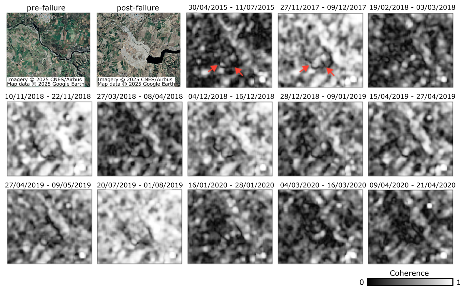
Figure 4 Pre-failure image (date: 29 April 2019) and post-failure image (date 1 November 2020) with a series of interferometric coherence examples showing the development of headscarp and southern boundary, with the change in regime from March 2020. Pre- and post-failure Imagery © 2025 CNES/Airbus, Map data © 2025 Google Earth.

4.2 Time series of coherence ratio

Figure 5A illustrates the average coherence in the landslide area and in the surrounding area. Albeit with some small differences, the coherence drops everywhere following similar temporal patterns during the rainy seasons. The coherence ratio between the landslide and the surrounding area (Fig. 5B) remains around 1, with a mean of 0.98, from 30 April 2015 to 28 March 2020, encompassing multiple wet seasons. Subsequently, starting from this date until the failure on 18 June 2020, the ratio progressively declines below 0.8, reaching its lowest value of 0.19 at the time of failure. The significant drop in the coherence ratio 3 months prior to failure indicates that the landslide area was losing coherence faster than its immediate and directly comparable surroundings.

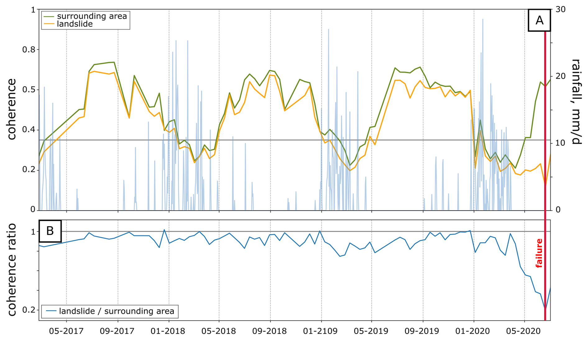
Figure 5 (A) Interferometric coherence for different parts of the landslide, superposed on daily rainfall. (B) Coherence ratio. Failure is indicated by the vertical red line.

4.3 Acceleration phases as seen by InSAR

The dimensionless activity index time series, derived using the method outlined in Sect. 2.5, is shown in Fig. 6. The time series reveals periods of relative stability interspersed with phases of acceleration. Transient creep events are characterised by displacements occurring within individual or, in one case, over two consecutive interferograms amid periods of minimal long-term displacements. Four transient creep events between April 2015 and August 2016 exhibit dimensionless displacement rates exceeding 1, occurring amidst a backdrop of rates generally around 0 and less than 0.25 (Fig. 6; Table 1). The displacements observed in these interferograms match or exceed the mean deformation pattern shown in Fig. 3A. In contrast, we observe long acceleration phases, periods during which displacement rates increase significantly over three successive interferograms or more. These become apparent from November 2017 onwards.

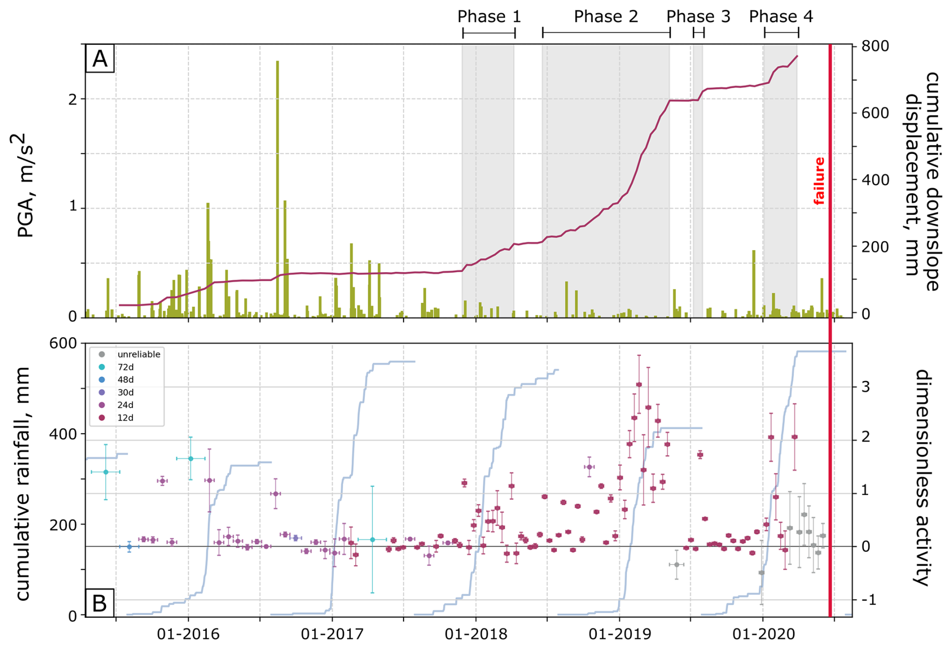
Figure 6 (A) Purple curve, estimated downslope cumulative displacement in mm after correction; green bars, PGA. (B) Dimensionless activity index, every dot represents an interferogram, different colours and horizontal bars represent interferogram duration, vertical bars $\mathrm{1}/{\mathit{\gamma }}_k$ normalised by its max value (Eq. 5); blue curves, cumulative rainfall over the rainy season.

Table 1 Interferograms showing possible transient creep behaviour associated with nearby earthquakes.

Four distinct acceleration phases are observed:

• Phase 1: 27 November 2017, to 8 April 2018

• Phase 2: 19 June 2018, to 9 May 2019

• Phase 3: 8 July 2019, to 20 July 2019

• Phase 4: 4 January 2020, to 4 March 2020 (culminating in failure 3 months later)

The accelerations are detected using the dimensionless index (see Sect. 2.4), but we present below the estimated rates (see Sect. 2.5), for ease of description.

The first acceleration begins with an initial significant displacement (∼ 18 mm in 12 d), followed by a period of linear displacements over 132 d at an almost steady rate of approximately 279 mm yr⁻¹.

The second phase follows a 10-week quiescence period and exhibits escalating trends: 234 mm yr⁻¹ between 19 June and 5 October 2018; 425 mm yr⁻¹ between 5 October 2018 and 9 January 2019; and 1080 mm yr⁻¹ between 9 January and 9 May 2019.

A short acceleration in July 2019 transitions quickly into a brief period stability followed by a phase of low, steady-rate creep from 1 August to 23 December 2019, characterised by a gentle trend of 38 mm yr⁻¹. This is succeeded by the last acceleration phase, reaching approximately 567 mm yr⁻¹ from 4 January to 4 March 2020, the last reliable interferogram captured, then culminating in failure.

5 Discussion

5.1 Spatial patterns of low coherence

The coherence maps derived from successive interferograms reveal slope instability by delineating gravitational morphological structures dating back 5 years before failure. In the earliest available interferogram (30 April–11 November 2015), a distinct low coherence boundary is evident despite the low average coherence, closely mirroring the later spatial development of the landslide. The low-coherence markers likely indicate areas of strain resulting from landslide displacement, marking the boundary between stable and unstable ground. These markers are interpreted as early signs of destabilisation, suggesting strain concentration along the failure surface is beginning to occur, albeit with very small displacements. We observed similar features in other landslides in the Colca Valley, indicating that these signals are not isolated occurrences and highlighting their importance and reliability for early detection at large scales. Some of these landslides have exhibited long-term creep without progressing to catastrophic failure. In these cases, low-coherence markers appear to indicate retrogressive behaviour with the formation of secondary scarps over the years and delimiting different activity sectors.

5.2 Factors influencing coherence loss

Low interferometric coherence, reflecting high phase variability between adjacent pixels, can be caused by factors like dense vegetation, crops, surface debris, snow, or spatial heterogeneity of ground deformation. In the case of the Achoma landslide, the low coherence markers observed are unlikely to be caused by localised land cover changes. Instead, they likely reflect slight differential displacements associated with the development of surface discontinuities. These features have been observed up to 3 months before failure, similar to the final acceleration stage detected with optical images by Lacroix et al. (2023). Jacquemart and Tiampo (2021) discuss various factors contributing to interferometric coherence loss in landslides, including soil moisture changes, erosion, vegetation dynamics, and active slope deformation. While distinguishing between these causes is challenging, their combined presence suggests increased landslide activity.

The observed transition in coherence patterns, from localised anomalies along gravitational structures to widespread loss across the entire landslide area in March 2020, points to significant shift in landslide dynamics. This likely marks the transition from small displacements (with the landslide behaving as a cohesive body) to higher displacement gradients and internal deformation. Identifying such transitions in coherence could provide valuable lead time for early warnings, offering a proactive approach to landslide monitoring in previously unmonitored areas.

5.3 Coherence ratio analysis

In addition to the spatial patterns of low coherence, we analysed the ratio between the mean coherence over the landslide area and that in the surrounding area, using a methodology similar to that adopted by Jacquemart and Tiampo (2021). This ratio helps account for temporal coherence variability that affects both the landslide and its surroundings similarly. For example, seasonal moisture changes can impact coherence, but the ratio remains close to 1 unless changes occur specifically within the landslide area.

A noticeable drop in the coherence ratio occurred approximately 3 months before the failure event, beginning around 4 March 2020. By setting a retrospective threshold (1 standard deviation below the mean coherence ratio), we identified that this threshold was surpassed between 9 and 21 April 2020, indicating predictive value about 2 months before the Achoma failure. Jacquemart and Tiampo (2021) noted a similar coherence ratio decline approximately 5 months before the Mudcreek landslide, attributing it partly to vegetation degradation. In contrast, our analysis of the Achoma landslide shows a sharp increase in the coherence ratio post-failure, reaching values as high as 1.98 during the 2021 rainy season. This increase suggests that vegetation degradation following the failure may expose rock and soil, enhancing phase stability in the absence of displacements. Thus, the observed drop in coherence leading up to failure is likely associated with high displacement gradients leading to increased internal deformation of the landslide mass and phase aliasing. This observation is consistent with the 3-month final acceleration stage identified through independent measurements by Lacroix et al. (2023). Further investigation into other case studies is needed to establish universal indicators and thresholds for landslides at critical stages.

5.4 Dimensionless activity index

The InSAR data processed in this work indicates that the Achoma landslide underwent a long evolution. Our observations show that progressive damage and fault maturation over a period of at least 5 years, likely longer, ultimately led to landslide failure, in agreement with the findings of Lacroix et al. (2023). To simplify, we separately discuss two broad periods, based on different styles of activity observed.

5.4.1 April 2015 to December 2017

The key observation is that between April 2015 and December 2017 the long-term activity index for this period reveals short-lived transient creep events in response to perturbations, interspersed with prolonged period of little to no activity (Fig. 6; Table 1). This suggests the presence at this stage of a maturing surface of rupture, allowing for some hydro-mechanical fluid-solid coupling (Agliardi et al., 2020), but not yet a self-sustaining process of progressive failure. Displacements during this period may span up to 72 d due to sampling intervals. Between December 2015 and March 2016, a combination of moderate seismicity and rainfall led to possible prolonged displacements over two consecutive interferograms for up to 96 d. However, the temporal resolution of the data does not allow us to determine whether movement was continuous or intermittent within these intervals.

While the August 2016 earthquake, with the highest PGA of 2.34 m s⁻² recorded during the study period, did result in some movement, it was lower than the movements observed between April 2015 and March 2016. Moreover, although the rainy season of 2016/2017 recorded comparable precipitation totals to subsequent seasons, no prolonged period of acceleration was observed until the end of 2017. This suggests that a combination of seismicity and rainfall may be more critical for driving significant acceleration than either factor alone. Unlike the Maca landslide, which exhibited prolonged post-seismic accelerations following the 20 February and 15 August 2016 earthquakes, lasting 5 months and several weeks, respectively (Bontemps et al., 2020), the Achoma landslide's response was transient and not sustained, as no subsequent interferograms indicated continued movement. Post-seismic motion has been associated to pore-water pressure increases due to sediment contraction (Lacroix et al., 2022). The absence of post-seismic motion at the Achoma landslide may reflect that the rupture surface was not sufficiently mature, and lacked the necessary pathways for water to migrate from contracted sediments to the rupture zone. Without this migration, the pore pressure at the rupture surface could not build up to a level that would sustain post-seismic motion.

5.4.2 December 2017 to June 2020

A shift in behaviour can be identified from December 2017: from this point, longer periods of activity begin to occur. The landslide reacts quickly to the onset of the wet season in December 2017, despite lower seismicity than in the previous period, suggesting that the rupture surface has fully developed and become more sensitive to perturbations. This likely reflects the formation of a fine-grained gouge along the basal shear plane (Agliardi et al., 2020), reducing permeability and altering pore pressure dynamics. These internal changes led to cycles of acceleration, deceleration, and steady-state stages (Zhou et al., 2018) (Fig. 6A), driven by transient perturbations like seismic events or rainfall and modulated by mechanisms like pore pressure dissipation (Lacroix et al., 2020) or strain-strengthening behaviour (Agliardi et al., 2020) ultimately resulting in sustained slip rates even during dry periods. This pattern is particularly evident during the dry season of 2018, when the Achoma landslide exhibited sustained displacement rates despite the absence of significant external triggers. This observation highlights the role of ongoing internal processes, such as continued damage accumulation along the basal shear plane, in maintaining instability and movement over time.

As Lacroix et al. (2023) note, the final stage of acceleration began in the wet season. While optical images from Lacroix et al. (2023) pinpoint the beginning of the final acceleration in March 2020, InSAR-based observations in this study suggest that the landslide began accelerating as early as January 2020, following a period of steady slip rates during 2019. Although rainfall was undoubtedly a key factor, similar rainfall totals in 2017 and 2018 did not lead to failure, suggesting that other factors, such as accumulated damage or changes in the basal shear zone, were more critical in 2020. Increased seismic activity in the final stages, marked by a higher frequency of smaller earthquakes, likely contributed to the landslide's acceleration, demonstrating a combination of driving factors.

Figure 7 compares acceleration phases 1, 2, and 4 using inverse velocity (d mm⁻¹) plots, derived from the estimated displacements. Although the measure is not an absolute displacement, its evolution reflects distinct kinematic behaviours. Phase 1 begins at a high inverse velocity (> 100 d mm⁻¹), indicating very slow initial movement and a large relative change during acceleration. Phases 2 and 4 start from lower $\mathrm{1}/v$ values, suggesting a more active baseline state by the time acceleration began. Phases 1 and 2 show an abrupt initial drop followed by flattening at values above zero, consistent with asymptotic decay and indicating the attainment of temporary steady states following transient accelerations (Carlà et al., 2017). In contrast, phase 4 declines more gradually but approaches near-zero inverse velocity within ∼ 3 months, signalling sustained acceleration towards failure rather than stabilisation. This pattern suggests the slope did not fully recover stability between acceleration episodes, supporting the interpretation of progressive internal degradation and gradual accumulation of strain.

Figure 7 (A) 1/velocity plots for phase 1, phase 2, and phase 4. (B) Displacement rates for raw (black dots) and smoothed data (blue x, smoothed using a 5-window running mean). Shaded areas show accelerations of phase 1, phase 2 and phase 4.

While external forcing factors, such as rainfall and seismic activity, modulated the timing and magnitude of these accelerations, they cannot alone explain the observed behaviour. For instance, comparable rainfall totals in 2019–2020 did not trigger failure, and acceleration continued through the 2018 dry season. The $\mathrm{1}/v$ plots highlight the internal process of material degradation, including microcrack formation and coalescence, leading to the development of a shear surface by March 2020. By observing these behaviours, we demonstrate how dimensionless parameters from the wrapped phase can capture meaningful kinematic evolution, offering valuable insight into early destabilisation mechanisms.

Finally, it is worth noting that phase 4 is truncated roughly 3 months prior to failure due to increasing noise in the dimensionless measure, preventing observation of the full $\mathrm{1}/v$ trend as the landslide approaches collapse. These inverse velocity plots are therefore not intended to predict failure timing but to illustrate the changing kinematic behaviour across acceleration phases.

Figure 8A shows the position of the riverbanks during maximum river width periods for each wet season (2016–2020). Despite potential image resolution limitations, our observations reveal no clear trend of significant erosion toward the left bank or landslide toe. Instead, riverbank positions vary over time, indicating movement in both directions, into and away from the landslide toe. The right bank shows a slight tendency to move away, possibly due to the landslide toe pushing the riverbed, which may increase erosion on that side. River width measurements in Fig. 8B–D, used as a proxy for erosional power, do not indicate significant erosion events during the 2020 dry season. These findings suggest that the landslide was not triggered by high river erosion, but rather by a long-term process of progressive failure.

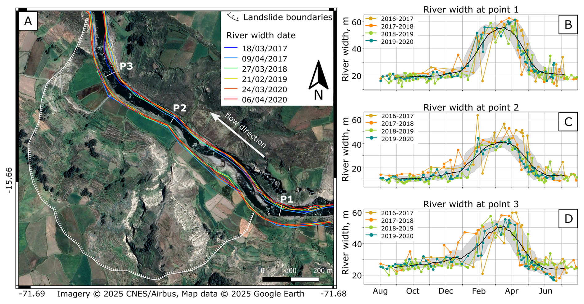
Figure 8 (A) Mapping of riverbanks position at maximum width. If date of maximum width differs between P1, P2, P3, multiple dates per wet season are taken (e.g. 2017, 2020). Mapping and annotations are superposed to a satellite image for 20 April 2019 (Imagery © 2025 CNES/Airbus, Map data © 2025 Google Earth). (B–D) River widths for P1, P2, P3 respectively. Data is plotted from dry season to dry season the following year. The black curve represents the 40 d running mean, and the grey shading represents 1 standard deviation above and below the mean.

5.5 Complementarity

Our observations highlight variations in the Achoma landslide's response to triggers, depending on its stage of basal shear plane maturation, suggesting that different processes were involved. We retrospectively identify the beginning of a final acceleration already in January 2020 (as shown by wrapped phase dimensionless activity marker), transitioning into a critical and irreversible instability in March 2020 (as shown by coherence both in space and time), indicating that proactive monitoring could have commenced at least at this critical stage. This finding echoes Jacquemart and Tiampo's (2021) observation of a coherence ratio drop 5 months before the failure of the Mudcreek landslide, emphasising its potential as early indicator. They also noted that an approach based on time series generation underestimated displacements. In contrast, (Handwerger et al., 2019) used a preprocessing step for signal removal before unwrapping in their analysis of the same landslide. Our method, leveraging wrapped phase analysis, offers a more streamlined alternative, providing valuable insights into landslide evolution without complex preprocessing. Unlike traditional InSAR approaches requiring signal removal and reintroduction, our method is less time-consuming and demonstrates the effectiveness of analysing the wrapped phase. In addition to this, integrating InSAR-based signals with optical time series enhances the understanding of landslide dynamics across different phases. The metrics we propose identify areas of incipient strain and early acceleration phases, while optical time series capture the final acceleration phase characterised by larger displacements (Fig. S10).

The indicators proposed here rely on the identification of critical features, such as gravitational structures in the coherence signal or the moving mass in the wrapped phase. In practice, wrapped phase patterns could also be used to delineate the boundaries of potentially unstable zones, which can serve as the basis for coherence ratio analyses to assess localised changes relative to their surroundings. While the observed coherence and phase signals are promising indicators, determining whether they can be reliably detected without prior knowledge of landslide locations will require large-scale analysis across diverse terrains, likely combining InSAR with topographic, geomorphic, and signal-specific characteristics. Evaluating the generalisability of this methodology across different landslide types and settings is a key goal for future work. Furthermore, automated detection of these features using machine learning techniques could significantly enhance landslide monitoring. Approaches such as that proposed by Chen et al. (2022) demonstrate the feasibility of applying deep semantic segmentation to recognise active landslides from InSAR. Implementing similar AI-driven frameworks on the precursors identified here could automate the detection of early instability signs, reducing reliance on manual interpretation and providing an efficient first filter for identifying destabilising slopes across large areas. Finally, the approach proposed here could be highly complementary to recent optical monitoring methods aimed at detecting slow-moving landslides. For instance, Van Wyk de Vries et al. (2024) demonstrated that automated Sentinel-2 feature tracking can identify surface deformation for landslides attaining larger velocities than InSAR can detect, providing valuable information on spatial displacement patterns where optical contrast and cloud-free conditions permit. In contrast, InSAR-based coherence and wrapped-phase indicators may be more sensitive to subtler or intermittent deformation and are less dependent on illumination or atmospheric conditions. Furthermore, it is worth noting that the rates of ground deformation detectable with InSAR and optical vary significantly, allowing for the detection of different phases, as shown in this work. Integrating both datasets could therefore improve the detection of a broader spectrum of slope processes, from slow or incipient deformation to more rapid movement phases and enhance confidence in precursor identification by combining independent observational evidence.

6 Conclusions

Using Sentinel-1 interferograms with non-overlapping short temporal baselines, we identified precursors to the Achoma landslide. Our approach bypasses traditional unwrapping and time series generation, revealing significant spatial coherence loss that indicates gravitational features linked to strain localisation along the rupture surface, visible 5 years prior to failure. Intermittent coherence loss from approximately 5 years to 5 months before failure suggests the progressive development of a hydro-mechanically coupled rupture surface with increasing damage concentration. This is further supported by the acceleration, steady-state, and deceleration phases observed in the wrapped phase analysis. Our findings demonstrate the potential of satellite-based InSAR to detect destabilisation precursors before large displacements occur, particularly when continuous displacement time series are hindered by land cover or landslide behaviour. By integrating key parameters and their spatiotemporal changes, this methodology could enhance the identification of precursors over larger areas than traditional time series methods alone, making satellite-based monitoring even more valuable for landslide prediction. However, we acknowledge that not all landslides exhibit measurable precursory motion. For example, rapid, shallow failures in unconsolidated materials may occur with little to no detectable warning. The approach presented here is therefore likely applicable to large, complex landslides with long histories of slow deformation for which strain accumulation can be capture, and further research across a broader range of case studies is needed to validate coherence loss patterns as reliable precursors for landslides with minimal ground displacement. In this context, a key next step will be to extend this work to regional studies to capture landslides in diverse geological and climatic settings, with different sizes, mechanisms and material composition, to determine more broadly under which conditions similar precursory patterns would emerge and how can they be objectively characterised.

Our findings are nevertheless significant for two practical reasons. First, the Achoma landslide went unnoticed until shortly before failure, a common issue in landslide science where monitoring typically begins after events occur rather than during early precursor stages. Identifying reliable precursors in satellite data could improve landslide prediction on both local and broader scales. While our analysis demonstrates the potential for satellite-based detection of precursory signals, effective early warning ultimately depends on coupling such remote observations with local monitoring and community awareness. Second, the challenge of monitoring landslides only after failure limits the capture of earlier instability phases. Proactively targeting destabilising slopes for instrumentation is critical for effective hazard assessment, failure prediction, and understanding underlying processes. A complementary approach that combines the strengths of InSAR and optical time series, while leveraging AI for automated feature detection, holds remarkable potential for advancing real-time landslide monitoring. Such innovations are key to enhancing community resilience by enabling early detection and supporting timely response and preparedness in landslide-prone regions.