Emergence of climate change signal in CMIP6 extreme indices

Climate and weather extremes are becoming more frequent due to the influence of anthropogenic climate change. Knowing when and where we can expect these changes to occur is essential for both climate change mitigation and developing adaptation measures. We investigate the time of emergence – meaning the earliest time at which the climate change signal can be detected from the noise of natural variability – for 27 annual and 2 seasonal climate extreme indices related to surface temperature and precipitation. An ensemble of 21 CMIP6 global climate models (including several with a large number of initializations) is combined with a model weighting scheme that accounts for both model performance and independence to provide robust ensemble statistics of the emergence of climate extremes and to explore model uncertainty.

Results indicate that spatial and temporal emergence patterns differ between types of temperature indices, for instance we find that percentile-based indices emerge earlier than their absolute counterparts. Indices related to daily maxima tend to emerge later than those related to daily minima. For many temperature indices, emergence occurs during the historical period (before 2015) and first in tropical regions with the exception of annual minimum indices, which show a more spatially uniform pattern.

Precipitation indices tend to emerge later (mostly after 2030), only in some parts of the globe and/or primarily under high emissions scenarios. Some indices show spatial variations in the sign of change, although both positive and negative changes can lead to emergence. The main regions of emergence are the northern high latitudes and central Africa, however there is substantial disagreement between models about whether or not emergence occurs elsewhere.

The results of this study provide a consistent basis for understanding and comparing the emergence of different types of extremes, and they highlight opportunities for further research into the underlying drivers, as well as impact- or region-specific risk assessments.

1 Introduction

Understanding the concept of climate emergence and identifying the emergence for climate extremes is crucial for both adaptation and mitigation strategies. According to IPCC (2021c), climate emergence refers to the appearance of new conditions in a climate variable within a region, often measured by the ratio of change relative to natural variability (signal-to-noise ratio). Emergence occurs when this ratio surpasses a defined threshold and can be expressed as the time or global warming level at which these changes first appear, estimated using observations or model simulations. While earlier studies primarily focused on mean climate variables, such as average temperature and precipitation (Diffenbaugh and Scherer, 2011; Hawkins and Sutton, 2012; Mahlstein et al., 2011, 2012a, b; Nguyen et al., 2018), the most severe climate impacts are often linked to extreme events (IPCC, 2022). Evidence shows that the intensity and frequency of extreme temperature and precipitation events have already increased compared to the preindustrial climate and these changes are attributable to human activities (IPCC, 2021b; King et al., 2016). Particularly, least or less developed countries are more likely to experience emergence of temperature extremes, since many are located in low latitude regions with low temperature variability (Harrington et al., 2016; King et al., 2023; Gampe et al., 2024; Iles et al., 2024).

Mean temperatures and heat extremes have emerged with high confidence above natural variability in almost all land regions (IPCC, 2021b; King et al., 2015), however climate variability plays a major role in determining the timing and extent of emergence (Hawkins et al., 2020). While uncertainty in global mean temperature projections is mainly driven by differences between models and scenarios, regional temperature trends are significantly more influenced by internal climate variability. To address this, Single Model Initial Condition Large Ensembles (SMILEs) have been developed to sample this variability more robustly (Kay et al., 2015; Maher et al., 2019; Lehner et al., 2020). Internal variability also contributes significantly to the delayed emergence or lack of emergence of the anthropogenic signal in long-term regional mean precipitation changes (IPCC, 2021c), as demonstrated by multiple lines of evidence such as global projections from multi-model ensembles and SMILEs.

CMIP6 (Coupled Model Intercomparison Project Phase 6; Eyring et al., 2016) provides a large ensemble of models – with several individual models comprising 10 or more ensemble members themselves – thus offering a more comprehensive basis for capturing climate variability as compared to just a single model. However, to reduce biases and obtain accurate uncertainty estimates from multi-model ensembles, model weighting should be considered (Knutti et al., 2013, 2017), for example the approach introduced by Brunner et al. (2020b), which accounts for historical model performance and interdependence between models in the CMIP6 ensemble.

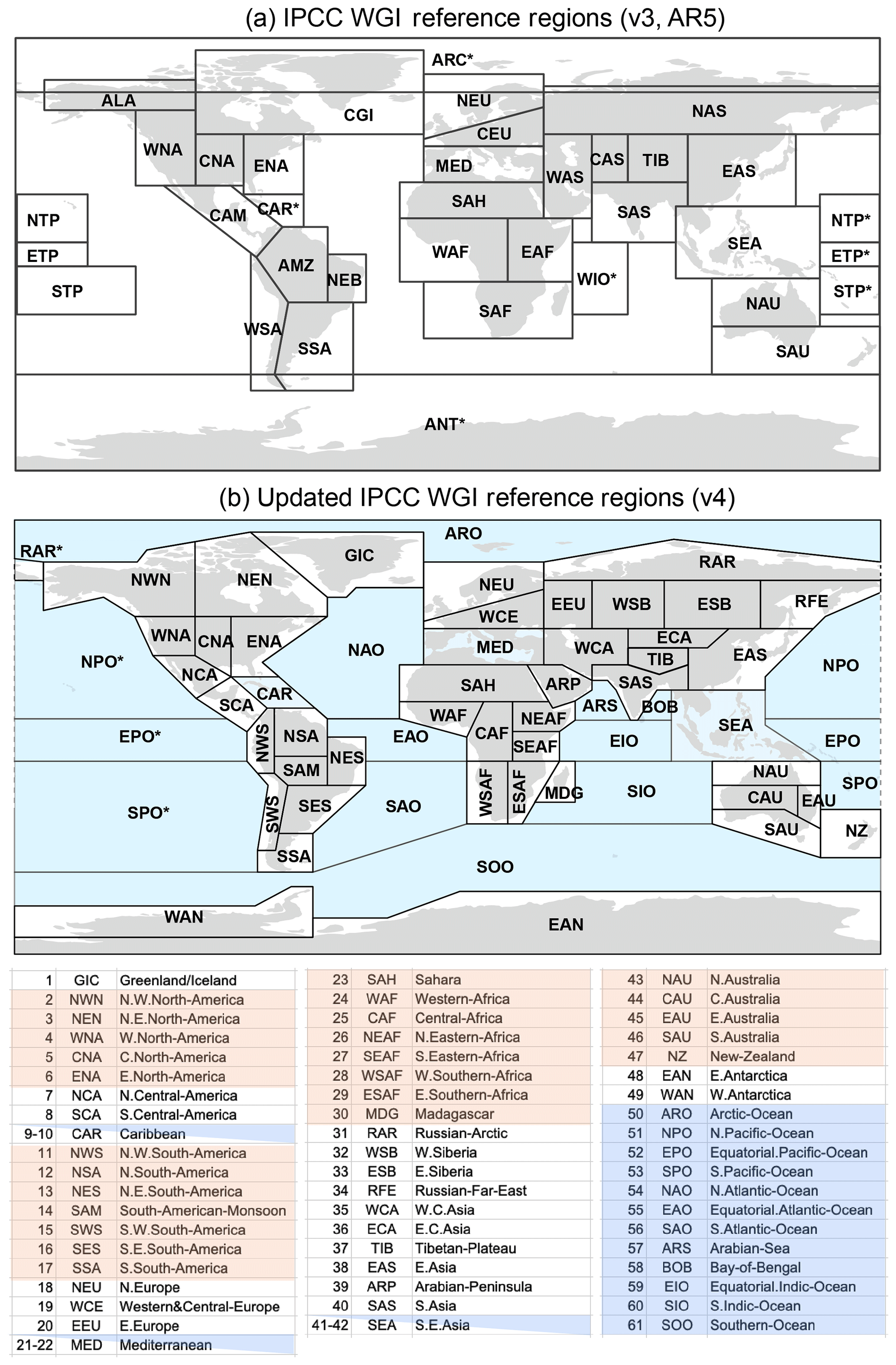
The objective of this work is to expand on existing studies exploring emergence of climate extremes (e.g., Maraun, 2013; Bador et al., 2016; King et al., 2015, 2016; Harrington et al., 2016; Kusunoki et al., 2020; Ossó et al., 2022; Zhang and Gao, 2023; Gampe et al., 2024), by incorporating a wider range of indices, presenting results globally for IPCC reference regions (Iturbide et al., 2020) and using updated model simulations (i.e., the CMIP6 multi-model ensemble), where model weighting is applied to improve both the median estimates for the time of emergence, as well as the associated uncertainty. Specifically, we investigate all 27 core indices developed by the Expert Team in Climate Change Detection and Indices (ETCCDI; e.g., Zhang et al., 2011; Sillmann et al., 2013a; Kim et al., 2020) on annual scales, and 2 ETCCDI indices on seasonal scales. This enables us to capture various characteristics of temperature and precipitation extremes, including their intensity, frequency and duration. With this comprehensive approach, we produce a broad overview across all land regions of how temperature and precipitation extremes change and when and where they may emerge. Our aim is to provide a foundation that will hopefully inspire and motivate further exploration and research into specific indices, regions and mechanisms.

Section 2.1 describes the CMIP6 data set and extreme indices, while the methods for determining time of emergence and model weighting are outlined in Sect. 2.2. We present the results for a selection of indices in Sect. 3 and draw conclusions in Sect. 4. The remaining indices and additional plots can be found in the Supplement.

2 Data and Methods

2.1 Data

To investigate the emergence of climate extremes, we make use of the full range of ETCCDI indices, which illustrate a variety of aspects of surface temperature and precipitation extremes and are straightforward to calculate and interpret (Sillmann et al., 2013a). A detailed description of the 16 indices based on temperature is given in Table A1 and for the 11 indices based on precipitation in Table A2. In a previous project (Sandstad et al., 2022), ETCCDI indices were calculated for historical and future climate simulations from a large number of global climate models that are part of the Coupled Model Intercomparison Project Phase 6 (CMIP6; Eyring et al., 2016). Some ETCCDI indices are percentile-based, and require a base period of time to define a reference climatology (here 1981–2010). The complete dataset of indices used here was subsequently published on the Copernicus Climate Change Services Climate Data Store and is openly available (Sandstad et al., 2022).

For this study, CMIP6 models and ensemble members were selected based on several criteria: data for the complete 1850–2100 time range had to be available (1850–2014 historical, 2015–2100 future) and future simulations had to be available for four emissions scenarios, SSP1-2.6, SSP2-4.5, SSP3-7.0 and SSP5-8.5. Thus, we include a total of 21 distinct models, of which 5 contribute with multiple ensemble members (between 3 and 50). For the remaining models we use only the first member, see Table A3 for details. Throughout this work, we consider only data over land excluding Antarctica.

2.2 Methods

2.2.1 Time of emergence

Our goal is to find the point in time from where the statistical distribution of a particular index deviates significantly and permanently (i.e., until the end of the study period) from the distribution during a reference period (here 1850–1900). This corresponds to the point in time where we can start recognizing changes in climate extremes that exceed natural climate variability, as represented in the climate models (Hawkins and Sutton, 2012). To this end, we use the two-sample Kolmogorov–Smirnov (KS) statistical test, which is non-parametric and compares two empirical distributions based on two independent and identically distributed samples. The KS test checks whether these samples originate from the same underlying distribution, but it does not require any knowledge about the type of the distribution. It also assesses the entire empirical distributions and therefore location, scale and shape, instead of just single moments like mean or variance.

Previous studies using the KS test to determine emergence include Mahlstein et al. (2011, 2012b), King et al. (2015) and Gampe et al. (2024), with notable alternatives being signal-to-noise analyses (e.g., Abatzoglou et al., 2019; Hawkins et al., 2020) or changes in probability ratios (e.g., Harrington et al., 2016; King et al., 2016). We prefer the KS test over other methods, as it does not require any parameter estimation, choice of thresholds or assumptions of normality and is therefore better suited to handle the large and diverse set of indices. Gaetani et al. (2020) found that the KS test lead to more robust ToE results for multi-model ensembles, compared to two signal-to-noise methods.

Several statistical tests similar to the KS test exist; the Cramér–von Mises test, the Anderson–Darling test and Kuiper's test all use different distance measures and are either generally more powerful and/or more sensitive to the tails of the distribution (e.g., Engmann and Cousineau, 2011). However – unlike for the KS test – the distribution of the test statistics is not known for these and has to be approximated via bootstrapping, resulting in high computation times given the size of our data set. Comparing these tests on a small sub-sample did not deliver considerably different results compared to the KS test. Likewise, a permutation test – which only assumes the weaker condition of exchangeability instead of independence – was not feasible to conduct.

The KS test statistic D is defined as

$$\begin{array}{}\text{(1)}& D_{(m,n)}={\text{sup}}_x\left|F_{(\mathrm{1},m)}\left(x\right)-F_{(\mathrm{2},n)}\left(x\right)\right|\end{array}$$

for two empirical distributions F_(1,m)(x) and F_(2,n)(x), with a null hypothesis that both samples are drawn from the same underlying, continuous distribution F(x). This hypothesis is rejected if

$$\begin{array}{}\text{(2)}& D_{(m,n)}>\mathrm{1.358}\cdot \sqrt{(m+n)/(m\cdot n)}\end{array}$$

for a significance level of α=0.05. The distribution F_(1,m)(x) is always based on the reference sample consisting of the 51 yearly index values from 1850 to 1900 at a particular grid point. The sample for the comparison distribution F_(2,n)(x) comprises yearly values in a 20 year rolling time window starting at 1901 and ending with the period 2081–2100 (181 periods in total). For models with multiple ensemble members, the test is performed separately for each member. Grid cells with less than 50 % land cover are discarded. To check the independence requirement, we computed the auto-correlation for a random sub-sample of models and indices (without de-trending them first), which showed no signs of substantial correlation between annual values.

For some indices, ties can per definition occur (e.g., number of consecutive dry days) and the resulting distributions are not necessarily continuous, which can lead to reduced statistical power (Frey, 2020). In these cases, we tested a bootstrap version of the KS test, where p values are determined from a number of sub-samples. This did not result in higher confidence in the test results and used considerably more resources. Likewise, for indices with bounded-support distributions (meaning that all values with non-zero probability fall within a bounded interval, such as for the percentile-based indices TN90p, TN10p, etc.), a variation of the KS test could yield more robust results (Dimitrova et al., 2020), but also requires numerical computation of the critical values, which was not feasible in this study. It was thus decided to proceed with the standard KS test despite its potential limitations.

In Fig. 1, we illustrate how empirical distributions might evolve from the 51 year preindustrial period across 20 year time slices until the year 2100. Shown are histograms of the TXx index (warmest day of the year) for the ACCESS-ESM1.5 model (40 members) and the SSP5-8.5 emissions scenario, averaged over the Northern Europe region. After little change initially, the distributions then shift towards higher temperature values, meaning that there is a substantial change in location. The spread also gradually increases, resulting in a much flatter and broader histogram at the end of the century. For the large majority of ensemble members (85 %), the KS test detects a significant difference (at α=0.05) from the 1981–2000 period onward.

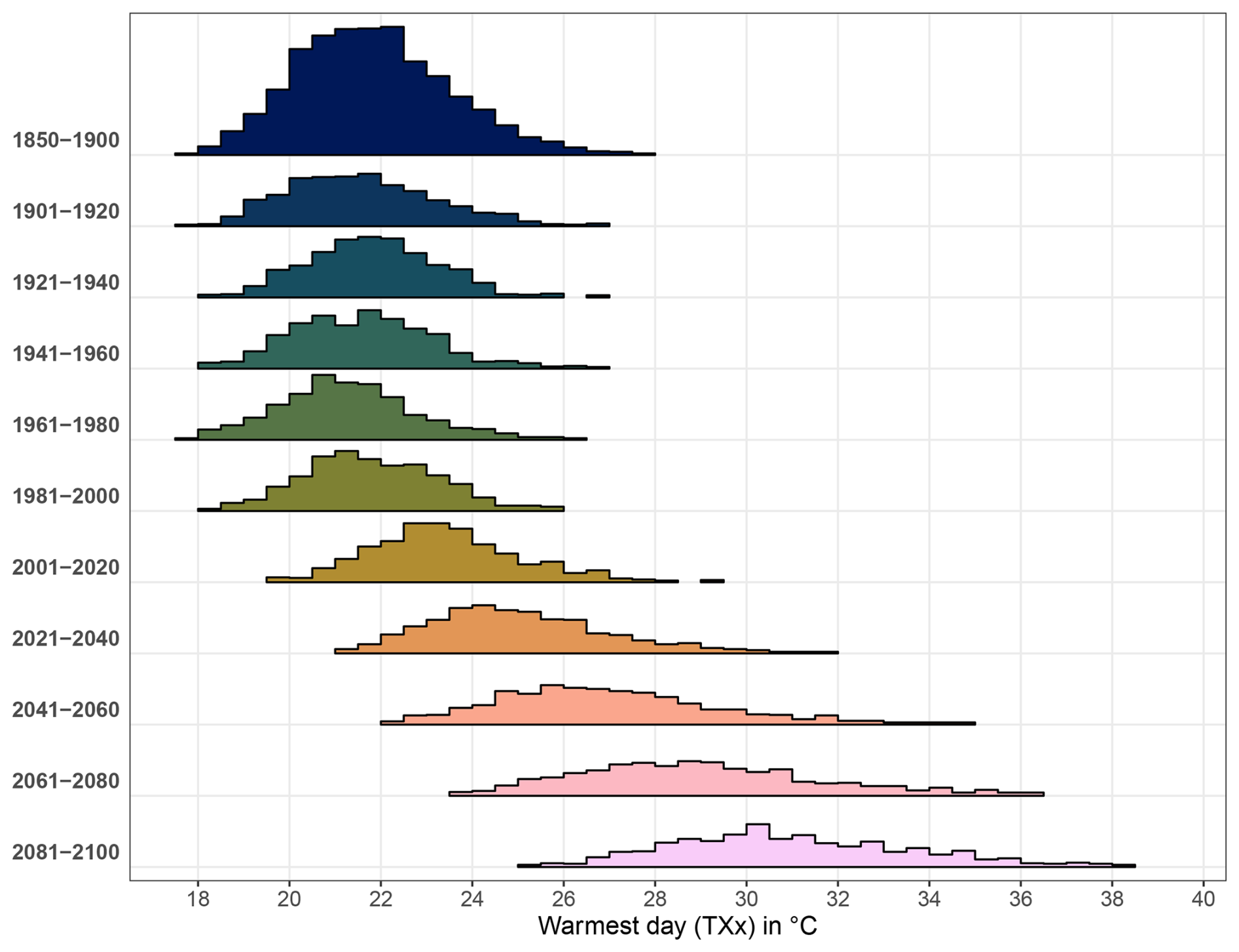
Figure 1 Histograms of TXx values for the SSP5-8.5 scenario from the model ACCESS-ESM1.5, averaged over the Northern Europe region. For illustration purposes, each histogram consists of annual values from all ensemble members. According to the KS test, emergence can first be detected for the 1981–2000 period. We notice a substantial shift towards larger values and an increase in spread from this time period onward.

Once p values from the KS test are established for all time slices at a particular grid point, the time of emergence is computed based on the time series of logical values stating whether a significant deviation between the tested empirical distributions has been found. We use a significance level of α=0.05, but also tested α=0.01, which did not result in considerable differences. The time of emergence is defined as the first period for which the null hypothesis is rejected and for which 95 % of subsequent time periods also show significant difference. This is to balance the (on average) 5 % false positives we can expect and thus a slightly weaker condition than in King et al. (2015), which required all later time periods to be significantly different.

If a time series has not reached emergence until the period starting in 2071, we mark it as not having emerged, as it cannot be reasonably established that any state of emergence will not reverse due to the small number of time periods remaining (cf. Hawkins et al., 2014). For the results, periods are denoted by their first year. Finally, we compute the median time of emergence across IPCC reference regions (Iturbide et al., 2020), and then the weighted median over CMIP6 models as described in the next section.

2.2.2 Model weighting

In this study, we combine results from a large multi-model ensemble to assess the statistical emergence of a new climate in various climate extremes indices. However, combining the outputs from various models is not a problem with a single answer (Knutti, 2010). The most straightforward solution of one model, one vote (i.e., model democracy), though simple to implement, disregards the interdependence between models while simultaneously not taking any overall ensemble bias into account (Knutti et al., 2010). For instance, many models are related through a common development ancestor or origin (Masson and Knutti, 2011; Knutti et al., 2013; Boé, 2018), leading to ideas of institutional rather than model democracy (Leduc et al., 2016). However, model origins may travel, so more automated measures of independence are needed (Pennell and Reichler, 2011).

In recent years, several efforts have been made towards creating better weighting schemes for climate models (e.g., Sanderson et al., 2015a, b, 2017; Knutti et al., 2017; Herger et al., 2018), culminating in a scheme incorporated into the ESMValTool suite (Righi et al., 2020; Andela et al., 2022), which weights both skill and model independence within a given ensemble and for a given variable, where the skill is compared against reanalysis data sets (Brunner et al., 2019, 2020a, b). Alternatively, it is possible to select subsets from a multi-model ensemble, based on similar criteria, for instance as described in Merrifield et al. (2023).

For this work, we have chosen to employ the scheme described in Brunner et al. (2020b) to weight all models comprising the multi-model ensemble. Weights consist of of two components, the first being based on the individual model's past performance for a target variable (here mean temperature or precipitation), compared to ERA5 reanalysis data (Hersbach et al., 2020). The second component measures a model's level of independence from the rest of the ensemble, determined by a clustering of shared biases in climatology of surface air temperature and sea level pressure. Individual members from the same model share an equally distributed model weight among themselves (which is a simple, yet fairly reasonable and transparent solution, although more sophisticated approaches exist; Merrifield et al., 2020). We also weight the target variables precipitation and daily mean temperature separately, to produce two separate sets of weights for the two types of ETCCDI indices. This was done because a good fit to one might not imply a good fit to the other and also because one model (NorESM-LM) had a problem in some of the temperature outputs, so we did not include it at all in the assessment for temperature-based indices. Weights are constant across all grid cells, meaning that potential regional differences in model performance are not considered. Figure 2 shows the weights given to each individual CMIP6 model used in this study. Note that several models receiving a low overall weight (e.g., IPSL-CM6A-LR, both MIROC models for temperature) also receive a low performance weight in Brunner et al. (2020b), while e.g., MPI-ESM1.2-HR and GFDL-ESM4 receive a high performance and overall weight in both studies. The CanESM5 model has a very high equilibrium climate sensitivity (Zelinka et al., 2020) and a large number of ensemble members (50), which together can lead to a multi-model ensemble that is biased towards faster warming if no weighting is applied (Hausfather et al., 2022). CanESM5 receiving a below-average weight, which is then distributed across all ensemble members, likely contributes to generally slightly later times of emergence in the weighted multi-model median, compared to the unweighted one.

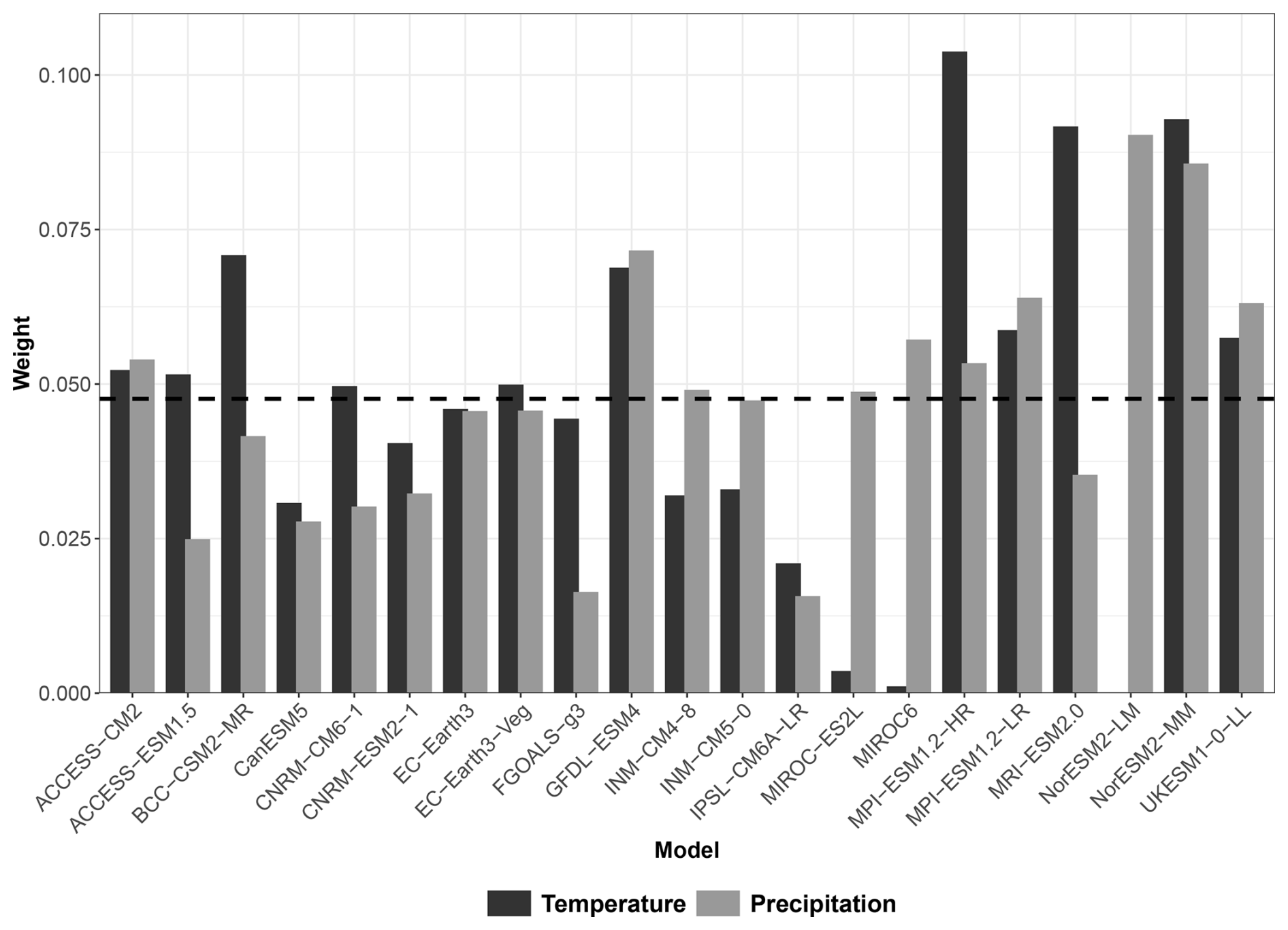
Figure 2 Weights for computing CMIP6 weighted multi-model medians, for temperature- and precipitation-based indices, based on model performance and independence. The dashed line denotes the average weight. Note that the NorESM-LM model is excluded for temperature due to faulty data.

3 Results

In this section, we present results for a subset of the 27 ETCCDI indices, the remaining ones can be found in the Supplement. First, we address annual indices related to surface temperature, then annual indices related to precipitation, and finally a couple of indices on seasonal scales. Although results were computed for four different emissions scenarios (SSP1-2.6, SSP2-4.5, SSP3-7.0 and SSP5-8.5), we opt to only show SSPs 1-2.6 and 5-8.5 in the main article, in order to showcase the widest range of available scenarios. Time of emergence results for SSPs 2-4.5 and 3-7.0 can be found in the Supplement (Sects. S4 and S5).

We show and discuss results for trends of indices to give context and intuition for the emergence, however the trends of extreme indices have been studied in more detail elsewhere, see for instance Sillmann et al. (2013b), IPCC (2021a), Almazroui et al. (2021), Coppola et al. (2021), Li et al. (2021), and Aijur and Al-Ghamdi (2021).

3.1 Annual temperature indices

We first examine a selection of temperature-based indices, comparing in particular maximum versus minimum indices and absolute- versus percentile-based indices.

Figure 3 shows (a) the evolution through time of the global land mean for the “coldest night” index TNn and (b) the spatial patterns of change for the end of century (2071–2100), both relative to 1850–1900, for two contrasting emissions scenarios (SSP1-2.6 and 5-8.5), as well as (c) the time of emergence (ToE). To assess the general level of consensus between all models as to whether or not emergence occurs before 2070, we add hatching to IPCC reference regions¹ (Iturbide et al., 2020) in panel (c) where there is a large degree of disagreement between models, i.e., with either 6–10 models (roughly 25 %–50 %) or 11–14 (roughly 50 %–75 %) out of 20 showing emergence.

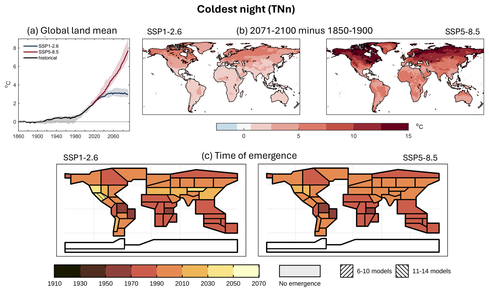
Figure 3 Coldest night (TNn): (a) Time series of global land mean TNn (excluding Antarctica), as a weighted median of all models, each contributing one ensemble member, with corresponding inter-quartile range, for the historical period (1850–2014) and emissions scenarios SSP1-2.6 and SSP5-8.5 (2015–2100), expressed as anomalies relative to the preindustrial period (1850–1900). (b) Difference between end of the 21th century (2071–2100) and preindustrial period (1850–1900) of the weighted multi-model median TNn for SSP1-2.6 and SSP5-8.5, calculated from the same set of simulations. The colorbar is truncated at both end values. (c) TNn time of emergence for IPCC AR6 reference regions and SSP1-2.6/SSP5-8.5 (weighted median of all models and members), referring to the first year of any 20 year time period. Hatched regions indicate low agreement between models as to whether emergence occurs before 2070, with either 6–10 models (roughly 25 %–50 %) or 11–14 (roughly 50 %–75 %) out of 20 showing emergence.

For TNn, we see a strong global warming trend from about the 1980s – while smaller increases can already be seen from 1900 onward (panel a) – which is common to all annual temperature minimum and maximum indices (see Fig. 4a for TNx and Figs. S8a/S9a in the Supplement for TXn/TXx). This warming trend continues for the high emissions scenario SSP5-8.5, but levels off around 2050 in SSP1-2.6. In absolute terms, the largest change in cold night extremes occurs in the northern polar and mid-latitude regions (panel b), with up to 8 °C warming for SSP1-2.6 and up to 15 °C warming for SSP5-8.5 for the weighted multi-model median. The same pattern can be observed for the “coldest day” index TXn in Fig. S8b. The corresponding ToE maps (panel c) indicate, however, that the climate change signal emerges in a much more uniform manner across the globe with many regions in the tropics showing earlier emergence than northern latitudes that have higher warming trends. Most regions show emergence between 1970 and 2010 and only minor differences between scenarios. The latter can be attributed to the fact that the ToE values tend to fall into the historical period of model simulations and there are only a few occurrences in future simulations where the KS test does not show a significant difference. For the Northern Central America region and SSP1-2.6, emergence is only detected after 2030 and only less than 75 % of the models agree that emergence is happening at all. Again, the pattern for the other annual minimum index TXn (Fig. S8c) looks quite similar, although there are some regions in the Americas and the Tibetan Plateau that show no or very late emergence in SSP1-2.6.

Figure 4 Same as Fig. 3, but for warmest night (TNx).

From Figs. 4 and S9 for the annual maximum indices TNx (“warmest night”) and TXx (“warmest day”), we note somewhat different spatial distributions in terms of warming and time of emergence. Here, the difference between the preindustrial period and the end of the 21th century is quite uniform across the globe, up to 3.75 °C warming for SSP1-2.6 and more than 5 °C warming for SSP5-8.5, except for Greenland, which experiences slightly less warming (in the higher emissions scenario; Fig. 4b). Emergence of these indices tends to occur first for the tropics (between 1930 and 1990) and only later for the Southern Hemisphere extratropics (1970–2010) and the Northern Hemisphere extratropics (1990–2010). This is likely due to relatively narrow statistical distributions (i.e., low variability, see Fig. S1 in the Supplement) of these indices in the tropics, where even small changes can be detected as significant by the KS test. As seen before, there are little to no differences between the two scenarios and model agreement is very high.

When comparing annual maximum (TXx/TNx) and minimum (TXn/TNn) indices, we note that, for the northern extratropics and Southern Australia/New Zealand, minimum indices seem to generally emerge at the same time or slightly earlier than maximum indices. On the other hand, the tropical and extratropical regions in southern Africa and South America show emergence up to a couple of decades earlier for annual maximum indices. In some regions (e.g., Eastern Central Asia, Southeastern South America, Western North America), we see that TXx emerges in the recent past for both scenarios, whereas TXn emerges very late or not at all for SSP1-2.6.

Next, we investigate percentile-based indices TN90p (“warm nights”) and TN10p (“cold nights”), which measure the percentage of days per year in the upper/lower decile of the minimum temperature distribution of a given day. These deciles are derived from data in a reference period 1981–2010; figures for the corresponding daytime indices TX90p and TX10p can be found in the Supplement (Figs. S10 and S11). On the global scale, there is a clear increase of warm nights (Fig. 5a), with the increasing trend continuing for SSP5-8.5 and leveling off for SSP1-2.6 after ca. 2040. The percentage of cold nights, on the contrary, decreases over time after a small plateau during 1960–1980 (Fig. 6a). This decreasing trend again continues for the higher emissions scenario and levels off or even slightly reverses for the lower one. We note, however, that the rates of change for the two indices differ greatly in SSP5-8.5. Here, the percentage of warm nights increases up to 60 %–70 % more than in 1850–1900, whereas the percentage of cold nights plateaus at only 15 %–20 % less than in 1850–1900 (likely due to converging towards zero nights); in SSP1-2.6 the change for both remains at ±15 %–20 %. Note that reductions in TN10p greater than 10 % are possible, because we present changes relative to the preindustrial period, which is colder than the 1981–2010 reference period used to define the 10th percentile (the same holds for TX10p).

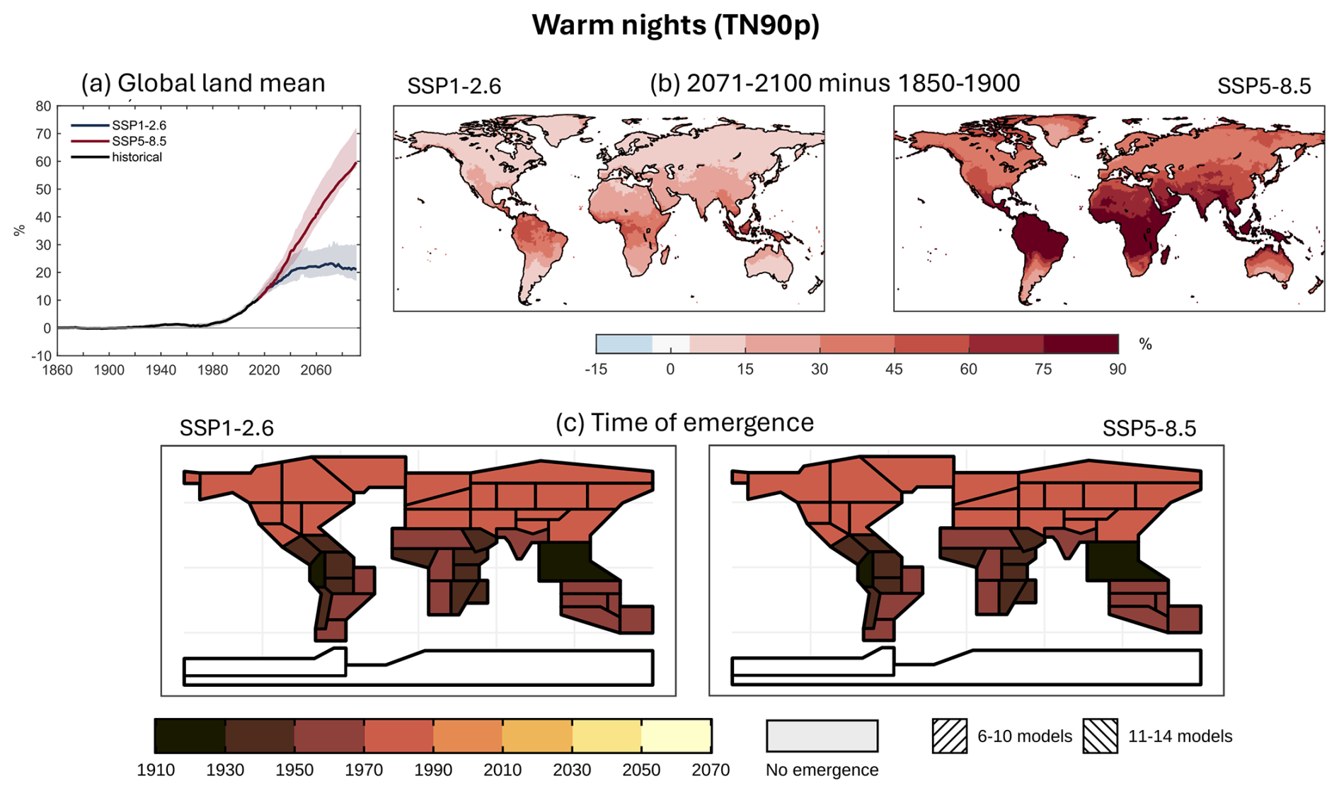
Figure 5 Same as Fig. 3, but for warm nights (TN90p).

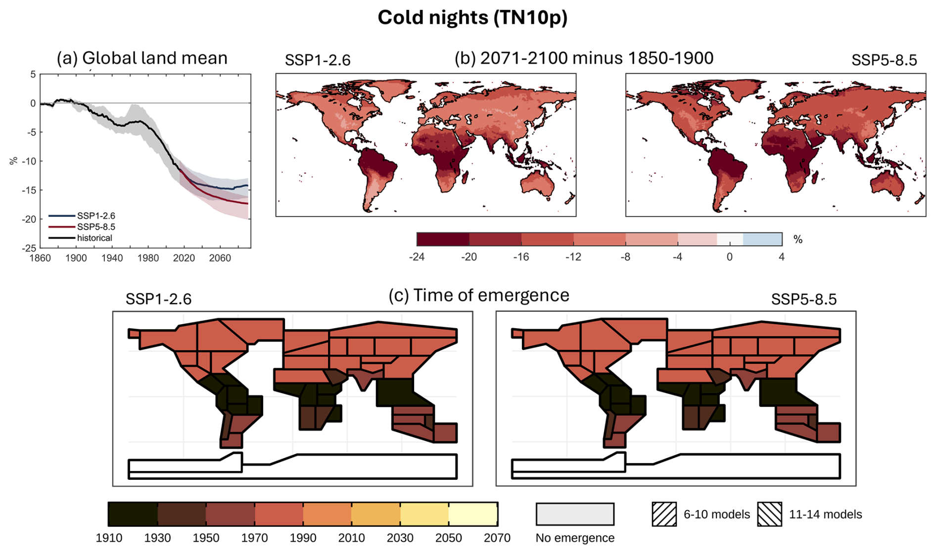
Figure 6 Same as Fig. 3, but for cold nights (TN10p).

This divergence between scenarios for TN90p can also clearly be observed in Fig. 5b, with a stark contrast in terms of absolute change until the end of the 21th century. On the other hand, the corresponding plots for TN10p (Fig. 6b) look quite similar for both SSP1-2.6 and SSP5-8.5, as can be expected from the global timeseries. In all cases, changes in these percentile indices are larger in the tropics than in the extratropics. The ToE patterns (Figs. 5c and 6c) follow these patterns with earlier emergence in the tropics and later emergence in the extratropics.

When comparing results for these percentile-based indices to the absolute temperature indices above, we note that percentile-based indices tend to emerge much earlier, as early as the 1910–1930 period in some tropical regions. The ToE maps for TN10p and TN90p mainly differ in the tropics only, where the former index emerges one time period earlier than the latter in some regions. Northern Hemisphere (NH) extratropics show a uniform emergence during 1970–1990. As all ToEs lie in the historical period of the model simulations, there are no considerable differences between scenarios, for both indices. We observe that in general, nighttime temperature indices emerge either before their daytime equivalents or during the same time period, for both percentile-based and absolute indices.

The “diurnal temperature range” index (DTR; Fig. 7) is the annual mean of the difference between daily maximum and minimum temperatures. Contrary to the previous indices, there is a rather large uncertainty associated with the global land mean, which might be explained by either regional or model differences in the sign of change (cf. Fig. 7b). Overall, DTR values are becoming smaller, as minimum temperatures are increasing faster than maximum temperatures (see also the comparison above). The multi-model median continues on a decreasing trend for SSP5-8.5, while for SSP1-2.6 it stabilizes and reverses quite quickly, beginning at the end of the historical simulations in 2015. However, uncertainty intervals of the two scenarios overlap up until 2100.

Figure 7 Same as Fig. 3, but for diurnal temperature range (DTR).

Figure 7b shows that the sign of the projected change in DTR is mostly negative, as in the global land mean. However, areas like western Europe, the Mediterranean, southern Africa, southern Australia and central America, as well as most of South America, have a strong rising trend in DTR, meaning that, here, daily minimum and maximum temperature tend to diverge. The highest negative change occurs in the Indian subcontinent, the northern high latitudes and central Africa. We note that the two scenarios differ only in the size of change, not the sign, and that changes in DTR – unlike for many other temperature indices – do not seem to depend on latitude. While the maximum change of the global land mean (SSP5-8.5) amounted to −0.7 °C, there are several regions with changes beyond −1 °C at the end of the 21th century, highlighting again the local heterogeneity in the future projections of this index.

Results for ToE in Fig. 7c show that emergence occurs first (as early as the 1970–1990 period) in the NH mid-to-high latitudes and central Africa for both scenarios, and then later in some tropical and subtropical areas in Asia, South America and Oceania, albeit only for the higher emissions scenario and mostly after 2030. For SSP1-2.6, many regions do not show emergence at all. Notably, ToE for the Indian subcontinent falls between 1990 and 2010 for both scenarios, although the absolute change is much larger in SSP5-8.5 by the end of the century. This suggests that even a small deviation from the preindustrial climate was enough to trigger emergence in the recent past. However, it is important to note that early emergence does not mean further climate-induced changes do not occur, in fact they continue to occur and can be even more dramatic in the future. The figure indicates that model agreement is rather low in multiple regions, perhaps most prominently in Eastern Siberia, where the multi-model median ToE lies in the 1970–1990 period, but for SSP1-2.6 less than 75 % of all models agree to emergence happening at all. In Western & Central Europe (ToE 2050–2070 in SSP1-2.6), the multi-model median even overrules the model consensus, as less than 50 % of all models show emergence.

3.2 Annual precipitation indices

While there is a clear global sign of rising temperatures, future changes in precipitation are quite diverse in terms of location and quantity. First, we look at Rx1day (“max 1 d precipitation”), which measures the annual maximum amount of precipitation during a single day. Figure 8a and b again show the change in the global land mean over time and the spatial patterns of the difference between the beginning and end of our time series, respectively. Note that, contrary to the temperature indices and indices related to precipitation frequency, we report the changes for precipitation amount indices as percentages relative to the preindustrial period 1850–1900 (Figs. 8, 10, 12, S17, S20–S22, S25–S27 in the Supplement).

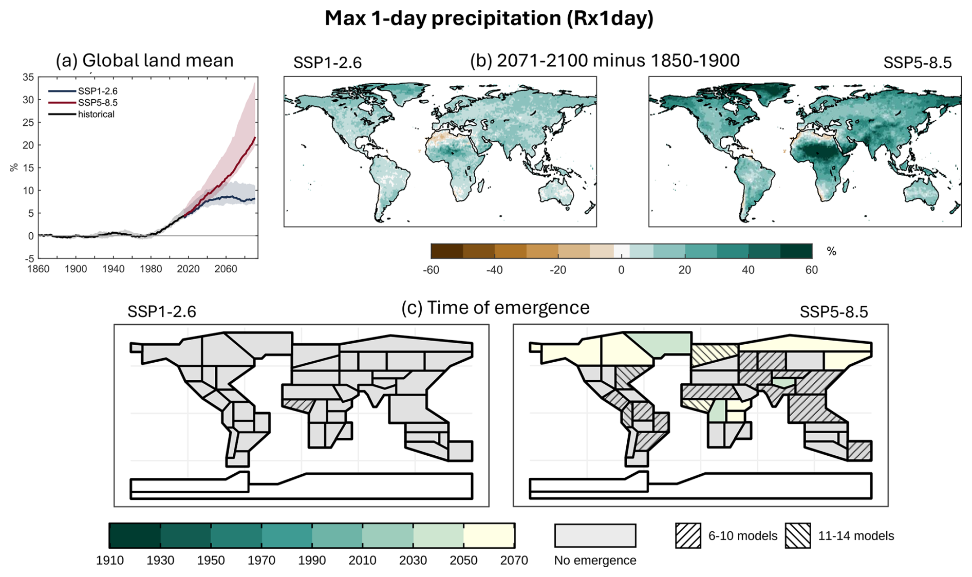
Figure 8 Max 1 d precipitation (Rx1day): (a) Time series of global land mean Rx1day (excluding Antarctica), as a weighted median of all models, each contributing one ensemble member, with corresponding inter-quartile range, for the historical period (1850–2014) and emissions scenarios SSP1-2.6 and SSP5-8.5 (2015–2100), expressed as percentage anomalies relative to the preindustrial period (1850–1900). (b) Difference between end of the 21th century (2071–2100) and preindustrial period (1850–1900) of the weighted multi-model median Rx1day for SSP1-2.6 and SSP5-8.5, calculated from the same set of simulations. The colorbar is truncated at both end values. (c) Rx1day time of emergence for IPCC AR6 reference regions and SSP1-2.6/SSP5-8.5 (weighted median of all models and members), referring to the first year of any 20 year time period. Hatched regions indicate low agreement between models as to whether emergence occurs before 2070, with either 6–10 models (roughly 25 %–50 %) or 11–14 (roughly 50 %–75 %) out of 21 showing emergence.

On the global scale, there is a strong increase in extreme precipitation from the 1980s, which continues as a linear trend for SSP5-8.5 (increasing by more than 20 % by 2100) and flattens out at roughly 8 % for SSP1-2.6 after 2030. We also see that this increase affects most of the globe, with the largest percentage changes of more than 50 % occurring in and a little south of the Sahara, and in northern Greenland (SSP5-8.5). These regions are very dry, meaning small absolute changes give rise to large relative changes. Interestingly, neighboring parts of northern Africa are among the few areas with a slight decrease in Rx1day, mainly for SSP1-2.6. Other small patches with negative sign are found in the Canary Islands, southern Africa and along the Chilean coast. Very similar patterns can be observed for Rx5day (i.e., the total precipitation on the wettest five consecutive days of the year; Fig. S22b).

According to Fig. 8c, only a few regions are projected to experience emergence in the future (i.e., after 2030 and before 2070) and only for the high emissions scenario, namely northern high-latitude regions, central Africa and the Tibetan Plateau. However, there are many regions that do not show emergence for the weighted multi-model median, but nevertheless show high levels of disagreement between models about whether emergence occurs (hatching), which may hint at potential emergence after the end of our data set in 2100. Northern Europe and Western Africa have a multi-model median ToE of 2050–2070, but only up to 75 % of models project emergence. Results for Rx5day in Fig. S22c are similar, with the addition of emergence in Northwestern South America for both scenarios.

The R10mm index (“heavy precipitation days”: Fig. 9) illustrates the number of days per year where more than 10 mm of precipitation fall, which is categorized as the threshold for heavy precipitation. Unlike for Rx1day, there is no continuous rising trend, but rather a decrease until about 1990, followed by a moderate increasing trend for both emissions scenarios. We note that the multi-model medians of the two scenarios seem to split after around 2070, but both have large uncertainty intervals, which in fact almost include zero change at the end of the time series. In Fig. 9b, we see that the sign of change between the end of the 21th century and the preindustrial period differs substantially between regions. Those projected to experience fewer heavy precipitation days compared to the preindustrial era include large parts of South and Central America, southern Africa, the Mediterranean, southeast Asia and Oceania, also mostly containing the small areas with negative Rx1day change seen previously. The highest negative change (>10 fewer heavy precipitation days in SSP5-8.5) is found across the Amazon Basin, Central America and the coast of Chile. In contrast, there is no change around the Sahara and the Arabian Peninsula, supporting the notion that the high percentage changes in Rx1day are related to the historical dry climate of these regions. Most remaining regions experience a small positive change, with larger changes occurring in the Bering Sea coastal areas (>10 more days in SSP5-8.5). Generally, the two scenarios differ in terms of the absolute value of the change only, but not the spatial patterns.

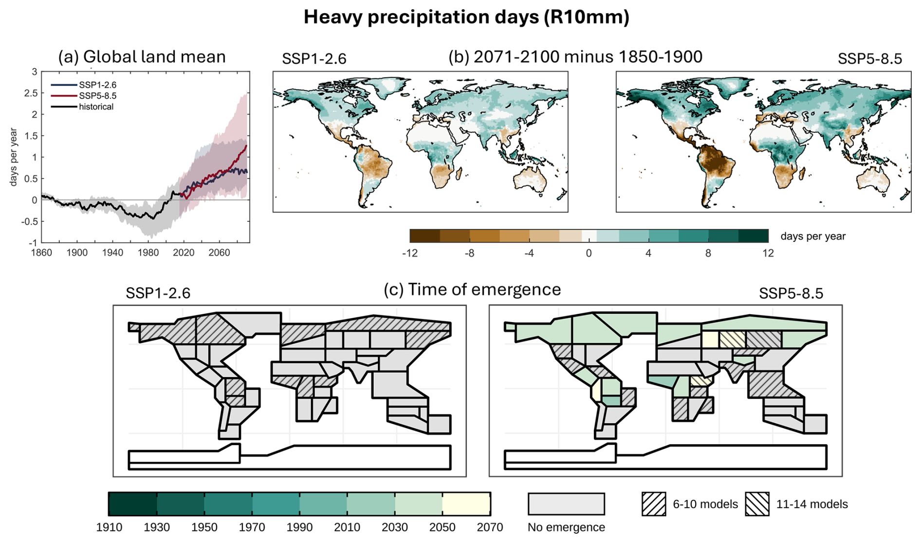
Figure 9 Same as Fig. 8, but for heavy precipitation days (R10mm).

Looking at the ToEs for R10mm (Fig. 9c), we again see no emergence for SSP1-2.6, but a few regions with high model disagreement concerning whether emergence occurs before 2070. In SSP5-8.5, there is emergence for the northern high-latitude regions, central Africa and the Tibetan Plateau (as for Rx1day), but also Central America, matching the area with large absolute changes. The South American Monsoon and Western Africa regions show emergence during the 2010–2030 period, whereas R10mm emerges in the high-latitude regions slightly later during 2030–2050. The decreasing trend in heavy precipitation days for the Mediterranean, Chile, southern Africa, southeast Asia and Oceania does not translate to emergence occurring, at least not before 2070.

When we compare these results with the equivalent indices for heavier and lighter precipitation thresholds, i.e., R20mm and R1mm (the number of days per year with more than 20 or 1 mm precipitation, respectively; Figs. S19 and S18 in the Supplement), both those indices show an overall similar spatial pattern of change to R10mm, but for R20mm the areas of decrease are more constricted, whilst for R1mm they expand. This leads to contrasting signals for the global mean trend: an increase in days for R20mm and R10mm, but a reduction for R1mm (at least in SSP5-8.5), i.e., more days with heavy precipitation, but fewer days with precipitation overall. Time of emergence follows the same overall pattern for all three thresholds, but with later emergence dates in case of R20mm and somewhat earlier in case of R1mm. This pattern of later emergence for indices related to more extreme precipitation also holds true for R99ptot compared to R95ptot (total precipitation on days exceeding the 99th and 95th percentile on wet days, respectively; Figs. S21 and S20), which in turn emerge later than mean precipitation (PRCPTOT, total annual precipitation on wet days; Fig. S17).

Finally, we look at results for the “simple daily intensity index” (SDII; Fig. 10), which measures the average rainfall per day on wet days (i.e., with more or equal to 1 mm). In terms of global land mean trend and spatial distribution of the change between the preindustrial period and the end of the 21th century, there is a strong similarity to the Rx1day index, with most places experiencing an increase in rainfall intensity, including in regions where the overall number of wet days (R1mm) decreases. However, the relative change is larger by a factor of 1.5–2 for Rx1day (maximum 1 d precipitation) compared to SDII (average 1 d precipitation). Despite this similarity, the ToE results for SDII in Fig. 10c differ from the ones for Rx1day in several regions, with earlier timings, and more regions experiencing emergence.

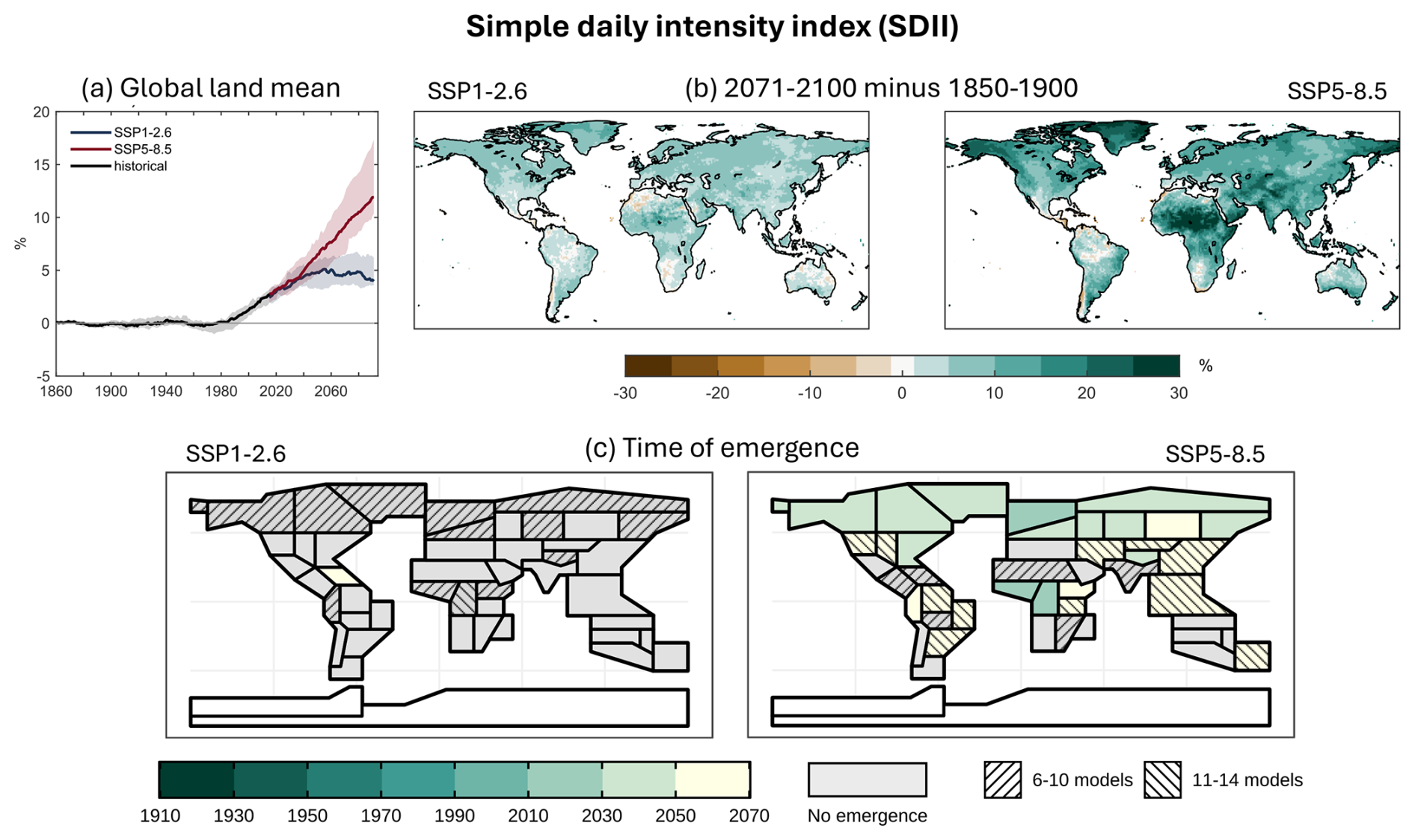
Figure 10 Same as Fig. 8, but for simple daily intensity index (SDII).

In the low emissions scenario, there is emergence only for the Caribbean (although this might be an artifact of very few land points) and signs of model disagreement about whether emergence occurs in several regions. For SSP5-8.5, we see emergence between 2010 and 2050 for Western Africa, the Tibetan Plateau and most regions in the NH extratropics, as well as later emergence for some South American regions, Eastern Asia and Oceania (which were not present for Rx1day). Interestingly, this pattern resembles more the R10mm index in Fig. 9c, but with slightly earlier ToEs. As with most precipitation indices, model uncertainty about whether emergence occurs is generally quite high, apart from regions with emergence before 2050.

3.3 Seasonal indices

In addition to the annual extreme indices, we also investigate seasonal results for a couple of relevant indices, TNn (“coldest night”) and Rx1day (“max 1 d precipitation”). These were chosen for comparison to the annual indices above and related seasonal results in King et al. (2015). Other seasonal indices are also available and might be of particular interest for different regions and applications. Figure 11 shows time series, projected change and ToE results for TNn during June/July/August (JJA). Comparing to Fig. 3a, we see that for SSP5-8.5 the global land mean increases at a lower rate and, at 2100 lies roughly 1.5–2 °C below the annual version. This slower warming appears to be due to the NH extratropics experiencing summertime changes in TNn to a much lower extent (Fig. 11b), which now is in line with other parts of the world, whereas they are warming hotspots in Fig. 3b. Indeed, annual warming of these extremes are dominated by NH winter temperatures, as we can see from the corresponding figure for December/January/February (DJF; Fig. S14 in the Supplement).

The same observation can be made for emergence; while ToEs for DJF largely match the annual results, there are some differences for JJA (Fig. 11c). All regions in the NH extratropics show emergence during the 1990–2010 period for both scenarios – apart from Greenland/Iceland (1970–1990) – whereas annually there is a pattern of later emergence along the west coast of North America in SSP1-2.6. For Western Africa, Northeastern Africa and the Arabian Peninsula, emergence occurs one time period earlier than for annual TNn and DJF. Note also that ToEs for Eastern Central Asia in SSP1-2.6 are much earlier (1990–2010) for JJA than for annual (2030–2050) and DJF (2050–2070).

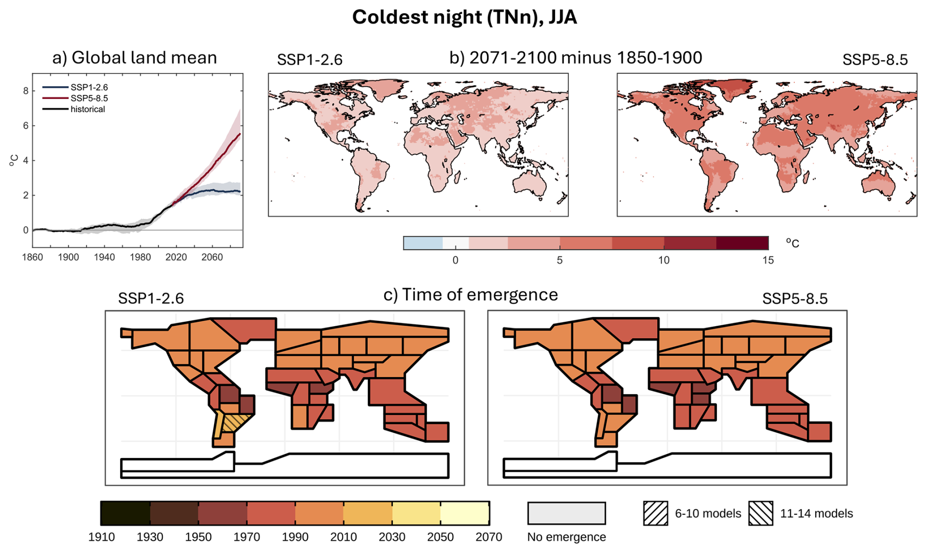
Figure 11 Same as Fig. 3, but for coldest night (TNn) during June/July/August.

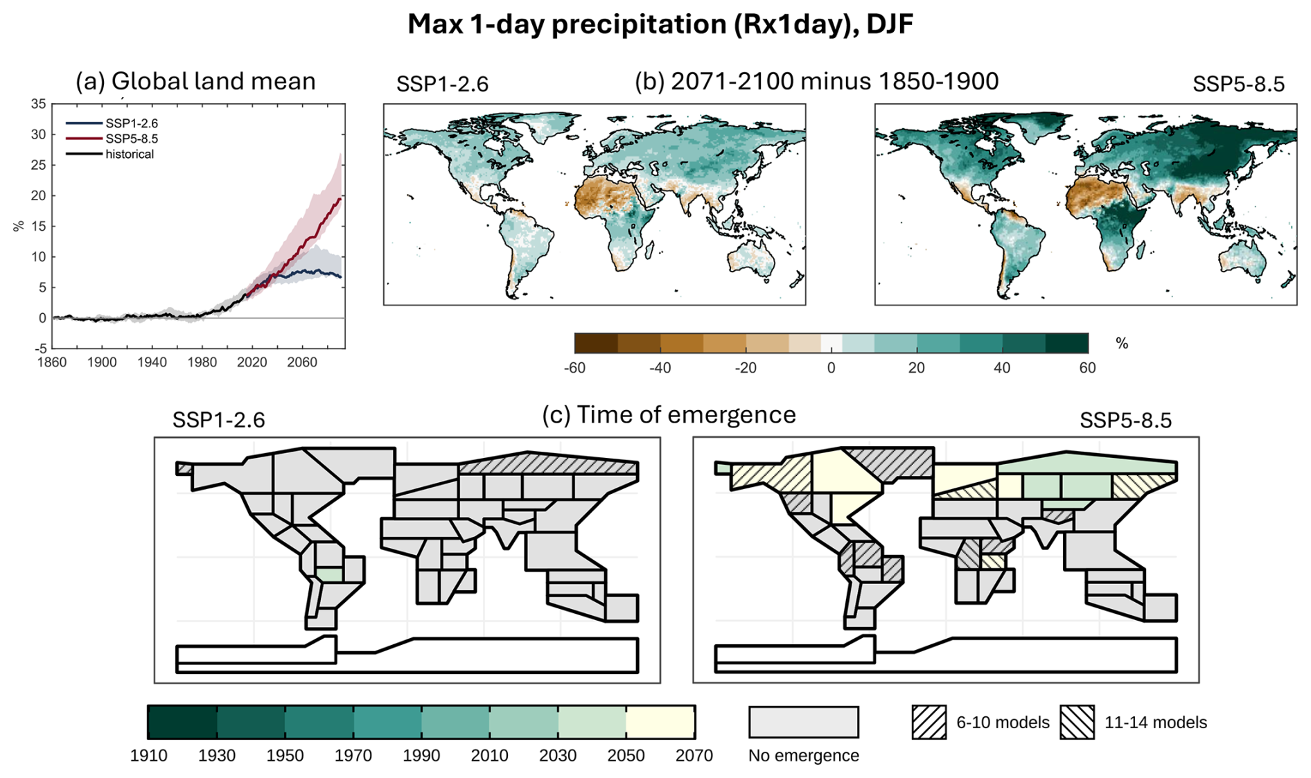
Figure 12 Same as Fig. 8, but for max 1 d precipitation (Rx1day) during December/January/February.

We can also compare these results to Fig. 1e and f in King et al. (2015), which show emergence for TNn in JJA and DJF using projections from CMIP5, the previous generation of global climate models and emissions scenario RCP8.5, also computed using the KS test. In general, ToEs match those from CMIP6, however there is a pattern of later emergence in JJA for southern South America (2000–2040) that is only present for SSP1-2.6 (2010–2030) in our study.

Figure 12 shows Rx1day, maximum 1 d precipitation, for December/January/February. Although the global mean trend is quite similar to the annual index, there are considerable differences in the regional changes (cf., Fig. 8). For DJF, regions with decreases in Rx1day are much larger, including a band across northern Africa, the Indian subcontinent and Central America, where precipitation maxima are expected to be up to 50 % lower than during the preindustrial era. Similarly, the west coasts of southern South America, southern Africa and Australia will see a decrease in seasonal extreme precipitation amounts. The corresponding plot for JJA (Fig. S26b) shows quite a different pattern, with drying areas mostly around the Tropic of Capricorn and Mediterranean/Black Sea/Caspian Sea, and increases in Rx1day elsewhere. The largest percentage increases during DJF occur for large parts of Asia north of the Himalayas, which was not apparent in the annual results, and around the Horn of Africa. For JJA, they mainly lie in the arid regions of the Sahara and the Arabian Peninsula.

Only positive changes in DJF Rx1day seem to lead to emergence (Fig. 12c), indicating that negative changes might be appearing too late in our data set for permanent deviations from preindustrial distributions to be detected and/or that climate variability is very high in these regions. Indeed, emergence only occurs for SSP5-8.5 in mid-to-high latitudes of the NH and for Southeastern Africa, and earliest in the Russian Arctic, Siberia and Eastern Central Asia (2030–2050). DJF is also the only season with emergence in northern and central Europe (see also Figs. S25 and S27 for March/April/May and September/October/November). For JJA, there are only very few regions with ToEs before 2070, namely some tropical regions in South America and Africa, Greenland/Iceland, the Tibetan Plateau and the Arabian Peninsula, but interestingly only for SSP1-2.6, although the changes are much higher in SSP5-8.5.

Comparing with Fig. 1j in King et al. (2015), which shows ToEs for DJF Rx1day, we find that emergence patterns in the NH extratropics and central Africa largely match our results in Fig. 12c, but seem to occur slightly earlier. Figure 1i in King et al. (2015) shows clear signs of emergence for JJA Rx1day in Alaska and Far East Russia (2000–2060), which is not reproduced in our Fig. S26c. However, we find high model disagreement in these regions as to whether emergence occurs. For both seasons, several smaller patches of emergence can be found in King et al. (2015), which in our study are likely too small to change the median across the respective region.

4 Summary and conclusions

In this study, we examined the time of emergence (ToE) of various climate extreme indices (ETCCDI) in the latest generation of climate model simulations (CMIP6) for the IPCC AR6 reference regions, including a weighting of models based on performance and independence. We examined how various aspects of temperature and precipitation extremes change, and when their climate change signal emerges from the noise of climate variability, contrasting a high and a low emissions scenario. We found that most of the temperature indices examined have already emerged in the historical period for the majority of regions, whilst emergence of precipitation-related indices either occurs in the future, or will not occur before the end of our simulations (i.e., by 2070). As such, the latter are also strongly sensitive to the emissions scenario. This later emergence of precipitation indices is consistent with the findings of previous studies such as King et al. (2015), Zhang and Gao (2023) and Gampe et al. (2024). We also found different behaviors for different types of indices within each category (i.e., temperature or precipitation), both in terms of changes over time and ToE.

For instance, annual temperature maxima (TNx and TXx) and minima (TNn and TXn) differ considerably in their spatial patterns of change, but also in their emergence patterns. Annual temperature minima are projected to warm most in the Northern Hemisphere extratropics and yet have a fairly spatially uniform ToE across regions. In contrast, projected warming in annual maxima tends to be more spatially uniform, but emergence occurs around 40 years earlier in the tropics than in the extratropics. Percentile-based indices (TN10p, TX10p, TN90p and TX90p, i.e., number of days per year less than/exceeding the 10th/90th percentile, respectively) tend to emerge considerably earlier than their corresponding absolute indices (i.e., annual maxima/minima) with the earliest ToEs appearing in the tropics – as early as 1910–1930 for TN10p compared to 1970–1990 in the extratropics. Nighttime (i.e., daily minimum) temperature indices generally tend to emerge earlier or at a similar time to daytime (i.e., daily maximum) ones, for both absolute and percentile-based indices. Both of these observations about percentile/absolute and daytime/nighttime indices are in general agreement with results in Zhang and Gao (2023) and Gampe et al. (2024). Although the diurnal temperature range is projected to decrease over large parts of the globe, some regions like the Amazon Basin, the Mediterranean and southern Africa showing an increasing trend. Emergence occurs here towards the end of the historical period in the high northern latitudes and central Africa; elsewhere it occurs either in the future or not at all, depending on the emissions scenario.

Indices relating to precipitation extremes (Rx1day, Rx5day, R99ptot, R95ptot), and also intensity (SDII) are projected to increase in most regions, whilst other indices (R1mm, R10mm, R20mm, PRCPTOT) also show substantial areas of decrease, generally centered on the same regions but with different spatial extents. As to emergence, many indices demonstrate a similar overall spatial pattern, but differ in terms of the actual timing, with later emergence occurring for indices relating to more extreme precipitation, compared to those related to mean precipitation (e.g., contrast Rx1day with PRCPTOT) or lower thresholds (e.g., contrast R20mm/R10mm with R1mm and R99ptot with R95ptot). This general tendency for extreme precipitation to emerge later than mean precipitation is consistent with the findings of Zhang and Gao (2023) and Gampe et al. (2024). The main regions where emergence tends to occur (under the high emissions scenario) includes the high northern latitudes, central Africa and sometimes northern South America (see also Mahlstein et al., 2012b; King et al., 2015). Hints of emergence beyond the end of the 21th century are found in other regions, indicated by high disagreement between models as to whether or not emergence occurs before the end of the simulations. In the lower emissions scenario, there are often no regions or only a few showing any emergence in the multi-model median, but those are sometimes also accompanied by high model disagreement.

We also examined seasonal changes and emergence for TNn, where the spatial pattern of changes for DJF looks very similar to the annual pattern – with the strongest warming in the high northern latitudes – whilst the pattern for JJA is more spatially uniform. Emergence results are similar between the seasons, but somewhat earlier in a few regions for DJF. For Rx1day, the annual index tends to increase in most places, whereas the individual seasons show a decreasing change in several larger regions (in particular DJF and JJA). While only very few regions show emergence for JJA, during DJF emergence mostly occurs in the high northern latitudes, extending over a somewhat wider area than for the annual index. Our results for the seasonal indices largely match those in King et al. (2015), who use a similar method for the previous model generation CMIP5.

There is a range of potential methods to calculate the time of emergence, including statistical tests (such as the KS test used here), signal-to-noise ratios, or changes in probability ratio. The choice of method may affect the exact dates of emergence that we find here, however the KS test has proved through multiple studies to be a versatile and robust way to determine emergence (e.g., Gaetani et al., 2020; King et al., 2015). Other statistical tests (e.g., Anderson–Darling test) are generally more powerful, but were not feasible to apply here due to the amount of computational resources needed. The choice of reference period also affects ToE results, for instance with emergence occurring earlier when using a preindustrial baseline, compared to an end of 20th century baseline as in Zhang and Gao (2023). However, the overall spatial patterns of where emergence first occurs should be consistent.

Our use of a model weighting scheme, taking into account both model interdependence and performance, allows us to avoid the over-representation of closely related models and models that have a large number of ensemble members. Models with a better performance relative to a reanalysis data set are prioritized over ones showing poorer skill. As a consequence, the ToE estimates should be more accurate and robust compared to a simple model consensus.

The IPCC AR6 regions provide a convenient way of summarizing global information across commonly used regions designed to enclose fairly homogeneous areas, both in terms of current climate and projected changes. However, this does hide some regional details, for example along coastlines, which might be expected to experience earlier emergence of temperature indices due to the moderating effect of the ocean on temperature variability (Brunner et al., 2025).

Finally, we note that the scenario dependence for precipitation indices ToEs across many regions shows that reducing emissions has a clear influence on the size of the climate change signal. However, we emphasize that a lack of emergence does not mean that no impact-relevant changes have occurred or will occur, since only large climate change signals can move beyond the noise for places or indices with very high internal variability. Risks from climate change are not only determined by the changes in the probability of a hazard (e.g., in terms of climate extremes and their emergence), but by the exposure and vulnerability of the affected human or ecological system (IPCC, 2023). This is highly context-dependent and adaptation decisions need to be based on local knowledge and sensitivity of the system to the hazard.

In this study, we investigated emergence of climate extremes for 27 different indices and 46 global land regions based on data from 21 climate models and 4 emissions scenarios. While not every individual aspect of these could be explored in detail, our highlighted results connect and strengthen conclusions from previous studies which typically focused on a narrower set of indices or regions. Using a consistent framework involving the Kolmogorov–Smirnov test and a weighted ensemble from the latest model generation CMIP6 enables a systematic comparison across types of extremes, regions and emissions scenarios. Exploitation of these results can help identify avenues for future research, for instance on the physical mechanisms driving changes in extremes, the emergence of specific weather features (e.g., changes in monsoon precipitation), and regionally resolved analyses feeding into actionable impact and risk assessments.

Appendix A: Additional data set information

Tables A1 and A2 contain descriptions and definitions of all 27 ETCCDI indices used in this study, based on Sandstad et al. (2022). Table A3 lists the CMIP6 global climate models and their ensemble members that comprise the multi-model ensemble.

Table A1 ETCCDI indices based on surface temperature, for more detailed descriptions see Sandstad et al. (2022).

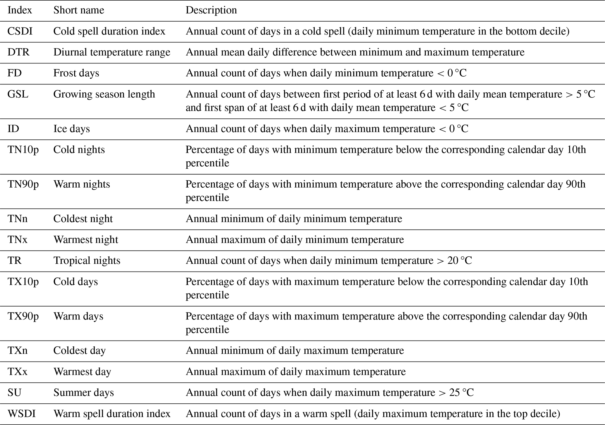
Table A2 ETCCDI indices based on precipitation, for more detailed descriptions see Sandstad et al. (2022).

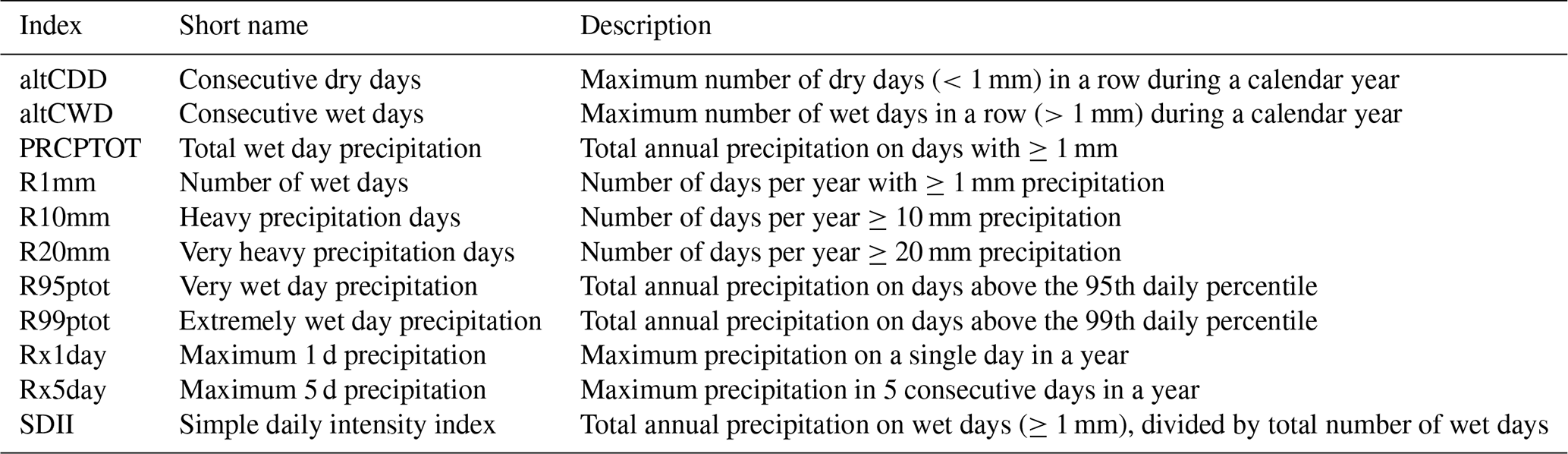
Table A3 Subset of CMIP6 models included in this study and their properties.

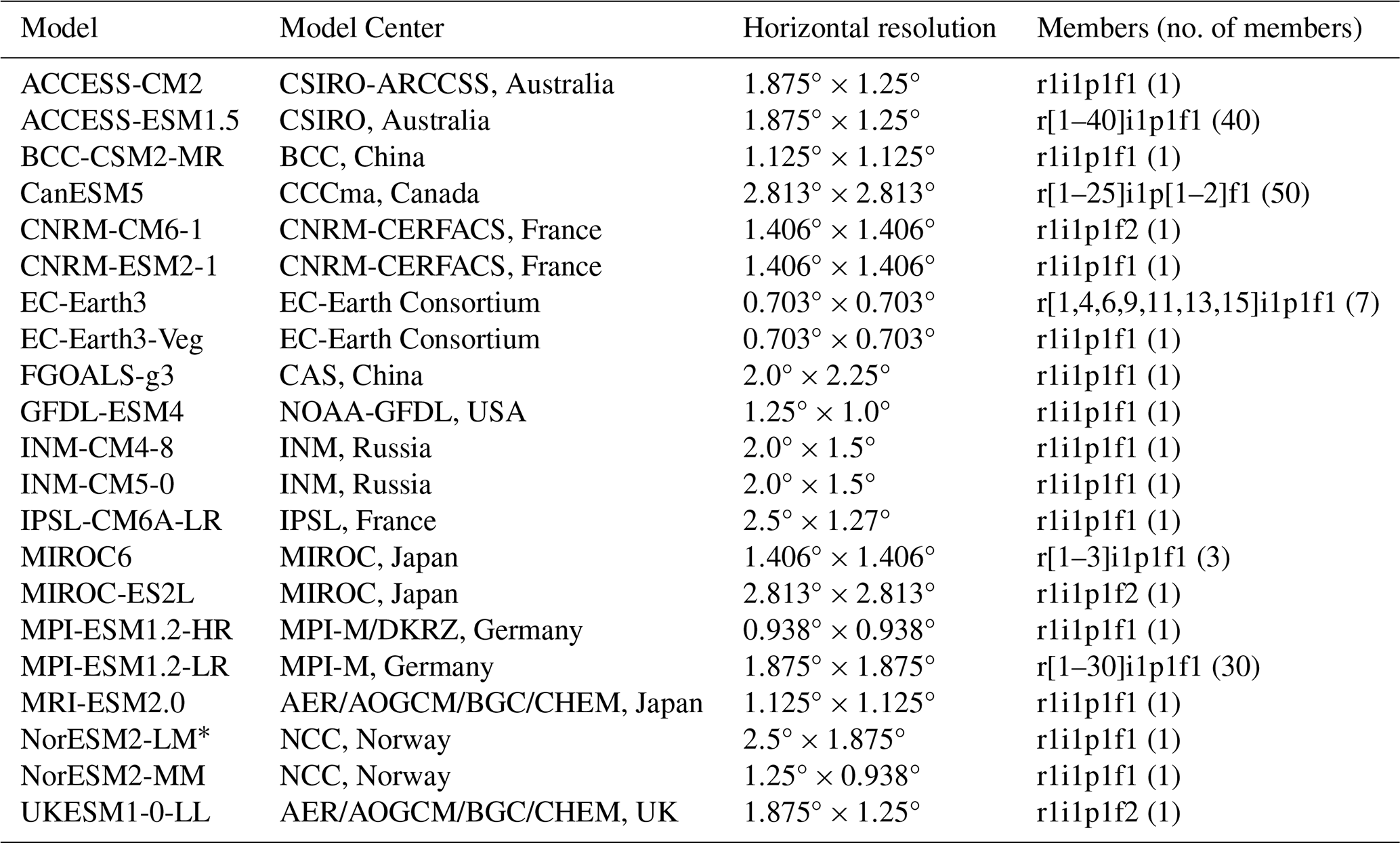
^∗ NorESM2-LM is excluded for temperature indices due to faulty data.