
the Creative Commons Attribution 4.0 License.
the Creative Commons Attribution 4.0 License.
 | 20 Nov 2026
Numerical analysis of dynamics between debris flows and wave propagation using multi-layer shallow water equations
Seungjun Lee
Hyunuk An

Minseok Kim
Taeun Kang
Debris flows are destructive disasters that often cause casualties and property damage, particularly when occurring near residential areas. In reservoir basins, debris flows can reduce effective storage capacity by raising the dead storage level and generate waves that may induce overtopping or structural collapse. Previous numerical studies have applied three-dimensional (3D) hydrodynamics or smoothed particle hydrodynamics to analyze debris flow-induced waves. However, these studies focused on the direct inflow of soil masses into water, without accounting for erosion and entrainment processes. As a result, they have limitations in simulating debris generated in upland areas that undergo erosion and entrainment before entering reservoirs. To address this gap, we developed a one-dimensional (1D) multi-layer simulation model based on shallow water equations that explicitly considers erosion, entrainment, and deposition. The model was validated through theoretical analysis and a laboratory experiment, and applied to the 2020 Sanyang Reservoir collapse event in South Korea. Scenario-based simulations were performed under varying debris flow characteristics and reservoir water levels. The results demonstrate that debris flow momentum strongly correlates with the scale of generated waves, with maximum momentum serving as a reliable predictor of wave magnitude. This study offers a practical framework for assessing debris flow impacts on dam and reservoir safety.
- Article
(10822 KB) - Full-text XML
-
Supplement
(16962 KB) - BibTeX
- EndNote


Debris flows are representative geohazards that occur in both natural and artificial slopes, causing significant changes in the landscape. Generally, landslides refer to ground collapse (Terzaghi, 1950), and debris flows refer to fluid-like movement through the liquefaction of collapsed soil and rock (Takahashi, 1978). Although different factors, such as earthquakes, volcanic activity, heavy rainfall, typhoons, and snow melting trigger debris flow events, rainfall is the most dominant (Wieczorek and Glade, 2005; Kim et al., 2021). When landslides and debris flows occur near residential areas or roads, they cause casualties and property damage and require substantial staffing and resources for recovery. Therefore, most governments focus on developing and implementing disaster prevention and conducting research and development projects in densely populated cities that are prone to disasters. Consequently, several researchers have actively conducted monitoring (Iverson et al., 2011; Zhou et al., 2019), as well as experimental (Hürlimann et al., 2014; Gao et al., 2017; Lyu et al., 2022) and numerical modeling (Denlinger and Iverson, 2001; Pitman et al., 2003; An et al., 2019; Lee et al., 2022a) to analyze debris flows in urban areas. In addition, numerous studies have been conducted based on the above analyses to mitigate damage through structural (Chen et al., 2019; Choi et al., 2021) and non-structural (Zhao et al., 2022) approaches to develop effective response strategies.
However, landslides and debris flows occur in not only urban areas but also mountainous regions with extensive mountain ranges, rivers, and coastal areas. Moreover, areas with large and widespread mountain ranges often have numerous reservoirs and dams, and landslides and debris flows originating from natural slopes in the dam/reservoir basin can affect these structures (Lee et al., 2023). For instance, the landslide and debris flow event on 22 March 1959, in the Pontesei Dam basin resulted in the influx of debris into the reservoir, causing a tsunami and one fatality. Similarly, the landslide and debris flow event in the Vajont Dam basin on 9 October 1963, led to a tsunami that killed nearly 2000 people (Schnitter and Weber, 1964; Slingerland and Voight, 1979). Another example is the landslide and debris flow event on 14 July 2003, in the Three Gorges Reservoir basin, which also generated a tsunami and caused 24 fatalities (Wang et al., 2004). Landslides and debris flows occurring near dams/reservoirs can not only cause performance degradation of the facilities by raising the top of dead storage but also tsunami-type waves by large volumes of sediment flowing into the reservoir (Lee et al., 2023). Therefore, studies on landslides and debris flows in watersheds with dams or reservoirs that are different from those in urban areas are essential for effectively managing dams and reservoirs (ICOLD, 2023). Debris flows occurring not only in dams and reservoirs but also in riverine environments can restrict the flow of rivers or induce eutrophication, thus threatening aquatic ecosystems (Shaffer and Parks, 1994). Similarly, debris flows near the coast can damage economically valuable coastal areas or cause red tide (Kim et al., 2009). Given the multidimensional significance of sediment influx into water systems, sufficient research is essential. However, considering and analyzing the dynamics of two contrasting materials is highly complex, requiring prior research on the impact of debris flow events on a stable hydrological regime. To understand these phenomena, several experiments (Heinrich, 1992; Rzadkiewicz et al., 1997; Heller and Spinneken, 2015; Bullard et al., 2019; de Lange et al., 2020) and numerical analyses have been conducted (Abadie et al., 2010; Pudasaini, 2014; Franci et al., 2020).
Heinrich (1992) and Rzadkiewicz et al. (1997) conducted experiments and numerical analyses on submerged soil collapse. The former assumed that the soil was a rigid body and addressed wave propagation. The latter complemented Heinrich's research by analyzing soil as cohesive sediment instead of a rigid body. Bullard et al. (2019) and de Lange et al. (2020) conducted experiments to analyze the behavior of a wave when debris flows inflow to water along slopes. Bullard et al. (2019) assessed the interaction between debris flow and free water surface, but they used water rather than soil to simulate the debris flow. de Lange et al. (2020) complemented Bullard et al.'s experiment by using soil to simulate the debris flow. However, most of these experiments focused on the behavior of landslides, debris flows, and wave dynamics based on monitoring data. Parallel numerical modeling analysis is necessary to ensure applicability in terms of prediction and response. Accordingly, Pudasaini (2014), Franci et al. (2020), and Guan and Shi (2023) simulated the interaction between debris flow and water using a two-layer technique, three-dimensional (3D) hydrodynamics, and a particle method to analyze this phenomenon physically. Pudasaini (2014) interpreted the phenomenon based on full physical mechanics. However, their simulation results were not validated, and the developed two-layer numerical model was primarily designed for analyzing the liquefaction process of debris flows, i.e., multi-phase. As a result, additional research and improvements are needed to address the interaction mechanisms between debris flows and water. Guan and Shi (2023) used the smoothed particle hydrodynamics (SPH) technique to analyze this phenomenon and validated the accuracy of the simulation results; however, the validation was only performed for specific situations (assuming rigid body behavior of the sediment). In addition, the SPH technique requires further validation due to accuracy variations influenced by the size, shape, and number of particles used in simulations (Han et al., 2019; Su et al., 2025). To achieve comparable simulation accuracy, SPH generally demands greater computational time than grid-based hydrodynamics (Han et al., 2020; Guan and Shi, 2023). Franci et al. (2020) and Franco et al. (2021) simulated soil inflow using the particle finite element method (PFEM) and FLOW-3D, respectively. Although these particle and 3D methods simulate with high accuracy, their high computational requirements pose challenges for field-scale analyses (Ouyang et al., 2013). Therefore, most research on numerical modeling has focused on simulating laboratory experiments. Although some studies address field-scale events, they typically use a mean element size greater than 10 m or a grid resolution exceeding 20 m (Pudasaini, 2014; Franci et al., 2020; Guan and Shi, 2023), which are considered too coarse to accurately analyze debris flow (Stolz and Huggel, 2008). Moreover, existing studies have often overlooked key processes of debris flows, such as erosion, entrainment, and deposition. These processes significantly influence the flow volume and momentum of debris flows (VanDine and Bovis, 2002; Hungr et al., 2005; Iverson et al., 2011; Han et al., 2015; Pudasaini and Krautblatter, 2021; Su et al., 2024), and prior research has demonstrated that the wave magnitude induced by debris flows is directly proportional to their volume and momentum (de Lange et al., 2020; Dai et al., 2023). Therefore, to analyze complex hazards caused by debris flow, it is essential to account for erosion, entrainment, and deposition processes. However, numerical models capable of comprehensively incorporating these processes for analyzing complex hazards remain limited.
Therefore, this study developed a numerical model, that is, a multi-layer flow analysis model based on the hyperbolic form of the shallow water equations, to analyze debris flow events in a dam/reservoir basin (field-scale events). Moreover, the developed numerical model was designed to simulate erosion, entrainment, and deposition processes. The model ensures numerical stability by discretizing it using the finite volume method (FVM). To achieve mathematical and physical stability, the upwinding dispersive correction hydrostatic reconstruction (UDCHR) scheme proposed by Bouchut and Zeitlin (2010) was employed. This paper utilized Voellmy rheology to simulate the debris flow process and validated the performance of the numerical model using the theoretical experiments of Bouchut and Zeitlin (2010) and Krvavica (2020), and laboratory experiment of Rzadkiewicz et al. (1997). Additionally, to examine the model's applicability at a field scale, sensitivity analysis was performed by considering the reservoir collapse event caused by debris flows in Sanyang Reservoir, Icheon, South Korea, in 2020. The sensitivity analysis was conducted by constructing scenarios that incorporated the characteristics of debris flow, such as its rheology parameters, as well as the water level of the reservoir.
The objective of this study is to provide a computationally efficient, process-based framework for the field-scale assessment of debris flow-induced reservoir hazards. Rather than serving as a substitute for fully resolved two-dimensional (2D) or 3D multiphase models, the proposed one-dimensional (1D) multilayer shallow-water model is designed to capture the dominant longitudinal processes of debris flow propagation, erosion–entrainment–deposition, reservoir entry, interfacial momentum transfer, and wave generation. This framework is particularly useful for data-scarce reservoir basins, where repeated scenario analyses are required to evaluate how debris flow characteristics, reservoir water levels, and flow momentum influence wave generation and potential overtopping hazards.
2.1 Numerical modeling
2.1.1 Governing equation
Recently, analysis methods using two-phase or multiphase techniques have been vigorously studied to simulate and analyze debris flow dynamics precisely (Mergili et al., 2020; Shugar et al., 2021). However, further research into the multilayer approach, which explores complex dynamics between distinct systems, such as the interaction between debris flow and water when debris flow enters a water system, is necessary. Studies on multilayer fluid dynamics have included several research efforts to enhance stability and accuracy through mathematical theories (Bouchut and Zeitlin, 2010; Benkhaldoun et al., 2014). However, a practical utilization of the multilayer approach in debris flow analysis is scarce. Therefore, the model developed in this study simulated the debris flow and water using 1D shallow water equations based on the Navier–Stokes equations. Shallow water equations are commonly used to interpret natural fluid phenomena, such as floods and debris flows, where horizontal flow dominates over vertical flow. The phenomenon under investigation in this study also exhibits dominant horizontal flow compared to vertical flow. Therefore, shallow water equations were employed to efficiently simulate this field-scale phenomenon. The hyperbolic conservation form of the mass and momentum balance equation for the debris flow layer is expressed as follows:
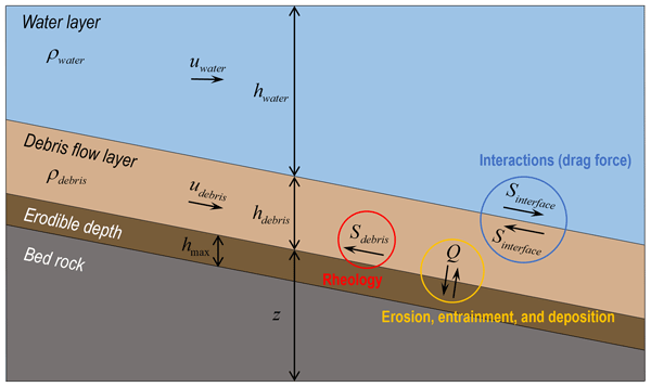
where t denotes time, x is the Cartesian coordinate, j is the layer index, h is the depth of the fluid, u represents the depth-averaged velocity components in the x direction at each layer, g is the acceleration of gravity, ρj is the mass density of the layer j, Q is the term for simulating the erosion-entrainment (Q > 0) and deposition processes (Q < 0), and Sf represents the driving friction in the x direction. The water layer equations are almost the same as those of the debris flow layer. Because the water layer does not have a source term for the mass balance equation, the system has no sink/source. Each layer should be located at the bottom in order of density (Bouchut and Zeitlin, 2010). For example, when analyzing debris flow and water through a bilayer, the debris flows with a relatively high density must be located at a lower position than the water. The overall conceptual framework of the numerical model is illustrated in Fig. 1.
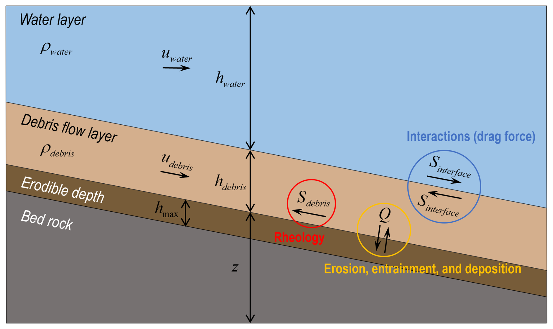
Figure 1Conceptual diagram of the multilayer shallow-water model for debris flow and water-layer interactions.
This study considers the friction between debris flow and water, and Sf, which reflects this, is calculated as follows:
where Sdebris is shear stress for considering the debris flow behaviour; Sinterface is friction between two contact layers; and Smanning is the Manning friction to simulate the momentum transfer process in water propagation, designed to activate only when the debris flow is in dry conditions (hdebris = 0). Thus, in grid cells where water and debris coexist, both Sdebris and Sinterface are applied to the debris flow, while only Sinterface is applied to the water. In grid cells containing only debris flow, only Sdebris is applied, and in cells with only water, Smanning is applied. The shear stress of debris flow is given by the Voellmy rheology as follows (Voellmy, 1955):
where μ and ξ, the Coulomb friction and turbulent friction coefficients, dominate the deceleration behavior when the flow is slow and fast, respectively (Bartelt et al., 2013; Frank et al., 2015). In this study, the mechanism proposed by Canestrelli et al. (2012) was utilized to consider the friction force occurring between debris flow layer and water layer. The mechanism of Sinterface is as follows:
where ρ0 is the mass density of the water; ΔU = U1–U2, while Uk denotes the flow velocity (uk) of the fluid in each layer, and fint is the interface friction coefficient. The mechanism of Manning friction Smanning is as follows:
where n is the Manning's roughness coefficient. This study set Manning's roughness coefficient n as 0.01 based on Arcement and Schneider (1989). Moreover, the algorithm for the three debris flow processes (Q: erosion, entrainment, and deposition rate) proposed by Lee et al. (2022b), which was previously examined through laboratory-scale reproduction and validation by Lim (2021), is as follows:
where is the constant erosion-entrainment rate; is the constant deposition rate; hmax(x,0) is the maximum potential erosion depth; τ is the shear stress of the layer (j); τe and τd are the critical shear stress of erosion and deposition, respectively; is the average potential erosion depth; and s is the channel slope. Notably, this mechanism only affects the debris flow layer not the water layer.
Equation (6), derived from the static equilibrium framework of Medina et al. (2008) and Frank et al. (2015), describes erosion and entrainment when the debris flow shear stress (τ) exceeds τe, and deposition when τ falls below τd. These processes depend on soil depth and can be explained by frictional interactions between the flow and the bed, consistent with Newton's third law. When τ > τe, soil cohesion fails and particles are entrained; when τ < τd, debris flow cohesion fails and material is deposited. Here, τe represents the liquid limit state and τd the transition from solid to liquid. Following Lambe and Whitman (1991) and Boukpeti et al. (2012), τe and τd were set to 1.0 and 0.5 kPa, respectively. While the use of constant erosion, entrainment, and deposition rates may seem idealized, previous work (Lee et al., 2022a) showed that this assumption enhances numerical stability and accuracy compared to variable-rate models without explicit physical constraints.
2.1.2 Spatial and temporal discretization
The governing equation was discretized using FVM. Numerical models that utilize shallow-water governing equations often suffer from an imbalance between the gradient of the water depth and bed slope in irregular topography. This imbalance may cause nonphysical perturbations and instability of the simulation near shocks or wet–dry transitions. Numerous well-balanced numerical schemes have been proposed (e.g. Audusse et al., 2004; Kim et al., 2008; Caleffi and Valiani, 2009). This model implements the hydrostatic reconstruction technique proposed by Audusse et al. (2004), which has been successfully applied to shallow-water models. For stable multilayer simulation and analysis based on shallow water equations, the UDCHR scheme proposed by Bouchut and Zeitlin (2010) was applied. The discretized governing equation for each layer is written as follows:
where Ai is the area of the cell (i); q refers to the state variables such as flow depth and momentum at cell i for the nth time step; Sci is an additional source term to balance the presence of a source; Sfi is the entrainment source term and driving friction term; 𝓙i is an additionally introduced term for the numerical stability of multilayer shallow water system; and Fi is the numerical flux term, which is defined as
where li,p is the length of the cell face p in cell (i) and the subscripts p = {r,l} indicate that the respective value is constructed on the right or left side of the cell, respectively. Notably, the (i) index is used on a uniform template and i ± indicates the cell face on the uniform grid to clearly describe the numerical scheme in a 1D space. Each flux term is calculated as follows:
where ℱ is the numerical flux solver. The interface conserved values are defined as
with the following hydrostatic reconstruction:
where ui,p, hi,p, and zi,p are the reconstructed values for the second-order accuracy at the cell interface p of cell (i) and = , . zj,i is defined as
The source terms are defined as
Additional source terms to ensure balance for the second order scheme are defined as
𝓙 is computed as follows (Bouchut and Zeitlin, 2010):
where 𝒥0 is a term affecting the continuity equation and affects the momentum equation. 𝒥0 is defined as
where θ and κ are calculated as follows:
where (up)+ = and (up)− = ; and in Eq. (19) are defined as
where = when Δz ≥ 0 and = when Δz ≤ 0 and Δz is the difference between the contacted cells, calculated as zi,r–. in Eq. (16) is defined as
where 𝒥1 is calculated as 𝒥1 = and δp is defined as
The numerical fluxes in Eq. (8) are calculated using the Harten–Lax–van Leer contact approximate Riemann solver in the developed model. Therefore, the conservative values over the time step Δt are calculated as follows:
The additional source/sink terms for entrainment and driving friction force are written as
The inclusion of a friction term can cause numerical instability within a discretized domain, particularly when a dry–wet transition exists (An et al., 2019). In other words, if the flow depth approaches zero, driving friction can result in an exaggerated force, which reverses the flow in a non-physical manner. Therefore, the friction term should be properly treated. The developed model implements an implicit discretization based on the splitting method (Liang and Marche, 2009), which is equivalent to solving the following equation:
The Euler implicit discretization of the above equation yields the following:
The right side of Eq. (27) can be represented by the Taylor series expansion as
where Δq = . Ignoring high-order terms and substituting Eq. (28) into Eq. (27) yields
where
where I is a unit matrix and
Equation (31) ignores the effects of off-diagonal entries. This method can be successfully applied to shallow water systems with Manning friction (An and Yu, 2014). Denoting = yields the implicit scheme written as
Although the friction terms are implicitly discretized, the friction force in Eq. (32) can cause exaggerated reverse flow, which is physically implausible (An et al., 2019). Therefore, if the driving friction results in reverse flow, the fluid flow stops. The time step Δt is determined in each step based on convergence by the Courant–Friedrichs–Lewy condition as follows:
where C, a dimensionless number called the Courant number, was set as 0.5 in this study. This study utilized the experimental results of Bouchut and Zeitlin (2010), Krvavica (2020), and Rzadkiewicz et al. (1997) to validate the model performance. The validation is described in the following subsection.
2.2 Validations
In this section, the model developed in this study is validated. First, this study conducted fundamental numerical validations based on three theoretical experiments of Bouchut and Zeitlin (2010) and Krvavica (2020). Moreover, to validate the performance in real situations the numerical model developed in this study is validated in the submarine debris flow and wave generation against the experimental tests of Rzadkiewicz et al. (1997).
2.2.1 Theoretical experiments
It is essential not only to perform tests in experiments and field events but also to test numerical performance at the mathematical and programming levels to utilize the developed numerical model. This study used the three validation cases in Bouchut and Zeitlin (2010) and Krvavica (2020).
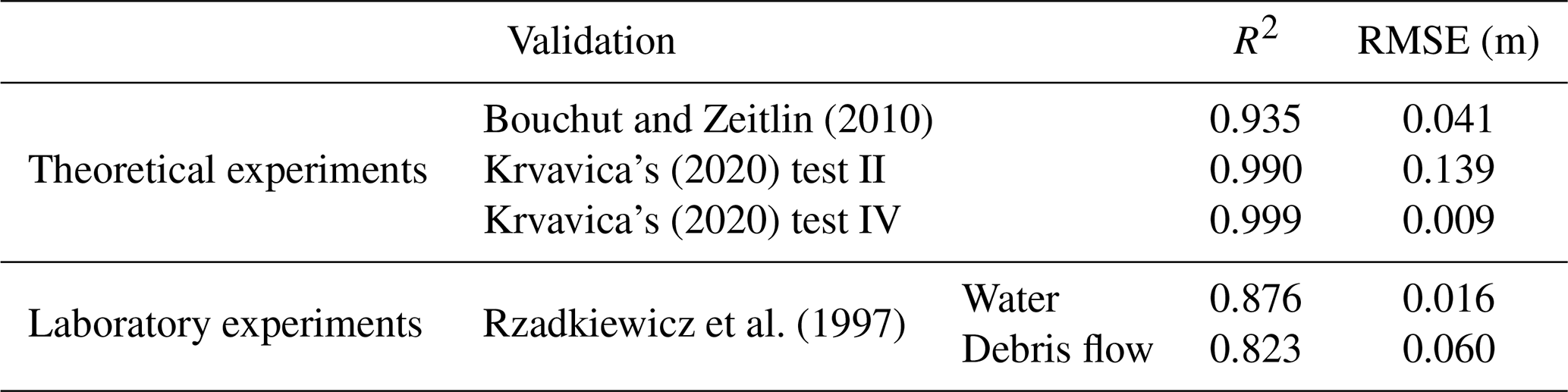
The validation results in Fig. 2 show that light blue represents the upper layer, dark blue depicts the lower layer, and the black solid line signifies the analytical solution for the lower or upper layer. Figure 2a is a case in Bouchut and Zeitlin (2010), where the density of the upper layer is 0.95 times that of the lower layer, with the simulation at 0.5 s later depicted in Fig. 2d. Figure 2b, Test II: an internal collision of two dam breaks from Krvavica (2020), shows a condition where the density of the upper layer is 0.98 times that of the lower layer, with the state 25 s later shown in Fig. 2e. Figure 2c corresponds to Test IV: an internal dam break from Krvavica (2020), where the upper layer's density is 0.4 times that of the lower layer, and the simulation 5 s later is shown in Fig. 2f. As demonstrated in Fig. 2 and Table 1, the performance of numerical model developed in this study has been confirmed to be well-constructed both mathematically and programmatically.
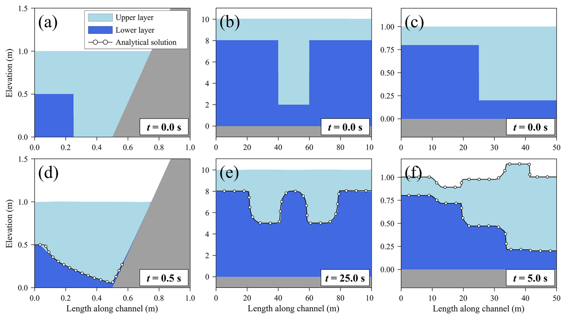
Figure 2Numerical tests: (a, d) Bouchut and Zeitlin (2010), (b, e) Krvavica's (2020) Test II and (c, f) Krvavica's (2020) Test IV.
Table 1Quantitative validation results of the proposed numerical model against theoretical and laboratory benchmark tests.
2.2.2 Laboratory experiment: subaqueous debris flow
Rzadkiewicz et al. (1997) experimented with the subaqueous soil slope failure scenario, as shown in Fig. 3a, and they set a debris density of 1950 kg m−3 and a water density of 1000 kg m−3. Rzadkiewicz et al. (1997) presented experimental results on water surface and debris flow behavior at 0.4 and 0.8 s, as depicted in Fig. 4, respectively.
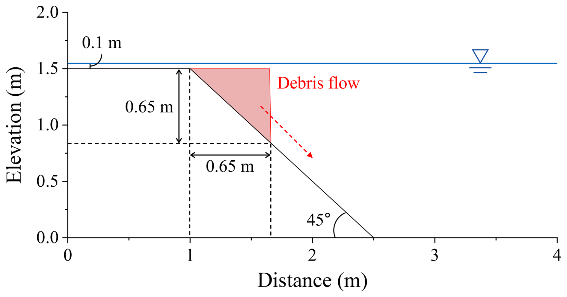
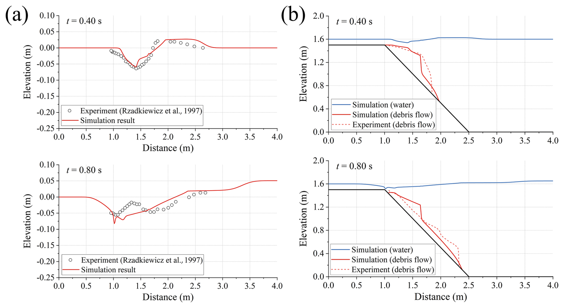
Figure 4Comparison between the simulated and Rzadkiewicz et al.'s (1997) experimental waves at 0.40 and 0.80 s: (a) water surface and (b) combined water surface and debris flow thickness.
Figure 4a reveals the reproducibility of water levels, where the plotted dots represent the observed values from Rzadkiewicz et al. (1997), and the solid red line indicates the simulation results from this study. Figure 4b presents the overall simulation results, focusing on the reproducibility of debris flow. In this figure, the blue solid line represents water levels, the red solid line represents debris flow, the black solid line represents topography, and the red dotted line corresponds to the debris flow thickness observed in Rzadkiewicz et al. (1997). In this study, to simulate the experiment of Rzadkiewicz et al. (1997), the parameters of Voellmy rheology and the interface friction coefficient were calibrated to μ = 0.15, ξ = 50 m s−2, and fint = 10.0, respectively. The three parameters were calibrated through back-analysis, but their values were set within the range presented and suggested in previous studies. In this context, the value of ξ is significantly lower than those used in previous studies (e.g. Cesca and D'Agostino, 2008; Frank et al., 2015), while fint is notably higher (Canestrelli et al., 2012). In this study, μ was estimated to be higher and ξ lower than in previous works, which may be due to the debris flow being generated and propagating under submerged conditions, thereby experiencing higher overall pressure and additional resistance from water. Conversely, the larger value of fint is likely related to the debris-dominated nature of the flow, where comparable volumes of sediment and water interact, unlike in water-dominated flows observed in earlier studies. This explanation is conceptual, and further sensitivity analysis will be required to verify these findings. However, since these values do not deviate substantially from the range used in prior research, they have been assessed as reasonable.
At 0.4 s, the simulation results aligned well with the experimental observations, accurately capturing the water level reduction around 1.5 m. At 0.8 s, the simulation also exhibited good agreement with the experimental data, particularly in reproducing the water level patterns. However, the simulation failed to capture the fine oscillations of the water level. This phenomenon is believed to occur due to the abrupt collapse of sediment along the slope. In areas where the sediment layer becomes thinner (around 1.0–1.5 m), negative pressure is exerted on the water, whereas in areas where the sediment layer thickens (around 1.5–2.0 m), positive pressure is exerted. A hydraulic jump-like appears at the intersection of these negative and positive pressures, near 1.5 m – where the water layer thickens rapidly – drawing water toward the negative pressure region. It has been identified that the numerical model developed in this study has limitations in accurately simulating this phenomenon. Nevertheless, comparing the simulated results with experimental observations reveals that while the reproduction of microscopic details was somewhat limited due to the depth-averaged shallow water modeling characteristics, the model demonstrated satisfactory accuracy in macroscopic aspects such as wave height and propagation velocity. R2 and RMSE (Root Mean Square Error) analysis was conducted to validate the accuracy of the simulation results (Table 1). The R2 for the water surface oscillation and debris flow thickness were 0.876 and 0.823, respectively. The RMSE values for these results were 0.016 and 0.060 m, respectively, indicating low discrepancies between the simulation results and experimental observations. The model developed in this study successfully simulated three theoretical experiments and the laboratory experiment. This study analyzed the wave caused by debris flows occurring at the field scale based on a hypothetical method using our model. The following section discusses this in detail.
3.1 Study area and event
This study conducted a two-layer dynamic flow analysis for Sanyang Reservoir in Icheon, Gyeonggi, South Korea. The Korea Rural Community Corporation (KRC) designed and constructed it in 1966, and it is managed by Icheon City. According to the KRC, the reservoir is a small-scale agricultural reservoir with an earthen dam 9.5 m high and 126 m long. It has been in operation for over 50 years, making it an aging reservoir (Fig. 5). Sanyang Reservoir has a catchment area of 192 ha, a surface area of 2.8 ha, and an effective storage capacity of 60 000 tons and serves as a water storage facility for agricultural purposes (https://rawris.ekr.or.kr/main.do, last access: 18 February 2023).
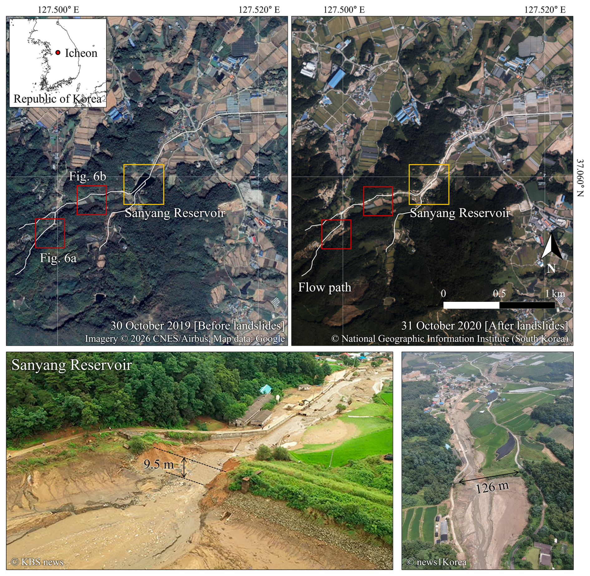
Figure 5Study area and impacts of the 2020 Sanyang Reservoir collapse event in Icheon, South Korea. Pre-event satellite imagery: Imagery © 2026 CNES/Airbus, Map data © Google (Google Earth). Post-event aerial imagery: © National Geographic Information Institute (NGII), Republic of Korea. Field photographs: © KBS News and © News1 Korea.
Despite receiving a “satisfactory” safety rating in the first half of 2020 from the KRC's reservoir safety assessment, the Sanyang Reservoir collapsed due to concentrated heavy rainfall of 193 mm (7 h)−1 on 2 August 2020, between 00:00 and 07:00 Korea Standard Time (KST, UTC+9). The collapse reportedly occurred at 07:30 KST. Although no casualties were reported, approximately 10 houses were flooded, and 6 ha of fields and rice paddies were inundated, resulting in significant property damage (Fig. 5).
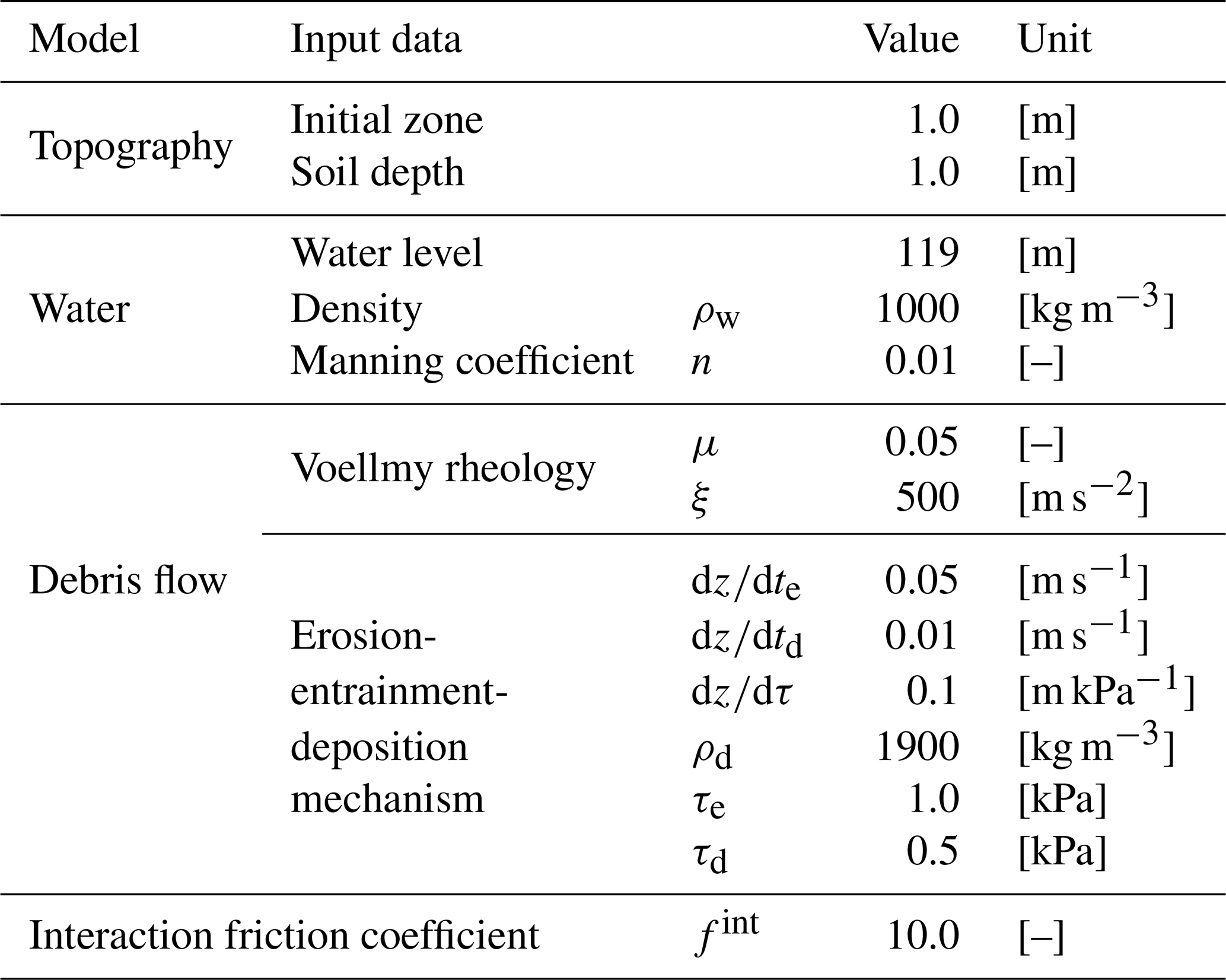
According to the National Geographic Information Institute of Korea (NGII), the study area is widely covered with sandy loam and silty clay loam soils, with soil depths ranging from 0.5 to 2.0 m and an average depth of approximately 1.0 m. In addition, geological survey data from the Korea Institute of Geoscience and Mineral Resources indicate that the area is predominantly underlain by Precambrian banded biotite gneiss, with minor distributions of Jurassic granitic rocks and Quaternary alluvial deposits nearby. Based on these conditions, a soil depth of 1.0 m was adopted for debris flow analysis in this study, and the failure depth was also set to 1.0 m (Table 2).
Table 2Input data and parameters setting for numerical models used in this study.
The explicit cause of the dam collapse has not been investigated and reported. However, satellite images before and after the incident, as shown in Fig. 6, yield evidence of debris flows. Figure 6a and b show pre- and post-event satellite images of the areas marked in Fig. 5. According to news and media, numerous landslides and debris flow events occurred in Icheon City during the same period. Therefore, this study assumed that external rather than internal factors were behind the reservoir collapse. In this context, the external factors are assumed to be landslides and debris flow, based on Fig. 5 and news reports.
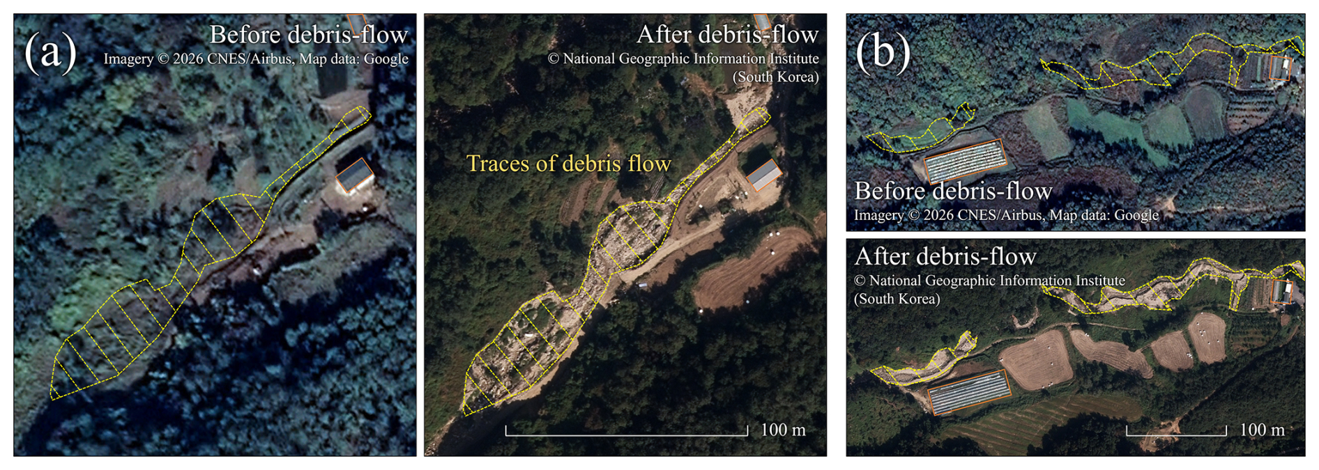
Figure 6Evidence of debris-flow occurrence at two locations marked in Fig. 5. Panels (a) and (b) each show pre- and post-event imagery of one location. Pre-event imagery: Imagery © 2026 CNES/Airbus, Map data © Google (Google Earth). Post-event imagery: © National Geographic Information Institute (NGII), Republic of Korea.
This reservoir has a history of collapse, which occurred in 1970, and the recent incident marks the second collapse. Therefore, this facility had a risk of future collapse. Consequently, numerical modeling is imperative for efficient operation and the development of stable countermeasures for such regions. This study utilized the developed model to simulate and analyze the phenomenon of sediment inflow in Sanyang Reservoir. However, we could not determine the reservoir water level at the time of the collapse due to inadequate field data for the incident period. Therefore, this study assumed that the reservoir water level at the time of the incident was at the flood level (119 m), considering that the incident occurred during the flood season (21 June–20 September; as established by the Ministry of Government Legislation in South Korea).
The input data used for the analysis are shown in Fig. 7. The topographic data utilized a 5 m × 5 m resolution digital elevation model (DEM) provided by the NGII (Fig. 7a). As the model used in this study is a 1D analysis, it requires the establishment of flow paths for debris flow. Therefore, this study calculated the flow paths of the basin, depicted by the red solid line in Fig. 7a. The traces of debris flow observed in Figs. 5 and 6 suggest that the debris flow entered the reservoir from flow path 2. Figure 7b illustrates the longitudinal section of the flow path 2, and Fig. 7c depicts the topography near the reservoir.
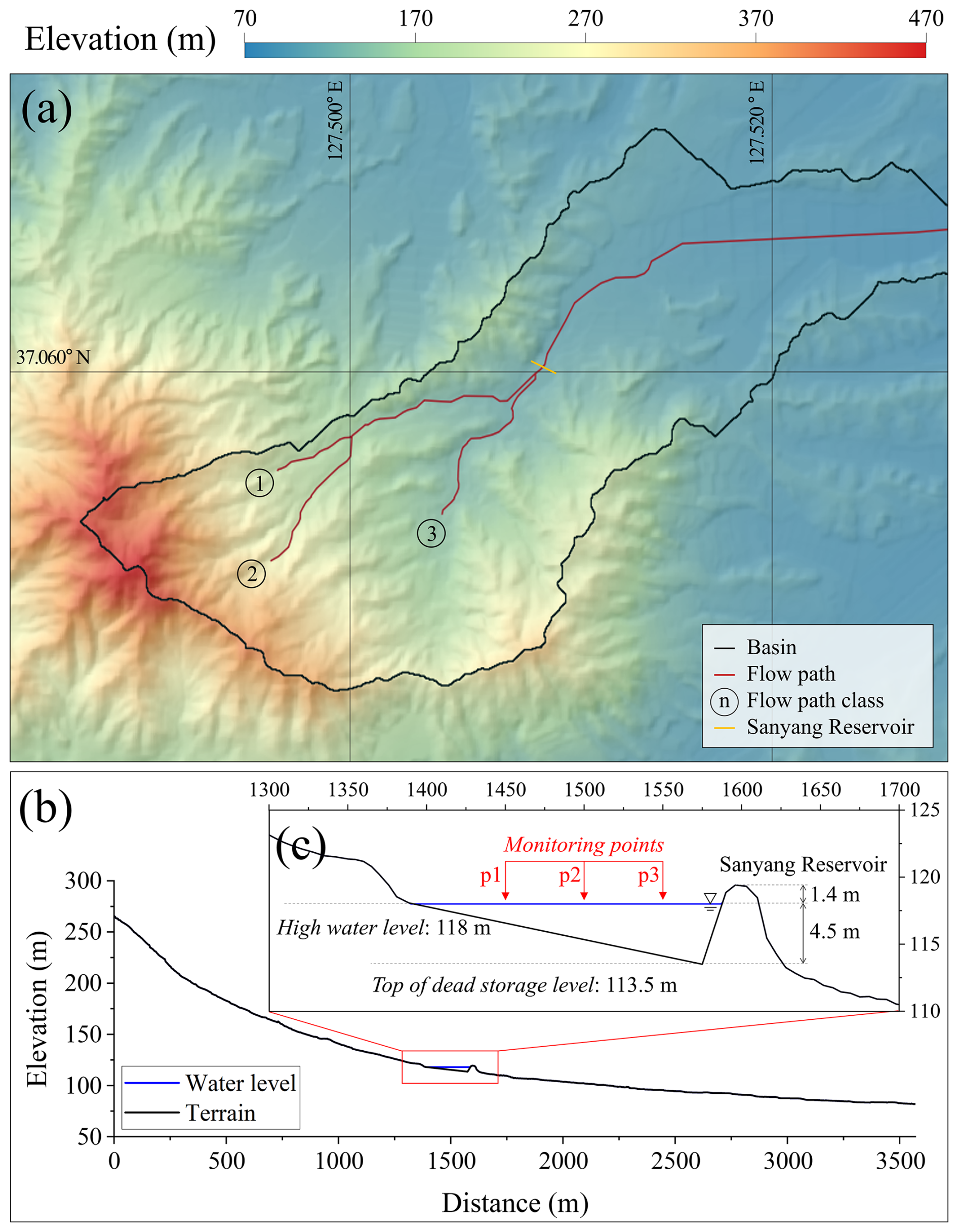
Figure 7Topography data of Sanyang Reservoir basin: (a) digital elevation model (DEM); (b) longitudinal section of the flow path 2; and (c) longitudinal section near the Sanyang Reservoir. The DEM was generated from 1:5000-scale digital topographic maps provided by the National Geographic Information Institute (NGII), Republic of Korea.
This study assumed that the internal topography of the reservoir is linear based on the reservoir information. Reservoir water level fluctuations by debris flow were observed at points p1, p2, and p3, as marked with red arrows in Fig. 7c.
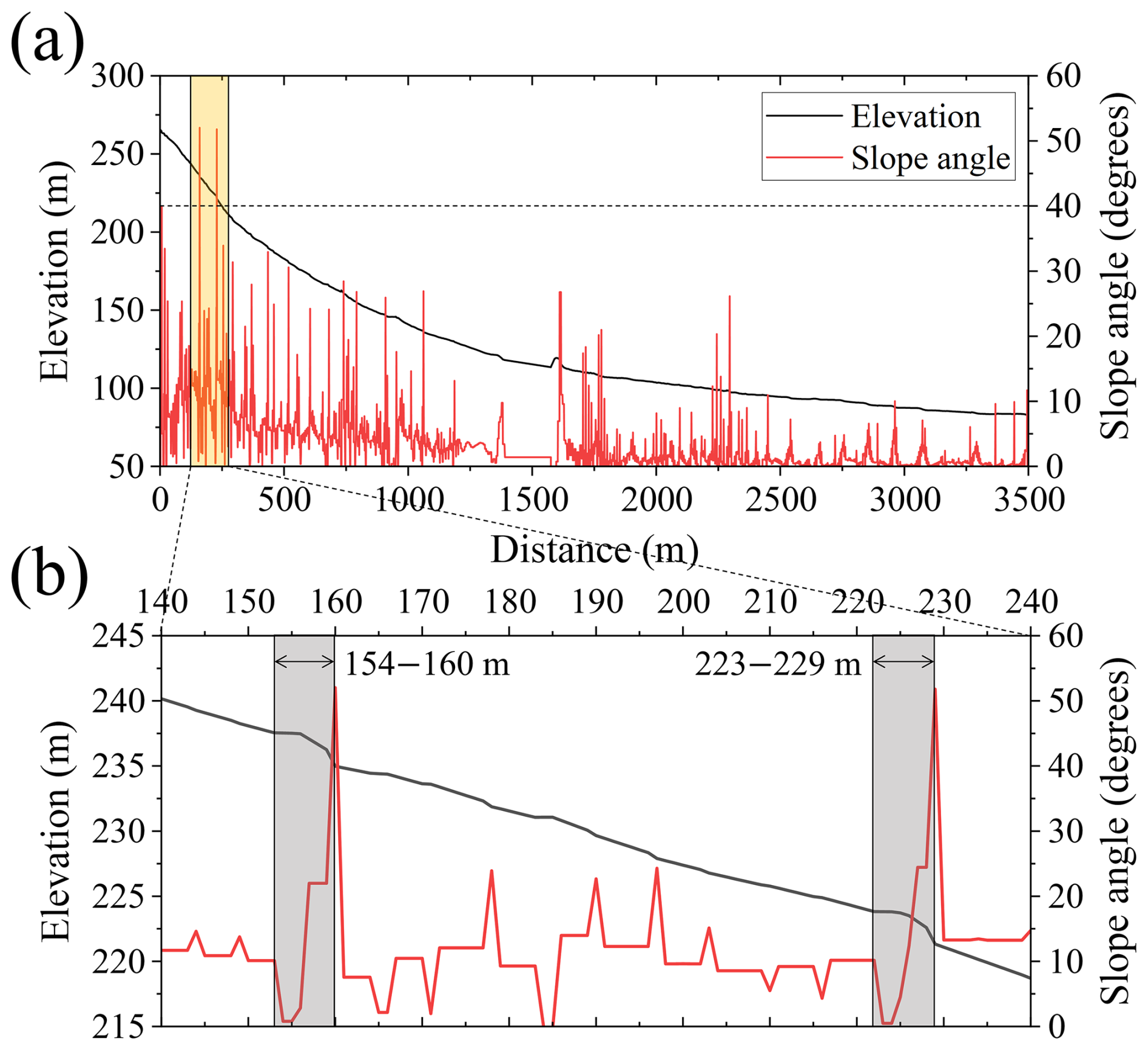
In this study area, although traces of debris flow were clearly observed (Fig. 6), the precise initiation points could not be identified. Therefore, based on Ma et al. (2022), this study assumed that debris flows originated from zones with slopes greater than 40°, as illustrated in Fig. 8.
3.2 Simulation results and discussion
The Sanyang Reservoir basin was simulated based on Sect. 3.1. Figure 9 and movie S1 in the Supplement show debris flow entering the reservoir and causing water level fluctuations. Table 2 summarizes the parameter values used in Fig. 9 and movie S1, which were determined based on the analysis in Sect. 3.1 and previous research on debris flow cases in South Korea (e.g. An et al., 2019; Lee et al., 2022b, 2023). This study assumed that the soil depth was 1 m, and the location of the debris flow initiation was determined based on Fig. 8, assuming that the collapse occurred to the depth of the sediment at that point. However, as the erosion process is typically controlled within the reservoir, this study assumed that erosion induced by debris flow did not occur inside the reservoir. As shown in movie S1, the erosion, entrainment, and deposition processes resulting from the friction between the sediment and the ground during the sediment and debris flow movement on the slope were considered in the numerical simulation as elevation changes. For comparison, movie S2 was produced using the same parameter set as movie S1, with the only difference being that erosion, entrainment, and deposition were neglected. The results shown in movie S2 indicate that the debris flow did not reach the reservoir. This implies that neglecting these processes may lead to an underestimation of the likelihood and potential impact of cascading debris flow–reservoir interactions.
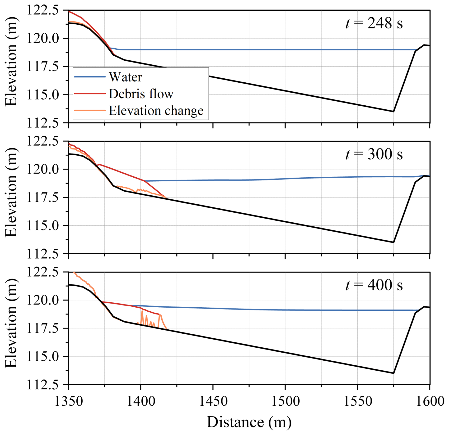
After the collapse of the slope, debris flow entered the reservoir after 245 s. By 300 s, most debris flows had stopped and started depositing within the reservoir (Fig. 9 and movie S1). Only minor, short-lived overtopping occurred in this simulation (approximately 0.5 m3 m−1 at around 290–350 s); nevertheless, the water level in the reservoir rose significantly, threatening the stability of the structure, and continuous waves were observed even after 400 s.
It is essential to consider various conditions and conduct thorough analyses to assess such ungauged basins and predict potential future scenarios. Therefore, this study conducted a two-layer dynamic analysis with different parameter variations based on the range of Voellmy parameters proposed in previous studies (Pirulli and Sorbino, 2008; Hussin et al., 2012; Frank et al., 2015). This study compared and analyzed the wave characteristics observed at points p1, p2, and p3 in Fig. 7 according to the parameter settings. The numerical simulation was conducted with the same water level as the previous case (119 m), and the freeboard to the top of the dam at the flood level was approximately 0.4 m (Fig. 7c).
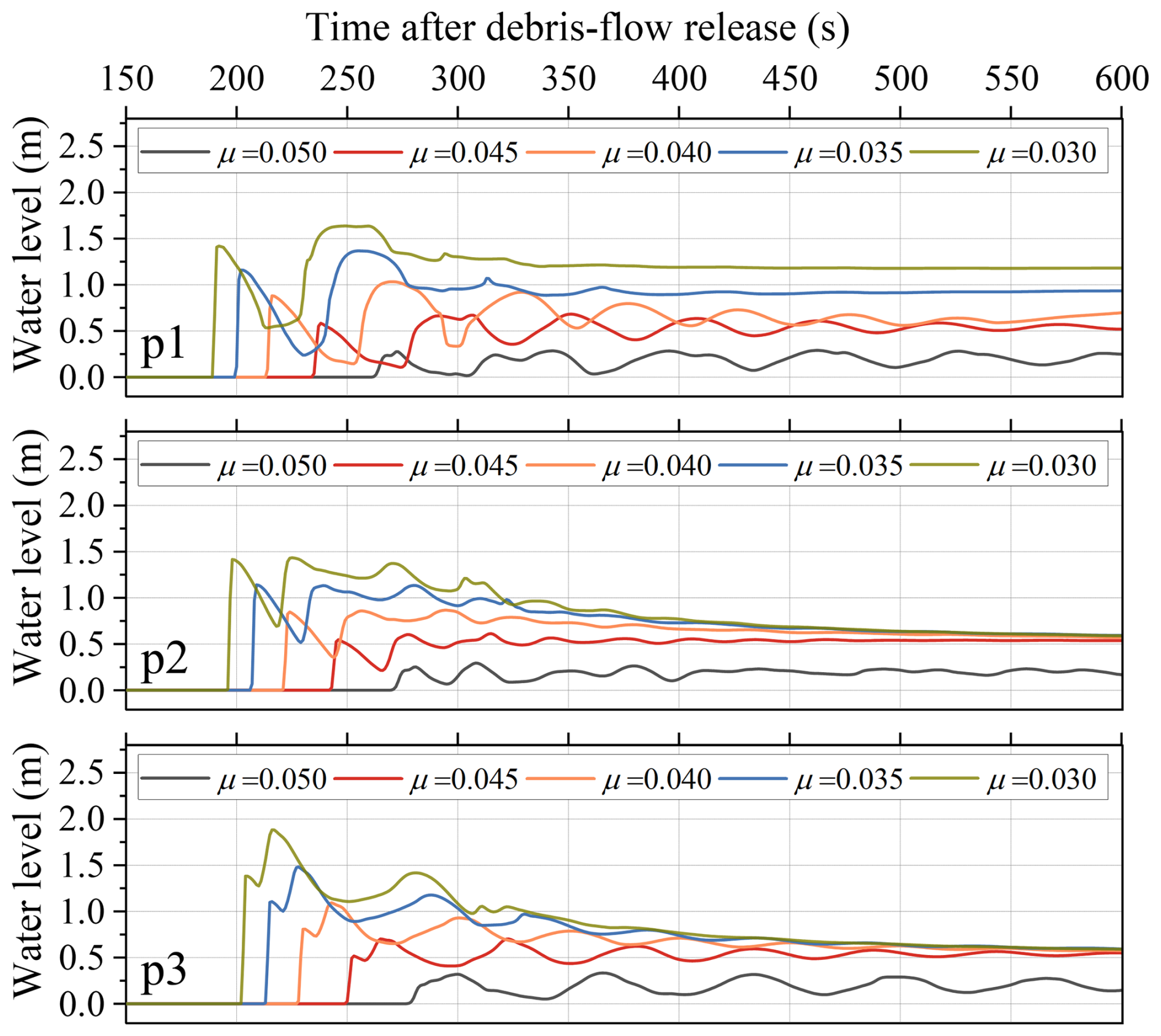
Figure 10Water surface elevation profiles over time at p1, p2, and p3 for different values of the Voellmy parameter μ indicating the differences in wave amplitude and wave speed.
The water level fluctuations over time at p1, p2, and p3 were analyzed by fixing ξ at 500 m s−2 and controlling μ, as shown in Fig. 10. In Voellmy rheology, μ is a parameter representing the viscosity of debris flow, where an increase in μ leads to a slower flow, as previously analyzed by Lee et al. (2020). Previous studies have proposed a range of μ from 0.01 to 0.20; however, this study adjusted it within the range of 0.03 to 0.05, referring to simulation research of debris flow events in South Korea (An et al., 2019; Lee et al., 2022a, b, 2023, 2024). As observed in Fig. 10, even with a μ increment of 0.005, the wave amplitude caused by the inflow of debris flow varied by approximately 0.3 m as the μ value decreased. This variation highlights the sensitivity of wave dynamics to the μ value. As μ increased, the mobility of the debris flow decreased, resulting in a reduction in wave amplitude, illustrating the influence of μ on both debris flow mobility and the resulting wave characteristics. Particularly at p1, for μ = 0.030, the water level rose by up to 1.6 m and remained about 1.2 m higher. This phenomenon occurred because the debris flow was deposited higher than the water level, resulting in an elevation change. Thus, for μ < 0.05, deposition can raise the bed at p1 by up to 1.2 m, reducing the effective storage capacity. These findings suggest that variations in μ can significantly impact water levels. A μ value lower than 0.05 can deteriorate reservoir function due to the debris flow deposition in the reservoir.
For μ < 0.05, the water level at p2 and p3 rose by 0.6–1.9 m and stayed 0.5–0.6 m higher, causing overflow. Consequently, for Sanyang Reservoir, a structure comprising an earthen dam, the presence of highly mobile debris flow with μ lower than 0.05 poses a significant risk of generating waves and potential structure collapse. Among the observed points, p3, closest to the structure, exhibited the highest wave amplitude. This phenomenon is assessed based on the superposition of reflected waves from the structure, and it can cause a significant impact not only on earthen dams but also on concrete dams. However, as observed in Fig. 10, the magnitude of the waves decreased rapidly over time at p1, p2, and p3. The water level of the reservoir stabilized 500 s after the debris flow release.
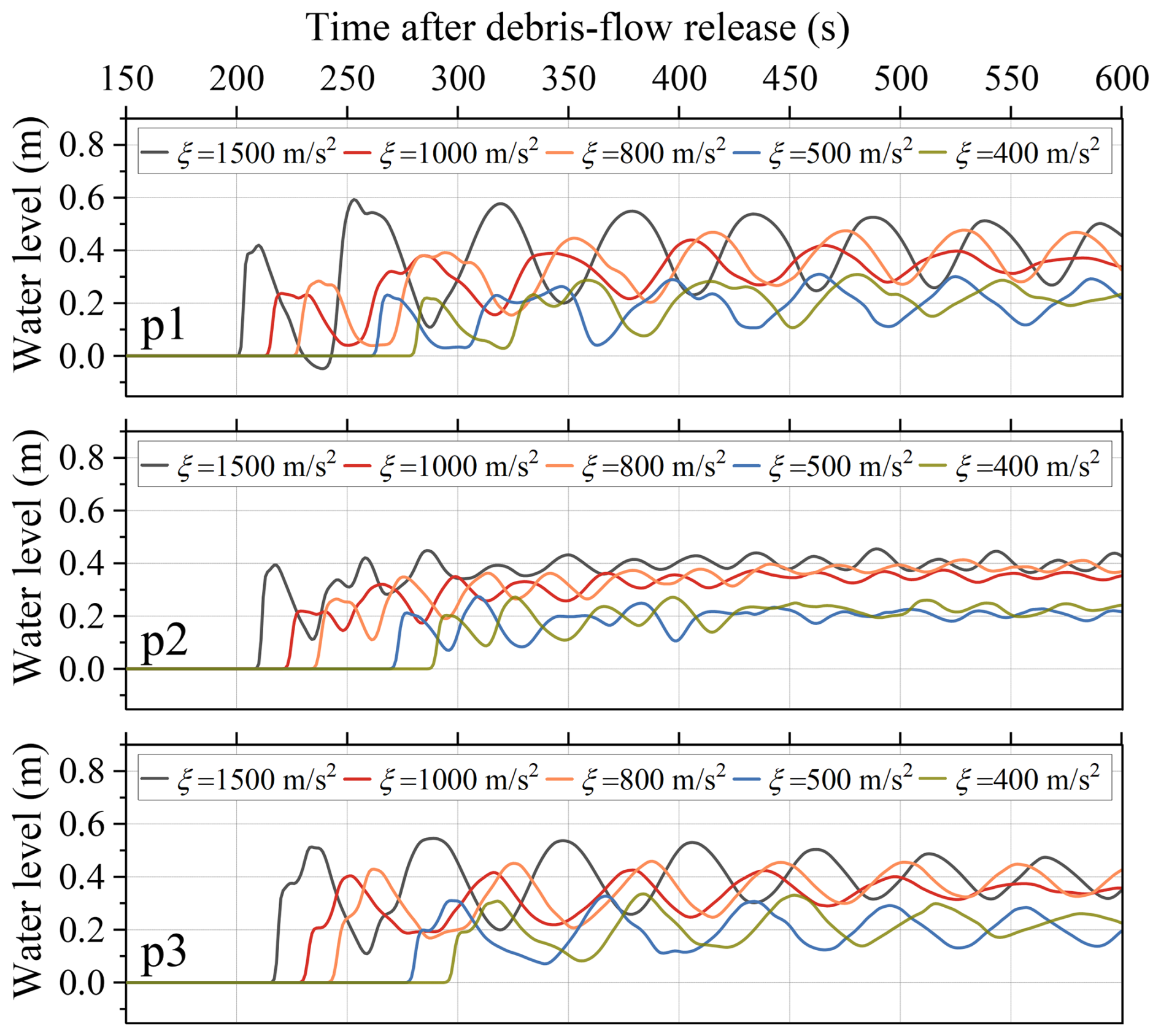
Figure 11Water surface elevation profiles over time at p1, p2, and p3 for different values of the Voellmy parameter ξ indicating the differences in wave amplitude and wave speed.
When μ was fixed at 0.05, and ξ was adjusted, the water level variations over time at p1, p2, and p3 were analyzed as shown in Fig. 11. According to Lee et al. (2020), in Voellmy rheology, ξ is the turbulent friction coefficient, and lower values are associated with a decrease in debris flow velocity. Previous studies proposed a range of ξ from 15 to 2000 m s−2, but this study controlled ξ from 400 to 1500 m s−2, referring to simulation research of debris flow events in South Korea (An et al., 2019; Lee et al., 2022a, b, 2023, 2024). Although ξ decreased, leading to a decline in the mobility of the debris flow, the significant variation in ξ within the applied range, as shown in Fig. 11, did not result in as notable a change in wave height compared to the sensitivity observed with μ. The water level at p1 in Fig. 10 was attributed to topographical changes due to debris flow deposition. However, in Fig. 11, it was analyzed that the continuous wave was transmitted at p1 because the height of the deposited debris flow did not exceed the water level. When ξ was set to 1500 m s−2, the second wave at p1 showed an increase of approximately 0.2 m in wave height compared to the first wave, indicating that the magnitude difference between the first and second waves was amplified depending on the parameter setting. However, regardless of the parameter setting, the second wave at all points (p1, p2, and p3) was more significant in magnitude than the first wave.
According to Fig. 11, even 600 s after the debris flow was released, the water level continues to fluctuate steadily at p1 and p3 due to the waves. However, at p2, the water level stabilized after 400 s because the waves reflected from the structure overlapped with the waves generated by the debris flow entering, and a wave-breaking zone was formed near p2, leading to the water level being the most stable at this point. Thus, Figs. 10 and 11 show distinct simulation results because in Fig. 10, overflow occurred in most cases, causing the energy of the waves to dissipate sufficiently. Therefore, waves with low energy were reflected from the structure, and they had less wave superposition. In Fig. 11, however, overflow was limited, and most wave energy remained in the reservoir. Consequently, at p1 and p3 in Fig. 11, the waves persisted for a long time. These results also indicate that lateral wave spreading and subsequent reflection within the reservoir may substantially affect later wave amplification and long-period water-level oscillations (Heller and Spinneken, 2015; Evers et al., 2019). Although such transverse and reflected wave processes cannot be fully resolved within the present 1D framework, the model remains useful for a first-order estimate of the initial incident wave propagating toward the dam along the principal debris flow path. Therefore, the present wave results should be interpreted as longitudinal screening-level estimates rather than full reservoir-wide predictions.
Table 3Simulation results for each criterion according to changes in the Voellmy rheology.
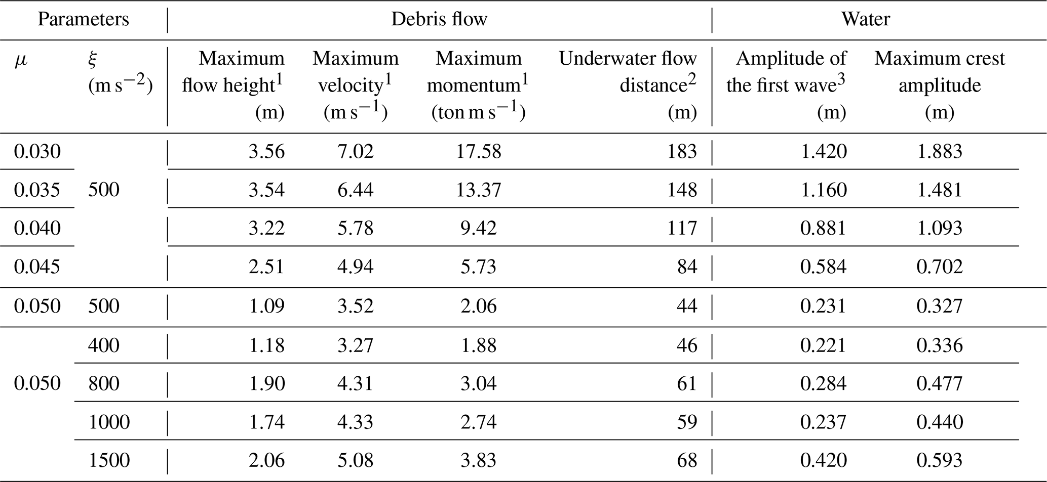
1 Observed near the reservoir (1378 m).
2 Measured from the point where the water meets the ground (1379 m).
3 Observed in p1, Fig. 7 (1450 m).
The analysis of the waves shown in Figs. 10 and 11 and the simulation results of debris flow for each scenario are summarized in Table 3. Additionally, this study has extensively analyzed the situations that may occur due to debris flow into Sanyang Reservoir, not only for the flood level scenario at an elevation of 119 m but also for the high-water level scenario at an elevation of 118 m, as listed in Table S1. As indicated in Tables 3 and S1, as the value of μ decreases, the height and velocity of debris flow increase, leading to an increase in the momentum of the debris flow. In contrast, as ξ increases, the debris flow height, velocity, and momentum generally increase.
Furthermore, after the debris flows into the reservoir, the horizontal flow distance of the debris flow and the amplitude of the first wave caused by the debris flow exhibited an increasing trend with higher debris flow height, velocity, and momentum. Several studies have quantitatively analyzed the dynamic characteristics of debris flow and its interaction with waves (Fritz et al., 2004; Bullard et al., 2019; de Lange et al., 2020). However, they were conducted in laboratory-scale artificial slopes, which limits their direct application to natural slopes. Therefore, this study quantitatively analyzed the relationship between debris flow and waves at the field scale, and the results are presented in Fig. 12 and Table 4.
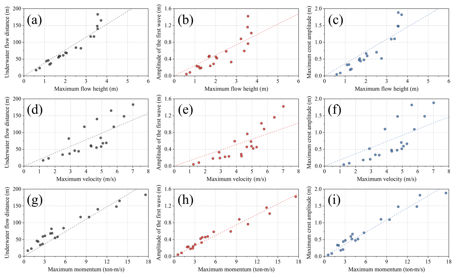
Figure 12Correlation between debris flow characteristics and waves caused by debris flow for the flood-level and high-water level scenarios.
Table 4R2 analysis results between debris flow characteristics and waves caused by debris flow for the flood-level and high-water level scenarios.
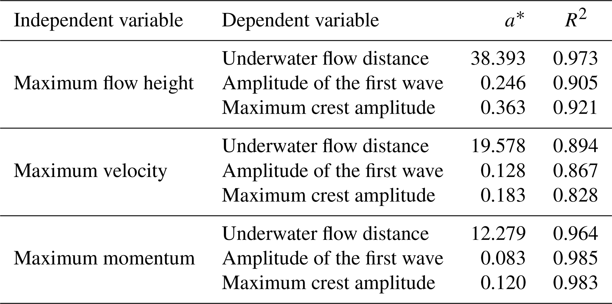
* y = a × x.
Figure 12 and Table 4 are the analysis results based on Table S1 in the Supplement, which comprehensively considers the rainy season (high-water level and flood-level scenarios). Figure 12a, b, and c depict the maximum debris flow height near the reservoir and its relationships with (a) the underwater flow distance of debris flow after inflow into the reservoir, (b) the amplitude of the first wave, and (c) the maximum crest amplitude. Similarly, Fig. 12d, e, and f demonstrate the maximum velocity of debris flow near the reservoir and its relationships with (d) the underwater flow distance, (e) the amplitude of the first wave, and (f) the maximum crest amplitude. Figures 12g, h, and i show the maximum momentum near the reservoir and its relationships with (g) the underwater flow distance, (h) the amplitude of the first wave, and (i) the maximum crest amplitude. As shown in Fig. 12, the maximum flow height correlated well with the underwater flow distance, whereas its correlations with the wave amplitudes and those of the maximum velocity were weaker. The debris flow momentum exhibited high correlations with all three factors. Table 4 summarizes the quantified results of these relationships.
As observed in Fig. 12, the three factors can be derived from the maximum debris flow height by multiplying it by 38.393, 0.246, and 0.363, respectively, with R2 values of 0.973, 0.905, and 0.921, indicating a good ability to predict the underwater flow distance but a relatively lower ability to predict the wave characteristics. The maximum velocity corresponded to R2 values of 0.894, 0.867, and 0.828, which are lower than those of the maximum flow height for all factors. The maximum momentum exhibited R2 values of 0.964, 0.985, and 0.983, comparable to the flow height for the underwater flow distance and the highest for the two wave properties.
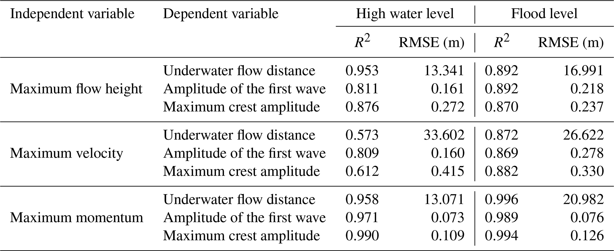
Based on the correlations derived from Table 4, the debris flow data were used to predict the three abovementioned factors. This study analyzed their accuracy for the high-water and flood-level scenarios, as listed in Table 5, where the accuracy of the regression equation derived in Table 4 was quantitatively evaluated using the R2 and the RMSE. R2 was generally higher for the flood-level scenario than for the high-water level scenario. In particular, R2 decreased markedly in the high-water level scenario for the maximum velocity (0.573 and 0.612 for the underwater flow distance and maximum crest amplitude), indicating limited usability. In contrast, the maximum momentum exhibited the most stable accuracy for all metrics, regardless of the water level in the reservoir. Therefore, momentum data are considered adequate for analyzing the characteristics of the waves generated when debris flows into the reservoir, similar to those in Table 4.
Table 5R2 and RMSE analysis results between debris flow characteristics and waves caused by debris flow for two cases: high-water and flood level.
The water level change due to debris inflow according to differences in water-level scenarios is depicted in Fig. 13, and the parameter settings used in this analysis are the same as those listed in Table 2. According to Fig. 13, when debris flows into the reservoir, the water level generally increases by 0.15–0.35 m. However, highly mobile debris flows (μ ≤ 0.035) produced crest amplitudes exceeding the 1.4 m freeboard even at the high-water level (Table S1). In the case of Sanyang Reservoir, which stores water behind an earthen dam, the possibility of dam collapse significantly increases when an overflow occurs. Specifically, reservoirs with small storage, such as Sanyang Reservoir, are expected to experience significant water level fluctuations due to debris flow entering. Therefore, systematic water level control during flood periods is essential in the small reservoirs constructed as earthen dams.
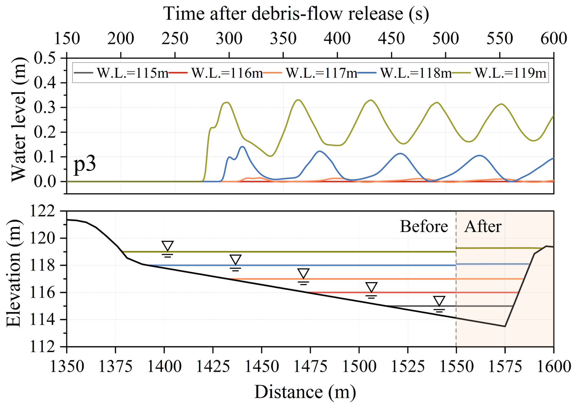
Figure 13Water surface elevation profiles over time at p3 and reservoir level change for different reservoir water levels.
To quantify the dependence of the simulated reservoir impacts on the spatial discretization, grid sensitivity of the Sanyang reference simulation was examined for Δx = 0.125–32 m with a refinement ratio of 2 (Table 6). For Δx ≤ 0.25 m, the debris flow stopped before reaching the reservoir, whereas for Δx = 0.5–16 m the maximum momentum of debris flow increased from 0.55 to 6.9 ton m s−1 and the maximum water-surface rise at p3 from 0.03 to 0.92 m with increasing Δx; at Δx = 32 m, the release zones could not be represented. Longer runout and larger erosion on coarser terrain models have been reported for 2D avalanche simulations (Miller et al., 2022), and first-order schemes are known to over-spread the flow and over-entrain mass (Christen et al., 2008); both effects, together with the threshold-based erosion–deposition closure, likely contribute here. The reservoir impacts reported here are therefore conditional on the adopted 1 m discretization.
Table 6Simulation results for each criterion according to grid spacing (μ = 0.050, ξ = 500 m s−2, water level 119 m).
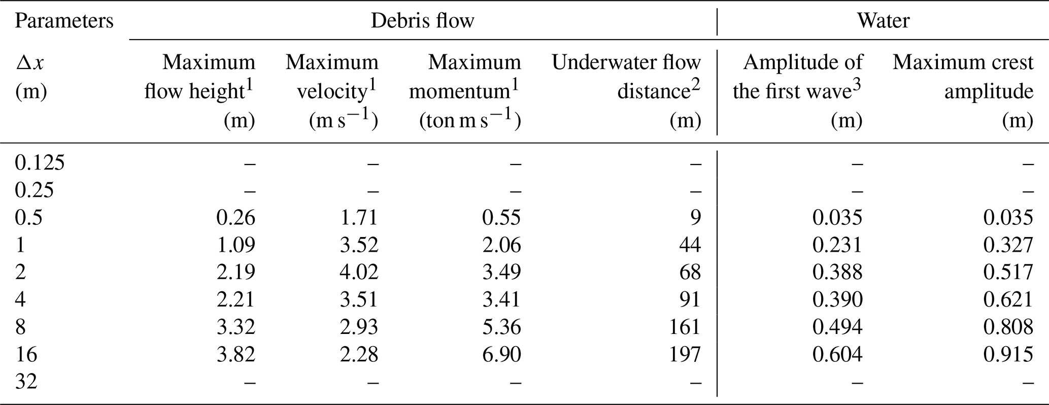
1 Observed near the reservoir (1378 m).
2 Measured from the point where the water meets the ground (1379 m).
3 Observed in p1, Fig. 7 (1450 m).
Computation-only runtimes were measured using 16 OpenMP threads on an AMD Ryzen 9 9950X3D processor (base frequency 4.30 GHz) and reported as medians from three runs, excluding input loading, initialization, and output. The Fig. 2 benchmarks required 52.86 s for Bouchut–Zeitlin (1000 cells, Δx = 0.001 m, 0.5 s simulated), 1696.10 s for Test II (10 000 cells, Δx = 0.01 m, 25 s simulated), and 83.89 s for Test IV (5000 cells, Δx = 0.01 m, 5 s simulated). The Rzadkiewicz et al. (1997) simulation (400 cells, Δx = 0.01 m) required 1.69 s for 0.8 s of simulated time, while the Sanyang reference simulation (2250 cells, Δx = 1 m) required 28.20 s for 600 s of simulated time.
3.3 Limitations and future work
Although results for parameter settings with μ > 0.05 or ξ < 200 m s−2 are not presented in this paper, these cases corresponded to conditions in which the debris flow did not reach the reservoir and therefore did not enter it. Identifying the characteristics of the generated debris flow would be helpful for assessing the occurrence of complex hazards and estimating the magnitude of waves, as suggested by Tables 3 and 4 and Figs. 10 and 11. However, real-time measurement of debris flow properties is practically very difficult, and even when field information is available, direct application remains limited because the Voellmy rheology adopted in this study is a conceptual representation of debris flow behavior. For this reason, scenario-based analysis remains essential, particularly for data-scarce basins such as the present case.
In this context, the present model should be interpreted as a computationally efficient first-order screening tool rather than as a fundamentally new governing formulation or a substitute for high-fidelity 2 or 3D models. The 1D multilayer shallow-water framework was adopted to efficiently represent the dominant longitudinal dynamics of debris flow propagation, momentum evolution, reservoir entry, and the resulting water-level response at field scale. However, this approach cannot resolve transverse topographic effects, lateral spreading of the debris mass, or fully 3D wave generation, amplification, and resonance processes within the reservoir.
Accordingly, further studies should extend the present framework to two- and 3D numerical models in order to analyze complex hazards more precisely, especially in cases where transverse basin geometry, structural failure, overflow, or secondary flooding play an important role. In addition, more rigorous event-based calibration and process-specific validation of erosion, entrainment, and deposition are needed, together with improved methods for evaluating structural stability under wave impact. Accordingly, the present results should be interpreted mainly as first-order estimates of the initial longitudinal wave response toward the dam, whereas transverse spreading, reflection, and later wave amplification within the reservoir require future 2D/3D analysis.
Debris flows entering reservoirs can induce cascading hazards by reducing effective storage capacity, generating impulse waves, and increasing the likelihood of overtopping or structural instability. To assess these processes efficiently at the field scale, this study developed a 1D multilayer shallow-water model that represents debris flow propagation, reservoir entry, debris–water momentum exchange, and wave generation. The model incorporates Voellmy rheology for debris flow motion and an erosion–entrainment–deposition formulation to account for changes in flow volume and momentum during downslope propagation.
The proposed model was evaluated using theoretical benchmark tests and a laboratory-scale experiment involving subaqueous debris flow-induced waves. The validation results, quantified using R2 and RMSE, demonstrated satisfactory model performance in reproducing the overall multilayer flow behavior, water-surface response, and debris flow thickness. Although the depth-averaged formulation cannot fully resolve small-scale oscillations or 3D wave processes, it captured the dominant macroscopic features relevant to debris flow propagation and wave generation. Therefore, the model is appropriate for first-order, field-scale assessment of debris flow-induced reservoir hazards, particularly in data-scarce basins.
Scenario-based simulations of the 2020 Sanyang Reservoir collapse event demonstrated that debris flow-induced waves are highly sensitive to debris flow mobility and reservoir water level. The inclusion of erosion, entrainment, and deposition was particularly important, as neglecting these processes prevented the simulated debris flow from reaching the reservoir. This result indicates that simplified simulations that ignore bed-material entrainment may underestimate both the likelihood of reservoir impact and the resulting wave hazard.
Among the debris flow descriptors examined in this study, maximum momentum provided the most robust indicator of reservoir response. Maximum momentum showed the strongest correlations with the first-wave and maximum crest amplitudes, a correlation with the underwater runout distance comparable to that of maximum flow height, and the most stable accuracy across the two water-level scenarios. This suggests that debris flow momentum can serve as a practical predictor for screening debris flow-induced reservoir wave hazards in data-scarce basins.
The Sanyang Reservoir simulations further indicated that debris inflow can raise reservoir water levels up to 1.9 m, which may be sufficient to induce overflow under flood-level conditions. These findings highlight the vulnerability of small earthen reservoirs with limited freeboard to debris flow-induced cascading hazards, particularly during extreme rainfall events. Therefore, scenario-based assessments that consider debris flow mobility, entrainment, reservoir stage, and available freeboard are essential for supporting reservoir operation and hazard mitigation.
Overall, the proposed model should be interpreted not as a replacement for fully resolved 2D or 3D multiphase models, but as a computationally efficient longitudinal screening framework for field-scale reservoir hazard assessment. Future work should extend the present approach to 2D and 3D analyses, incorporate more detailed bathymetric and event-based field data, and further validate erosion–entrainment–deposition processes and structural responses under wave impact.
Data supporting the research are obtainable from the first author upon reasonable request.
The supplement related to this article is available online at https://doi.org/10.5194/nhess-26-5957-2026-supplement.
SL: Conceptualization, methodology, investigation, software, validation, visualization, writing – original draft preparation. HA: Conceptualization, methodology, software, supervision, writing–reviewing & editing. TK: Methodology, validation. MK: Investigation (field survey), resources (provision of data).
The contact author has declared that none of the authors has any competing interests.
Publisher's note: Copernicus Publications remains neutral with regard to jurisdictional claims made in the text, published maps, institutional affiliations, or any other geographical representation in this paper. The authors bear the ultimate responsibility for providing appropriate place names. Views expressed in the text are those of the authors and do not necessarily reflect the views of the publisher.
This work was supported by the Korea Institute of Geoscience and Mineral Resources (KIGAM) and the Ministry of Agriculture, Food and Rural Affairs (MAFRA). The authors thank the editor and the reviewers for their constructive comments and suggestions, which helped improve the clarity and quality of the manuscript.
During the preparation of this work, the authors used ChatGPT in order to enhance grammatical accuracy and clarity. After using this tool/service, the authors reviewed and edited the content as needed and take full responsibility for the content of the publication.
This work was supported by the Basic Research Project of the KIGAM (grant no. 26-3412) and by the Korea Institute of Planning and Evaluation for Technology in Food, Agriculture and Forestry (IPET) through the Intelligent Agricultural Infra Management for Climate Change Development Program, funded by the MAFRA (grant no. RS-2026-25522713).
This paper was edited by Rachid Omira and reviewed by Matteo Barbini and two anonymous referees.
Abadie, S., Morichon, D., Grilli, S., and Glockner, S.: Numerical simulation of waves generated by landslides using a multiple-fluid Navier–Stokes model, Coast. Eng., 57, 779–794, https://doi.org/10.1016/j.coastaleng.2010.03.003, 2010.
An, H. and Yu, S.: Finite volume integrated surface-subsurface flow modeling on nonorthogonal grids, Water Resour. Res., 50, 2312–2328, https://doi.org/10.1002/2013WR013828, 2014.
An, H., Kim, M., Lee, G., Kim, Y., and Lim, H.: Estimation of the area of sediment deposition by debris flow using a physical-based modeling approach, Quatern. Int., 503, 59–69, https://doi.org/10.1016/j.quaint.2018.09.049, 2019.
Arcement, G. J. and Schneider, V. R.: Guide for selecting Manning's roughness coefficients for natural channels and flood plains, U.S. Government Printing Office, Washington, D.C., U.S. Geological Survey Water-Supply Paper 2339, https://doi.org/10.3133/wsp2339, 1989.
Audusse, E., Bouchut, F., Bristeau, M.-O., Klein, R., and Perthame, B.: A Fast and Stable Well-Balanced Scheme with Hydrostatic Reconstruction for Shallow Water Flows, SIAM J. Sci. Comput., 25, 2050–2065, https://doi.org/10.1137/s1064827503431090, 2004.
Bartelt, P., Buehler, Y., Christen, M., Deubelbeiss, Y., Graf, C., and McArdell, B.: RAMMS–rapid mass movement simulation: A modeling system for debris flows in research and practice, user manual v1.5, debris flow, manuscript update: 31 January 2013, WSL Institute for Snow and Avalanche Research SLF, Davos, Switzerland, 2013.
Benkhaldoun, F., Sari, S., and Seaid, M.: A simple multi-layer finite volume solver for density-driven shallow water flows, Math. Comput. Simulat., 99, 170–189, https://doi.org/10.1016/j.matcom.2013.04.016, 2014.
Bouchut, F. and Zeitlin, V.: A robust well-balanced scheme for multi-layer shallow water equations, Discret. Contin. Dyn. B, 13, 739–758, https://doi.org/10.3934/dcdsb.2010.13.739, 2010.
Boukpeti, N., White, D. J., Randolph, M. F., and Low, H. E.: Strength of fine-grained soils at the solid–fluid transition, Géotechnique, 62, 213–226, https://doi.org/10.1680/geot.9.P.069, 2012.
Bullard, G. K., Mulligan, R. P., Carreira, A., and Take, W. A.: Experimental analysis of tsunamis generated by the impact of landslides with high mobility, Coast. Eng., 152, 103538, https://doi.org/10.1016/j.coastaleng.2019.103538, 2019.
Caleffi, V. and Valiani, A.: Well-Balanced Bottom Discontinuities Treatment for High-Order Shallow Water Equations WENO Scheme, J. Eng. Mech., 135, 684–696, https://doi.org/10.1061/(ASCE)0733-9399(2009)135:7(684), 2009.
Canestrelli, A., Fagherazzi, S., and Lanzoni, S.: A mass-conservative centered finite volume model for solving two-dimensional two-layer shallow water equations for fluid mud propagation over varying topography and dry areas, Adv. Water. Resour., 40, 54–70, https://doi.org/10.1016/j.advwatres.2012.01.009, 2012.
Cesca, M. and D'Agostino, V.: Comparison between FLO-2D and RAMMS in debris-flow modelling: a case study in the Dolomites, WIT Trans. Eng. Sci., 60, 197–206, 2008.
Chen, H.-X., Li, J., Feng, S.-J., Gao, H.-Y., and Zhang, D.-M.: Simulation of interactions between debris flow and check dams on three-dimensional terrain, Eng. Geol., 251, 48–62, https://doi.org/10.1016/j.enggeo.2019.02.001, 2019.
Choi, S.-K., Park, J.-Y., Lee, D.-H., Lee, S.-R., Kim, Y.-T., and Kwon, T.-H.: Assessment of barrier location effect on debris flow based on smoothed particle hydrodynamics (SPH) simulation on 3D terrains, Landslides, 18, 217–234, https://doi.org/10.1007/s10346-020-01477-5, 2021.
Christen, M., Bartelt, P., Kowalski, J., and Stoffel, L.: Calculation of dense snow avalanches in three-dimensional terrain with the numerical simulation program RAMMS, in: Proceedings of the International Snow Science Workshop, Whistler, Canada, 21–27 September 2008, 709–716, https://arc.lib.montana.edu/snow-science/item/119 (last access: 19 November 2026), 2008.
Dai, Z., Li, X., and Lan, B.: Three-dimensional modeling of tsunami waves triggered by submarine landslides based on the smoothed particle hydrodynamics method, J. Mar. Sci. Eng., 11, 2015, https://doi.org/10.3390/jmse11102015, 2023.
de Lange, S. I., Santa, N., Pudasaini, S. P., Kleinhans, M. G., and de Haas, T.: Debris-flow generated tsunamis and their dependence on debris-flow dynamics, Coast. Eng., 157, 103623, https://doi.org/10.1016/j.coastaleng.2019.103623, 2020.
Denlinger, R. P. and Iverson, R. M.: Flow of variably fluidized granular masses across three-dimensional terrain: 2. Numerical predictions and experimental tests, J. Geophys. Res.-Sol. Ea., 106, 553–566, https://doi.org/10.1029/2000JB900330, 2001.
Evers, F. M., Hager, W. H., and Boes, R. M.: Spatial impulse wave generation and propagation, J. Waterw. Port Coast. Ocean Eng., 145, 04019011, https://doi.org/10.1061/(ASCE)WW.1943-5460.0000514, 2019.
Franci, A., Cremonesi, M., Perego, U., Crosta, G., and Oñate, E.: 3D simulation of Vajont disaster. Part 1: Numerical formulation and validation, Eng. Geol., 279, 105854, https://doi.org/10.1016/j.enggeo.2020.105854, 2020.
Franco, A., Moernaut, J., Schneider-Muntau, B., Strasser, M., and Gems, B.: Triggers and consequences of landslide-induced impulse waves – 3D dynamic reconstruction of the Taan Fiord 2015 tsunami event, Eng. Geol., 294, 106384, https://doi.org/10.1016/j.enggeo.2021.106384, 2021.
Frank, F., McArdell, B. W., Huggel, C., and Vieli, A.: The importance of entrainment and bulking on debris flow runout modeling: examples from the Swiss Alps, Nat. Hazards Earth Syst. Sci., 15, 2569–2583, https://doi.org/10.5194/nhess-15-2569-2015, 2015.
Fritz, H. M., Hager, W. H., and Minor, H. E.: Near Field Characteristics of Landslide Generated Impulse Waves, J. Waterw. Port Coast. Ocean Eng., 130, 287–302, https://doi.org/10.1061/(ASCE)0733-950X(2004)130:6(287), 2004.
Gao, Y., Yin, Y., Li, B., Feng, Z., Wang, W., Zhang, N., and Xing, A.: Characteristics and numerical runout modeling of the heavy rainfall-induced catastrophic landslide–debris flow at Sanxicun, Dujiangyan, China, following the Wenchuan Ms 8.0 earthquake, Landslides, 14, 1361–1374, https://doi.org/10.1007/s10346-016-0793-4, 2017.
Guan, X. and Shi, H.: Translational momentum of deformable submarine landslides off a slope, J. Fluid. Mech., 960, A23, https://doi.org/10.1017/jfm.2023.177, 2023.
Han, Z., Chen, G., Li, Y., Tang, C., Xu, L., He, Y., Huang, X., and Wang, W.: Numerical simulation of debris-flow behavior incorporating a dynamic method for estimating the entrainment, Eng. Geol., 190, 52–64, https://doi.org/10.1016/j.enggeo.2015.02.009, 2015.
Han, Z., Su, B., Li, Y., Wang, W., Wang, W., Huang, J., and Chen, G.: Numerical simulation of debris-flow behavior based on the SPH method incorporating the Herschel-Bulkley-Papanastasiou rheology model, Eng. Geol., 255, 26–36, https://doi.org/10.1016/j.enggeo.2019.04.013, 2019.
Han, Z., Su, B., Li, Y., Dou, J., Wang, W., and Zhao, L.: Modeling the progressive entrainment of bed sediment by viscous debris flows using the three-dimensional SC-HBP-SPH method, Water Res., 182, 116031, https://doi.org/10.1016/j.watres.2020.116031, 2020.
Heinrich, P.: Nonlinear Water Waves Generated by Submarine and Aerial Landslides, J. Waterw. Port Coast. Ocean Eng., 118, 249–266, https://doi.org/10.1061/(ASCE)0733-950X(1992)118:3(249), 1992.
Heller, V. and Spinneken, J.: On the effect of the water body geometry on landslide–tsunamis: Physical insight from laboratory tests and 2D to 3D wave parameter transformation, Coast. Eng., 104, 113–134, https://doi.org/10.1016/j.coastaleng.2015.06.006, 2015.
Hungr, O., McDougall, S., and Bovis, M.: Entrainment of material by debris flows, in: Debris-flow Hazards and Related Phenomena, edited by: Jakob, M., and Hungr, O., Springer Berlin Heidelberg, Berlin, Heidelberg, 135–158, https://doi.org/10.1007/3-540-27129-5_7, 2005.
Hürlimann, M., Abancó, C., Moya, J., and Vilajosana, I.: Results and experiences gathered at the Rebaixader debris-flow monitoring site, Central Pyrenees, Spain, Landslides, 11, 939–953, https://doi.org/10.1007/s10346-013-0452-y, 2014.
Hussin, H. Y., Quan Luna, B., van Westen, C. J., Christen, M., Malet, J.-P., and van Asch, Th. W. J.: Parameterization of a numerical 2-D debris flow model with entrainment: a case study of the Faucon catchment, Southern French Alps, Nat. Hazards Earth Syst. Sci., 12, 3075–3090, https://doi.org/10.5194/nhess-12-3075-2012, 2012.
ICOLD: Sedimentation and sustainable use of reservoirs and river systems, Bulletin 147, CRC Press/Balkema, Leiden, the Netherlands, https://doi.org/10.1201/9781003316428, 2023.
Iverson, R. M., Reid, M. E., Logan, M., LaHusen, R. G., Godt, J. W., and Griswold, J. P.: Positive feedback and momentum growth during debris-flow entrainment of wet bed sediment, Nat. Geosci., 4, 116–121, https://doi.org/10.1038/ngeo1040, 2011.
Kim, D.-H., Cho, Y.-S., and Kim, H.-J.: Well-Balanced Scheme between Flux and Source Terms for Computation of Shallow-Water Equations over Irregular Bathymetry, J. Eng. Mech., 134, 277–290, https://doi.org/10.1061/(ASCE)0733-9399(2008)134:4(277), 2008.
Kim, S. W., Chun, K. W., Kim, M., Catani, F., Choi, B., and Seo, J. I.: Effect of antecedent rainfall conditions and their variations on shallow landslide-triggering rainfall thresholds in South Korea, Landslides, 18, 569–582, https://doi.org/10.1007/s10346-020-01505-4, 2021.
Kim, Y., Byun, Y., Kim, Y., and Eo, Y.: Detection of Cochlodinium polykrikoides red tide based on two-stage filtering using MODIS data, Desalin., 249, 1171–1179, https://doi.org/10.1016/j.desal.2009.05.009, 2009.
Krvavica, N.: Re-evaluating efficiency of first-order numerical schemes for two-layer shallow water systems by considering different eigenvalue solutions, Adv. Water. Resour., 137, 103508, https://doi.org/10.1016/j.advwatres.2020.103508, 2020.
Lambe, T. W. and Whitman, R. V.: Soil Mechanics, John Wiley & Sons, New York, ISBN 978-0-471-51192-2, 1991.
Lee, S., An, H., Kim, M., and Lim, H.: Analysis of debris flow simulation parameters with entrainment effect: a case study in the Mt. Umyeon, J. Korea Water Resour. Assoc., 53, 637–646, https://doi.org/10.3741/JKWRA.2020.53.9.637, 2020 (in Korean with English abstract).
Lee, S., An, H., Kim, M., Lee, G., and Shin, H.: Evaluation of different erosion–entrainment models in debris-flow simulation, Landslides, 19, 2075–2090, https://doi.org/10.1007/s10346-022-01901-y, 2022a.
Lee, S., An, H., Kim, M., Lim, H., and Kim, Y.: A simple deposition model for debris flow simulation considering the erosion-entrainment-deposition process, Remote Sens., 14, 1904, https://doi.org/10.3390/rs14081904, 2022b.
Lee, S., An, H., Kim, M., and Kang, T.: Assessment of dam function deterioration due to landslide-debris flows: numerical modeling based on vegetation distribution scenarios, Front. Earth. Sci., 11, 1216096, https://doi.org/10.3389/feart.2023.1216096, 2023.
Lee, S., An, H., Kim, M., and Eu, S.: Preliminary analysis of nocturnal localized heavy rain-induced landslides in Yecheon County, Northern Gyeongsang Province, South Korea, Landslides, 21, 429–435, https://doi.org/10.1007/s10346-023-02182-9, 2024.
Liang, Q. and Marche, F.: Numerical resolution of well-balanced shallow water equations with complex source terms, Adv. Water. Resour., 32, 873–884, https://doi.org/10.1016/j.advwatres.2009.02.010, 2009.
Lim, H.: Erosion-deposition characteristics of debris flow using laboratory experiment and numerical analysis, PhD thesis, Kangwon National University, Republic of Korea, https://www.riss.kr/link?id=T15773029 (last access: 19 November 2026), 2021.
Lyu, L., Xu, M., Wang, Z., Cui, Y., and Blanckaert, K.: A field investigation on debris flows in the incised Tongde sedimentary basin on the northeastern edge of the Tibetan Plateau, Catena, 208, 105727, https://doi.org/10.1016/j.catena.2021.105727, 2022.
Ma, S., Shao, X., and Xu, C.: Characterizing the Distribution Pattern and a Physically Based Susceptibility Assessment of Shallow Landslides Triggered by the 2019 Heavy Rainfall Event in Longchuan County, Guangdong Province, China, Remote Sens., 14, 4257, https://doi.org/10.3390/rs14174257, 2022.
Medina, V., Hürlimann, M., and Bateman, A.: Application of FLATModel, a 2D finite volume code, to debris flows in the northeastern part of the Iberian Peninsula, Landslides, 5, 127–142, https://doi.org/10.1007/s10346-007-0102-3, 2008.
Mergili, M., Jaboyedoff, M., Pullarello, J., and Pudasaini, S. P.: Back calculation of the 2017 Piz Cengalo–Bondo landslide cascade with r.avaflow: what we can do and what we can learn, Nat. Hazards Earth Syst. Sci., 20, 505–520, https://doi.org/10.5194/nhess-20-505-2020, 2020.
Miller, A., Sirguey, P., Morris, S., Bartelt, P., Cullen, N., Redpath, T., Thompson, K., and Bühler, Y.: The impact of terrain model source and resolution on snow avalanche modeling, Nat. Hazards Earth Syst. Sci., 22, 2673–2701, https://doi.org/10.5194/nhess-22-2673-2022, 2022.
Ouyang, C., He, S., Xu, Q., Luo, Y., and Zhang, W.: A MacCormack-TVD finite difference method to simulate the mass flow in mountainous terrain with variable computational domain, Comput. Geosci., 52, 1–10, https://doi.org/10.1016/j.cageo.2012.08.024, 2013.
Pirulli, M. and Sorbino, G.: Assessing potential debris flow runout: a comparison of two simulation models, Nat. Hazards Earth Syst. Sci., 8, 961–971, https://doi.org/10.5194/nhess-8-961-2008, 2008.
Pitman, E. B., Nichita, C. C., Patra, A., Bauer, A., Sheridan, M., and Bursik, M.: Computing granular avalanches and landslides, Phys. Fluids, 15, 3638–3646, https://doi.org/10.1063/1.1614253, 2003.
Pudasaini, S. P.: Dynamics of submarine debris flow and tsunami, Acta. Mech., 225, 2423–2434, https://doi.org/10.1007/s00707-014-1126-0, 2014.
Pudasaini, S. P. and Krautblatter, M.: The mechanics of landslide mobility with erosion, Nat. Commun., 12, 6793, https://doi.org/10.1038/s41467-021-26959-5, 2021.
Rzadkiewicz, S. A., Mariotti, C., and Heinrich, P.: Numerical Simulation of Submarine Landslides and Their Hydraulic Effects, J. Waterw. Port Coast. Ocean Eng., 123, 149–157, https://doi.org/10.1061/(ASCE)0733-950X(1997)123:4(149), 1997.
Schnitter, G. and Weber, E.: Die Katastrophe von Vaiont in Oberitalien, Wasser- und Energiewirtschaft, 56, 61–69, https://doi.org/10.5169/seals-921801, 1964.
Shaffer, J. A. and Parks, D. S.: Seasonal Variations in and Observations of Landslide Impacts on the Algal Composition of a Puget Sound Nearshore Kelp Forest, Bot. Mar., 37, 315–324, https://doi.org/10.1515/botm.1994.37.4.315, 1994.
Shugar, D. H., Jacquemart, M., Shean, D., Bhushan, S., Upadhyay, K., Sattar, A., Schwanghart, W., McBride, S., de Vries, M. V. W., Mergili, M., Emmer, A., Deschamps-Berger, C., McDonnell, M., Bhambri, R., Allen, S., Berthier, E., Carrivick, J. L., Clague, J. J., Dokukin, M., Dunning, S. A., Frey, H., Gascoin, S., Haritashya, U. K., Huggel, C., Kääb, A., Kargel, J. S., Kavanaugh, J. L., Lacroix, P., Petley, D., Rupper, S., Azam, M. F., Cook, S. J., Dimri, A. P., Eriksson, M., Farinotti, D., Fiddes, J., Gnyawali, K. R., Harrison, S., Jha, M., Koppes, M., Kumar, A., Leinss, S., Majeed, U., Mal, S., Muhuri, A., Noetzli, J., Paul, F., Rashid, I., Sain, K., Steiner, J., Ugalde, F., Watson, C. S., and Westoby, M. J.: A massive rock and ice avalanche caused the 2021 disaster at Chamoli, Indian Himalaya, Sci., 373, 300–306, https://doi.org/10.1126/science.abh4455, 2021.
Slingerland, R. L. and Voight, B.: Chapter 9 – Occurrences, Properties, and Predictive Models of Landslide-Generated Water Waves, in: Developments in Geotechnical Engineering, edited by: Voight, B., Elsevier, 317–394, https://doi.org/10.1016/B978-0-444-41508-0.50017-X, 1979.
Stolz, A. and Huggel, C.: Debris flows in the Swiss National Park: the influence of different flow models and varying DEM grid size on modeling results, Landslides, 5, 311–319, https://doi.org/10.1007/s10346-008-0125-4, 2008.
Su, B., Li, Y., Han, Z., Ma, Y., Wang, W., Ruan, B., Guo, W., Xie, W., and Tan, S.: Topography-based and vectorized algorithm for extracting physical quantities in 3D-SPH form and its application in debris-flow entrainment modeling, Eng. Geol., 340, 107693, https://doi.org/10.1016/j.enggeo.2024.107693, 2024.
Su, B., Han, Z., Ma, Y., Li, Y., Ding, H., and Chen, G.: Exploring debris-flow dynamics under basal friction: Insights from an enhanced 3D-SPH coulomb–viscoplastic sliding boundary, Comput. Geotech., 185, 107317, https://doi.org/10.1016/j.compgeo.2025.107317, 2025.
Takahashi, T.: Mechanical Characteristics of Debris Flow, J. Hydraul. Div., 104, 1153–1169, https://doi.org/10.1061/JYCEAJ.0005046, 1978.
Terzaghi, K.: Mechanism of Landslides, in: Application of Geology to Engineering Practice, Berkey Volume edn., edited by: Paige, S., Geological Society of America, New York, 83–123, https://doi.org/10.1130/Berkey.1950.83, 1950.
VanDine, D. F. and Bovis, M.: History and Goals of Canadian Debris Flow Research, A Review, Nat. Hazards, 26, 67–80, https://doi.org/10.1023/A:1015220811211, 2002.
Voellmy, A.: Über die Zerstörungskraft von Lawinen, Bauztg., 73, 159–165, 1955.
Wang, F.-W., Zhang, Y.-M., Huo, Z.-T., Matsumoto, T., and Huang, B.-L.: The July 14, 2003 Qianjiangping landslide, Three Gorges Reservoir, China, Landslides, 1, 157–162, https://doi.org/10.1007/s10346-004-0020-6, 2004.
Wieczorek, G. F. and Glade, T.: Climatic factors influencing occurrence of debris flows, in: Debris-flow Hazards and Related Phenomena, edited by: Jakob, M., and Hungr, O., Springer Berlin Heidelberg, Berlin, Heidelberg, 325–362, https://doi.org/10.1007/3-540-27129-5_14, 2005.
Zhao, Y., Meng, X., Qi, T., Li, Y., Chen, G., Yue, D., and Qing, F.: AI-based rainfall prediction model for debris flows, Eng. Geol., 296, 106456, https://doi.org/10.1016/j.enggeo.2021.106456, 2022.
Zhou, G. G. D., Li, S., Song, D., Choi, C. E., and Chen, X.: Depositional mechanisms and morphology of debris flow: physical modelling, Landslides, 16, 315–332, https://doi.org/10.1007/s10346-018-1095-9, 2019.