Large discrepancies between event- and response-based compound flood hazard estimates

Most flood hazard assessments follow the event-based approach, assuming that the probability of flooding approximates the probability of flood drivers. However, this approach neglects information about the temporal and spatial variability of flood drivers and flood processes such as water propagation inland and its interaction with topography. The response-based approach accounts for these factors by using a large number of flood events that allow the calculation of flood probabilities. Here, we compare differences in flood hazards between the event- and response-based approaches for a case study in Gloucester City (NJ, U.S.). We find that compound events with return periods less than 20 years can produce the 100-year (i.e., 1 % annual exceedance probability) flood depths in large areas of the city. This is caused by the temporal and spatial characteristics of these events, such as prolonged high coastal water levels and rainfall fields with higher rainfall rates over urbanized areas. These event characteristics are not included in extreme value models of the flood drivers and are commonly simplified by using a single design event. However, flood hazards largely depend on them, introducing large discrepancies in resulting flood hazards if neglected. The temporal and spatial variabilities of flood drivers need to be incorporated in flood hazard assessments to produce robust estimates.

1 Introduction

Coastal communities worldwide are facing increasing flood hazards from rising sea levels (Taherkhani et al., 2020; Wing et al., 2024) and extreme events such as tropical cyclones (Nederhoff et al., 2024). The rapid development in coastal zones compared to inland areas is also contributing to increasing the exposure to flooding of people and assets (Cosby et al., 2024), making flooding the costliest hazard for coastal zones. In the U.S. alone, damages from tropical cyclones exceeded USD 1.5 trillion in total since 1980. and account for more than 50 % of total disaster costs every year (NCEI, 2024). Therefore, developing adaptation and mitigation strategies to reduce flood impacts and increase the resilience of coastal communities is essential.

The most common framework for estimating coastal flood risks is the one defined by the Intergovernmental Panel on Climate Change (IPCC) in the Special Report on Managing the Risks of Extreme Events and Disasters to Advance Climate Change Adaptation (SREX), in which risks are defined as a function of the hazard, exposure, and vulnerability (IPCC, 2012). In the context of coastal flooding, quantifying the likelihood of coastal flood hazards is thus the first step to estimating flood risks and impacts. However, there is no standard approach to quantifying flood hazards, resulting in a variety of methods being used, and discrepancies between them are not well understood. There are two main general approaches to estimating flood hazards, namely event-based and response-based. However, there is also no clear consensus in the literature regarding the terminology used to distinguish these two approaches. The event-based method is often referred to as the “design-storm” or “deterministic” approach. In contrast, the response-based approach has been described using terms such as “probabilistic”, “stochastic”, “continuous”, or “weather-generator-based”. Some of these terms (particularly “probabilistic”) are also used in other contexts, such as to describe flood maps that incorporate uncertainty in model parameters, which can lead to ambiguity in their interpretation (Alfonso et al., 2016; Di Baldassarre et al., 2010; Bates et al., 2004). Therefore, in this study, we adopt the term “response-based”, consistent with its usage in the structural reliability literature (Gouldby et al., 2014; Jane et al., 2022).

The event-based approach is the most commonly used. It consists of estimating first the probability of the flood driver(s), selecting one event of desired probability (e.g., 1 % annual exceedance probability (AEP)), and assuming that the flooding resulting from that event approximates the occurrence probability of the event (i.e. one-to-one relationship). This approach can be applied for the full range of probabilities of events, from low to high, and produce what is also known as probabilistic flood hazard estimates (e.g., Kupfer et al., 2024). However, the most commonly used benchmark event for flood hazards is the 1 % AEP, often referred as the 100 year return period or in other words, an event that has a 1 in 100 chance of being equaled or exceeded in any given year. In the U.S., the event-based approach has been widely used by the Federal Emergency Management Agency (FEMA) to produce the 1 % AEP flood elevations for both coastal and inland flood mapping, which serve as the basis for regulatory floodplain for management and planning (FEMA, 2022). For inland flooding, FEMA applies the event-based approach that starts by defining a design rainfall storm, typically derived from NOAA Atlas 14 which provides rainfall depths for specific probabilities (e.g., 1 % AEP, 24-h storms). The design storms are used in hydrologic models to simulate runoff, with the resulting hydrographs then routed through hydraulic models to estimate flood depths and extents. In some cases, inland flooding is instead mapped using the 1 % AEP river discharge estimated from stream gauges. Similarly for coastal regions, a design event is selected from the distribution of coastal water levels to estimate the 1 % AEP regulatory floodplain. In regions affected by tropical cyclones (TCs), FEMA further implements the Joint Probability Method (JPM) to construct a synthetic storm climatology. This involves statistically sampling combinations of key storm parameters (e.g. central pressure deficit, radius to maximum winds, forward speed) based on their joint probability distributions. These synthetic events are then dynamically downscaled to the coast and exceedance probabilities of coastal water levels are calculated based on the probabilities of the storm characteristics. Although the JPM approach might reduce the uncertainties related to estimating the likelihood of low-probability coastal water level events by increasing the sample size of these events, in both cases, the probability of the event is assumed to approximate the probability of flooding (FEMA, 2022). Selecting a single event that approximates the 1 % AEP floodplain might not be a simple task. On one hand, observational records of flood drivers are typically shorter than 100 years, making it necessary to apply statistical extreme value models to estimate the likelihood of events and to extrapolate beyond the observed data to characterize low-probability events (such as the 1 % AEP) that may not be captured in the historical record. Statistical extreme value models focus only on the magnitude of the drivers, and the temporal and spatial variability during events are neglected (e.g., Jane et al., 2020; Moftakhari et al., 2019). In the case of coastal water levels, the lack of information about the temporal evolution of the event has been commonly simplified using different approaches such as selecting one historical event as a “design event” and rescaling its time series to the desired magnitude, e.g., matching the 1 % AEP event (Dawson et al., 2005; Peña et al., 2023; Wadey et al., 2015); assuming a triangular or sine shape (e.g., Vousdoukas et al., 2016; Moftakhari et al., 2019); or defining a mean hydrograph shape from hindcast data (Dullaart et al., 2023). However, neglecting the temporal variability of coastal water levels can introduce large uncertainties in estimated flooding (Kupfer et al., 2024; Quinn et al., 2014; Santamaria-Aguilar et al., 2017). Similarly, for rainfall and river discharge, traditional approaches defined a single “design storm” or “design event” to represent the temporal and spatial patterns of these drivers (i.e. a representative event structure). However, some recent studies have shown that relying on a single “design storm”, overlooking the variability in event structure across multiple storms, can underestimate flood hazards and associated impacts (Baer, 2025; Perez et al., 2024). Furthermore, when flooding results from multiple drivers (e.g., tropical cyclones producing both storm surge and heavy rainfall), various combinations of driver magnitudes may share the same probability yet lead to differing flood depths and extents (see e.g. Peña et al., 2023). On the other hand, flooding (i.e., the response) also depends on other factors beyond the flood driver characteristics, such as topography and associated water dynamics.

In contrast, the response-based approach can account for all these factors to produce more robust flood hazard estimates (Baer, 2025; Perez et al., 2024). This approach involves simulating flooding from many events, enabling the calculation of empirical flood depth distributions at different points in the floodplain. However, the response-based approach also has limitations. First, a large set of events is needed, which is unavailable in observed records that rarely span more than a few decades (Ponte et al., 2019). Therefore, synthetic event datasets generated through dynamical modelling and/or complex statistical frameworks are necessary (Gori et al., 2020; Kim et al., 2023; Maduwantha et al., 2025). Second, this approach is computationally more demanding and hence it has been rarely used in the past, but it is becoming more feasible due to advances in computing power (Gori et al., 2020) and new computationally efficient flood models (Bates et al., 2005; Leijnse et al., 2021). Although the response-based approach provides more robust estimates of flood depths at the household level (or at single points), the corresponding flood extent does not represent the floodplain of a single event, which might be needed for some applications such as emergency management, government budgeting for natural disasters, and insurance market. Coastal flooding often occurs from a combination of different drivers such as storm surges, wave runup, tides, heavy precipitation, and river discharge; so-called compound events. In fact, the risk of compound flooding from storm surges and rainfall is larger in the Atlantic and Gulf coasts of the U.S. (Wahl et al., 2015). However, FEMA has not planned to incorporate compound flood modelling in coastal regions or transition to a full response-based approach to estimate coastal compound flood hazards. For inland regions, FEMA is working to develop a methodology to transition to response-based (probabilistic) estimates (Lehman, 2023). Although FEMA provides some guidelines to map the 1 % AEP floodplain, Mapping Partners can deviate from the guidelines if they consider it appropriate (FEMA, 2022). Thus, choosing between an event-based or response-based approach to estimate flood hazard is a decision that can be made. However, this choice is challenging to make in advance since it is unclear how closely the 1 % AEP event (in terms of the flood drivers) approximates the 1 % AEP flood (in terms of the response). To our knowledge, the differences in flood hazard estimates between these two approaches have only been evaluated for rainfall flooding (Baer, 2025; Perez et al., 2024; Winter et al., 2020), but remain unexplored for compound coastal flooding. For the latter, selecting a single 1 % AEP design event is particularly challenging, as multiple combinations of flood drivers can yield the same joint exceedance probability. This challenge has sometimes been addressed through the introduction of ambiguous constructs, such as the “most likely” event, which attempts to identify a representative scenario among equally probable combinations based on the density of observed events (Jane et al., 2022; Moftakhari et al., 2019; Salvadori et al., 2011).

Here, we explore the degree of linearity in the relationship between events of 1 % chance of occurring any year and flooding of equal probability, from compound events of precipitation and estuarine water levels in a case study for Gloucester City, New Jersey. We first assess the variability in flooding from different synthetic 1 % AEP events of equal probability but different magnitudes, and temporal and spatial evolutions, to quantify the uncertainties related to using a single design event for estimating flood hazards. Then, we compare flood extents and depths from the 1 % AEP events with the response 1 % AEP flood. Finally, we investigate which individual compound events can cause the response 1 % AEP flood depth in different parts of the study area.

2 Study site

Our study site is Gloucester City, New Jersey, a small municipality located in the Delaware estuary (Fig. 1) frequently affected by pluvial and coastal flooding (Smith, 2023). We selected this study site based on the exploratory scoping analysis of Helgeson et al. (2025) for place-based convergence research. Gloucester City is bordered by water on multiple sides, with the Delaware River to the west and Newton Creek and Little Timber Creek to the north and south, respectively. The catchments of these two creeks are relatively small (147.45 km²), extending slightly beyond the city's administrative boundaries and draining into the Delaware River to the north and south of Gloucester City. Alongside the confluence of Newton Creek, Little Timber Creek, and the Delaware River, the city's low-lying terrain, with elevation <10 m above NAVD88, makes it especially susceptible to compound flooding from rainfall and elevated estuarine water levels, including storm surges, tides, and river discharge. In addition, these catchments are highly urbanized (see Fig. S2 in the Supplement) and the sewer and stormwater systems are combined. The municipalities in these catchments have faced long-standing issues with repetitive flooding of streets and properties caused by inadequate stormwater drainage systems and tidal influences in the outflow discharging systems (Smith, 2023).

The FEMA Risk Map and Report, dated in 1979 and updated in 2016, defines a coastal and riverine 1 % AEP floodplain (i.e., Special Flood Hazard Area, SFHA) that covers large areas of the city, including five essential facilities (FEMA, 2016). Between 1974 and 2016, Gloucester City was subject to five federally declared flood-related disasters. Despite this, only 94 properties were enrolled in the National Flood Insurance Program (NFIP) as of 2016, according to data from OpenFEMA. Of these, 76 properties were located within the SFHA. Based on the National Structure Inventory, Gloucester City contains a total of 3341 single-family homes, 148 of which are situated within the SFHA. Gloucester City has been facing problems with repetitive localized pluvial and coastal flooding for years (Fig. S5), further exacerbated by an inadequate stormwater drainage system (Smith, 2023). This is also highlighted in the FEMA Risk Map, in which an intersection of the city outside the SFHA is marked together with a photo of flooding from an event in 2009 (FEMA, 2016; Fig. S21).

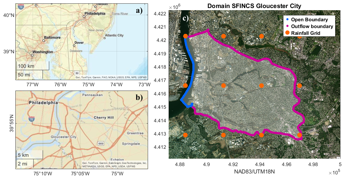
Figure 1 Location of Gloucester City (NJ, U.S.) within the inner part of the Delaware estuary (a–b). The map (c) shows the flood model domain covering the catchments of Newton Creek and Little Timber Creek that surround the study site of Gloucester City. The blue line shows the location of the open boundary of the flood model along the Delaware River, the purple line is the inland outflow boundary, and the orange dots are the grid nodes of the rainfall forcing [NAD83/UTM18N. Sources (a): Esri, TomTom, Garmin, FAO, NOAA, USGS, EPA, NPS, USFWS | Powered by Esri. Sources (b): Esri, TomTom, Garmin, SafeGraph, GeoTechnologies, Inc, METI/NASA, USGS, EPA, NPS, USDA, USFWS | Powered by Esri. Source (c): Esri | Powered by Esri].

3 Data and Methods

We investigate differences in flooding between the event- and response-based approaches by simulating flooding from a large number (5000) of compound events that allow estimating the empirical distribution of flooding and comprise several events that have a 1 % chance of happening in any year. We created a catalog of 5000 synthetic compound events (more details on those events are provided in Sect. 3.1) following the framework of Maduwantha et al. (2025), which provides storm tide hydrographs and rainfall fields.

The joint probabilities of these events were calculated using the multivariate statistical framework of Maduwantha et al. (2024). We use the reduced-complexity flood model SFINCS (Super-Fast INundation of CoastS) to simulate pluvial and coastal flooding from the synthetic events in the study area (Fig. 1). Details of the flood model configuration and input data are described in Sect. 3.2, and the model validation is presented in Sect. 3.3.

3.1 Synthetic compound events

We need a large sample of compound events to estimate the response-based flood hazard, in which the probability of certain flood thresholds being exceeded is calculated for each model cell based on the empirical distribution. We use both the multivariate statistical framework of Maduwantha et al. (2024) and the event generation approach of Maduwantha et al. (2025) to derive a catalog of synthetic compound events, including information on rainfall fields and coastal water levels along the Delaware River at Gloucester City. Maduwantha et al. (2024) developed a new multivariate statistical framework to estimate joint probabilities of rainfall and non-tidal residuals (NTR) using copulas, accounting for the dependencies between these two flood drivers but also stratifying the extreme events by the different storm types that generate them, namely tropical cyclones and non-tropical cyclones (Fig. 2), since these show different statistical characteristics. Non-tropical events dominate the low return levels, while tropical cyclones have a stronger effect on large return levels, such as the ones associated with events of 1 % chance occurring in any given year. Accounting for the different statistical characteristics of events caused by these different storm types, the joint probability analysis avoids mischaracterization of both low and high-return level events.

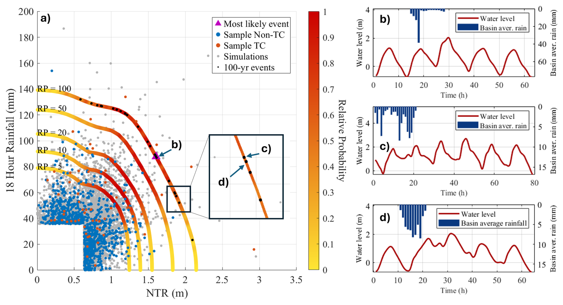
Figure 2 (a) Joint probabilities of non-tidal residual (NTR) and 18 h rainfall accumulation. Blue dots show the historical non-tropical cyclone events, red dots show the historical tropical cyclone events, and grey dots the 5000 synthetic events generated for this study. All synthetic events (grey points) have assigned water level hydrographs and rainfall fields to be used as boundary conditions for SFINCS. (b), (c) and (d) show as an example the time series of three 1 % AEP (100-year) events (black dots along the 100-year isoline); (b) shows the time series of the “most likely” event, marked as a purple triangle in (a); (c) shows the 1 % AEP (100-year) event that produces the largest flood from all 1 % AEP (100-year) events (black dots in (a); and (d) shows the 1 % AEP (100-year) event that produces the smallest flood from all 1 % AEP (100-year) events. Water levels are referenced to NAVD88.

For the catchments of our study site, Maduwantha et al. (2024) used around 120 years of in-situ rainfall and coastal water level measurements to estimate the joint probabilities of the flood drivers, namely rainfall and NTR. Since our study site is located in the mid-estuarine region of the Delaware Estuary, the NTR reflects contributions from both fluvial discharge and coastal storm surge, as well as their nonlinear interactions. We opted not to disaggregate the NTR into riverine and coastal components due to the substantial complexity of their coupled dynamics and the additional challenges this would introduce into the structure and parameterization of the multivariate statistical model. Maduwantha et al. (2024) found the largest dependency between NTR peak and rainfall exists for 18-h rainfall accumulation. Since single-point rainfall might not be representative of the entire catchment, they also used 40 years of 4 km gridded rainfall data from the Analysis of Period of Record for Calibration (AORC, Kitzmiller et al., 2018) of the corresponding catchments to obtain spatial rainfall information and average catchment values. Observed compound events were identified using the Peaks Over Threshold (POT) approach combined with a two-sided conditional sampling method. Thresholds were set to capture an average of five events per year, providing a balance between sufficient sample size and an appropriate representation of the tail distribution. These thresholds also maximized the statistical dependence between variables. Additionally, the conditional sampling method includes events where one variable is not extreme, allowing for coverage of the full range of driver magnitudes, including those that may not lead to flooding. Further details about the multivariate statistical framework can be found in Maduwantha et al. (2024).

Maduwantha et al. (2025) developed an approach to generate synthetic compound events based on the joint probability distribution from the previous analysis and by considering the temporal and spatial information of historical events. From the joint probability distribution, they derived a sample of 5000 events, ensuring that the proportion of observed tropical and non-tropical events is retained in the synthetic data (Fig. 2). Dynamic flood models such as SFINCS also require information about the temporal evolution of events, namely time series of both coastal water levels and rainfall fields. For that, Maduwantha et al. (2025) used the time series of historical events to generate new time series for the synthetic event set. For each synthetic event, the time series of a historical event is selected randomly accounting for their proximity in the joint probability space, and thus accounting for differences in the temporal and spatial characteristics of these events depending on their magnitude. The historical event is then rescaled to the desired magnitude of the synthetic event. The rescaled NTR time series is then combined with a mean sea-level value and a tidal curve while accounting for seasonality. The NTR hydrograph (i.e., time series) and the selected tidal curve are combined by selecting the lag from the observed events in order to account for the tide-surge interaction. Likewise, the synthetic rainfall field is combined with the synthetic water level hydrograph selecting a time lag between peaks based on the observed historical events. The synthetic compound events were validated by comparing observed and simulated distributions of key event characteristics (e.g. magnitude of the peaks, duration, times lags, intensities) and dependencies among them, finding a good agreement between observed and simulated events. Further details about the methodology used to generate the synthetic compound events can be found in Maduwantha et al. (2025) and the codes in Maduwantha (2026).

Of the 5000 synthetic compound events used, 25 lie along the 100-year (1 % AEP) isoline (i.e. with a 1 % probability of happening any given year; Fig. 2) To further investigate differences in flood hazard estimations between approaches, we also define a “design event” from all the 100-year events following the “most likely” approach for multivariate events (Jane et al., 2022; Moftakhari et al., 2019). This approach selects one event in the isoline based on the density of observed events along it (Salvadori et al., 2011), identifying this event as the most representative scenario (“most likely”) among the equally probable combinations along the isoline. The water levels at the Delaware River boundary of the model are also affected by the tidal variability, which is periodic and thus its probability is not included in the multivariate extreme method of Maduwantha et al. (2024) for stochastic variables. We estimate the likelihood of tidal levels based on the predicted tides of the 19-year period from 2003 to 2021 to include long-term tidal variations such as the perigean and nodal cycles (4.4 and 18.6 years). Predicted tidal levels are generated based on the annual harmonic analysis performed by Maduwantha et al. (2024) including nodal corrections estimated from astronomical parameters (see Codiga, 2011 for further information about the tidal harmonic analysis using UTide). We focus only on the likelihood of high tide peaks since flooding is more likely at these levels, but it is important to notice that the synthetic events are generated by combining the NTR peak and the high tide peak accounting for the historical distribution of time lags, and thus accounting for tide-surge interactions (Maduwantha et al., 2025).

The tidal regime in our study region is mixed semidiurnal, with two high tides per day, but one is higher than the other. We calculate the Mean Higher High Water (MHHW) level following the definition by the National Oceanic and Atmospheric Administration (NOAA) to provide an average level of the largest tidal level that happens once a day. MHHW is estimated as the average of the higher high water peaks of each day over a specified period, which in our case is the 19-year period from 2003 to 2021 (instead of the National Tidal Datum Epoch (1983–2001) used by NOAA), in order to provide an updated estimate of MHHW and better representing present-day tidal conditions (Fig. 3). Although the largest variability of tidal levels is at daily scale, tidal high waters also vary at fortnightly, seasonal, and interannual time scales. Therefore, we also estimate the mean spring tidal levels as the average of the largest high-water levels every 14 d and the average “king tide” as the mean of the annual largest tide over the 19-year period (Fig. 3).

Previous studies pointed to periods of increases in both high-tide flooding (Thompson et al., 2021) and extreme coastal flooding (Enriquez et al., 2022) caused by the nodal and perigean modulations of high-tide levels. Although these modulations are at longer time scales (4.4 and 18.6 years), the next peaks of both cycles will occur between 2025 and 2034 for diurnal and semidiurnal regimes. Since the tidal regime in our study site is mixed semidiurnal, the peaks of these two long-term tidal cycles are expected to occur within that period. To evaluate potential impacts of the long-term tidal modulations on the compound flood analyses, we estimate the 4.4- and 18.6-year tidal cycles following the approach of Enriquez et al. (2022) for the tide-gauge records of Philadelphia. We fit a least-squares regression to the annual king tidal levels (Eq. 1) of the last 60 years of record as suggested by Haigh et al. (2011).

$$\begin{array}{}\text{(1)}& \begin{array}{rl}H\left(t\right)& =\mathit{\beta }+{\mathit{\beta }}_{\mathrm{1}}\left(t\right)+{\mathit{\beta }}_{\mathrm{2}}\cos \left({\displaystyle \frac{\mathrm{2}\mathit{\pi }}{\mathrm{4.4}}}t\right)+{\mathit{\beta }}_{\mathrm{3}}\sin \left({\displaystyle \frac{\mathrm{2}\mathit{\pi }}{\mathrm{4.4}}}t\right)\\ & +{\mathit{\beta }}_{\mathrm{4}}\cos \left({\displaystyle \frac{\mathrm{2}\mathit{\pi }}{\mathrm{18.6}}}t\right)+{\mathit{\beta }}_{\mathrm{5}}\sin \left({\displaystyle \frac{\mathrm{2}\mathit{\pi }}{\mathrm{18.6}}}t\right)\end{array}\end{array}$$

Where H(t) are the king tides of each year t, β₀ is a constant term, β₁ is the linear term, β₂ and β₃ are the amplitudes of the perigean cycle and β₄ and β₅ are the amplitudes of the nodal cycle. Based on the fitted regression, we estimate the amplitudes of both the perigean and nodal cycles, and the timing of the next peak of both cycles for our study region; this provides a better estimation of the present-day probability of large astronomical tides.

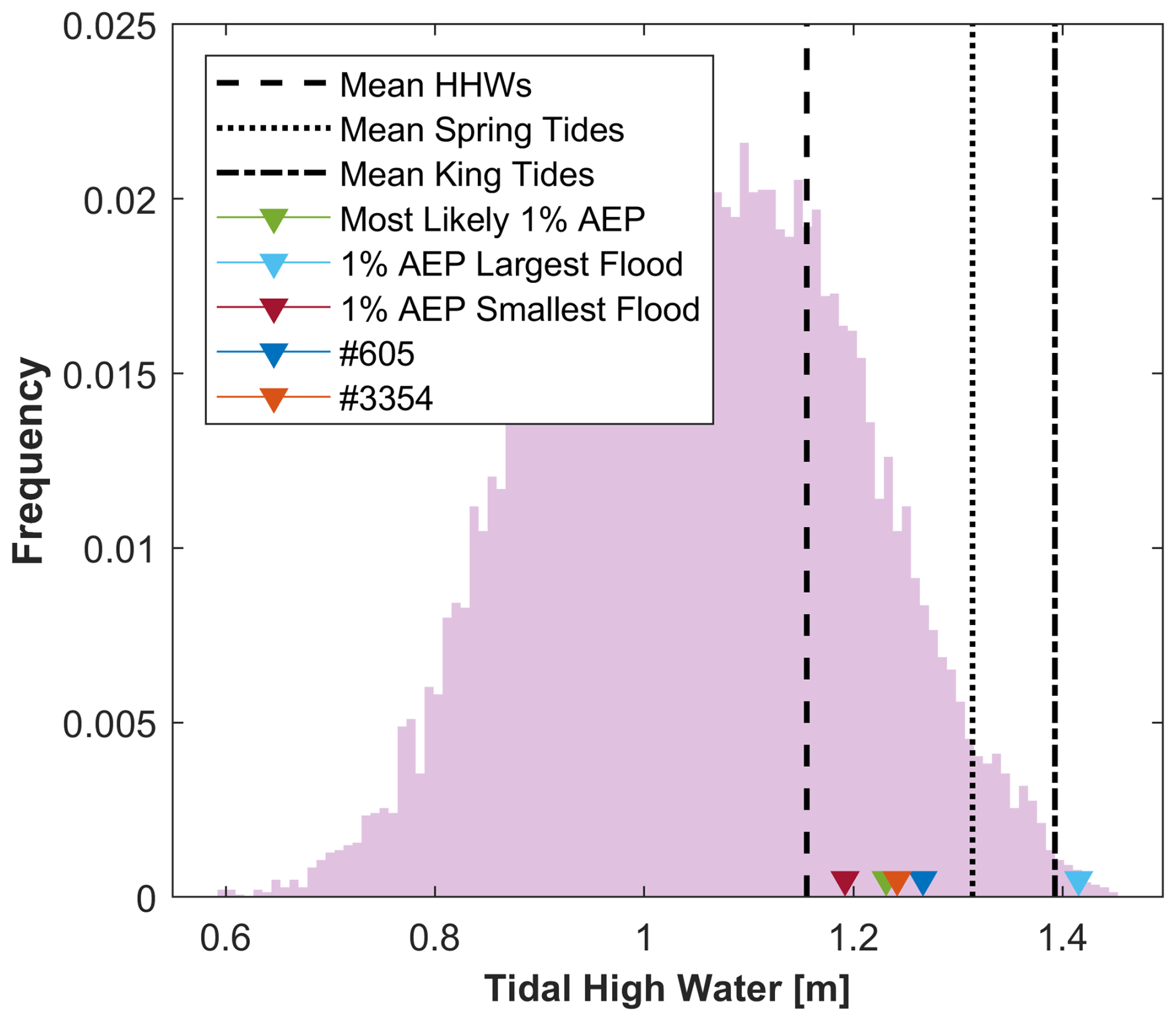
Figure 3 Histogram of tidal high water levels over the last 19 year period from 2003 to 2021. Black lines show the tidal levels of MHHW, Mean Spring Tide, and Mean King Tide (defined as the largest annual tide). Coloured lines show as an example the largest high tide levels of the tidal curves selected for the synthetic events shown in Fig. 2b–d, and two additional synthetic events (#605 and #3354) discussed in the results section. Tidal levels are referenced to NAV 88 datum.

3.2 Flood Model

We use the dynamic flood model SFINCS (Super-Fast INundation of CoastS), which was designed specifically for simulating flooding from multiple flood drivers (Leijnse et al., 2021), since we are interested in capturing interactions between rainfall and coastal water levels as well as the effects of spatio-temporal variability of compound events on the flood response. SFINCS is a reduced-complexity flood model that balances computational efficiency with accuracy, making it a perfect candidate to simulate thousands of events at a reduced computational cost.

The municipality of Gloucester City is encircled by the catchments of Newtown Creek and Little Timber Creek, for both of which discharge data is unavailable. Therefore, we define the SFINCS model domain (Fig. 1) to cover the catchments of these two creeks by their 14-digit hydrologic units from the NJDEP Bureau of GIS (New Jersey Department of Environmental Protection, Bureau of Geographic Information Systems, 2021; Table S1 in the Supplement). This domain encompasses all runoff that could potentially lead to pluvial flooding in the study area or fluvial flooding from the creeks. We define an open boundary along the Delaware River where the water level boundary conditions are given. The inland boundaries of the model domain are defined as “outflow” to allow any water flow to exit the domain. We use the subgrid approach of SFINCS with a dual resolution of 10 m (758 904 cells) and 1 m (147 450 698 cells) and the Digital Elevation Model (DEM) of Coastal National Elevation Database (CoNED) from the U.S. Geological Survey (U.S. Geological Survey, Earth Resources Observation and Science (EROS) Center, 2018; Fig. S1), which has a horizontal resolution of 1 m and a vertical accuracy of 10 cm (Danielson et al., 2016). This DEM at 1 m is aggregated using the median to 10 m in ArcGIS pro-3.2.0. We use spatially varying surface roughness based on land cover data from the NJDEP Bureau of GIS (Table S1), converting land classifications into Manning's coefficients based on guidance from the U.S. Army Corps of Engineers (USACE, 2021). Water level boundary conditions are provided as time series at the location of the Philadelphia tide-gauge and the model interpolates them along the open boundary of the Delaware River. Rainfall forcing is applied as spatially varying fields, with the same resolution as the AORC data (Fig. 1); SFINCS interpolates these onto the model grid resolution. The model is run with the advection term neglected, solving the local inertia equations. We use the GPU version of SFINCS and run the 5000 simulations on an Intel(R) Core (TM) i7-13700KF CPU and NVIDIA GeForce RTX 4080 GPU. The outputs of the simulations at 10 m resolution are downscaled to 1 m resolution using MATLAB 2023a.

Validation and calibration of flood models is a difficult task due to the common lack of observed flood data worldwide (Merz et al., 2024; Molinari et al., 2019). This is especially true for under-resourced regions; but the lack of observed flood data is also an issue in developed countries and more noticeable in the case of pluvial flood events, which are the most frequent in our study area of Gloucester City (Hino and Nance, 2021).

To address the challenges of flood model validation in data-scarce environments, we conducted an extensive search for observational data in Gloucester City. We evaluated a wide range of sources, including satellite imagery, high-water marks, FEMA reports, NOAA's Storm Events database, local news articles, and crowd-sourced platforms such as MyCoast and Twitter. Although conventional data sources provided limited information, we identified and simulated three documented flood events (2009, 2019, and 2020) for model validation. As part of this process, we evaluated the model outputs when including infiltration, finding an overestimation of infiltration and underprediction of flooding using the Curve Number method. Based on this and the high imperviousness of the urban area, infiltration was excluded from the final model configuration. Additionally, the known flood-prone areas identified by local authorities (Smith, 2023) were well captured by our 10-year flood hazard map. This multi-source approach provides the most robust validation feasible for this site given current data availability. A detailed description of the model validation is included in the Supplement.

4 Results

4.1 Differences in flood response from events with the same (joint) probability

We simulate flooding from 25 events with a 1 % AEP (1 % chance of occurring in any given year) that have different combinations of the magnitude of rainfall and NTR peak, but also different temporal and spatial evolutions and are combined with different tidal curves (Fig. 2). We find that the floodplain of each of these 1 % AEP events is different (Fig. S6), resulting in very large differences in both flood extent and depth between some of the events (Fig. S6). In Fig. 4a, we show the frequency of flooding at each cell (1 m²) from all 25 1 % AEP events; a frequency of 1 indicates that the particular area is flooded from all 25 events and a frequency near zero indicates that this area is only flooded from one or few of the 25 events. Certain areas scattered throughout the municipality experience flooding during all events with a 1 % chance of occurring in any given year (1 % AEP; green areas in Fig. 4a). However, a larger area is flooded only by a few of these events, which shows that selecting only one event with 1 % AEP for estimating flood hazard can introduce large uncertainties in exposure (and subsequently risk). Areas flooded only from a few 1 % AEP events are mainly along the Delaware River and creeks, where both flood drivers interact. In contrast, pluvial hot spots, i.e. regions that are not hydrologically connected to the Delaware River or creeks and thus rainfall is the only flood driver, exhibit notably less variability in flood extents and water depths between the different events of 1 % AEP. The variability of flooding in pluvial hotspots is more clearly observed by comparing the flood hazard maps across the 25 events presented in Fig. S6.

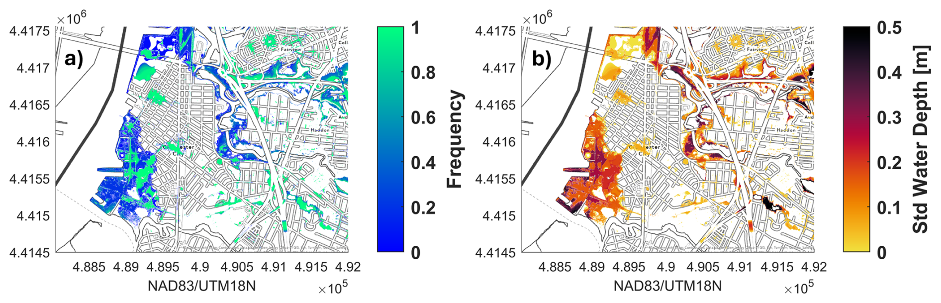
Figure 4 (a) Frequency of flooding at each model cell (1 m²) from the 25 events selected along the 100-year (1 % AEP) isoline. (b) The standard deviation of water depth (m) at each model cell (1 m²) between the 25 events selected along the 100-year (1 % AEP) isoline [NAD83/UTM18N. Source: Esri | Powered by Esri].

We also analyze the variability in water depths using the standard deviation between the flooding from all 25 events of 1 % AEP in all model cells (Fig. 4b). Larger standard deviations in water depth exist in regions where all events of 1 % AEP produce flooding, with maximum values of ∼0.8 m. Larger variability of water depths also exists in coastal regions, where both flood drivers interact, while small variations occur in pluvial hotspots (see also Fig. S6).

The largest and smallest flooding, in terms of flood extent and volumes, are produced by events that have almost the same 18 h accumulation rainfall and NTR peak, 59.18 mm and 1.86 m and 57.18 mm and 1.88 m respectively, and thus lie very close to each other on the 100-year (1 % AEP) isoline (Fig. 2c and d). However, the NTR hydrographs of these events are different, with one of them lasting for several hours with sustained large water levels (Fig. 2c) while the other is shorter and with lower water levels (Fig. 2d). In addition, the two events are combined with different tidal curves with high-tide levels that differ by more than 20 cm, an average MHHW and a larger than average king tide (see Fig. 3). The 1 % AEP event that produces the smallest flooding is combined with a tidal curve with high-tide levels similar to MHHW, but the 1 % AEP event that generates the largest flood is combined with a tidal curve that reaches values larger than the average king tide (Fig. 3). These factors cause the water level hydrographs of these events to differ in their temporal evolution and to have water level peaks that differ by ∼0.5 m, which combined leads to the large differences in flood response. Although the tidal curve combined with the 1 % AEP event that produces the largest flood might appear “extreme”, the analysis of the long-term modulations of the tide reveals that this king tide level was reached several years earlier in the current nodal cycle (Fig. 5). By extending the fitted long-term modulation, we show that the tides are currently in the ascending phase of both nodal and perigean cycles, with a peak expected in 2026. As a result, the likelihood of the tidal level of this particular synthetic event is higher over the coming years.

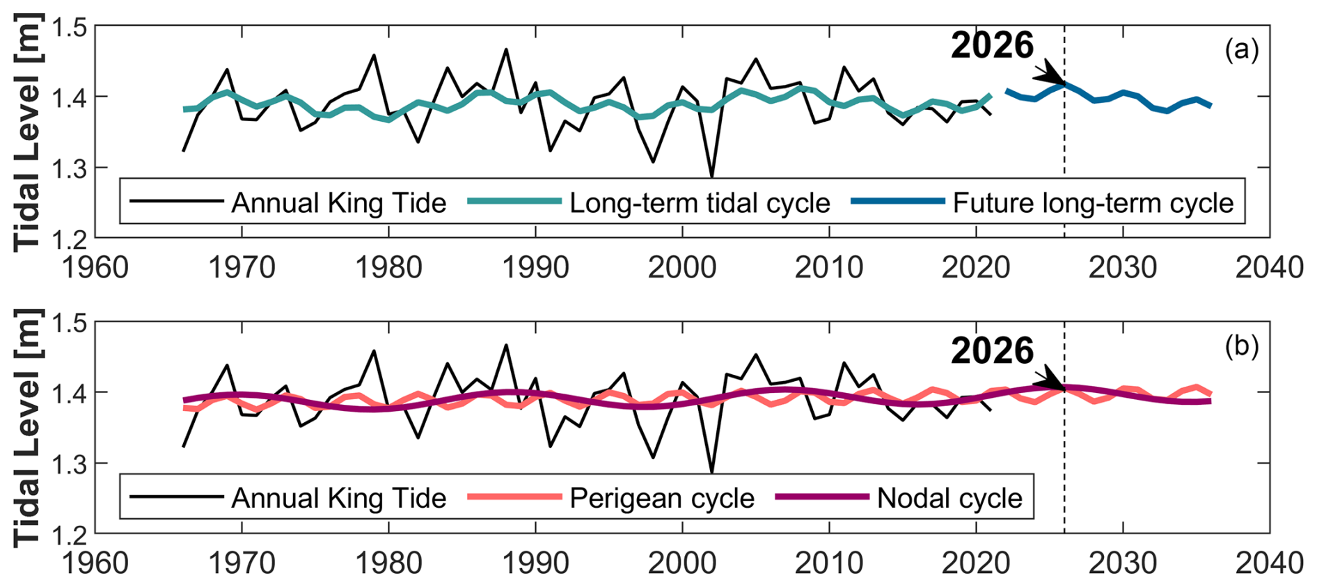
Figure 5 Annual king tide levels (as the maximum tidal level) at the tide-gauge of Philadelphia used in this study. Estimated long-term variability of king tides (a) from the combined nodal (18.6-year) and perigean (4.4-year) cycles including prediction of future combined peak of these long-term cycles expected for 2026; (b) separated nodal (18.6-year) and perigean (4.4-year) cycles for the historical and future period. Tidal levels are referenced to NAV 88 datum.

These results show that the variability of the NTR hydrograph, together with the variability of the tidal curve, have very large effects on the resulting flooding since events with almost equal NTR peaks can produce very different flooding. The topography also plays an important role (Fig. S1); when the water level at the Delaware River boundary exceeds the elevation of the coastline, the large low-lying region behind it floods. Thus, small increases in water levels along the hydrograph can cause large changes in flood extents when certain thresholds are exceeded.

We also compare the flooding arising from all events with a 1 % AEP with the “most likely” event (i.e. “design event”) in order to assess the uncertainties related to the use of a single design event when assessing flood hazards. This is commonly done when following the event-based approach for compound flood hazard modeling. In terms of flood extent and volumes (Fig. 6), most of the events with a 1 % AEP (17 and 19 of the 25, respectively) produce larger flooding than the “most likely” design event. However, there are substantial spatial variations between events, as some can produce larger flooding in some areas and smaller flooding in other areas (not shown). We calculate the total flood extent and volume of all 5000 events to estimate the empirical return periods of these two flood metrics (Fig. 7). Based on the empirical distribution, the “most likely” event has a return period of 38 years in terms of extent and 33 years in terms of total flood volume. 20 of the events with 1 % chance of happening in any given year have return periods <100 years (>1 % AEP, >1 % chance of happening in any given year) in terms of total flood extent, while only 12 events have return periods <100 years in terms of total flood volumes. This shows that using a single design event when assessing compound flood hazards can lead to large uncertainties in both flood extent and depth, often resulting in an underestimation of the extent in our case study.

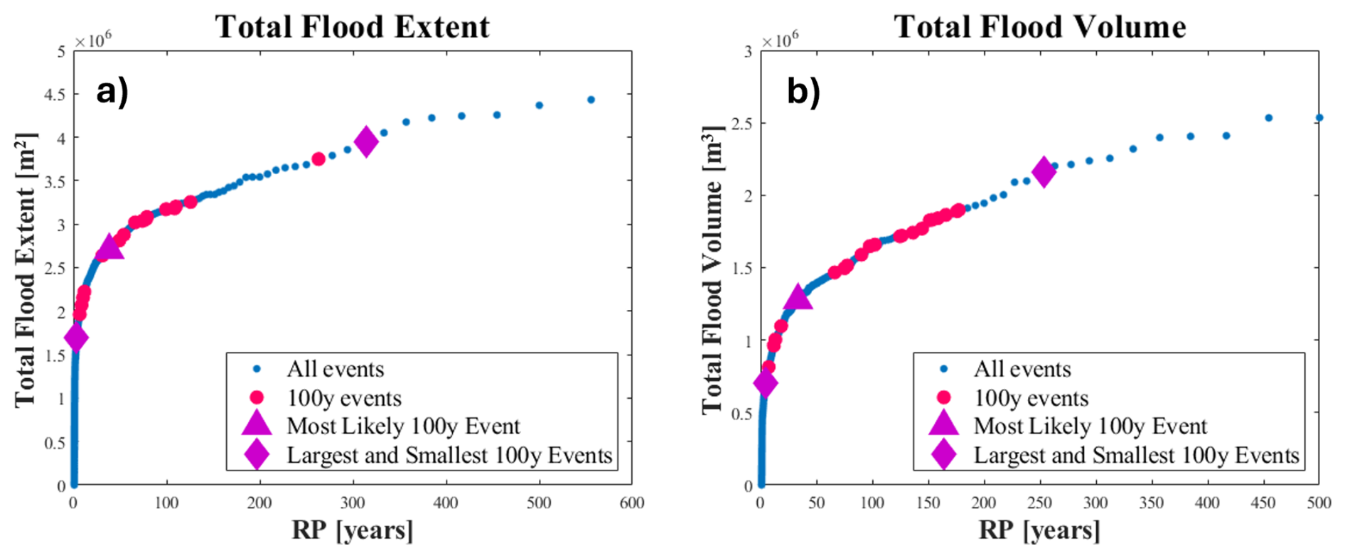
Figure 6 (a) Empirical distribution of total flood extent from all events (blue points), 1 % AEP events (pink dots) including the “most likely” (purple triangle) and largest and smallest flood (purple diamonds); (b) same as (a) but in terms of total flood volumes.

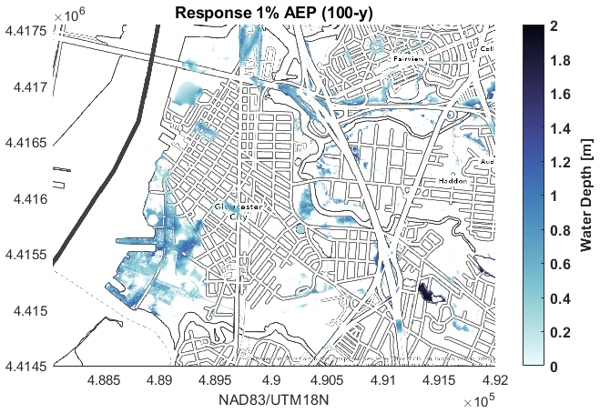
Figure 7 1 % AEP response flood hazard map calculated by the empirical distribution of water depths from 5000 simulations; we show the 1 % AEP water depth at each model cell (1 m²) [NAD83/UTM18N. Source: Esri | Powered by Esri].

4.2 Response-based flood hazard

We estimate the response-based flood hazard map by calculating the empirical distributions of water depths at each model cell (of 1 m²) and show the water depth with a 1 % chance of happening in any given year (1 % AEP; Fig. 6). This 1 % AEP response flood hazard can thus be produced by different events in different regions. Comparing the response flood hazard to the flood hazard of the different events with a 1 % AEP, the response flood hazard has generally larger flood extents and water depths, with a few exceptions. In the 1 % AEP response flood hazard map, there is a larger area in the south of Gloucester City facing the Delaware River (Fig. 6) with water depths up to 1 m. However, this region is only flooded by a few of the events with a 1 % 1 % AEP (Fig. 4). In contrast, the flood hazard in the northern Delaware region from the response-based flood hazard map is similar to the region flooded by all the events with a 1 % AEP. In this region, the event with a 1 % AEP that causes the largest overall flooding (Fig. 2c) also produces more extensive flooding. This might be caused by the relatively longer hydrograph of that event combined with a larger-than-average king tide. Comparing the differences between the response-based and event-based flood hazard in the pluvial hotspots (areas not hydrologically connected to the Delaware River), only one of the events with a 1 % AEP causes larger flooding than the response-based approach. In the northeast region of the domain, ten of the events with a 1% AEP (1 % chance of happening in any given year) produce larger flooding than the response-based 1 % AEP floodplain. This can point to effects of the spatial variability of rainfall fields between events, which are masked in the joint probabilities because these are based on the 18 h accumulated average rainfall in the catchment.

We trace the events that produce the response-based flood hazard of 1 % AEP and group them by their corresponding return periods based on the joint probabilities of flood drivers (Fig. 8). This helps identifying the types of events causing the 1 % AEP water depth in different areas of our study site. Across most of the study domain, and especially in the urbanized region in the centre of the city, events with joint AEPs much higher than 1 % can lead to the 1 % AEP water depth as identified from the response-based approach. Most of the water depths with a 1 % AEP along the south coastal region of the city are produced by a single compound event with a ∼50 % AEP (50 % chance of happening in any given year or 2-year return period; yellow) and another event with a ∼7 % AEP (7 % chance of happening in any given year or 14-year return period; light orange) based on the joint probability distribution of NTR and 18 h accumulated rainfall. Although the NTR peak of these events is around 1 m, and thus much smaller than other events, these two events have long hydrographs with sustained water levels for several hours and combined with tidal levels of around 1 m can produce the 1 % AEP water depths in that area (Fig. S7). The tidal levels of these two events (#605 and #3354 in Fig. 3) exceed the MHHW but remain below the mean spring tides, making them likely to occur on a fortnightly basis. The 1 % AEP water depths in regions that are only affected by pluvial flood events are generally also caused by events with >2 % AEPs. Notably, there are two pluvial hotspots in the city region produced by events with >10 % chance of happening in any given year (less than 10-year return period or >10 % AEPs). These are produced by two different events, both with AEPs of ∼12 % based on the joint probability distribution. More detailed assessment of the rainfall fields of these events reveals that they have larger rainfall over that area of the model domain, which gets masked when averaging the rainfall over the entire catchment (Figs. S8–S9).

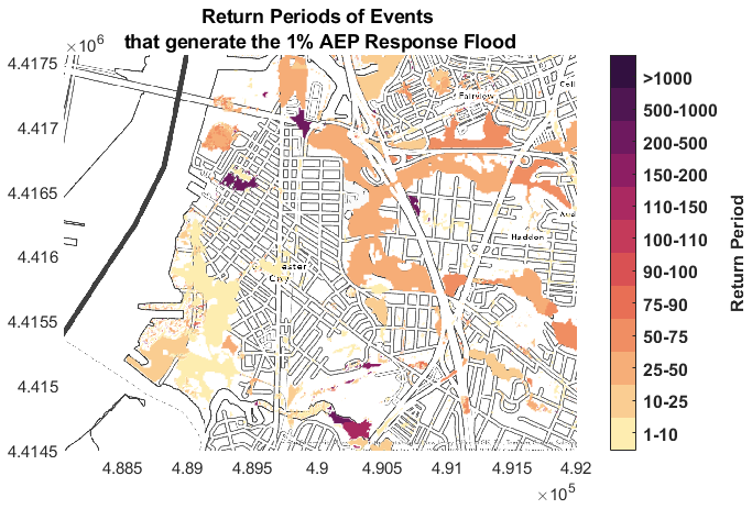
Figure 8 Return periods (based on the bivariate extreme model) of the events that generate the 100-year water depth from the response approach [NAD83/UTM18N. Source: Esri | Powered by Esri].

5 Discussion

Much of the research has been dedicated to improving extreme statistics of compound events and to quantifying the uncertainties of extreme value analysis of flood drivers (e.g., Lucey and Gallien, 2024), assuming that the probability of the event approximates the probability of the resulting flooding. However, little research has been focused on analyzing the latter, specifically for compound flooding, in which more than one driver is involved, and thus different combinations of flood driver magnitudes have the same joint probabilities. Here, we have assessed how linear is the relationship between the probability of the event and the probability of flooding for a case study in Gloucester City (NJ, U.S.) by comparing the flood hazard with a 1 % AEP (1 % chance of happening in any given year) based on the event- and response-based approaches. We find that the 1 % AEP water depth can be produced by different events in different parts of the city and that the AEPs of these events are often much larger than 1 %. This means that the relationship between the probability of the event and the probability of flooding does not follow a one-to-one relationship. These results are in line with previous studies that addressed the same question for rainfall-driven flooding (Baer, 2025; Perez et al., 2024; Winter et al., 2020). We find that the region of Gloucester City with the largest 1 % AEP flood hazard is the coastal zone and it is caused by events with >5 % chance of happening in any given year (>5 % AEP and less than 20-year return period) based on the joint probability distribution of 18 h rainfall accumulation and NTR peaks. However, these events (Fig. S7) exhibit sustained high NTR levels, which, when combined with tidal levels larger than MHHW, can result in greater water depths than most of the analyzed events with 1 % chance of happening in any given year (1 % AEP). Similarly, the regions impacted mainly by pluvial flooding also tend to experience the 1 % AEP water depths from events with >10 % AEP (>10 % chance of happening in any given year or less than 10-year return period). In this case, the events producing the 1 % AEP water depths in the city show spatial variations in their rainfall fields, with larger precipitation rates over the urbanized city region. However, the spatial variability of the rainfall fields is smoothed when calculating the average rainfall in the catchment to perform the extreme value analysis, and together with small NTR peaks, these events get assigned high AEP values (or short return periods).

These results show that the response-based approach leads to better representation of flood hazard at the household level. It accounts for the temporal variability of NTR hydrographs, combination with tides and mean sea level, and the spatial variability of rainfall fields. All of those are not explicitly accounted for in extreme value models to derive joint AEPs or joint return periods for the event-based approach. Nevertheless, some applications, such as emergency management, might need event-based flood hazard maps.

Event-based flood assessments commonly use a single design event with specific temporal and spatial structure, thus neglecting the variability in the temporal and spatial evolution of the flood drivers between different events. We have shown that using a single design event with a 1 % chance of happening in any given year (1 % AEP) can introduce large uncertainties in both flood extents and water depths that arise from the different combinations of the drivers' magnitude but are mostly due to differences in temporal and spatial evolution between events. Events of almost equal magnitude but different spatial rainfall fields and temporal distribution of the water level hydrographs can produce very different flood extents and water depths. The disparities in resulting flooding are more pronounced in the coastal areas of our study domain, where both flood drivers interact and are further influenced by changes in tidal variability. Considering the variability of the tide, rather than relying on a single MHHW level is also crucial, as tidal fluctuations over longer time scales (such as spring and king tides) can influence coastal flooding. This is especially relevant now, as tides are in the ascending phase of their long-term cycles, which are projected to reach their peaks within this decade, with the first peak expected as soon as 2026 at our study site. This finding highlights the necessity of taking into account the variability in the tidal levels.

Ignoring the variability in the spatio-temporal structure between extreme events by relying on a single design event can lead to significant uncertainties in flood exposure, which in turn can result in substantial uncertainties in flood risks. One way to address this limitation when using the event-based approach is to employ ensembles of events that account for variations in the spatial and temporal structure of the flood drivers. From that one can produce an ensemble of flood hazard maps for a desired return period, similar to probabilistic flood maps but for a given AEP (or return period).

Our study has several limitations that highlight areas for further research. We focused on a small study site with a particular topography that is affected by two flood drivers with associated variabilities. Thus, the results cannot be extrapolated to other coastal regions. However, we expect that our general conclusions are transferable to other regions. For example, the importance of temporal and spatial variations of the flood drivers has been pointed out by other studies in Germany (Kupfer et al., 2024; Santamaria-Aguilar et al., 2017) and in the UK (Quinn et al., 2014), showing that changes in water level hydrographs can produce large changes in flood hazards. Likewise, differences in rainfall-induced flooding between the event-based approach and the use of synthetic storms that capture the temporal and spatial variability of rainfall fields between events have been shown to significantly influence flood hazard estimates in the East and Gulf coasts of the US (Baer, 2025; Perez et al., 2024) and Austria (Winter et al., 2020). Another limitation of our study is that we use a synthetic event set developed using a data-driven statistical framework, which is limited to observed events. Although the statistical framework used to generate the synthetic events account for more dependencies between parameters that characterize the events (e.g. time lags) than other previous frameworks (Couasnon et al., 2018; Moftakhari et al., 2019), it may not fully capture the full range of the potential spatio-temporal variability of flood drivers. Tropical cyclones might also be underrepresented in the historical sample since their frequency of occurrence is very low. This limitation can be overcome by using synthetic tropical cyclones that are dynamically downscaled to the study site (e.g., Gori et al., 2020) Methods such as the JPM, which expand the storm climatology, enable the generation of a larger set of tropical cyclones, and capture greater variability in their spatio-temporal characteristics compared to historical records. However, these methods are computationally demanding, as flood drivers must be generated in advance of the flood assessment using hydrodynamic models (see e.g. Bartlett et al., 2025; Gori and Lin, 2022; Grimley et al., 2025). Further research is needed to evaluate how different synthetic event generation approaches affect flood hazard estimates. Given the high computational demands of JPM, its application across large coastal areas may be impractical, making data-driven approaches like the one used in this study a more efficient alternative. Similarly, other data-driven techniques, such as stochastic storm transposition, are increasingly being adopted to generate synthetic rainfall fields for assessing rainfall-driven flood hazards (Baer, 2025; Lehman, 2023; Perez et al., 2024; Winter et al., 2020). However, further investigation is needed to ensure that this method adequately preserves the interdependencies between coastal and rainfall processes when generating synthetic compound events for coastal flood assessments. A potential source of uncertainty in the variability captured by our synthetic event set arises from not disaggregating river- and coastal-driven components of the NTR. In our mid-estuarine study area, both processes contribute to the NTR, along with their nonlinear interactions. Separating these contributions would introduce considerable complexity due to their tightly coupled dynamics. Our approach is supported by recent work from McKeon and Piecuch (2025), who investigated the relative influence of coastal and fluvial drivers in the Delaware Estuary above flood thresholds. They found that most events observed at the Philadelphia tide gauge were primarily driven by coastal processes (e.g., tides and storm surge), but others resulted from river discharge alone or a combination of both mechanisms. Another limitation of the synthetic event set used is the reliance on mathematically defined thresholds for event selection, rather than thresholds based on actual flood impacts. This approach may exclude relatively frequent, lower-magnitude events that fall outside the statistical tails of the drivers' distributions but are still capable of causing localized flooding, potentially influencing response-based flood estimates. In our study, we evaluated the flood response of events near the selected thresholds and found that several produced no flooding, while others resulted in only minor inundation, with empirical return periods between 1 and 2.8 years. As a result, the selected thresholds did not affect our response-based flood estimates; however, this may not hold true in other regions with different hydrologic or exposure characteristics.

Our flood model approach also has some limitations. First, we are neglecting the stormwater system and thus we might overestimate flooding and neglect the fact that some areas might experience flooding due to backwater effects in the system. Stormwater systems are typically designed for events with low to moderate return periods (often the 10-year event, or 10 % AEP event) while we have focused on the 1 % AEP (100-year) flood hazard. Such events would likely exceed the capacity of the stormwater system. Nevertheless, the exclusion of stormwater infrastructure may have a greater impact on the results for smaller, more frequent events, potentially leading to an overestimation of flooding in cases where the existing drainage system would likely manage the runoff. However, this should not affect the response-based estimates for the 1 % AEP since the empirical distribution will not change for rare large events. In addition, we neglected infiltration based on the validation of the model for one single event for which we have information on reported flooding at a single location. Although most of our study domain is urban and thus covered by impervious surfaces, we might underestimate infiltration in areas with larger amounts of vegetation such as areas around the creeks. The bathymetry of the creeks might also not be very accurately represented in the CoNED DEM used (Fig. S1). The limited depth representation of creek channels, combined with the exclusion of infiltration processes, likely results in an overestimation of floodwater depths along the margins of the creeks. Both the validation of the flood model and calibration of parameters and processes such as infiltration can be improved if more observed flood data from past events is available. The lack of this data is a common problem worldwide (Merz et al., 2024; Molinari et al., 2019) and it can be overcome by systematically collecting flood data after flood events or making available datasets such as claims from the National Flood Insurance Program (Sebastian et al., 2021).

6 Conclusions

Coastal communities are experiencing growing flood hazards due to rising sea levels, more frequent extreme events, and an increase in population and assets in flood prone areas. Consequently, more robust flood hazard estimates are required to develop effective adaptation strategies to mitigate flood impacts. Although significant attention has been focused on reducing uncertainties in the estimation of probabilities of flood drivers, little is known about how well the probability of compound events approximates the probability of flooding. Here, we addressed this issue by comparing flood hazard derived from the event- and response-based approaches for a case study in Gloucester City (NJ, U.S.), which is frequently affected by pluvial and coastal flooding.

Our findings reveal that the 1 % AEP flood hazard derived from the response-based approach can be caused by different events in various parts of the city, with AEPs much larger than 1 % (return periods <100-year). In the coastal area, events with >5 % chance of occurring in any given year (>5 % AEP or less than 20-year return period) can produce a 1 % AEP water depth if the NTR hydrograph leads to prolonged high water levels when combined with tidal levels between the MHHW and average spring tides. In this context, our findings are in line with previous studies that highlighted that the long-term variability of tides can modulate both minor and extreme flooding (Enriquez et al., 2022; Thompson et al., 2021). We find that considering tidal variability is crucial, rather than relying on the assumption of a constant MHHW, as flooding from both low and high return period events can differ substantially depending on the tidal level considered. Tides are currently in the ascending phase of the nodal and perigean cycles, which are expected to peak in 2026 in our study region, making it more likely that storm surges coincide with high tide levels, thus increasing the probability of flooding. Similarly, not accounting for the variability in the spatial pattern of rainfall fields between events, which is masked when using catchment average values for extreme value analysis, can underestimate pluvial flood hazards. This study highlights the importance of considering the variability of the temporal and spatial structure of extreme events in flood hazard estimates. The traditional method of using a single design event in event-based assessments can lead to considerable uncertainties in flood extent and water depth, especially due to varying combinations of flood drivers. The response-based approach, which accounts for factors like tidal variations and the full range of the variability of temporal and spatial distributions at event scale, provides a more robust representation of flood hazards. However, event-based maps remain essential for some applications such as emergency management. Using ensembles of events that account for these variations would enhance flood hazard estimates derived from the event-based approach.

While our results are not directly applicable to other regions, we expect similar conclusions elsewhere regarding the impacts on compound flood hazards from neglecting the temporal and spatial variability of flood drivers. Future work should focus on producing more robust flood hazard estimates by using many compound events including their temporal and spatial evolution rather than focusing on single design events for given AEPs or return periods. Similarly, future projections of flood hazards should also account for potential changes in the temporal and spatial evolution of events rather than focusing only on changes in their magnitude. Additionally, future research should aim to evaluate how different methods for generating synthetic events influence the resulting flood hazard estimates. Such comparisons can help inform best practices for generating more reliable flood hazard assessments under both current and future climate conditions.