Indirect costs of floods: a case study of highways road users

Hydrometeorological events have a significant impact on road infrastructure and traffic flow. Floods can collapse or weaken bridges, compromise river protection, and flood riverine roads, restricting or halting the traffic. These events incur additional user costs owing to increased travel times from the rerouting and reduced speeds on affected roads. The economic impact of such events on road networks is typically quantified in terms of infrastructure recovery costs, while the expected user cost (EUC) of driving on damaged roads is often neglected. This study estimates flood risk to road networks by integrating a hydrological-hydraulic model with road and bridge vulnerability assessments and traffic assignment models to calculate the EUC. The procedure was applied to the Aconcagua River basin in central Chile, considering floods with return periods ranging from 2 to 100 years, bridges vulnerability to scour, road waterlogging, travel times, and fuel consumption costs. In the 100-year scenario, 7.65 km of roads and 3 bridges were affected. Considering all analysed return periods, the EUC of the network reached USD 5.7 × 10⁶ yr⁻¹. These results provide a quantitative basis for flood risk management and support decision-making regarding prioritization of road and bridge interventions in the Aconcagua River basin.

1 Introduction

Hydrometeorological events (HME) originate from atmospheric and meteorological events that result in storms, droughts, heat waves, and floods that modify territory over time and affect the subsistence of people and infrastructure (Sahani et al., 2019). Floods are primarily caused by rainfall and, in mountain watersheds, by rapid snowmelt, which increases river discharge, submerges lowland areas, and generates surface runoff that affects the built environment. Floods recurrently affect road networks and their infrastructure, causing the total or partial destruction of road segments and bridges, and consequently reducing the physical and operational road network performance during and after the event. Floods can cause bridges to collapse or weaken river protection. In some areas, riverine roads may be flooded. Furthermore, flood-scour bridge foundations affect their structural integrity and prevent vehicular traffic (Klinga and Alipour, 2015; Hung and Yau, 2017). Furthermore, road waterlogging reduces traffic speed or prevents passage depending on the water height over the road (Pregnolato et al., 2017b; Contreras-Jara et al., 2018). In these cases, the impact on road network performance related to travel time increases because of reduced speed and traffic rerouting. The indirect impacts of non-travel decisions can also reduce the traffic level on the network and induce an alternative cost per non-travel decision. Both impacts involve road users and, depending on the level of damage to the highway network, can be extended during the planning and delivery of repairs for damaged infrastructure.

The impact of floods on road network users depends on the magnitude of the HME, infrastructure vulnerability and exposure, and traffic distribution over the affected road network, making it important to estimate the flood risk on roads and bridges. Risk comprises the events that may occur, their consequences and the associated probabilities, with severity characterizing the consequences, commonly expressed as monetary losses (Aven, 2011). Risk analysis in road networks therefore focuses on calculating economic losses in terms of the recovery costs of physical infrastructure. By contrast, economic loss estimation does not always consider road asset fragility or costs incurred by road users. This aspect has drawn interest in risk assessment literature in recent years (Lam and Adey, 2016; Hackl et al., 2018; Zhang and Alipour, 2019 and 2020; Wang et al., 2020).

Flood risk is the probability of damage to infrastructure over a certain period in interaction with its physical vulnerability and exposure and associated economic losses (Merz et al., 2009; Tsakiris, 2014). This is expressed in terms of the expected annual damage caused by floods during the return period (Penning-Rowsell and Green, 2000).

Flood risk modeling of road networks under this approach includes four general steps: (1) hydrological and hydraulic modeling, (2) road asset vulnerability, (3) traffic assignment modeling under normal and damaged conditions, and (4) economic loss estimation. Wisetjindawat et al. (2017) identified the following hydrological modeling approaches: direct flow measurements, remote rainfall and flood perception, rainfall-runoff modeling, and post-event measurements. Arseni et al. (2020) used flow station data for hydrological modeling, which is appropriate if there are sufficient fluviometric stations and data per station to model watersheds or sub-watersheds. Wang et al. (2020) used non-global climate models to model the surface runoff. Vincendon et al. (2016) used hydrological balance-based models to predict flood flow. Hydraulic modeling procedures do not differ significantly and generally use digital elevation models combined with hydrodynamic, one-dimensional (1D), two-dimensional (2D), and ad hoc models. Teng et al. (2017) provided a detailed description of the available hydraulic models. Vulnerability represents the susceptibility of the receiver bodies to damage caused by natural or anthropogenic events (Menoni et al., 2012). Physical vulnerability represents the damage susceptibility of physical assets such as roads, bridges, and cut slopes, which are commonly induced by natural events (Berdica, 2002). This susceptibility is represented by fragility or damage probability models, which estimate the probability of reaching a particular damage state. Each asset has a unique fragility curve for a specific event (Hackl et al., 2018). Traffic assignment modeling determines the travel time and operating speed under normal and damaged road network conditions. Consequently, user costs can be estimated in terms of travel time and additional fuel consumption costs due to rerouting. The Beckmann et al. (1955) model and its updates are frequently used to estimate travel time in road networks in combination with traffic assignment models, assuming no congestion and origin-destination matrices (Hackl et al., 2018). Zhang and Alipour (2019, 2020) used this approach for traffic modeling in flood risk assessments.

Generally, flood risk is estimated in terms of the return period without considering the direct or indirect costs to people and their economic activities. Flood effects can be estimated economically; for instance, agricultural and housing losses or the costs of evacuation and attending to the people affected are commonly considered direct costs. In contrast, the effect of floods on highway infrastructure and the cost transferred to road users in terms of travel time increase and additional fuel consumption are not included in the economic loss models. Consequently, the total economic losses for different flood scenarios regarding the return periods were underestimated.

In this study, we estimated the road user costs for networks affected by floods. The procedure integrates the vulnerability models of bridges and roads, a locally calibrated rainfall-runoff model for uncontrolled watersheds, and a traffic assignment model. The procedure was applied to a road network 1823 km in length, located in the lower Aconcagua river basin in central Chile. The flood scenarios included return periods of 2, 10, 25, 50 and 100 years. The discharge was modeled using a rainfall-runoff model calibrated for Chile by Verni and King (1977). Flood maps were obtained by using the HEC-RAS 2D model for each return period. Road network exposure was determined by overlapping flood and road network maps to identify flooded road network sectors and bridges affected by scour.

The vulnerability of waterlogged roads was estimated using the traffic interruption model developed by Contreras-Jara et al. (2018).Bridge vulnerability was estimated using the scour probability model developed by Contreras-Jara et al. (2021). Traffic was obtained by combining the travel time model of Nie et al. (2004) with the numerical solution of a static traffic assignment problem implemented by Kumar (2019) under normal and damaged network conditions. Travel time and fuel consumption costs were estimated and combined with the estimated road and bridge vulnerabilities to obtain a proxy for the impact of floods on the road network in the lower Aconcagua River basin in terms of road user cost losses. Finally, the results, discussion, and conclusions are presented.

2 Flood risk in highways networks

2.1 Quantification of flood risk

Following the definition given in Sect. 1, flood risk comprises the flood events considered, their consequences and the associated probabilities (Aven, 2011; Kron, 2005). Consequences comprise three factors (Gouldby and Samuels, 2005): exposure, vulnerability, and the potential affection on people or damage to infrastructures.

According to Hall et al. (2006), risk can be calculated using Eq. (1), where g(x) is the limit state function of a system with “x” characteristics, and I(.) is an indicator whose value is one if g(x)≤0; otherwise, it is zero. This implies that the system fails when g(x) is less than zero. The term f(x) is the probability density function that describes how the “x” system characteristics vary, and D(x) is the damage function of the system.

$$\begin{array}{}\text{(1)}& \text{Risk}=\int I\left(g\right(x)\le \mathrm{0})f\left(x\right)D\left(x\right)\mathrm{d}x\end{array}$$

A similar definition of risk was provided by Merz et al. (2009), who applied the expected annual damage (EAD) introduced by Penning-Rowsell and Green (2000) caused by floods. Flood risk is expressed by Eq. (2), where the decision variable is the water level (h), f(h) is the probability density function of the flood water level, and D(h) is the flood damage. There is a minimum water level value (h_d) at which the damage increases as the water level rises.

$$\begin{array}{}\text{(2)}& \text{Risk}=\underset{h_{\mathrm{d}}}{\overset{\mathrm{\infty }}{\int }}f\left(h\right)D\left(h\right)\mathrm{d}h\end{array}$$

Because flood scenarios are infrequent, Eq. (2) is expressed in discrete terms, as shown in Eq. (3) for the “m” probability increments and “j” intervals (Merz et al., 2009; Lugeri et al., 2010; Scorzini and Leopardi, 2017).

$$\begin{array}{}\text{(3)}& \begin{array}{rl}\text{Risk}& =\sum _{j=\mathrm{1}}^m\mathrm{\Delta }{P}_j{D}_j;D_j={\displaystyle \frac{\mathrm{1}}{\mathrm{2}}}\left[D\right(h{)}_j+D\left(h{)}_{j+\mathrm{1}}\right];\mathrm{\Delta }{P}_j\\ & =\left(P\right(h{)}_j-P\left(h{)}_{j+\mathrm{1}}\right)\end{array}\end{array}$$

where D_j is the average damage, and ΔP_j is the increment in the exceedance probability. Scorzini and Leopardi (2017), Arrighi et al. (2018), and Ziya and Safaie (2023) applied Eq. (3) Flood damage (D_i) is estimated using three return periods (T_i) to obtain Eq. (4).

$$\begin{array}{}\text{(4)}& \begin{array}{rl}\text{Risk}=& {\displaystyle \frac{\mathrm{1}}{T_{\mathrm{1}}}}\times D_{\mathrm{1}}+\left[{\displaystyle \frac{\mathrm{1}}{T_{\mathrm{2}}}}-{\displaystyle \frac{\mathrm{1}}{T_{\mathrm{1}}}}\right]\times {\displaystyle \frac{D_{\mathrm{1}}+D_{\mathrm{2}}}{\mathrm{2}}}\\ & +\left[{\displaystyle \frac{\mathrm{1}}{T_{\mathrm{3}}}}-{\displaystyle \frac{\mathrm{1}}{T_{\mathrm{2}}}}\right]\times {\displaystyle \frac{D_{\mathrm{2}}+D_{\mathrm{3}}}{\mathrm{2}}};\\ & \text{where }{T}_{\mathrm{1}}>T_{\mathrm{2}}>T_{\mathrm{3}}.\end{array}\end{array}$$

2.2 Flood risk in highway networks modeling

Bridges and road segments near rivers are exposed to flooding. Bridge foundations are affected by scouring, which weakens their structural resistance and limits heavy hauling vehicles and transit traffic. Under extreme conditions, a bridge can be closed, and consequently, traffic is diverted to other roads in the network. Flooded roads decrease vehicle driving speed and eventually interrupt traffic, forcing rerouting on the nearby roads. Owing to traffic rerouting, the total travel time and fuel consumption increase, resulting in higher road user costs. Engineers face challenges in estimating traffic reassignment, and road user costs increase as a proxy for the expected annual damage (EAD) in flooded highway networks (Pregnolato et al., 2017b; Hackl et al., 2018; Zhang and Alipour, 2019, 2020; Qiao et al., 2023; Rebally et al., 2026).

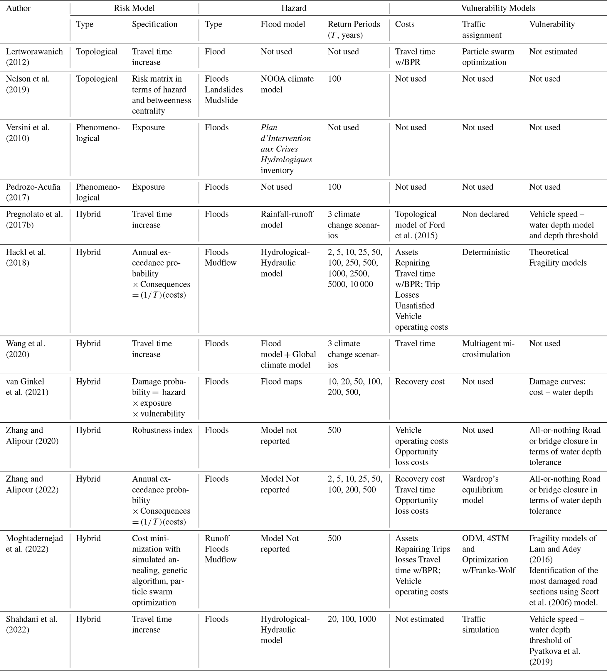
Table 1 summarizes the state-of-the-art of highway flood risk modeling. The flood risk has been studied using topological, phenomenological, and hybrid approaches. The topological approach identifies link interactions in the road network and the connectivity loss of a closed set of links and nodes (Lertworawanich, 2012; Nelson et al., 2019). This phenomenological approach uses climatic or hydrological-hydraulic models to identify flooded road network links and those that are potentially disabled (Pedrozo-Acuña et al., 2017; Versini et al., 2010). The hybrid approach integrates topological and phenomenological approaches, as well as traffic assignment modeling, to determine the user costs induced by floods in highway networks (Pregnolato et al., 2017b; Hackl et al., 2018; Wang et al., 2020; van Ginkel et al., 2021; Zhang and Alipour, 2020, 2022; Moghtadernejad et al., 2022; Shahdani et al., 2022; Papilloud et al., 2024). The hazard is thus modeled using common hydrological and hydraulic models and their variations, using return periods ranging between 2 and 50 years, and exceptionally up to 10 000 years.

Table 1 State of the art of flood risk models of highway networks. For each study, the table reports the risk modeling approach (type: topological, phenomenological, or hybrid, as defined in Sect. 2.2; Specification: the specific method used), the hazard characterization (type of hazard, flood model used, and return periods, T, considered), and whether the study incorporated road user costs, traffic assignment modeling, and infrastructure vulnerability assessment.

3 Methodology for estimating the road network flooding risk

3.1 General description of the procedure

The result of the procedure is economic losses in terms of costs for road users of road networks affected by floods for return periods between two and 100 years. To estimate the losses, the procedure incorporates hydrological and hydraulic modeling to simulate flood conditions, which then informs road and bridge vulnerability, culminating in a traffic assignment model that estimates the resultant economic impact.

Road vulnerability was estimated as a function of the probability of traffic interruption owing to flooding. Bridge vulnerability was calculated as the probability of scour exceedance. The exposure was obtained from overlapping flood maps and the road network under study. Flood maps were obtained using a combination of hydrological and hydraulic models for different return periods.

The indirect costs of flooding are estimated in terms of road user costs. These costs are the sum of fuel consumption and travel time costs. They were estimated under normal operating conditions of the road network and for restrained operations under different road flooding scenarios. Under normal conditions, road user costs are estimated by applying a traffic assignment model. The model assigns traffic to minimize the travel time of road users in an entire road network. Under restrained conditions, fuel consumption and travel time increase owing to rerouting caused by the disabling of total or partial road sectors and bridges or by speed reduction during the flood.

The traffic assignment model is applied to estimate the fuel consumption, travel time, and costs for different flood scenarios. The difference in fuel consumption and travel time costs between normal and restricted operations was the net increase in the cost of the entire road network for each flood scenario

3.2 Workflow

Figure 1 shows the step-by-step procedure proposed for road network risk estimation, which comprises (1) hazard modeling (HMH), (2) road network exposure (RE), and (3) road network risk calculation (RM).

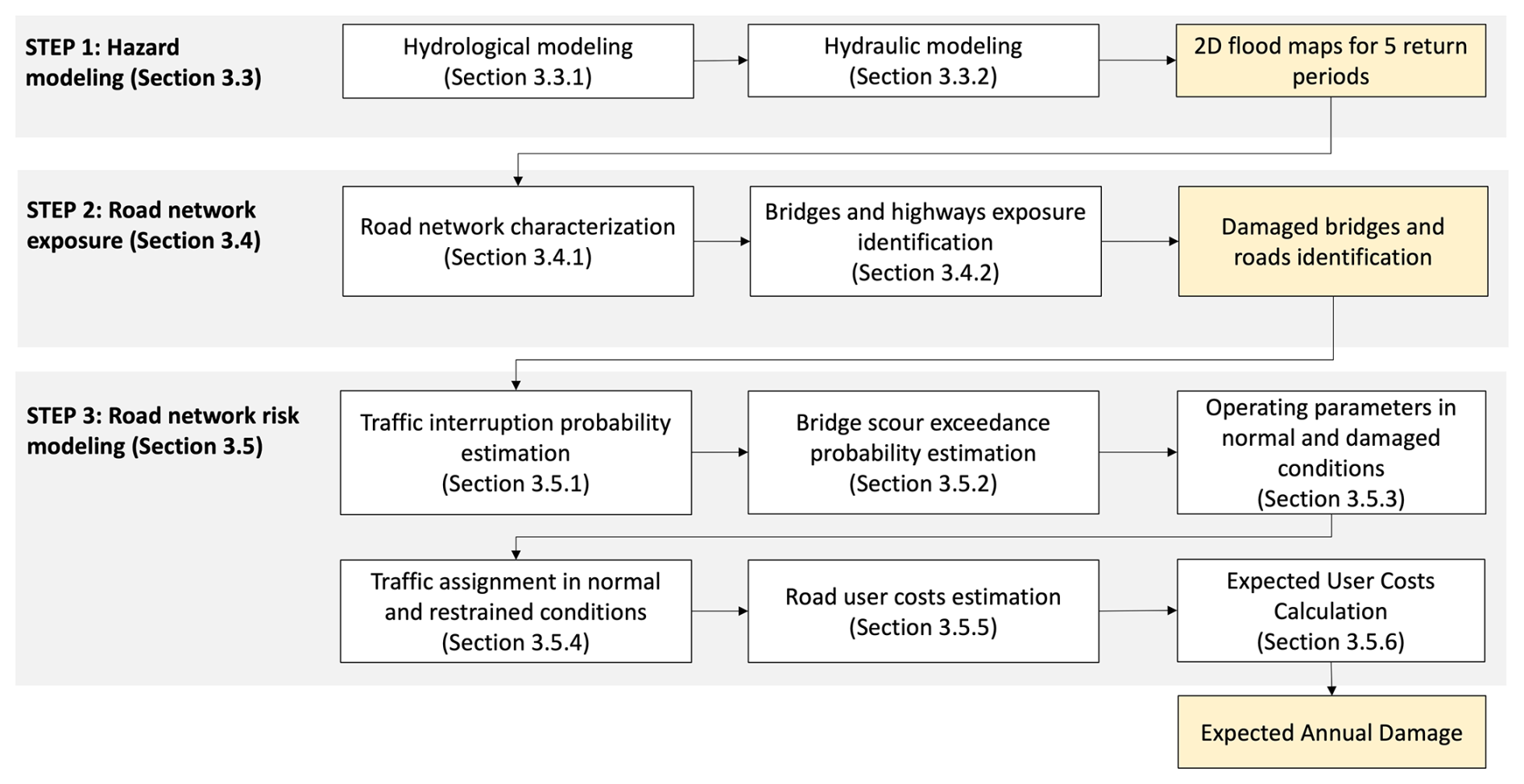
Figure 1 Procedure for calculating road network flooding risk,comprising three steps: (1) hazard modeling (Sect. 3.3), producing 2D flood maps for five return periods; (2) road network exposure analysis (Sect. 3.4), identifying damaged bridges and roads; and (3) road network risk modeling (Sect. 3.5), combining traffic interruption and bridge scour probabilities with traffic assignment and road user cost estimation to obtain the expected annual damage. Yellow boxes indicate the main output of each step; white boxes indicate individual modeling tasks, with the corresponding subsection numbers in parentheses.

The input data for the HMH module were as follows:

• Morphometric data: topography, river network, rainfall-contributing area, main channel length, and average slope

• Hydrological data: maximum rainfall in 24 h for a return period of 10 years and maximum annual discharge.

• Road network data: spatial representation of road links, nodes, and bridges; their physical characteristics, such as cross-section width, pavement type, and capacity; and operational characteristics, such as average speed, traffic volume, and vehicle traffic composition.

3.3 Step 1: Hazard modeling

In the HMH module (step 1), flood maps are obtained as follows: a) estimation of hydrographs at the entrance of each sub-watershed by hydrological modeling and b) spatial representation of flood by 2D hydraulic modeling for each return period. If discharge data are available, flood hydrographs are obtained by tracking floods in the daily maximum discharge registers. If discharge data are unavailable, a hydrograph can be obtained using locally calibrated rainfall-runoff models. The maps indicate the flood surfaces, maximum heights, and maximum flow velocities for various return periods.

3.3.1 Hydrologycal modeling

Hydrological modeling was performed using the Verni and King (1977) rainfall–runoff model, calibrated for Chilean basins with areas between 20 and 10 000 km² and mixed nival–pluvial regimes, which was consistent with the watershed considered in the case study. The lower Aconcagua river Basin was divided into eight subwatersheds, each with a control point at its outlet, for which the watershed area, channel length, slope, elevation difference, time of concentration, and 24 h design rainfall were collected. For each PC, peak discharges were estimated for return periods of 2, 10, 25, 50, and 100 years, respectively. Synthetic unit hydrographs were derived and adjusted such that the time to peak matched the concentration time of each sub-watershed. Finally, by convolving these unit hydrographs with the design rainfall, one design flood hydrograph was generated for each return period at each control point. These hydrographs were subsequently used as inflows for the hydraulic simulations.

3.3.2 Hydraulic modeling

Hydraulic modeling was performed with HEC-RAS 2D using the ALOS PALSAR digital elevation model (12.5 m × 12.5 m resolution) as terrain input, ensuring consistency with the topographic data used in the hydrological analysis. The Manning's roughness coefficients of each sub-watershed were assigned using land use/land cover information collected from satellite images. For each return period, the design hydrographs obtained at the PCs were imposed as the input flow boundary conditions. The HEC-RAS model simulated flood propagation over the Aconcagua River floodplain and its tributaries, and the outputs were processed to generate maps of flood extent, representing the maximum water depths. Finally, the maximum flood depth at each grid cell and return period was extracted for subsequent intersection with the road networks.

3.4 Step 2: Road network exposure modeling

In step 2 (RE), the flood-affected road network was identified by superimposing the flood maps for each return period on the road network map. The flood maps represent the maximum flood depth at each pixel for every return period. For each road segment, the maximum flood depth along the segment was extracted from these maps and used as input to the traffic interruption probability model (Eqs. 5 and 6), and the speed reduction model (Eq. 7), as it represents the most restrictive condition for traffic operability.

3.4.1 road network characterization

Road network characterization involves the following tasks: specification of a node-arc configuration of the road network potentially affected by floods, identification of road type (multilane, two-lane class 1, and two-lane class 2) and road bridges, and specification of operative parameters (average travel speed, capacity, pavement roughness, and vehicle classes in traffic flow). Finally, these attributes are introduced as properties of each arc of the road network. The obtained road network is then prepared to apply the traffic assignment model and estimate road user costs.

3.4.2 Bridge and highway exposure identification

Bridge and highway exposure was obtained by overlapping the road network and flood maps obtained in the hazard modeling. The resulting maps allow the identification of bridges affected by floods and flooded highway segments. Each segment is cut off from the arc, and a new segment is reconfigured. This step is necessary to assign the operating parameters under the damaged conditions.

3.5 Step 3: Road network risk modeling

In Step 3 (RM module), the traffic interruption probability models (Eqs. 5 and 6) are exponential functions calibrated for the Chilean vehicle fleet, estimating the interruption probability for light and heavy vehicles as a function of flood depth, accounting for the variability in wading depth across representative vehicle types (Contreras-Jara et al., 2018). The bridge vulnerability model estimates the exceedance probability of the design scour depth as a function of the water depth (Contreras-Jara et al., 2021). The RM module then identifies the road network characteristics and determines the traffic capacity and operating speed at each network link under normal and restrained operating conditions. Under normal operating conditions, no network links are physically affected by floods. In a restrained operation, one or more network links are partially or fully disabled owing to a flood, forcing traffic to reroute, or speed reduction. Restricted operating conditions in flooded links were assumed if the waterlogging probability exceeded a predetermined value. The circulation speed was calculated using the model proposed by Pregnolato et al. (2017a). Finally, a traffic assignment model is applied under normal and restrained conditions.

3.5.1 Traffic interruption probability estimation

The traffic interruption probability model for flooding, given by Eqs. (5) and (6) for light (P_int-light) and heavy (P_int-heavy) vehicles, respectively, were used to estimate road vulnerability. Contreras-Jara et al. (2018) calibrated Eqs. (5) and (6) for Chilean conditions using reliability principles. The models estimate the probability of traffic interruption in terms of the flood height (h, m).

$$\begin{array}{}\text{(5)}& {\displaystyle }& {\displaystyle }{P}_{\text{int-light}}=\mathrm{1}-e^{-\mathrm{79.829}{h}^{\mathrm{5.223}}}\text{(6)}& {\displaystyle }& {\displaystyle }{P}_{\text{int-heavy}}=\mathrm{1}-e^{-\mathrm{0.137}{h}^{\mathrm{12.917}}}\end{array}$$

3.5.2 Bridge scour exceedance probability estimation

Bridge vulnerability was calculated using the model proposed by Contreras-Jara et al. (2021). This model estimates the scour exceedance probability of one- or two-span bridges exposed to local scouring. The exceedance probability was estimated based on the maximum water depth and the return period.

3.5.3 Operating parameters under normal and restricted traffic conditions

The operating parameters under normal traffic conditions are assigned to each bridge and arcs unaffected by floods. The defect parameters were those described in Sect. 3.4.1. In bridges and road arcs affected by floods detected in Sect. 3.4.2, operative restraints are introduced, from which the more relevant limit probabilities are estimated using Eqs. (5) and (6), and the speed limits in the flooded road arc were estimated using Eq. (7).

For each return period, the probability obtained using Eqs. (5) and (6) set a limit on the water height and determine whether each link operates under normal and restricted conditions. In the flooded links, the limit values of P_int-light and P_int-light is set at 15 %, consistent with the upper calibration limit of the speed reduction model of Pregnolato et al. (2017a, b) for light vehicles at h = 0.3 m. The same threshold is applied to heavy vehicles using Eq. (6), yielding a flood depth limit of h = 1.0 m. The traffic conditions were as follows:

• If h < 0.3 m, light and heavy traffic operate under restricted conditions.

• If 0.3 m < h < 1.0 m, light traffic is interrupted, and rerouting is required. Heavy traffic operates under restricted conditions.

• If h > 1.0 m, light and heavy traffic were interrupted. Re-routing is needed.

Under restricted operating conditions, the traffic speed on roads and bridges is reduced. On flooded road arcs, the speed is calculated using the model calibrated by Pregnolato et al. (2017a, b) (Eq. 7), which estimates the speed limit of light vehicles in the event of flooding (V_lim, km h⁻¹) from the height of the flood on the road (h_R, mm). For larger vehicles, a height limit of 1000 mm was used to estimate V_lim.

$$\begin{array}{}\text{(7)}& V_{\text{lim}}=\left\{\begin{array}{ll}\mathrm{0.0009}{h}_{\mathrm{R}}^{\mathrm{2}}-\mathrm{0.5529}{h}_{\mathrm{R}}+\mathrm{86.9448}& ;h_{\mathrm{R}}\le \mathrm{300}\mathrm{mm}\\ \mathrm{0}& ;h_{\mathrm{R}}>\mathrm{300}\mathrm{mm}\end{array}\right.\end{array}$$

3.5.4 Traffic assignment model

The traffic assignment model (TAM) of Beckmann et al. (1955), extended by Nie et al. (2004), was used. A diagram of this process is shown in Fig. 2. The diagram describes the main features of the traditional traffic assignment model described in Eqs. (8) to (13). The input data were arranged in a travel matrix format. After the road network was characterized (Sects. 3.4.1 and 3.5.3), the optimization model estimated the unit travel time and traffic volume for each arc. Finally, the unit travel time is multiplied by the traffic assigned to each arc and summarized to obtain the total travel time of the network. These values are used as inputs to estimate the expected user cost (EUC) for restrained and normal traffic operations in the network.

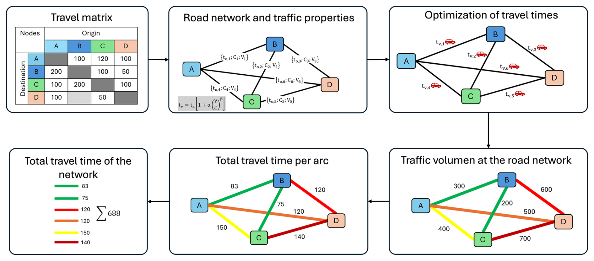
Figure 2 Diagram of the traffic assignment model (TAM). Based on an origin-destination trip matrix and the road network with the properties of its links (top row), the model iteratively optimizes the travel times for each arc (top right; the red cars indicate traffic flow) to obtain, for each arc, the total travel time and the assigned traffic volume (bottom row, from right to left) and, finally, the total travel time for the network. The colours in the “Total Travel Time per Arc” and “Traffic Volume on the Road Network” panels are for illustrative purposes only and represent a qualitative scale ranging from low (green) to high (red) in terms of relative travel time and traffic level, respectively; they do not correspond to the actual values from the case study.

TAM assigns traffic to a road network “G” composed of “N” nodes and “A” links, thereby minimizing the total travel time. The optimization problem is formulated in Eqs. (8) to (13). The optimization problem is typically solved using the Frank–Wolfe algorithm.

$$\begin{array}{}\text{(8)}& min\sum _{a\mathit{ϵ}A}\underset{\mathrm{0}}{\overset{f_a}{\int }}{t}_a\left(x\right)\mathrm{d}x\end{array}$$

In Eq. (8), where “a” represents each link of network “G,” “f_a” is the traffic in link “a,” and “t_a” is the total travel time in link “a,” calculated using Eq. (13). The “a” links of the network “G” are obtained from national road surveys, with which a connected network is prepared. The traffic “f_a” is obtained from national traffic surveys and is generally expressed as average annual daily traffic (AADT). The restrictions on the optimization model are as follows (Bar-Gera, 2002; Nie et al., 2004).

$$\begin{array}{}\text{(9)}& \begin{array}{rl}& \text{Total\hspace{0.17em}\hspace{0.17em}vehicle\hspace{0.17em}\hspace{0.17em}flows\hspace{0.17em} }\text{equal\hspace{0.17em}\hspace{0.17em}to\hspace{0.17em}\hspace{0.17em}the\hspace{0.17em}\hspace{0.17em}demand\hspace{0.17em} }\\ & \text{for\hspace{0.17em}\hspace{0.17em}each\hspace{0.17em}\hspace{0.17em}origin-destination: }\sum _{p\mathit{ϵ}{P}_w}{h}_p=T_w;w\mathit{ϵ}W\end{array}\end{array}$$

$$\begin{array}{}\text{(10)}& \begin{array}{rl}& \text{Traffic\hspace{0.17em}\hspace{0.17em}in\hspace{0.17em}\hspace{0.17em}the\hspace{0.17em}\hspace{0.17em}link\hspace{0.17em}\hspace{0.17em}is\hspace{0.17em}\hspace{0.17em}the\hspace{0.17em} }\text{sum\hspace{0.17em}\hspace{0.17em}of\hspace{0.17em}\hspace{0.17em}the\hspace{0.17em}\hspace{0.17em}flows\hspace{0.17em}\hspace{0.17em}of\hspace{0.17em}\hspace{0.17em}all\hspace{0.17em} }\\ & \text{routes\hspace{0.17em}\hspace{0.17em}that\hspace{0.17em}\hspace{0.17em}use\hspace{0.17em}\hspace{0.17em}the\hspace{0.17em}\hspace{0.17em}link:}{f}_a=\sum _{p\mathit{ϵ}{P}_w}{\mathit{\delta }}_{ap}{h}_p;a\mathit{ϵ}A\end{array}\end{array}$$

$$\begin{array}{}\text{(11)}& \text{No\hspace{0.17em}\hspace{0.17em}traffic\hspace{0.17em}\hspace{0.17em}negativity\hspace{0.17em} }\text{on\hspace{0.17em}\hspace{0.17em}route “}p\text{”: }{h}_p\ge \mathrm{0};p\mathit{ϵ}{P}_w\end{array}$$

$$\begin{array}{}\text{(12)}& \text{No\hspace{0.17em}\hspace{0.17em}negative\hspace{0.17em}\hspace{0.17em}traffic\hspace{0.17em} }\text{in\hspace{0.17em}\hspace{0.17em}link\hspace{0.17em}\hspace{0.17em}“}a\text{”: }{f}_a\ge \mathrm{0};a\mathit{ϵ}A\end{array}$$

$$\begin{array}{}\text{(13)}& t_v=t_a^{\mathrm{0}}\left[\mathrm{1}+\mathit{\alpha }{\left({\displaystyle \frac{f_a}{c_a}}\right)}^{\mathit{\beta }}\right]\end{array}$$

In Eqs. (9) to (12), where “w” is a travels origin-destination (O-D) pair; “W” is the set of all O-D pairs in the “G” network; “P” represents all possible routes in the road network. It can be obtained from an O-D survey or zoning of the study area, and traffic data from national surveys estimate the traffic (h_p) at each link “a” that connects each zone. “P_w” is the set of available routes connecting the O-D pair “w” which are obtained from the network “G”; “T_w” is the traffic in the O-D pair “w” that are obtained from the network “G”. “h_p” is the traffic in route “p”; and “δ_ap” is a dummy coefficient (δ_ap = 1 if the link “a” belongs to the route “p”; otherwise, δ_ap = 0). In Eq. (13), “t_a” is the travel time in the link “a” (h); “$t_a^{\mathrm{0}}$” is the travel time (h) of link “a” in free-flow condition, which is obtained by dividing the length of each link by the average travel speed or by the design speed. “c_a” is the capacity of link “a” ($\mathrm{pcu}{\mathrm{h}}^{-\mathrm{1}}{\mathrm{lane}}^{-\mathrm{1}}$), which can be obtained from TRB (2016). Generally, the capacity of two-lane rural roads ranges between 1400 and 1800 ($\mathrm{pcu}{\mathrm{h}}^{-\mathrm{1}}{\mathrm{lane}}^{-\mathrm{1}}$), and multilane rural roads vary between 2000 and 2200 $\mathrm{pcu}{\mathrm{h}}^{-\mathrm{1}}{\mathrm{lane}}^{-\mathrm{1}}$. These variations depend on whether the terrain is flat, rolling, or mountainous. The parameters α and β were obtained from the TRB (2010 and 2016) (α = 1.5 and β = 5 for multilane and Class 1 roads; α = 1.2 and β = 5 for Class 2 roads).

3.5.5 Road user costs

The speed, traffic volume, and travel time of each road network link are then determined. These outputs are used to estimate the total road user cost (RUC), which is the sum of the travel time cost (TTC) and fuel consumption cost (FCC), as expressed in Eq. (14). The road user cost (RUC) is the sum of these costs per link and vehicle type. The total costs for the network under normal and retrained conditions are the sum of the road user costs of each link and vehicle type. The cost difference between normal and restrained conditions results in operational losses after flooding.

$$\begin{array}{}\text{(14)}& \text{RUC}=\text{FCC}+\text{TTC}=\left[\sum _{a=\mathrm{1}}^A\sum _{v=\mathrm{1}}^{V_a}{d}_a{\text{FC}}_v{f}_v+\sum _{v=\mathrm{1}}^V{t}_v{s}_v\right]\end{array}$$

In Eq. (14), where “V” is the traffic assigned; “V_a” is all vehicles assigned in the link “a”; “d_a” is the length of the link “a” (km); “FC_v” is the fuel consumption of vehicle “v” (mL km⁻¹); “f_v” corresponds to the unit cost of fuel for vehicle “v” (USD L⁻¹); “t_v” corresponds to the travel time of vehicle “v” (h) obtained from the TAM; “s_v” is the unit cost of the time for vehicle “v” (USD h⁻¹). The unit fuel consumptions of light vehicles (FC_lv, $\mathrm{mL}{\mathrm{pcu}}^{-\mathrm{1}}{\mathrm{km}}^{-\mathrm{1}}$) and heavy vehicles (FC_hv, $\mathrm{mL}{\mathrm{pcu}}^{-\mathrm{1}}{\mathrm{km}}^{-\mathrm{1}}$) were calculated using Eqs. (15) and (16), depending on the pavement roughness (IRI, m km⁻¹) and operating speed (OS, km h⁻¹). FC_v is then obtained by converting FC_lv and FC_hv from mL to L.

$$\begin{array}{}\text{(15)}& {\displaystyle }& {\displaystyle }{\text{FC}}_{\text{lv}}=(\mathrm{1255.7}-\mathrm{1.7735}\cdot \text{IRI})\cdot {\text{OS}}^{-(\mathrm{0.543}-\mathrm{0.0009}\cdot \text{IRI})}\text{(16)}& {\displaystyle }& {\displaystyle }{\text{FC}}_{\text{hv}}=(\mathrm{8308.2}-\mathrm{10.085}\cdot \text{IRI})\cdot {\text{OS}}^{-(\mathrm{0.3048}-\mathrm{0.0004}\cdot \text{IRI})}\end{array}$$

3.5.6 Expected user cost

The expected user cost (EUC) is used as a proxy for flood risk in road networks. The EUC (in USD yr⁻¹) is computed by integrating the user road cost (RUC) across return periods using the trapezoidal rule, as expressed in Eq. (17), where T₁–T₅ are the return periods of 100, 50, 25, 10, and 5 years, respectively, and S₁–S₅ are the road user costs (RUC) for each return period, estimated using Eq. (14).

$$\begin{array}{}\text{(17)}& \text{EUC}={\displaystyle \frac{S_{\mathrm{1}}}{T_{\mathrm{1}}}}+\sum _{i=\mathrm{1}}^{n-\mathrm{1}}\left({\displaystyle \frac{\mathrm{1}}{T_{i+\mathrm{1}}}}-{\displaystyle \frac{\mathrm{1}}{T_i}}\right)\cdot {\displaystyle \frac{S_i+S_{i+\mathrm{1}}}{\mathrm{2}}}\end{array}$$

4 Case study and application: Road Network of Aconcagua Basin

4.1 Study area

The study area is known as lower Aconcagua River Basin (LAB) (Fig. 3). The basin originates 4 km downstream of San Felipe City at the confluence of the Aconcagua and Putaendo Rivers. It belongs to the larger watershed of the Aconcagua River, in the central zone of Chile, and extends between 32°44^′ S, 70°46^′ W and 32°55^′ S, 71°31^′ W.

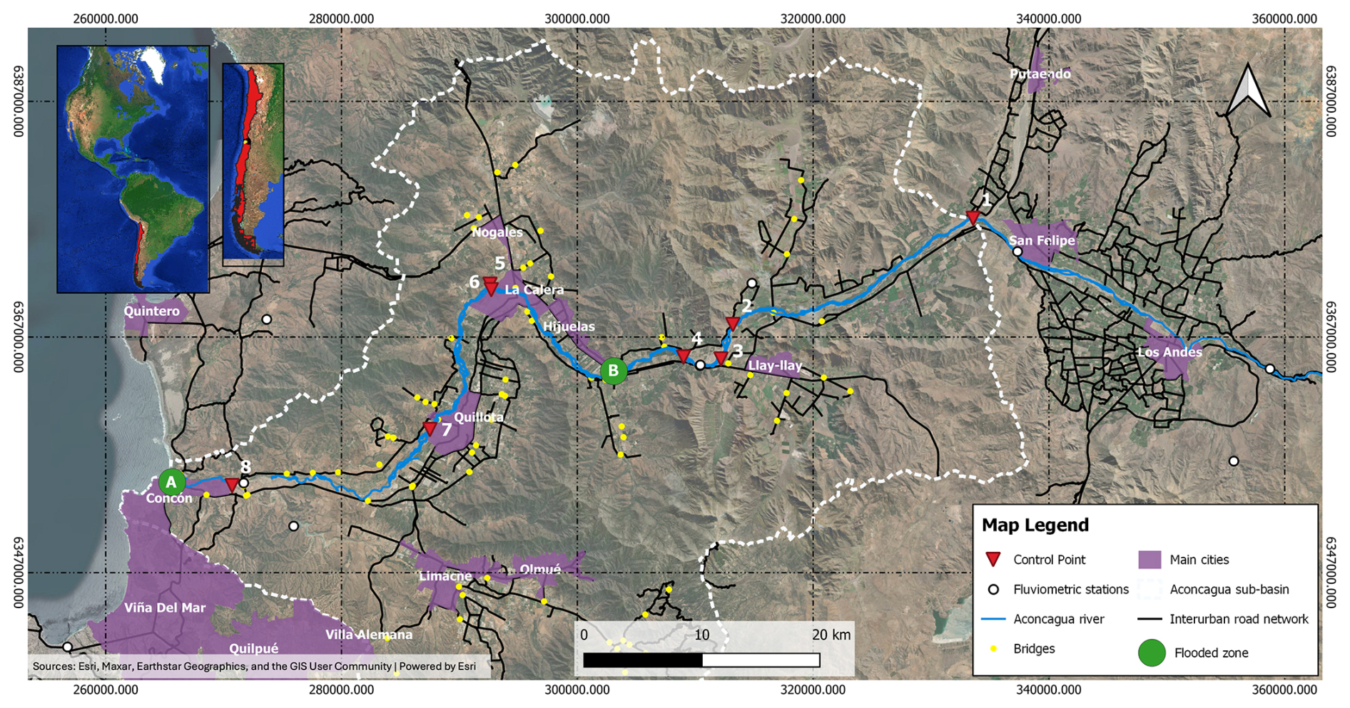
Figure 3 Location and general characteristics of the study area in the lower Aconcagua River sub-basin, central Chile. Insets (top left) show the regional location within South America and Chile. Numbered red triangles (1–8) indicate the control points (PC1–PC8) used for hydrological modeling (Tables 2–4); yellow dots indicate bridges; white circles indicate fluviometric stations; the blue line indicates the Aconcagua River; black lines indicate the interurban road network; purple polygons indicate the main cities; the dashed white line delimits the Aconcagua sub-basin. Green circles labeled A and B indicate the two zones shown in detail in Figs. 4 and 5, respectively. Base map: Esri World Imagery (Sources: Esri, Maxar, Earthstar Geographics, and the GIS User Community | Powered by Esri). Coordinate system: WGS 84/UTM zone 19S.

The main watercourse of the LAB is the Aconcagua River, which is 152 km long and flows from the east to the west. The watershed has an area of 2625 km² and an average flat slope between 160 and 200 m km⁻¹. It has a mixed pluvial-nival regime, a monthly average discharge between 20 and 50 m³ s⁻¹, and a maximum rainfall in 24 h between 80 and 110 mm in a return period of 10 years (MOP, 2004, 2019a). The road network in the LAB is mainly linear and spatially located on the margins of the floodplains in the watershed. The road network comprises two multilane roads connecting the cities of Los Andes, La Calera, Quillota, Concon, and Viña del Mar, and a complementary network composed of two-way, two-lane rural roads. Two percent of the watershed land use is urban and 13 % of the surface is used for forestry and agricultural activities. In addition, 35 % of the land was wooded, 32 % was grassland, 4 % was water bodies, and the remaining 14 % was un-vegetated. Industrial activity is present in the cities mentioned, and agricultural use occurs in rural areas adjacent to the watercourses (MOP, 2004).

The road network under study is in the ancient floodplain of the Aconcagua River, with the main road network on both banks of the river. Road networks near towns and cities have subnetworks that provide accessibility between towns, farms, and main roads. These subnetworks have a geometric design standard that is lower than that of the main route of the network.

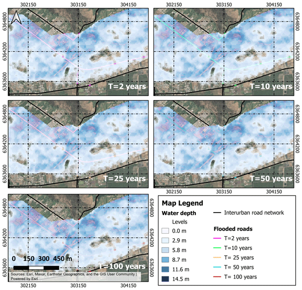
Figure 4 Zone A (see Fig. 3): flooded roads and bridges, their lengths, and flood heights for each return period (T = 2, 10, 25, 50, and 100 years). Shaded blue tones indicate water depth in meters (see legend); coloured lines indicate flooded road segments for each return period. Base map: Esri World Imagery (Sources: Esri, Maxar, Earthstar Geographics, and the GIS User Community | Powered by Esri). Coordinate system: WGS 84/UTM zone 19S.

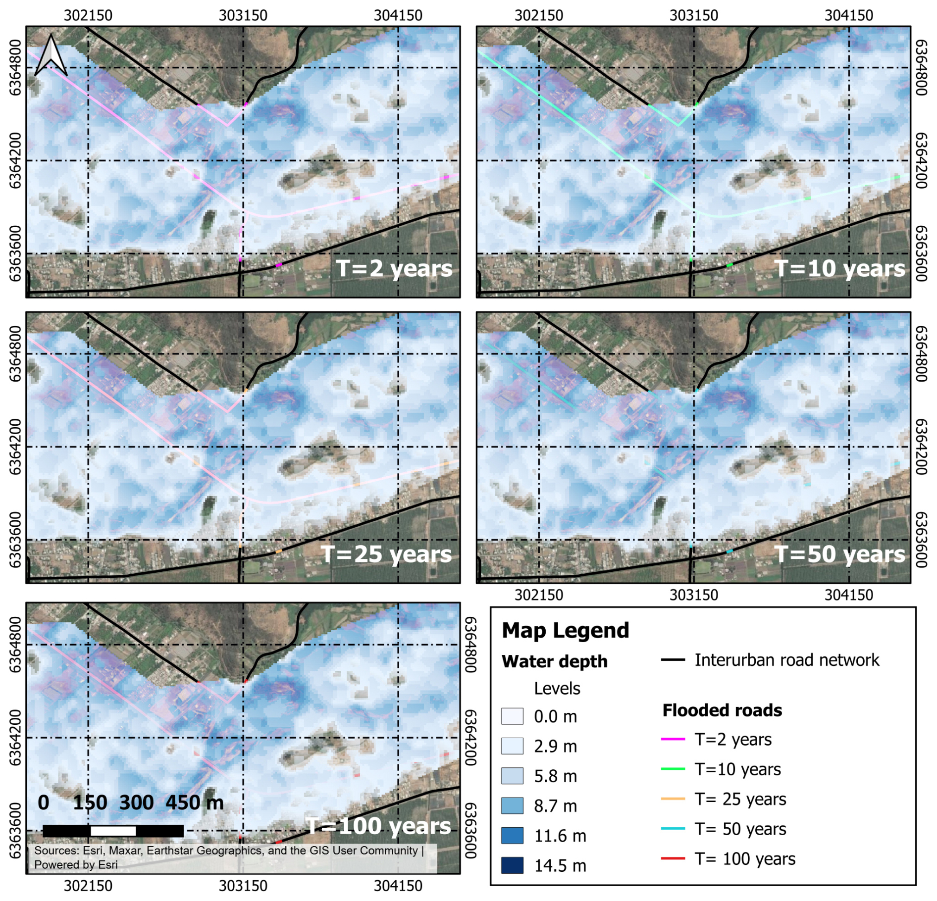
Figure 5 Zone B (see Fig. 3): Flooded roads and bridges, their lengths, and flood heights for each return period (T = 2, 10, 25, 50, and 100 years). Shaded blue tones indicate water depth in meters (see legend); coloured lines indicate flooded road segments for each return period. Base map: Esri World Imagery (Sources: Esri, Maxar, Earthstar Geographics, and the GIS User Community | Powered by Esri). Coordinate system: WGS 84/UTM zone 19S.

The road network in the study area and its specific characteristics were obtained from the geodatabase of roads of the Chilean Ministry of Public Works (MOP 2020a, b). The roads were classified into three categories according to the average speed and road capacity: multilane, two-way, and two-lane Class 1 roads; and two-way and two-lane Class 2 roads (see Table 6). The principal road network consisted of 307 km of multilane roads and 1516 km of two-way, two-lane Class 1 and Class 2 roads, all of which were paved. On multilane roads, each carriageway cross-section consists of two lanes (3.5 m wide each), a 2.5 m-wide shoulder, and a 6 m wide median. On two-way, two-lane roads, the cross-section consists of one lane per traveled way, a lane width of 3.5 m, and shoulders of 1.5 m.

The road network has 79 bridges, with lengths ranging between 10 and 530 m. Nine bridges cross the main watershed river (Aconcagua River). Of these, 75 % are one-span bridges, and the remaining 25 % are two or more span bridges. The annual average daily traffic (AADT) and its composition were estimated using the traffic database of the Chilean Ministry of Public Works (MOP, 2020c) available online. On multilane roads, the AADT varied between 4670 and 17 670 vehicles per day-year. On Class 1 roads, the AADT varied between 605 and 9449 vehicles per day-year. On Class 2 roads, the AADT varied between 1105 and 8015 vehicles per day-year.

4.2 Flood hazard modeling

4.2.1 Flow modeling by return period

Hydrological modeling was performed using a rainfall-runoff model calibrated for Chile by Verni and King (1977) in watersheds between 20 and 10 000 km², with return periods of less than 100 years and a mixed nival-pluvial regime. In the case study, the watersheds had areas between 1638 and 3860 km², and modeling was performed for return periods of up to 100 years; therefore, the model of Verni and King (1977) is applicable to the situation represented in the case study.

Regarding the input parameters used, the topography was obtained from the ALOS PALSAR digital elevation model developed by the Japanese Aerospace Exploration Agency in its JAXA 2011 mission (ASF DAAC, 2014). The resolution was 12.5 m × 12.5 m. Hydrographic data were obtained from the Chilean Ministry of National Land (MOP, 2017). Geomorphological data of the watershed were obtained from post-process topography, hydrographic information, and the contributing areas. The model of Verni and King (1977) used as input data the maximum rainfall in 24 h for a return period of 10 years ($P_{\mathrm{24}}^{\mathrm{10}}$, mm), watershed area, duration factors, and return period factor to adjust the maximum flow in every watershed without fluviometric data. Parameter $P_{\mathrm{24}}^{\mathrm{10}}$, was obtained from the online Hydrometric System of the General Directorate of Waters of the Ministry of Public Works of Chile (MOP, 2019a). All the data are freely accessible.

Hydrologic modeling was performed using a rainfall-runoff analysis owing to the lack of flow information for the entire Aconcagua Basin. For this purpose, flood routing was performed by dividing the basin into eight sub-basins, each with its own attributes and precipitation data. In addition, eight checkpoints (PC) were set at the end of each sub-watershed, including the main channel of the Aconcagua River (Fig. 3). Each PC had a specific data input depending on the runoff-contributing area (Ap). Table 2 shows the input data of each PCi.

Table 2 Morphometric and hydrological input data used in the rainfall–runoff model (Verni and King, 1977) at each of the eight control points (PC1–PC8, Fig. 3).

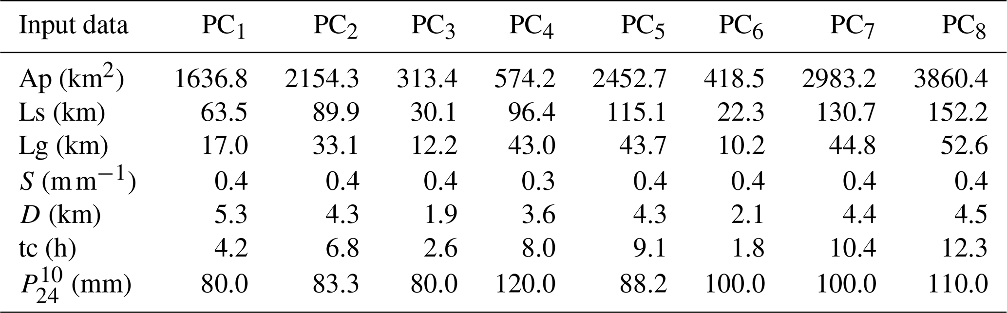
Ap: basin area; Ls: length of the channel upstream of PC_i; Lg: distance between the center of gravity of the basin and the location of the PC_i; S: average slope of each basin obtained from the digital elevation model (DEM) using the QGIS Slope tool (QGIS Development Team, 2021); D: maximum height difference between the highest point of the basin and the PC_i; tc: time of concentration in each virtual sub-basin; $P_{\mathrm{24}}^{\mathrm{10}}$: maximum rainfall in 24 h for a 10-years return period (T).

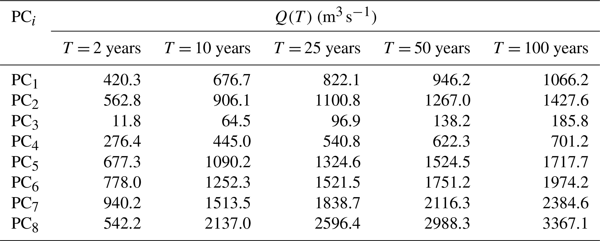
As the first step of the modeling, using the model of Verni and King (1977) as a function of the parameters described in Table 2, the flow rates for return periods of 2, 10, 25, 50, and 100 years were obtained (Table 4). Then, based on the parameters in Table 3, the synthetic unit hydrograph of each sub-basin was obtained and adjusted according to the flow obtained using the Verni and King (1977) model and the time of concentration “tc” of each sub-basin. The criterion used was that the concentration time was equal to the time required to reach the peak value. As a result of hydrologic modeling, five hydrographs for each return period were obtained for the eight sub-basins.

Table 3 Synthetic unit hydrograph parameters derived for each control point (PC1–PC8, Fig. 3), used together with the design rainfall to generate the flood hydrographs for each return period.

t_p: time to peak discharge; t_b: base time; q_p: peak discharge.

Table 4 Peak discharge Q(T) (m³ s⁻¹) estimated at each control point (PC1–PC8, Fig. 3) for return periods T = 2, 10, 25, 50, and 100 years, obtained from the synthetic unit hydrographs in Table 3.

4.2.2 Flood map estimation

HEC-RAS 2D software (USACE, 2016) was used for hydraulic modeling. The same ALOS PALSAR digital elevation model (12.5 m × 12.5 m resolution, ASF DAAC, 2014) used for hydrological modelling was used as the terrain input for the HEC-RAS 2D hydraulic simulations. Manning's roughness coefficients, assigned to each sub-watershed based on land use/land cover classification derived from satellite imagery following Chow et al. (1988), were used as the surface roughness input. Flood hydrographs estimated from hydrological modeling for each return period were used as the boundary conditions for the HEC-RAS 2D model. The same return period was simulated for the entire lower Aconcagua River Basin. The floodable area was identified and assigned roughness and slope, and the input and output hydrographs were obtained from the DEM used for hydrologic modeling. These data were used to estimate the flood surface, flood height, and flow depth of the bridges, roads, and riverbanks in the area. The hydraulic model output represented the maximum flood depth for each return period in the eight sub-watersheds. Figures 5 and 6 show the flood surface and maximum flood depth in zones A and B of Fig. 3.

Figure 6 Traffic assignment model calibration results under normal operating conditions: modeled traffic ($\mathrm{pcu}{\mathrm{h}}^{-\mathrm{1}}{\mathrm{lane}}^{-\mathrm{1}}$) versus traffic from the National Traffic Survey ($\mathrm{pcu}{\mathrm{h}}^{-\mathrm{1}}{\mathrm{lane}}^{-\mathrm{1}}$). Each point represents one road segment (link) of the network (R² = 0.98). The solid black line indicates the 1:1 correspondence between modeled and surveyed values. Labeled outlier points correspond to Hijuelas (1) and Limache (2, 3).

The significant scarcity of comprehensive real-time precipitation data across the entire Aconcagua Basin, with reliable records limited to only two stations situated in the headwaters, precludes the direct use of actual rainfall for the comprehensive hydraulic model calibration and validation. Consequently, the Verni and King (1977) hydrological model was employed to estimate the discharge. Full model calibration or validation using actual distributed rainfall was not feasible under these data constraints; rather, the estimated flows were verified against limited fluviometric station data.

Data from two available fluviometric stations (San Felipe and Llayllay) were used to verify discharge over a 25-year return period. However, insufficient discharge and correspondingly low water height records at these stations precluded the validation of simulated flows. Consequently, verification must be conducted at specific locations using sufficient data. Therefore, PC1 can only be verified for a 25-year return period. The maximum measured discharge at this control point was 800 m³ s⁻¹, which was associated with T = 25 years (Alvarez-Garreton et al., 2018). The discharge modeled for this return period was 822 m³ s⁻¹, which was 3 % greater than the measured value.

Similarly, the specific discharge reported by Alvarez-Garreton et al. (2018) was 0.153 ${\mathrm{m}}^{\mathrm{3}}{\mathrm{s}}^{-\mathrm{1}}{\mathrm{km}}^{-\mathrm{2}}$, and the model was 0.147 ${\mathrm{m}}^{\mathrm{3}}{\mathrm{s}}^{-\mathrm{1}}{\mathrm{km}}^{-\mathrm{2}}$, which is 4 % less than the former. Therefore, the modeled flows were assumed to be valid for 25 years. In addition, water height data were compared with data from an existing fluviometric station in the lower Aconcagua River basin. The data from the fluviometric station showed water heights between 4.4 and 4.8 m for a maximum discharge of 800 m³ s⁻¹. The modeled water height resulted in values between 4.7 and 5.2 m for a return period of 25 years. The maximum difference was 8 %.

4.3 Road network exposure to floods

The road network was overlaid on the flood maps obtained from the hydrological–hydraulic simulation to identify flood-affected road infrastructure. The flooded road segments, lengths, and maximum flood depths were identified for each return period. Road surface elevations were obtained from the ALOS PALSAR DEM (12.5 m × 12.5 m, ASF DAAC, 2014) extracted at the centerline of each road segment. Given the vertical margin of error of the DEM, more precise road surface elevations cannot be derived from this data source. Bridges with a probability of scour design exceedance greater than zero were also identified. Table 5 summarizes the results. Figures 4 and 5 highlight the flood surface and water depth in zones A and B in Fig. 3.

Table 5 Flood-affected roads and bridges for each return period (T = 2 to 100 years), by road category (Multilane, Two-way Two-lane Class 1, Two-way Two-lane Class 2) and bridge type (1-span, +1-span).

H_av: average water depth in flooded roads (m); L: total length of flooded roads (m)

4.4 Road network risk modeling

4.4.1 Modeling parameters

Road network risk modeling considers the reduction of expected costs for network users under normal and restricted conditions. Table 6 lists the parameters under normal and restricted conditions for each road type and vehicle class. The design speed and highway capacities under normal operation were obtained from MOP (2019b). For bridges, the operating speed was set to 20 km h⁻¹ when the scour design exceedance probability was 0.3 and 0.6. Total traffic disruption was assumed for exceedance probabilities higher than 0.6 with an operating speed of 0 km h⁻¹. We assumed that the capacity of the flooded roads remained constant at different flood heights and that only the speed changed, according to the model proposed by Pregnolato et al. (2017a). Above these values, the capacity is zero owing to traffic interruptions. For bridges, it was assumed that scour probabilities between 0.3 and 0.6 are in such a state of damage that traffic and structural capacity are reduced (Hackl et al., 2018). Under these conditions, the reduction in bridge capacity was estimated to be 20 %, assuming normal conditions for vehicles (Bocchini and Frangopol, 2011). For exceedance probabilities greater than 0.6, traffic interruption was assumed; therefore, the traffic and structural capacities of the bridge were considered zero.

Table 6 Operating parameters of the road networks under normal and flood-restricted conditions, by road category, road asset (roads and bridges), and vehicle class, used as input to the traffic assignment model.

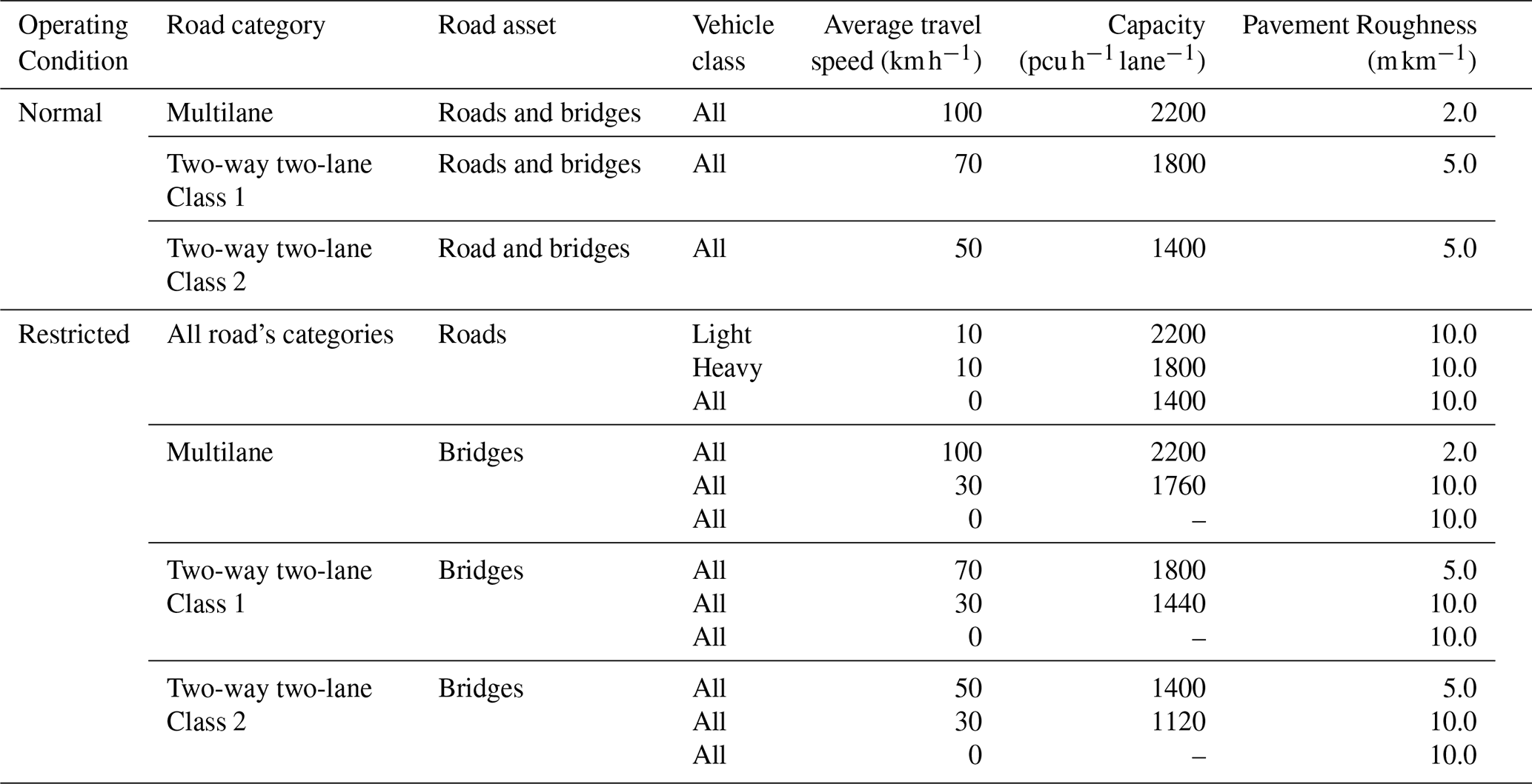
4.4.2 Traffic assignment to the road network

The traffic assignment model applied in this study was solved using the Kumar (2019) code, aiming to optimize traffic flow across the network and minimize travel time under both normal and flood-affected conditions. This model leverages national traffic data and road network characteristics to simulate how floods reroute traffic and increase the user costs. The traffic assignment model uses road and traffic data obtained from national road and traffic surveys conducted by the Chilean Ministry of Public Works (MOP): the National Road Network geodatabase (MOP, 2020b; https://mapasvialidad.mop.gob.cl/visores-2/, last access: 11 May 2026), its dimensions and characteristics (MOP, 2020a), and the National Traffic Survey 2019 (MOP, 2020c; https://vialidad.mop.gob.cl/plan-nacional-de-censo-vial/, last access: 11 May 2026). All datasets were freely accessible online. It also uses a travel time function that considers the capacity and traffic of different road types. The model was applied successively for each return period to obtain the cost-return period pairs with which the loss model was prepared.

The network was built with 154 links and 129 nodes using GIS. Six modeling networks were considered: one representing the normal operating conditions and one for each of the five return periods. The operational physical attributes for the normal and restricted operating conditions were assigned to each link according to the following rules:

• Physical attributes under normal conditions, road class, and length of each link.

• Physical attributes under restricted conditions, road class, length of each link, flooded segment, flood height, and the link to which the flooded segment belongs.

• Operating attributes under normal and restricted conditions are shown in Table 6.

Traffic data were obtained from the National Traffic Survey, issued for two years each, and are freely available on the Chilean Ministry of Public Works website (MOP, 2020c). These data were used to estimate the origin destination matrix. After applying TAM, the modeled traffic was compared with the existing flows in the road network. Figure 6 shows the correlation between the modeled and actual traffic data. Traffic was expressed as passenger car units per hour per lane ($\mathrm{pcu}{\mathrm{h}}^{-\mathrm{1}}{\mathrm{lane}}^{-\mathrm{1}}$). The outlier data points represent traffic in the cities of Hijuelas (Point 1) and Limache (Points 2 and 3).

4.4.3 Road user costs

The road user cost (RUC) was estimated using Eq. (14) for each return period. The fuel consumption models in Eqs. (15) and (16) were obtained from the HDM-4 model calibration developed by the Chilean Ministry of Public Works (MOP, 2018). A travel time unit cost of USD 18.6 h⁻¹ per light vehicle and USD 64.0 h⁻¹ per heavy vehicle was used. The unit fuel costs are USD 0.5 and USD 0.6 L⁻¹ for light and heavy vehicles, respectively (MDS, 2020). These values correspond to the social prices published by the Chilean Ministry of Social Development for 2020 and were converted from Chilean pesos at the average exchange rate of that year (CLP 800 per USD). All monetary values in this study are therefore expressed in 2020 US dollars, and no inflation adjustment was applied.

4.4.4 Road network risk obtained

The total EUC obtained was USD 5.7 × 10⁶ year⁻¹. This cost represents the additional travel time and fuel consumption costs owing to vehicle rerouting in the network caused by flooded road segments, bridge closures, or heavy traffic restrictions on damaged or weakened bridges in the road network under consideration. The accuracy of the estimated EUC increased when additional floods with different return periods were added to Eq. (17). Figure 7 shows the expected losses in terms of the road user costs of the network and each return period.

Figure 7 Expected annual losses in terms of road user cost (RUC, USD thousands) for the road network, plotted against (a) the annual exceedance frequency (T, years⁻¹) and (b) the return period T (years). Points indicate the RUC estimated for each of the five return periods analyzed (R=2, 10, 25, 50, 100 years); the area under the curve in (a) correspond to the expected user cost (EUC) obtained via trapezoidal integration (Eq. 15).

Figure 7 shows the estimated benefits of flood abatement on the road network. According to Penning-Rowsell and Green (2000), if abatement measures are set for a return period of 100 years, then the expected annual benefits are approximately equal to the EUC obtained in this case study. However, to estimate the net benefit, it is necessary to assess higher return periods, estimate the abatement costs at each bridge and road segment affected by floods, and apply the TAM to recalculate the road user and fuel consumption costs for new rerouting schemes. In addition, it shows the avoided costs when implementing risk abatement measures on roads and bridges to ensure the operational continuity of the road network after flooding. The results also allow for the assessment of the benefits of keeping roads open after a flood to permit evacuation and pay attention to people affected by floods.

5 Results discussion

This study extends current practice in three respects. First, risk is expressed as an expected user cost rather than as a reconstruction cost, so that the additional travel time and fuel consumption borne by users are integrated over the event probabilities within the same expected-damage framework used for physical damage. Second, hazard, exposure, vulnerability, and traffic assignment are linked in a single workflow, in which the flood depth for each return-period condition the disruption and scour probabilities of road segments and bridges, and these, in turn, condition the traffic assignment. Third, the procedure relies on open-access data and open-source models, which makes it applicable in basins with limited hydrological monitoring. It thus complements studies that express the consequences of flood-induced road disruption as a loss of accessibility rather than as a cost (Coles et al., 2017; Arrighi et al., 2019; Papilloud et al., 2024).

The flow rates estimated by the Verni and King (1977) model were compared with the available data. This verification indicated that the flows estimated with this model, compared with those available from the PC1 fluviometric station (the only spot check located at the head of the lower Aconcagua River basin), overestimated the 25-year return period by 3 %. This discrepancy subsequently affected the hydraulic modeling results, resulting in an 8 % increase in the estimated flood extent and maximum water height compared with the locally reported values. Such variations may stem from multiple factors, including hydrological model calibration, input topographic data quality, and roughness coefficients. Nonetheless, the values obtained were acceptable for regional-scale simulation.

For the range of analyzed return periods, the following patterns were identified: (a) between two to four sections of flooded multilane roads, with a total affected length of 1.8 to 3.2 km and water heights between 0.5 and 2.2 m; (b) five to ten flooded sections of Class 1 roads with a total affected length between 960 and 3512 m, and flood heights between 1.2 and 2.3 m; and (c) up to two flooded sections of Class 2 roads with a total affected length between 439 and 960 m and flood heights up to 3.7 m. In addition, between one and three bridges with two or more spans affected by flooding were identified, mainly belonging to the multilane and Class 1 two-way two-lane roads.

The vulnerability estimation of roads and bridges was conducted using models calibrated for Chile, considering the characteristics of the local vehicle fleet and the climatic conditions. Therefore, the results for the probabilities of disruption and scour exceedance were suitable for this case study. However, it is crucial to acknowledge that these results are conditioned by the quality of the input data, particularly the digital elevation model and flood map used for each return period.

The traffic assignment model assumes a constant road capacity and static interruption states for each flood scenario based on the maximum flood depth for each return period. The temporal variability of flood depth during an event, which could result in variable capacity and transient interruption states, was not considered in this study.

The traffic modeling results were validated using data from the Chilean Ministry of Public Works. The traffic model calibrated for normal operating conditions demonstrated a solid statistical fit with a coefficient of determination of R² = 0.98, underscoring its accuracy and representativeness. However, this calibration was not performed under restrained traffic conditions after floods, because of unreliable traffic data. Calibration under these conditions requires counting traffic in extensive road networks before and immediately after floods, which is very difficult to achieve. In addition, it should be noted that the 15 % interruption threshold for P_int-light and P_int-heavy, based on the calibration range reported by Pregnolato et al. (2017a, b), is considered a fixed value in this study. In practice, this threshold is uncertain and could be represented as a distribution of damage states, rather than a single criterion, calibrated using field measurements, studies, or other empirical data. The analysis of this sensitivity is left as a line of research for future studies.

EUC estimation implies the combination of datasets, models, and procedures from different origins, which, when combined, introduces errors that propagate throughout the process and affect the results of the study. This study did not include a sensitivity assessment or error identification. However, this type of analysis can be performed using procedures such as those used by Allen et al. (2022), who assessed the sensitivity of the seismic risk assessment of road networks and identified the effect of different error sources on the EUC results.

EUC estimation relies on the following data inputs: digital elevation models, traffic and road network data, and hydrological data (such as discharge and water height). Among these, the resolution of the DEM is a determinant of the accuracy of flood extent and water level modeling. The resolution of the DEM can directly impact vulnerability quantification, as a coarser grid (e.g., 12.5 m × 12.5 m) may identify more potentially affected road assets owing to less detailed terrain and channel bathymetry, leading to potentially overestimated flood extents and depths. Although such a DEM is suitable for preliminary analyses to pinpoint potential flood hotspots, transitioning to a higher resolution (e.g., 5 m × 5 m or 1 m × 1 m) is crucial for a more accurate assessment of vulnerability and, consequently, more reliable indirect cost estimations. This finer resolution allows for detailed site-specific studies in identified high-risk zones, enabling a more precise analysis of the impacts, especially considering that infrastructure dimensions, such as road lane widths (typically 3.5 m), are better represented, leading to a more accurate risk profile for specific assets. Discharge and water height data are required to calibrate hydrological and hydraulic models. However, these data are not always available in terms of their quantity or quality. This situation arises in the studied basin, where only two stations in the basin headwaters provided sufficient data for analysis. Consequently, Verni and King's (1977) hydrological model calibrated for Chile was used. The model relies on the maximum precipitation isohyets to estimate flows. However, the results obtained by the model were generally more significant than the data available for validation, which may have propagated errors in downstream flow modeling and, consequently, in flood map simulation.

Regarding hydraulic simulation, it is important to note that the flood map representation assumes a time-less scenario, graphically displaying only the maximum depth obtained from the simulation for each return period. Consequently, the model does not consider the temporal dynamics of flooded areas, including their appearance and disappearance over time, which can significantly affect traffic assignments. Furthermore, the deterministic approach adopted in this study does not account for the uncertainty inherent in the hydraulic modeling and simulation process, including uncertainty in the model inputs, calibration metrics, and flood predictions. Probabilistic flood mapping approaches are recognized as a more robust alternative and a valuable direction for future work according to the proposal of Huang and Merwade (2022, 2024) and Gomez et al. (2024)

Other aspects affecting the results were road and bridge vulnerability and the RUC models. Both models depend on local conditions and infrastructure design, which are based on design standards. Therefore, models from literature are not recommended for this type of analysis. This study used previously calibrated models for Chilean conditions to represent vulnerability and RUC.

Future research should focus on enhancing hydraulic modeling by moving beyond the current reliance on static flood maps, which typically represent only the maximum inundation depths. For example, this study assumed a constant flood duration of two hours. However, the development of dynamic models that can simulate the complete temporal evolution of flood events, including their initiation, duration, and recession, is crucial. Such advancements, even when utilizing a DEM of the same resolution, would enable a more qualified representation, differentiating between areas experiencing brief transient inundation and those subjected to prolonged periods of significant water depth. This dynamic perspective reveals that the vulnerability of road assets is not static but varies over the duration of an event. Consequently, traffic reassignment also becomes a dynamic process as network accessibility changes over time. This, in turn, would require corresponding improvements in traffic modeling to accurately capture and respond to this temporal variability in flood impacts and network conditions, thereby providing a more realistic understanding of overall system resilience.

Furthermore, given that Expected User Cost (EUC) estimation integrates outputs from sequential hydrological, hydraulic, vulnerability, and traffic models, understanding the propagation of uncertainties is vital. Errors introduced at any stage can cascade through the modeling chain and affect the results of the study. A critical area for investigation is the implementation of a comprehensive sensitivity analysis, such as the approach employed by Allen et al. (2022), which covers the entire workflow. Such an analysis would identify the most influential parameters and data sources contributing to uncertainty and quantify how these errors propagate and impact the final EUC estimation, thereby strengthening the reliability of the risk assessment.

6 Conclusions

This study presents a method for estimating the expected user cost of a network affected by floods in terms of the return period and the costs involved in traffic rerouting owing to total or partial traffic interruption of roads and bridges. This method was applied to a case study of the road network of the lower Aconcagua River basin in central Chile. Flood hydrographs were generated using rainfall-runoff models calibrated for Chile. An open-source digital elevation model and traffic assignment model were also used. This study contributes to the existing literature by providing a comprehensive model that integrates hydrological-hydraulic analysis with road and bridge vulnerability assessments to estimate the EUC, a perspective that has not been thoroughly explored in previous studies.

The effects of floods on bridges and roads were analyzed, mainly because the road network is located on flat ground without cut slopes and embankments of significant heights in the area's natural terrain. However, analyzing the hydrometeorological hazards on road networks located on undulating or mountainous terrain requires including the effects of slopes, sliding slopes, debris flows, and more detailed digital elevation models than the one used. Furthermore, vulnerability and traffic interruption models must be considered natural hazards in steep or undulating terrains.

The traffic assignment was made considering that the origin-destination matrix was not modified by the effect of the modeled flood owing to its duration. An important aspect of future research is the analysis of the effect of flood road interruptions on non-travel decisions and their costs, as well as the modeling of traffic reassignment from flood onset to lowering water levels to normal values. Such research requires a dynamic traffic assignment model and in-depth analysis of how the travel matrix evolves during floods.

The expected user cost was aggregated on the network because the traffic assignment model does not identify the proportion of traffic that reroutes from one link to another in the road network or to which link it reroutes. Resolving this situation requires a traffic allocation model using an agent-based microsimulation model that enables the identification of individual behavior patterns in the network and the calculation of the risk level per link.

Network redundancy refers to the existence of more than two links connecting two nodes or origin-destination pairs. Redundancy exists if the links are similar in length, platform materials, traffic capacity, and bridges without load restrictions, and satisfy topological conditions based on centrality measures, such as betweenness or closeness. If these conditions are satisfied, two or more links provide redundancy to the road network. In contrast, a road network is non-redundant if the links are significantly different. Under this framework, the lack of redundancy reduces the possibility of traffic rerouting when a flood partially or totally interrupts a link, thereby increasing the travel time in the road network and risk. A detailed analysis of this effect enables decision makers to identify the investments needed in specific road network links to increase redundancy. However, this aspect of road networks was not examined in this study, which offers a research opportunity to improve the flood risk of road networks in the future.

The proposed method integrates the existing procedures to estimate hazards, traffic assignments, and road user costs. This method can be applied directly to other watersheds by considering local parameters. The traffic assignment algorithm depends only on road network properties, traffic data, and origin-destination matrices that can be estimated locally. The road-user cost parameters were obtained from the literature. Only models that estimate traffic interruption and scour exceedance probability must be locally developed and calibrated for each bridge. Therefore, considering local conditions, this procedure can be easily applied to other study areas in the future. The transferable elements are therefore the workflow and the definition of risk as an expected user cost, not the numerical results, which are specific to the Aconcagua Bajo network, its vehicle fleet and its cost parameters. The main weakness of hydrological-hydraulic issues is data availability, which depends on the availability and number of stations for measuring discharge and height over a significant period. Similarly, the availability of detailed land-use information in the watershed is required to estimate the concentration time comprehensively. Regarding traffic, the main challenge is dealing with changes in origin-destination travel, travel not carried out, and the differentiated effect on cargo and passenger travel.

This study did not examine the effect of the lack of redundancy on risk valuation, considering the road network as input data. However, we expect to assess the impact of increasing or reducing alternative routes on risk in future studies. Another relevant challenge is the establishment of error propagation throughout the procedure. This novel research field requires the development of more reliable risk estimations by identifying sources of uncertainty and their propagation.