A Global Ensemble Forecast System (GEFS)-based synthetic event set of U.S. tornado outbreaks

Severe convective storms (SCS) are important drivers of global insured losses, and tornado outbreaks – when many tornadoes occur within a short time span – cause extreme and localized loss of life and property. Tornado outbreak risk estimates from observations, either storm reports or reanalysis environments, are limited by meteorological conditions that have occurred in the historical period. A standard approach of addressing this inadequacy is to construct synthetic event sets that consist of unrealized but plausible events that better represent the full range of possible outcomes. In this study, we constructed and evaluated a synthetic event set of U.S. tornado outbreaks using Global Ensemble Forecast System (GEFS) environments and a tornado outbreak index. With over 800 000 daily maps of environments, over 200 000 synthetic events are generated. In a seamless framework, the synthetic event set includes “daughter events”, constructed from short-lead forecasts and resemble historical events, as well as independent physically plausible events, constructed from longer-lead forecasts. With the GEFS synthetic event set, we estimated that the 1-in-100-year and 1-in-1000-year U.S. tornado outbreak event has 150–250 and 275–400 (F/EF1+) tornadoes per day, respectively. The GEFS synthetic event set also shows robust shifts related to ENSO – higher outbreak activity during La Niña conditions – and trends – increased outbreak activity during 2010–2019 compared to 2000–2009 – consistent with reports. We also developed a subsampling procedure to estimate locally specific tornado outbreak risk, which we illustrate by generating return level curves for grid cells that cover Dallas, Nashville, and Chicago.

1 Introduction

Severe convective storms (SCS) are thunderstorms that produce damaging winds, hail, and/or tornadoes, and they have major socioeconomic implications. In 2023 alone, U.S. insured losses from SCS reached a record USD 58 billion, and 60 % of global catastrophe losses in the first half of 2024 were from SCS (Aon, 2024). In fact, insured losses from SCS have matched or exceeded those from hurricanes over recent decades (Gallagher Re, 2024). Tornado outbreaks – when many tornadoes occur within a short time span – cause some of the most extreme impacts in regards to localized loss of life and property. Therefore, assessments of tornado outbreak risk are of value to society.

Observation-based estimates of tornado and tornado outbreak risk have a number of limitations. The observational record of U.S. tornadoes consists of human-based reports from NOAA Storm Prediction Center (SPC), which began collecting these reports in the 1950s. Between 1979 and 2021, the U.S. on average has approximately 500 tornadoes per year rated 1+ on Fujita/Enhanced Fujita (F/EF) scale, which rates tornado intensity from 0 to 5 based on its damage (Fujita, 1971). About 320 of those 500 tornadoes per year are associated with tornado outbreaks (depending on definition of outbreak), which occurs on ∼30 d of the year. The spatial extent of tornadoes is small: The average path length of a tornado ranges from 4–5 km for F1 to 44–55 km for F4/5, and the average width of a tornado ranges from 64 m for F1 to 460–555 m for F4/5 (though reports reflect mean width until 1994 and maximum width after 1994; Brooks, 2004). EF1 tornadoes occur almost 30 times more frequently than EF4/5. The relatively small footprint of tornadoes means that many locations have never reported a tornado despite presence of environmental/physical conditions conducive for activity. In other words, just because a location has never reported a tornado does not mean the tornado risk at that location is zero; rather, the SPC report record is too short to account for the “randomness” of tornado occurrence. Consequently, the record is likely too short to accurately estimate the characteristics of the most extreme tornado outbreak events, both on a U.S.-scale and at a particular location. Another limitation is that the SPC reports contain non-physical artifacts due to evolving technologies (e.g., Doppler radar), reporting practices (e.g., differences from one forecast office to another, change from Fujita to Enhanced Fujita scale; WSEC, 2006), and population density (Verbout et al., 2006; Edwards et al., 2021). In general, these limitations of tornado reports mean it is difficult to assess tornado outbreak risk with only reports.

Synthetic event sets are the common strategy in catastrophe modeling, climate risk assessment, and insurance and reinsurance for overcoming the limitation of observational data in estimating the risk from rare, impactful natural hazards. The idea is that synthetic events greatly increase the sample size and event diversity in a computationally inexpensive manner while remaining consistent with the observed statistics and/or meteorology, thereby filling spatial gaps and better sampling extremes. Essentially, strategies for constructing synthetic event sets must balance the need that events be physically realistic with the constraint that many events should be generated. For instance, in the case of tropical cyclone (TC) risk, high-resolution physics-based modeling remains prohibitively expensive and simplified models must be used. Consequently, some studies have generated North Atlantic TC genesis and/or tracks with purely statistical stochastic models (Hall and Jewson, 2007; Bloemendaal et al., 2020). Others have incorporated some physics through hybrid dynamical-statistical methods. Emanuel et al. (2006) used simplified physics to simulate TC tracks and intensity. Lee et al. (2018) used physics-informed inputs from reanalysis and climate models to construct a statistical model for TC genesis, track, and intensification. The synthetic event approach has also been used for tsunamis (Davies, 2019), wildfires (Guillaume et al., 2019), flooding (Quinn et al., 2019; Wing et al., 2020), and windstorms (Welker et al., 2021).

For thunderstorms, especially those that produce tornadoes or hail, computational costs are even higher because of the resolution needed to simulate its processes. Additionally, sample sizes need to be larger to account for their small spatial extent. Synthetic event set approaches for tornado risk have also been purely statistical (Daneshvaran and Morden, 2007; Strader et al., 2016; Fan and Pang, 2019) or have used meteorological environments to simulate tornadogenesis favorability (Hatzis et al., 2020). In this ingredient approach, tornado activity/favorability is related to local environmental conditions, typically as some combination of atmospheric instability and vertical wind shear (Brooks et al., 2003; Thompson et al., 2003; Tippett et al., 2012; Cheng et al., 2015, 2016). This strategy is attractive for risk assessment as it fills in “gaps” where environmental conditions were favorable for storms but none were reported. This approach has been useful in weather forecasting contexts, e.g., the Supercell Composite Parameter (SCP) and the Significant Tornado Parameter (STP) are calculated from thermodynamic and dynamic variables to measure the favorability of observed and forecast atmospheric conditions for supercell production (Davies, 1993; Thompson et al., 2003). This approach also has been applied to reanalysis data to explain tornado (outbreak) activity (Brooks et al., 2003; Tippett et al., 2014), understand its climate signals (Malloy and Tippett, 2024; Allen et al., 2015b; Koch et al., 2021), and estimate future projections (Diffenbaugh et al., 2013). In the case of climate signals, using both reports and ingredients, La Niña has been shown to increase tornado (outbreak) activity (Cook and Schaefer, 2008; Allen et al., 2015b; Lepore et al., 2017, 2018; Tippett and Lepore, 2021; Lee et al., 2013, 2016; Malloy and Tippett, 2024). Malloy and Tippett (2024) detected upward trends in 1979–2021 tornado outbreak activity, especially for the winter and spring seasons, consistent with the upward trend in 1979–2015 tornado outbreak activity from Tippett et al. (2016), the upward trend in 1960–2022 tornado outbreak days from Graber et al. (2024), and the upward trend in 1979–2017 STP from Gensini and Brooks (2018), especially for the winter and spring seasons.

However, synthetic event sets generated using reanalysis environments (e.g., Hatzis et al., 2020) are still limited to meteorological conditions that have occurred in the historical record. They fail to capture risk from physically possible but unrealized meteorological conditions, which is especially relevant for rare, high-impact events, such as tornado outbreaks. The relatively short record may not have captured the most extreme (i.e., 1-in-100+ year) tornado events in many locations. To overcome this limitation, some studies of other hazards have supplemented observational data with data from climate model large ensembles or reforecast ensembles, which are large datasets of meteorological conditions produced from running a weather or climate model from slightly different initial conditions (Squire et al., 2021; Thompson et al., 2017; Kelder et al., 2020; Breivik et al., 2014). In this approach, model data is treated in same manner as observational reanalysis data, which allows for direct estimation of extremes without resorting to statistical extrapolation. In the case of reforecast ensembles specifically, the data includes unrealized meteorological conditions that are consistent with climatological frequency and initial conditions; therefore, one can evaluate risk statistics for tornado outbreaks outside the relatively short record of historical events. This approach has been used to assess impacts from windstorms (Osinski et al., 2016; Meucci et al., 2018), extreme rainfall/flood events (Kelder et al., 2020; Thompson et al., 2017; Klehmet et al., 2024; Jain et al., 2020), heatwaves (Coughlan de Perez et al., 2023; Kelder et al., 2022; Kay et al., 2025), and stratospheric polar vortex events (Kolstad et al., 2022). In this work, we use Global Ensemble Forecast System (GEFS) reforecast environments (Hamill et al., 2006) in conjunction with the tornado outbreak index from Malloy and Tippett (2024) to construct a synthetic event set of tornado outbreaks. Considering the 20 years of daily initializations, daily forecasts out 16–35 d, and 5–11 ensemble members, we have over 800 000 daily maps of environments to generate outbreak likelihood maps.

The goal of this work is to construct and validate a GEFS-based synthetic event set of tornado outbreaks, which we use to answer both science and insurance and reinsurance-related questions about tornado outbreaks. We will apply tornado outbreak synthetic event set to construct detailed return level curves, with information about extreme scenarios of hazard risk. The synthetic event set is verified through how it represents the physical world, e.g., we evaluate how the synthetic event set matches observed climatology and variability. We estimate rare events by subsampling the synthetic event set, and we quantify uncertainty in observed and event set tornado outbreak risk estimates. We also evaluate if the GEFS synthetic event set represents climate signals in tornado outbreak activity. Compared to purely statistical approaches, a benefit of using GEFS to construct the synthetic event set is that each event is associated with a date, including a month and year; thus, we can assess ENSO- and trend-related shifts and the robustness in these shifts.

In Sect. 2, we describe the data and methods to construct the synthetic event set. In Sect. 3, we outline results as follows: First, we evaluate tornado outbreak statistics from the GEFS synthetic event set, including comparing short-lead GEFS events and long-lead GEFS events. Then, we explore ENSO-related shifts and trends using the GEFS synthetic event data. Finally, we estimate location-specific tornado outbreak extremes using a subsampling approach with the GEFS synthetic event data. In Sect. 4, we summarize our conclusions, discuss implications of this work, and suggest potential next steps.

2 Data and Methods

2.1 Data

Tornado reports are taken from the NOAA Storm Prediction Center (SPC) Severe Weather Database. We use the 1979–2024 period for report data for most analysis but also compare results to the 2000–2019 period for report data, which matches the GEFS reforecast period. We define a tornado outbreak when six or more tornadoes occur over the contiguous U.S. (CONUS) with no more than 6 h between consecutive tornadoes (Fuhrmann et al., 2014; Malloy and Tippett, 2024, 2025). Tornadoes are labeled as outbreak-level if they meet this criterion. We exclude tornadoes rated 0 on F/EF scale. When labeling outbreak-level tornadoes (hereby called outbreak tornadoes), we do not impose a geographic constraint (Doswell et al., 2006). We construct a dataset of gridded outbreak tornado occurrence at a 6-hourly and 1° × 1° resolution from the SPC report data. The 6-hourly and 1° × 1° resolution matches that of many weather forecast models (and reanalysis datasets), and this resolution is useful for simulating tornado outbreak activity from large-scale meteorological environments. A one in the gridded SPC report dataset means that an outbreak tornado occurred in a given grid cell and 6-hourly period (00:00–06:00, 06:00–12:00, 12:00–18:00, or 18:00–00:00 UTC), and a zero means that an outbreak tornado did not occur. We also consider spatially smoothed occurrence data where we apply a 2D Gaussian kernel smoother with σ=120 km as in Malloy and Tippett (2024) and Malloy and Tippett (2025), similar to “practically perfect hindcasts” (Hitchens et al., 2013; Gensini et al., 2020; Sobash et al., 2020).

Convective precipitation (CP), 0–3 km storm relative helicity (SRH), and mixed-layer convective available potential energy (CAPE) are taken for 2000–2019 from the North American Regional Reanalysis (NARR). NARR provides data at a 3-hourly and 32-km native grid resolution. We resample as a 6-hourly sum for CP and 6-hourly average for SRH and CAPE, and we perform a bilinear interpolation to a 1° × 1° spatial resolution.

Model data of CP, 0–3 km SRH, and mixed-layer CAPE are taken from Global Ensemble Forecast System (GEFS) version 12 reforecasts (Guan et al., 2022). GEFS reforecasts were initialized once per day at 00:00 UTC over the 2000–2019 period. Reforecasts have five ensemble members except for those initialized on Wednesdays, which have an additional six members (eleven total). Reforecasts extend 16 d from their initialization except for those initialized on Wednesdays, which extend 35 d. Reforecasts are originally provided with 3-hourly output and 0.25° × 0.25° spatial resolution for the first 10 d of a forecast, and with 6-hourly output and 0.5 × 0.5° after the first 10 d of a forecast. To keep a consistent resolution, and to match the outbreak tornado occurrence data from reports and NARR, GEFS data is interpolated to 6-hourly output and 1° × 1° spatial resolution.

We use the tornado outbreak index from Malloy and Tippett (2024) to generate synthetic tornado outbreak events. The index has two parts. The first part provides a map of the 6-hourly probability of outbreak tornado occurrence:

$$\begin{array}{}\text{(1)}& \begin{array}{rl}\log \left({\displaystyle \frac{p}{\mathrm{1}-p}}\right)& =-\mathrm{20.2}+\mathrm{0.76}\log \left(\text{CP}\right)\\ & +\mathrm{1.82}\log \left(\text{SRH}\right)+\mathrm{0.51}\log \left(\text{CAPE}\right)\end{array}\end{array}$$

where the left-hand side is the log odds, and p is the probability. The GEFS-based index is computed from the 6-hourly values of CP, SRH, and CAPE from individual GEFS ensemble members. In order to compute the second part of the index, the 6-hourly maps are aggregated to daily maps by taking the maximum value (probability/likelihood) at each grid cell over the convective day (12:00–12:00 UTC). This results in a probability map for each day. The NARR-based index is similarly computed with 6-hourly values of observed/historical CP, SRH, and CAPE and is aggregated to a daily resolution. The NARR-based index represents tornado outbreak occurrence calculated from the 20 years of historical, realized meteorological environments. The index has seasonal cycle deficiencies (Malloy and Tippett, 2024), e.g., probabilities are too high during summer, that are corrected via a post-calibration method. We also applied a post-calibration for the NARR-based index to correct for seasonal cycle deficiencies. Additional information on the processing of the GEFS data, calculation of tornado outbreak index within GEFS, and the post-calibration of the index can be found in Malloy and Tippett (2025). With 20 years of reforecasts initialized daily, each with 5–11 ensemble members and being run out to 16–35 d, GEFS provides 889 514 daily maps (equates to over 2000 years) of outbreak tornado probabilities. Hence, the GEFS-based index represents tornado outbreak occurrence from meteorological environments closely resembling historical, realized meteorological environments as well as unrealized meteorological environments.

The second part of the index calculates the probability distribution of the number of U.S. outbreak tornadoes using one daily probability maps at a time from above via negative binomial regression (Malloy and Tippett, 2024). We recalculated the coefficients for the second part of the index since the NARR-based probability maps are post-calibrated, though results are similar if using coefficients from the second part of the index from Malloy and Tippett (2024). The equation for the expected number of outbreak tornadoes based on the probability map for each day is:

$$\begin{array}{}\text{(2)}& \begin{array}{rl}\mathit{\mu }& =\exp \mathit{\{}-\mathrm{1.14}+\mathrm{2.16}\log \left[\text{sum}\left(P_{\text{CONUS}}\right)\right]\\ & -\mathrm{0.60}\log \left[\text{max}\left(P_{\text{CONUS}}\right)\right]\mathit{\}}\end{array}\end{array}$$

where sum(P_CONUS) is the index map sum and max(P_CONUS) is the index map maximum. In the negative binomial regression, the variance (σ²) is related to the mean (μ) via an overdispersion parameter:

$$\begin{array}{}\text{(3)}& {\mathit{\sigma }}^{\mathrm{2}}=\mathit{\mu }+\mathrm{13.74}\mathit{\mu }\end{array}$$

Equation (3) makes it possible to generate random, or stochastic, realizations of tornado occurrence based on the same daily map of the environments/index. For each daily map of the index, we can generate as many outbreak events as desired, which we call n_realizations, i.e., we can draw n_realizations samples of total U.S. outbreak tornadoes from the probability distribution of part 2 of the index (cf. Eqs. 2 and 3) which are all physically consistent with the large-scale environment. Thus, we further increase the sample size. Then, for each realization, we can populate tornado locations based on map probabilities from the first part of the index (cf. Eq. 1).

Both parts of the GEFS-based index are available on Zenodo. Realizations can be generated as described above using Python scipy library and $scipy.stats.nbinom.rvs$ function, where the dispersion parameter is input as $\frac{\mathrm{1}}{(\mathrm{1}+\mathit{\alpha })}$.

We also demonstrate the use of the tornado outbreak synthetic event set for estimating ENSO variability and trends in tornado outbreak activity. We separate, or subset, activity based on time period, 2000–2009 versus 2010–2019, and El Niño-Southern Oscillation (ENSO) phase. We define ENSO by the Climate Prediction Center (CPC) Oceanic Niño Index (ONI), which is calculated by averaging the SST anomalies over the Niño 3.4 region (5° N–5° S, 120–170° W) and applying a 3-month running mean. We upsample monthly ONI for a daily timescale when labeling events as falling within a particular ENSO phase. A monthly ONI value of ≥0.5 °C would label all the days/events valid during that month as occurring during El Niño, and a monthly ONI value of $\le -\mathrm{0.5}$ °C would label all the days/events valid during that month as occurring during La Niña.

2.2 GEFS Synthetic Event Metrics

We calculate spatially averaged ensemble spread and forecast error – predictability metrics for the ensemble system – to better understand lead-dependent tornado outbreak index behavior in GEFS. The equation for ensemble spread (calculated at each lead time) is:

$$\begin{array}{}\text{(4)}& \mathrm{Spread}\left(\mathrm{lead}\right)=\sqrt{{\displaystyle \frac{\mathrm{1}}{NM}}\sum _{i=\mathrm{1}}^N\sum _{j=\mathrm{1}}^M{\left({\stackrel{\mathrm{‾}}{x}}_i-x_i^{\left(j\right)}\right)}^{\mathrm{2}}}\end{array}$$

where $x_i^{\left(j\right)}$ is ensemble member j index value at grid cell and time i, $\stackrel{\mathrm{‾}}{x_i}$ is the ensemble mean of index at grid cell and time i, M is the ensemble size, and N is the number of grid cell–time samples. We only consider grid cells with an observed climatological tornado frequency of at least 0.01 %, i.e., ignoring locations where tornadoes are very rare.

The equation for forecast error or root mean squared error here (calculated at each lead time) is:

$$\begin{array}{}\text{(5)}& \mathrm{Error}\left(\mathrm{lead}\right)=\sqrt{{\displaystyle \frac{\mathrm{1}}{N}}\sum _{i=\mathrm{1}}^N{\left({\stackrel{\mathrm{‾}}{x}}_i-o_i\right)}^{\mathrm{2}}}\end{array}$$

where o_i is the smoothed report data at grid cell and time i.

We use frequency maps and return level curves to represent tornado outbreak activity from the synthetic event set. Return period is approximated empirically with no assumed underlying distribution. First, we sort and rank the data. The non-exceedance probability, p_e, is $\frac{r}{r-\mathrm{1}}$, where r is the rank. Then, the approximate return period is $\frac{-\mathrm{1}}{\log \left(p_{\mathrm{e}}\right)}$.

2.3 Subsampling Procedure

The number of daily maps is on the order of 10⁵ (and close to 10⁶), and the stochastic component of second part of the index increases the sample size of U.S. tornado total realizations n_realizations-fold (see Eq. 2 and corresponding text), where n_realizations is user-defined and may be ≥10 for risk applications. Therefore, if one were interested in location-dependent outbreak risk, the calculation of this estimate using all the days in the synthetic event set could be computationally expensive and needless. In catastrophe modeling, event sets are often “boiled down”, or condensed to a representative subset that preserves the key statistical risk characteristics of the original event set, to reduce computational cost (Mitchell-Wallace et al., 2017). Here, we provide an illustration or template of a subsampling procedure designed to obtain location-specific (rather than CONUS-wide) daily extreme estimates:

1. We chose a threshold of 6 in expected number (μ) of total U.S. outbreak tornadoes (corresponding to ∼95th percentile). This defined the lower bound of daily maps to keep, i.e. we only kept daily maps where the expected value of total U.S. outbreak tornadoes was 6 or greater. This equates to approximately 40 000 daily maps. We converted the rest of the days that did not meet threshold to zeroes.

2. For the remaining days with at least 6 expected U.S. outbreak tornadoes, we computed 10 realizations of the number of total U.S. outbreak tornadoes, i.e., n_realizations=10, following part 2 of the outbreak index. At this point, the number of daily maps is approximately 400 000.

3. From this subset, we only kept samples with at least 27 tornadoes (equates to ∼85th percentile of this subset), another chosen threshold which boils down the subset to approximately 55 000 daily maps. We converted the rest of the days that did not meet threshold to zeroes. Considering step 1 keeps ∼95th percentile and this step keeps ∼85th percentile, the final subsampled set equates to non-zeros accounting for approximately $\mathrm{100}-\mathrm{100}(\mathrm{1}-\mathrm{0.95})(\mathrm{1}-\mathrm{0.85})$, or $\sim \ge$99.25th percentile days.

4. With the approximately 55 000 daily maps of outbreak likelihood and number of total U.S. outbreak tornadoes, we randomly populated the locations of tornadoes proportional to the outbreak probability. See Sect. 2a and Malloy and Tippett (2024) for more information about how this is done. This is the most computationally expensive part of the procedure and is why subsampling for location-specific information is necessary.

The first user-defined threshold (step 1) manages the number of outbreak likelihood maps, and the second user-defined threshold (step 3) boils the subset down to the most extreme outcomes so that populating locations (step 4) is computationally manageable. The procedure is flexible depending on the user's goals and computational resources. For results that require estimates at the grid point level, such as maps and city-specific return level curves, we use this subsampling procedure to demonstrate its effectiveness to generally estimate outbreak statistics, including extremes (e.g. 99.99th percentile events) in risk.

2.4 Statistical Significance

For observational data, we calculate uncertainty by bootstrapping with replacement for 1000 iterations. For the GEFS data, we calculate uncertainty using the stochastic realizations, i.e., we randomly select an outcome from the distribution generated from part 2 of the tornado outbreak index for 1000 iterations.

3 Results

3.1 GEFS Synthetic Event Set Performance

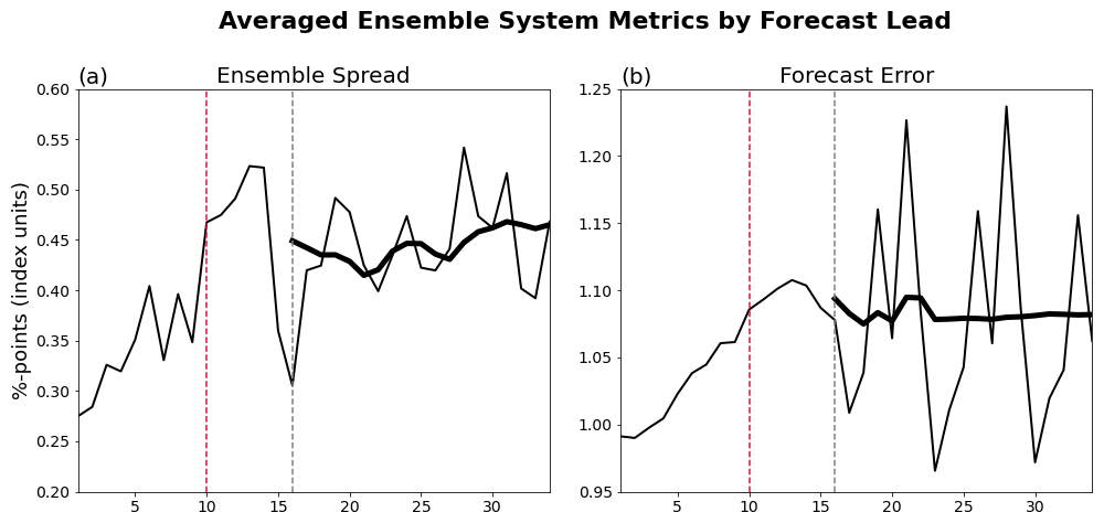
Figure 1 Ensemble system metrics by forecast lead: (a) ensemble spread, or root mean squared error (RMSE) when comparing ensemble mean to individual ensembles, averaged across five ensemble members, and (b) forecast error, or RMSE when comparing ensemble mean to smoothed report data. The dashed crimson lines denote the forecast lead where we separate “short-lead” GEFS and “long-lead” GEFS. The dashed light gray lines denote the 16-d forecast lead; GEFS forecasts with leads of 16 d or more have significantly fewer samples, as only Wednesday initializations extend that far (see text for more details). Thicker solid line shows 7-d (lead time) smoothed spread or error after 16-d leads.

Around lead times of 10 d, predictability of mid-latitude weather diminishes (Zhang et al., 2019; Lorenz, 1982). We label 1–9-d forecasts as “short-lead” and 10+ forecasts as “long-lead” and test whether synthetic event statistics differ between these two sets of GEFS simulations. For instance, we expect that the short-lead forecasts might have relatively reduced ensemble variance in tornado outbreak activity since events look more like the observations and more like each other due to the higher skill and predictability. In contrast, the long-lead forecasts should have higher ensemble variance because they are essentially independent from observations (and each other) and represent draws from climatology. In Fig. 1, we show lead-dependent averaged ensemble system metrics of ensemble spread and forecast error. We observe a divide between 1–9-d forecasts and 10+ d forecasts in terms of these averaged predictability metrics in the tornado outbreak index probabilities. Around the 10-d forecast lead, ensemble spread increases sharply, suggesting ensemble members are more independent from each other after this lead time. Additionally, the forecast error climbs steadily until the 14-d forecast lead. The large variability in forecast error after 16-d forecast leads (denoted by dashed light gray line) is likely due to smaller sample size as only forecasts with Wednesday initializations extend past 16 d (each forecast lead for day 1–15 has ∼3.7 times more data to calculate spread/error compared to each forecast leads for day 16–34).

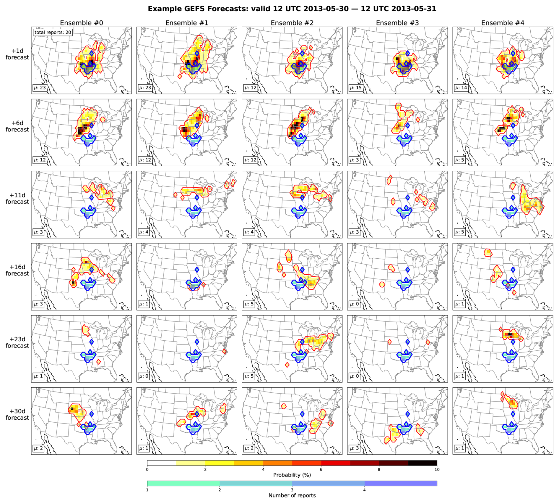
Figure 2 Example of GEFS synthetic events via its forecasts for 2013 12:00 UTC 30 May through 12:00 UTC 31 May, where rows indicate corresponding forecast lead for event, and columns indicate corresponding GEFS ensemble member (only up to 5 members): tornado outbreak index (yellow-red-black shading) versus observed reports (green-blue-purple shading). Expected number (μ) of tornadoes based on outbreak index part 2 given in bottom-left of all panels. Total number of reports for observed event (20 reports) also in top left panel.

An example of the GEFS forecasts and the calculated tornado outbreak index valid for 12:00 UTC on 30 May 2013 through 12:00 UTC on 31 May are shown in Fig. 2. Each row denotes a different initialization time, i.e., increasing lead time, and each column denotes an ensemble member (only up to 5 members here despite 16-, 23-, and 30-d forecasts having 11 ensemble members). The tornado outbreak likelihood (shading) and expected (μ) total number of (outbreak) tornadoes (upper-left of panel) comprise the forecasted tornado outbreak index. The observed reports (blue dots) for that day – 20 in total – are overlaid. For the 1-d forecasts, the tornado outbreak index likelihood well matches the observed reports in regards to location and extent of event. For the 6-d forecasts, the tornado outbreak index likelihood also matches the observed reports in terms of predicting elevated CONUS outbreak risk, though the risk is shifted slightly more north compared to the observed event. In general, these shorter-lead forecasts demonstrate relatively high prediction skill. Moreover, these short-lead forecasts are “daughter events” in the sense that they are other physically possible outcomes to the historical event. Additionally, the ensemble members' tornado outbreak index likelihoods resemble each other in the short-lead forecasts, demonstrating high predictability. In contrast, for the 11-, 16-, 23-, and 30-d forecasts, the region of relatively high tornado outbreak index likelihood looks dissimilar from the observed event, and the events between ensemble members look dissimilar from one another. In other words, the prediction skill and predictability are low. However, tornado outbreak activity still occurs in forecasts beyond day 11. The long-lead GEFS forecasts represent a realistic set of independently drawn events sampled from May climatology, a peak month for tornado activity.

Figure 3 shows the climatological spatial distribution of tornado outbreak activity as represented by the SPC reports, NARR-based tornado outbreak index, and the GEFS-based tornado outbreak index, which we further split into short-lead and long-lead forecasts. Here the locations of tornadoes are populated only based on μ from Eq. (2) rather than also computing realizations for every daily map. The report data climatology (panels a–d) shows the tornado outbreak seasonal cycle, with a peak in climatological activity during March–May (MAM). The report data climatology is spatially noisy due to the relatively short observational record and the sporadic, rare nature of tornadoes. The NARR-based tornado outbreak index climatology (panels e–h) also has a similar spatial distribution and seasonal cycle as in the reports. In general, summer and fall outbreak activity is lower, and spring outbreak activity is higher, in the NARR-based index than in reports. The NARR-based index climatology is also spatially noisy; 20 years of subdaily environments is still insufficient to account for sporadic, rare nature of tornadoes. The GEFS-based tornado outbreak index climatology for the short-lead forecasts (panels i–l) and long-lead forecasts (panels m–p) generally matches that of the report data climatology. However, the long-lead forecasts show greater climatological outbreak activity in winter and spring compared to the short-lead forecasts as well as the reports. This difference is despite the fact that the long-lead and short-lead forecasts have similar climatology in environments conditional on at least 1 % outbreak probability (not shown). The increased ensemble spread of long-lead forecasts (Fig. 1) might explain the increased mean of tornado outbreak index in long-lead versus short-lead forecasts. Larger average values of the index might be expected for long-lead forecasts even though there is little difference in the environment climatologies because the variance is larger for the long-lead forecasts. The reason for this expected increase is that the logistic regression sigmoid function is approximately convex over the range of values here, and a greater variance increases the average of a convex function (convex ordering; Shaked and Shanthikumar, 2007). The GEFS-based index climatology is spatially smoother compared to that of the reports and NARR-based index, suggesting that the increased sample size from the GEFS synthetic events can interpolate tornado outbreak risk. In other words, the GEFS-based index reflects a broader, smoothed representation of tornado outbreak risk, where climatological risk is driven by the frequency of subdaily favorable environments rather than the luck of individual tornado occurrences in a short observational record.

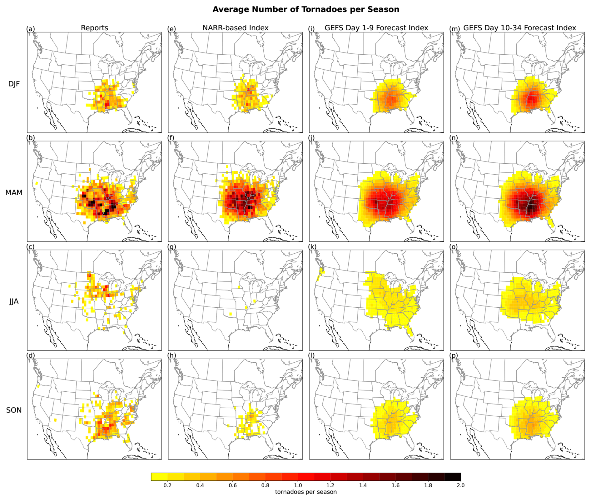
Figure 3 Average expected (μ) number of outbreak tornadoes during (top row) December–February, (second row) March–May, (third row) June–August, and (last row) September–November, calculated from (a–d) reports, (e–h) NARR-based index, (i–l) GEFS short-lead (day 1–9 forecasts) index, and (m–p) GEFS long-lead (day 10–34 forecasts) index.

Next, we present extremes of U.S. tornado activity via return level curves for total number of U.S. outbreak tornadoes per day in Fig. 4 for the (a) full year of data and then separated by (b) DJF, (c) MAM, (d) JJA and (e) SON seasons. Return level curves highlight the right tails of the distribution. We calibrate the frequency of 6-tornado occurrence between the reports and GEFS by scaling the occurrence rate of 6 U.S. outbreak tornadoes a day in GEFS to match the occurrence rate of 6 tornadoes a day in the report data, which corresponds to a shift of the return level curve on a log-log plot. Here the GEFS short-lead full year data for number of outbreak tornadoes are multiplied by 1.44 and the long-lead full year data for number of outbreak tornadoes are multiplied by 1.20. This calibration is also done for each season separately (panels b–e). The observed reports can only resolve a ∼40-year (or 20-year if taking same period as GEFS) return level, whereas the GEFS data can resolve 1000+ year return levels. GEFS synthetic events from the long-lead forecasts estimate the 100-year return level for total daily U.S. outbreak tornadoes to be approximately 200 tornadoes. The GEFS-estimated return level curves closely follow the observed return level curves, though they may overestimate return levels at the most extreme events. Additionally, the long-lead forecasts produce higher estimated return levels compared to the short-lead forecasts, a similar result to Fig. 3. However, overall, the long-lead and short-lead forecasts follow a similar slope or curvature in the return level curves except for the most extreme events, suggesting their variance is similar but the GEFS long-lead event distributions might have a heavier right tail. The heavier right tail in the long-lead forecasts might explain why the climatological index for long-lead forecasts is larger than the short-lead forecasts (cf. Fig. 3). When analyzing return level curves by season, we find that this overestimation of extremes primarily stems from the summer season (Fig. 4d). This is likely related to an issue noted in previous studies, that summer environments might not represent tornado outbreak activity well and overestimate its frequency (Malloy and Tippett, 2024, 2025). The summer return level curves also have sleeper slopes, indicating a heavier right tail of the distribution compared to the reports. The return level curves for the other seasons match the observed return level curves well. For the remainder of the study, we combine the short- and long-lead GEFS forecasts to represent the full GEFS synthetic event set.

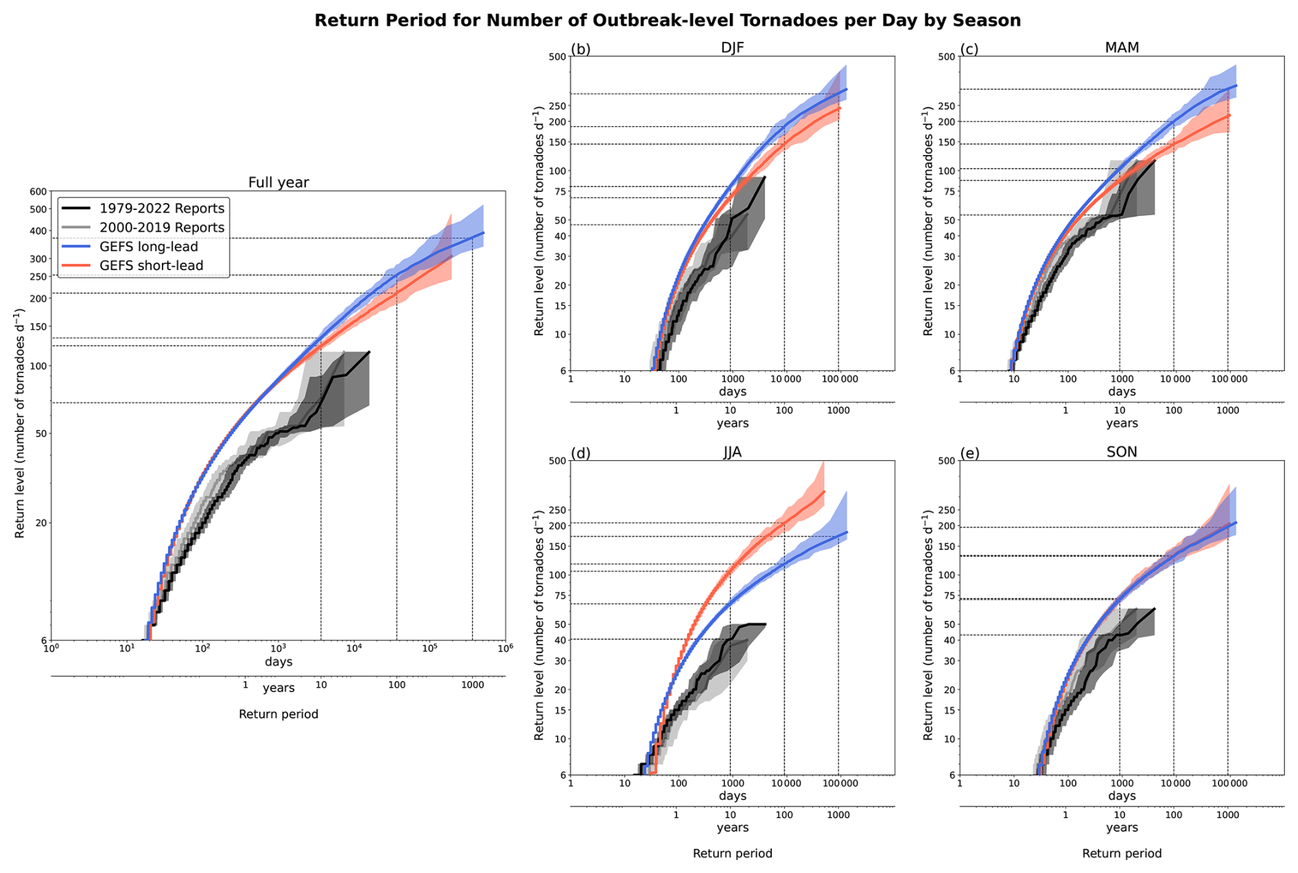
Figure 4 Return level curves for number of outbreak-level tornadoes per day from (black line) 1979–2022 reports, (gray line) 2000–2019 reports, to be consistent with GEFS time period, (blue line) GEFS long-lead forecast, and (orange line) GEFS short-lead forecasts, for (a) full year of data, and for (b) DJF, (c) MAM, (d) JJA, and (e) SON. Shading indicates sampling uncertainty. Dotted lines highlight the 10-, 100-, and 1000-year return period levels.

Figure 5 shows return level curves but for number of U.S. outbreak tornadoes per year. We calibrate the frequency of 100 tornadoes per year between the reports and GEFS by scaling the occurrence rate of 100 U.S. outbreak tornadoes a year in GEFS to match the occurrence rate of 100 tornadoes a year in the report data. The GEFS synthetic events generally capture the variability in annual total of outbreak tornadoes. For instance, both the observed reports and GEFS synthetic events estimate the 10-year return period for annual total U.S. outbreak tornadoes to be approximately 425 tornadoes. The GEFS synthetic event set estimates the 100-year return level to be approximately 575 tornadoes annually.

Figure 5 Return level curves for number of outbreak-level tornadoes per year for (black line) 1979–2022 reports, (gray line) 2000–2019 reports, and (purple line) GEFS synthetic events. Dotted lines highlight the 10-, 100-, and 1000-year return period levels.

3.2 Climate Signals in Tornado Outbreak Activity

Next, we use the GEFS synthetic event set to examine climate-scale influences on tornado outbreak activity. Figure 6 shows the return level for U.S. outbreak tornadoes per day during El Niño and La Niña December–May (DJFMAM) seasons in reports and in the GEFS synthetic event set. In the reports, La Niña (blue curve) is associated with a greater number of outbreak tornadoes per day during DJFMAM, especially for the events with return periods greater than 1 year (Fig. 6a). However, the uncertainty due to sampling overlaps for the El Niño and La Niña curves, especially for the lower return periods. The ENSO-related shift is seen in the GEFS synthetic event set (Fig. 6b) until events with return periods of greater than 10 years. According to the GEFS synthetic event set, the typical winter–spring extreme during La Niña is ∼55 outbreak tornadoes per day, and the winter–spring extreme during El Niño is ∼45 outbreak tornadoes per day. Another way to describe the shift is that a return level of 20 outbreak tornadoes per day during winter-spring occurs every 30 d on average during La Niña and every 50 d on average during El Niño. Interestingly, La Niña and El Niño return level curves (and their uncertainty bars) overlap for the most extreme (right tail) events. The GEFS synthetic events suggest that the extreme events can still occur during El Niño. The reports shows the opposite behavior, that the largest differences between El Niño and La Niña occur for the most extreme events; perhaps the observed record is not long enough to have sufficient number of ENSO events to resolve details in the ENSO-related shifts in outbreak statistics.

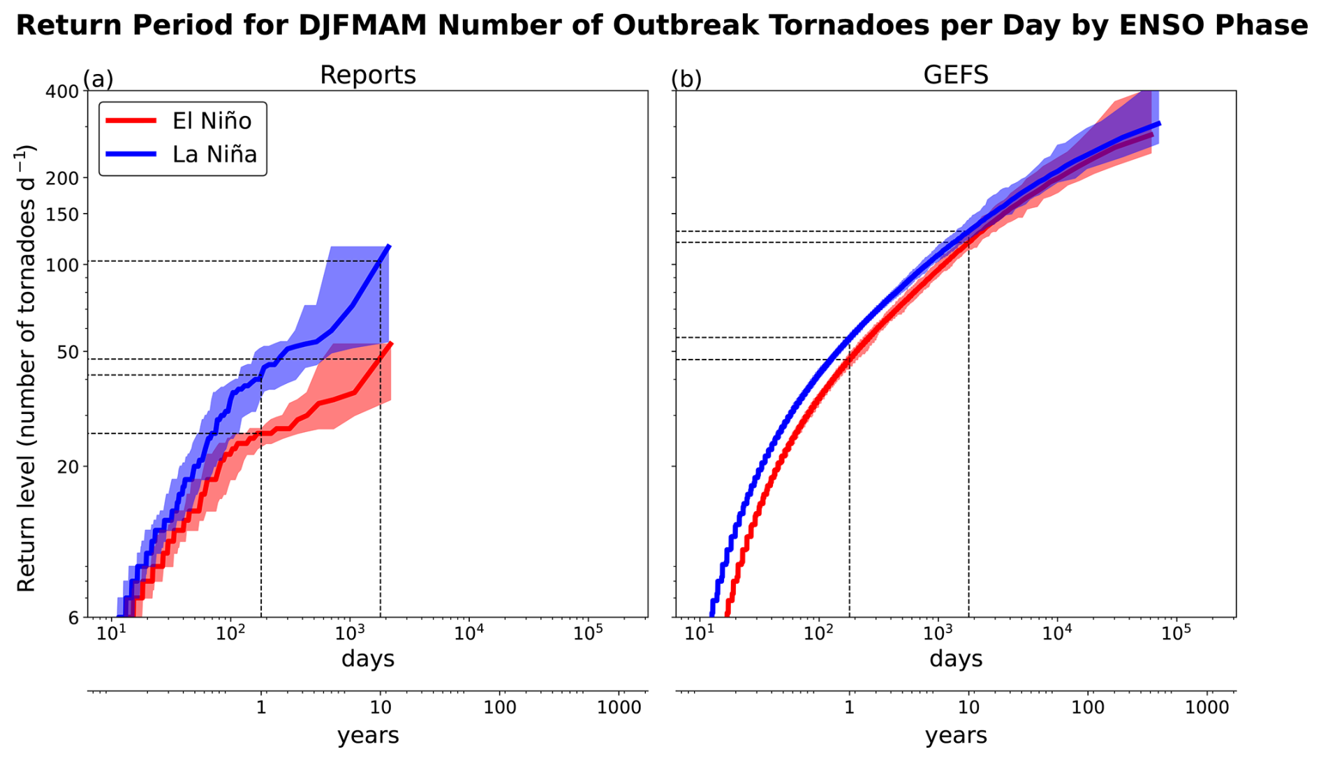
Figure 6 Return level curves for number of outbreak tornadoes per day during December–May (DJFMAM) season during (red line) El Niño days and (blue line) La Niña days, for (a) reports and (b) GEFS synthetic events. Dotted lines highlight the 1- and 10-year return period levels and their differences between El Niño and La Niña.

Figure 7 shows the return period for U.S. outbreak tornadoes per DJFMAM season between earlier (2000–2009) and later (2010–2019) periods in reports versus GEFS synthetic event set. In the reports, the 2010–2019 is associated with a greater number of outbreak tornadoes per DJFMAM season (Fig. 7a), though with considerable overlap between the two periods' sampling uncertainties. The ten years of data for each period is not enough to determine robustness in tornado frequency shifts. In the GEFS synthetic event set, the shift in DJFMAM seasonal totals between the two periods is distinct, i.e., the later period is associated with more outbreak tornadoes per DJFMAM season (Fig. 7b), indicating an increased ability to detect trends. The 1-in-10-year return period in winter–spring seasonal totals in 2010–2019 have almost 100 more outbreak tornadoes compared to 2000–2009. Furthermore, a return level of 300 outbreak tornadoes per winter–spring occurs every ∼5.5 years on average in 2000–2009 period and every ∼2.5 years on average during 2010–2019 period.

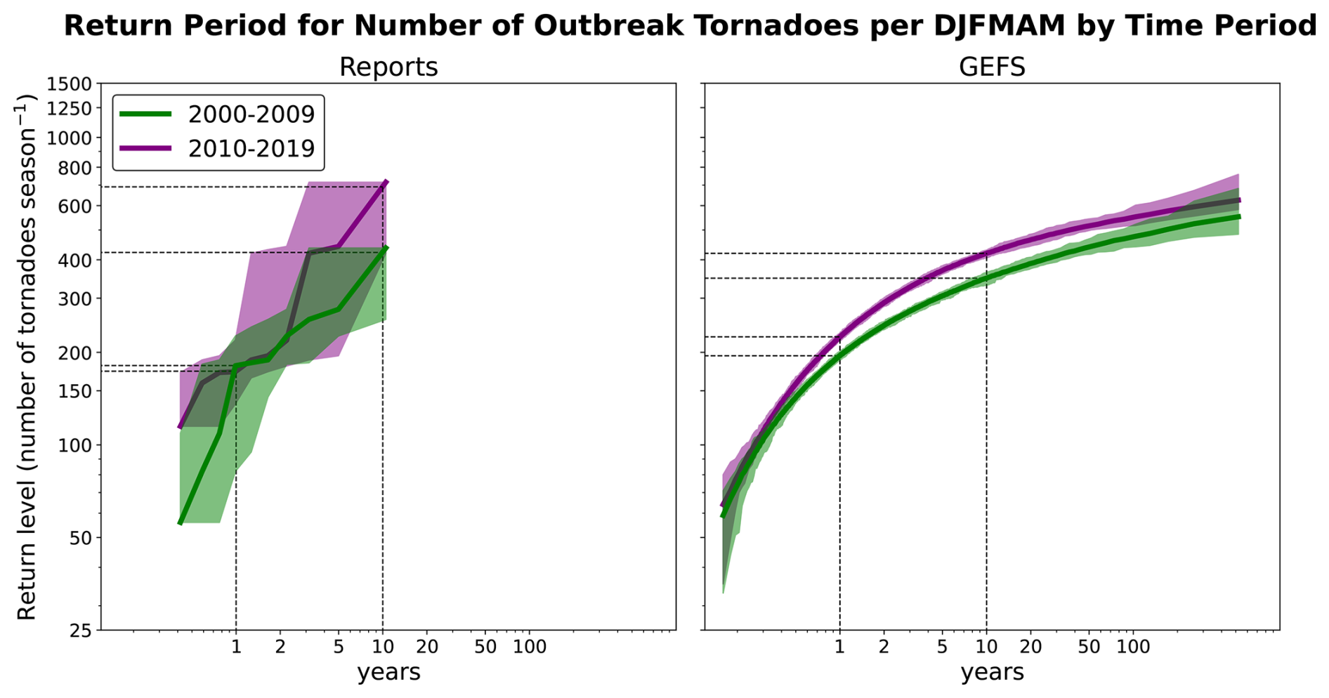
Figure 7 Return level curves for number of outbreak tornadoes per DJFMAM season during (green line) 2000–2009 period and (purple line) 2010–2019 period, for (a) reports and (b) GEFS synthetic events. Dotted lines highlight the 1- and 10-year return period levels and their differences between 2000–2009 and 2010–2019 periods.

3.3 Localized Risk Information for Tornado Outbreak Extremes

The relatively short observational record makes it especially challenging to resolve the risk of tornado outbreaks at specific locations and cities. In Fig. 8, we demonstrate how the GEFS synthetic event set can be used to estimate outbreak statistics, including information about extremes, at individual grid points. In Fig. 8a, b, we compare the 99.99th percentile in outbreak tornadoes per day at every grid point using (a) reports vs. (b) GEFS synthetic event set. The 99.99th percentile is the 1-in-10 000 d event, or approximately equivalent to the 1-in-27 year event. We use the 1979–2021 report data for this estimate due to having 43 years of data versus only 20 years for 2000–2019 period. For the reports, the map of this estimate in this extreme is spatially noisy and difficult to discern. The GEFS synthetic event set better interpolates the estimate in this extreme, showing that the regions with the greatest 99.99th percentile events are over Tennessee River Valley at 4 tornadoes per day at each grid point. Figure 8c shows the factor by which the base rate of GEFS synthetic event set is scaled to match the base rate of the reports. Base rate refers to the frequency of at least 1 outbreak tornado occurring. In general, Texas, the western Plains, and coastal North Carolina and Virginia have underestimated base rates with our subsampling procedure and event numbers need to be multiplied by 3–6. In addition, parts of Appalachia have overestimated base rates and event numbers need to be multiplied by 0.25–0.5.

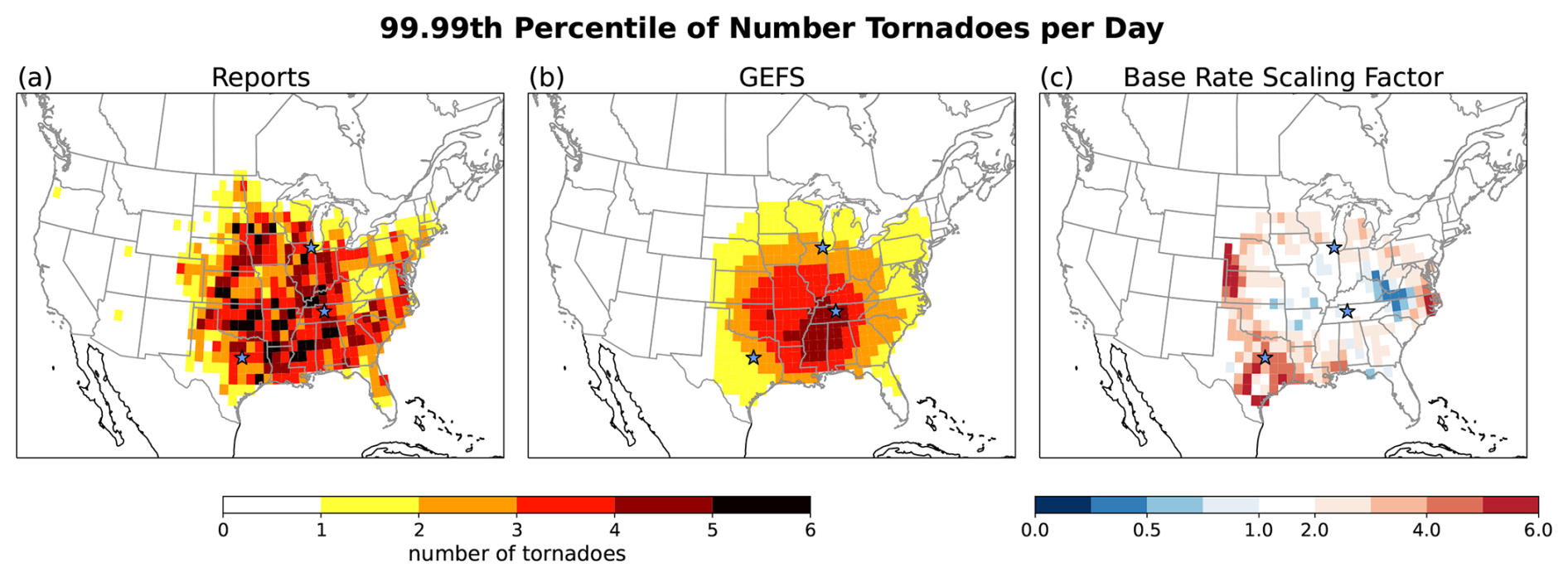
Figure 8 99.99th percentile in outbreak tornadoes per day based on (a) reports and (b) GEFS synthetic event set, with (c) the scaling factor for the base rate (1 outbreak tornado per day) of GEFS synthetic event set fit to reports base rate. Star markers indicate the cities of interest for Fig. 9.

In Fig. 9, we show the return level curves for outbreak tornadoes per day for three major cities: (a) Dallas, (b) Nashville, and (c) Chicago. As demonstrated here, because of our subsampling procedure, the most extreme events (right tail of distribution) are resolved better and extend further into the extremes. As shown in Fig. 8c and described above, we scale the occurrence rate of 1 outbreak tornado a day so that the frequency of 1 outbreak tornado a day from the subsampled synthetic event set is similar to the frequency of 1 outbreak tornado a day from the reports. After scaling of the base rate, the GEFS synthetic event set falls within the uncertainty range of the reports and realistically resolves the extreme (e.g., 100- and 1000-year return levels) days for Dallas, Nashville, and Chicago. This scaling also corrects for the values from the map in Fig. 8b, which shows the 99.99th percentile or 1-in-27 year event, for Dallas, Nashville, and Chicago area to be about 6, 6, and 4 tornadoes per day, respectively. The 1-in-100 year event for Dallas, Nashville, and Chicago area to be about 8, 8, and 6 tornadoes per day, respectively. The 1-in-1000 year event for Dallas, Nashville, and Chicago area is about 15, 17, and 12 tornadoes per day, respectively.

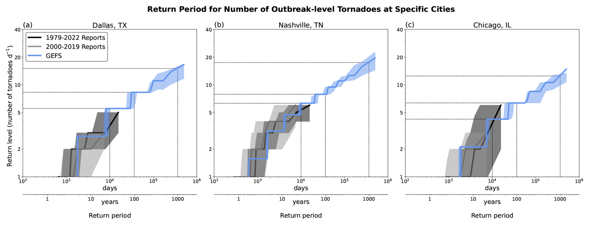
Figure 9 Return level curves for number of outbreak-level tornadoes per day from (black line) 1979–2022 reports, (gray line) 2000–2019 reports, and (blue line) GEFS synthetic event set for (a) Dallas, TX, (b) Nashville, TN, and (c) Chicago, IL. Shading indicates sampling uncertainty. Dotted lines highlight the 27-year return period level (to compare to Fig. 8) as well as the 100- and 1000-year return period levels.

4 Conclusions

U.S. SCS are an important driver of global insured losses, and tornado outbreaks cause localized destruction of life and property. Present-day risk assessment of U.S. tornado outbreaks using observations has limitations. Besides the relatively short record, reports have non-physical artifacts, and reanalysis environments describe only historical meteorological conditions, which may not represent risk from all physically possible and physically relevant meteorological conditions. Here we used GEFS, a rich dataset of physically possible but unrealized environments, to construct a synthetic event set for U.S. tornado outbreaks, and we demonstrate calculating present-day tornado outbreak risk statistics. At short leads, GEFS provides information on daughter events, which resemble the historical events, and, at long leads, GEFS provides information on physically independent yet realistic events. We estimated that the 1-in-100-year and 1-in-1000-year U.S. tornado outbreak event would have 150-250 and 275-400 (F/EF1+) tornadoes per day, respectively. In comparison, the observed reports can only resolve a 1-in-40-year event of ∼120 tornadoes per day with large uncertainty. We also estimated that the 1-in-10-year U.S. tornado outbreak annual total would have ∼450 tornadoes, well matching the estimate from reports. The GEFS synthetic event set represented similar La Niña-related increases in U.S. outbreak tornadoes per day during December–May season for more common (<1-year return period) events. It also represented similar increases in U.S. outbreak tornadoes per December–May season in the 2010–2019 period versus 2000–2009 period. In general, the GEFS synthetic event set more robustly detect trends in U.S. outbreak activity. Finally, we estimated location-specific information on tornado outbreak risk; the 1-in-1000 year event for Dallas, Nashville, and Chicago area is about 15, 17, and 12 tornadoes per day, respectively.

Because GEFS does not resolve tornadoes, we represented tornado activity based on GEFS environments and a tornado outbreak index. Therefore, using the GEFS synthetic event set for understanding outbreak risk for particular events relies on the tornado outbreak index performance in representing that event. Other indices or methods have been proposed to model severe weather in GEFS using its environments, though not specific to tornado outbreaks (e.g., Hill et al., 2020, 2023; Gensini and Tippett, 2019). The tornado outbreak index in this study performs well for most cases, and the average of events can be corrected relatively easily. However, errors in the distribution, e.g., what happens at the tails, are less easily corrected, so it may not work well for specific uses. Malloy and Tippett (2024, 2025) noted deficiencies in representing summer activity, i.e., likelihood is overestimated. In particular, in this study, we found that summer tornado outbreak events in the GEFS synthetic event set have higher variance and heavier right tails, i.e., extreme events happen much more frequently. Furthermore, the tornado outbreak index may not perform well in all SCS types or convective modes.

Another limitation is that, while the GEFS synthetic event set is very large, it has a limited representation of (multi-)decadal variability because of the relatively short number of years (2000–2019). Overall, the GEFS synthetic event set showed La Niña-related increases in outbreak activity, but the specifics of the shifts were dissimilar from reports (cf. Fig. 6. This period covers few ENSO events – 7 El Niño years and 8 La Niña years considering December–February ONI – and may not be representative of the diversity of ENSO events and its teleconnections (Deser et al., 2014). In addition, the general negative PDO and more La Niña months during this period might affect/skew the event set and, by extension, the trends (Franke et al., 2024).

The location-specific tornado outbreak risk was dependent on the parameters of the subsampling procedure. In general, the estimates from Figs. 8 and 9 may be underestimated with our subsampling procedure. The subsampling procedure “keeps” events based on user-defined thresholds in the mean/expected estimate of the total U.S. outbreak tornadoes as well as realizations from those events. This subsampling procedure uses a “keep” threshold based on CONUS-scale activity. While this is ideal for capturing the strongest events, we might be biasing the set by taking days with relatively high outbreak likelihoods, which usually represents events that occur over the Plains, Tennessee River Valley, Ohio River Valley, and southeast U.S. regions. Fewer samples are taken from “weaker” events, i.e., daily maps with smaller expected values but still have realizations where the event is considered an outbreak (>6 tornadoes), which may happen more in other regions, e.g., Northeast U.S. However, the subsampling procedure is designed to be flexible and user-defined, and future work can analyze other approaches to the subsampling. We also show that calibration of occurrence rates to match report data can help alleviate biases in GEFS. The calibration can also be flexible, e.g., users can define the occurrence rate from which to match the GEFS synthetic event set to reports.

In future work, the GEFS synthetic event set could include information on other important outbreak tornado characteristics, such as EF intensity and simulated tornado track. This can be modeled purely statistically or also be dependent on environments. For instance, Lepore and Tippett (2020) found that tornado intensity scaling was sensitive to SRH; SRH approximates potential for rotating updrafts, important for producing significant (EF3+) tornadoes. We also focused on outbreak tornadoes rather than both non-outbreak and outbreak tornadoes. While this work addresses assessing risk for the most rare, extreme events, it might not well resolve statistics for the typical, less extreme events. Future work could address physical constraints that are missing from this approach. For instance, the 100+ year return levels of tornadoes per day in Dallas, Nashville, and Chicago in Fig. 9 might not be physically realistic when storm-scale processes are considered. High-resolution models, e.g., High-Resolution Rapid Refresh (HRRR) model, could be used to determine physical constraints that limit how many tornadoes can occur in a grid cell per day, and storm-scale quantities used in short-term forecasting, such as updraft helicity, could provide insight into subgrid processes. The main drawback of using high-resolution forecast models is the relatively smaller ensemble sizes and forecast lengths, reducing the sample size and hence the spatial smoothness of risk maps. Overall, our approach is consistent with the use of large-scale environments, and while does not capture storm-scale processes, it has a major advantage of generating large sample sizes for estimating extremes.

Considering hail accounts for 50 %–80 % of SCS-related losses (Gallagher Re, 2024), a hail synthetic event set would also be valuable. Hail likelihood has a similar dependence on convective and kinematic environments as tornadoes, but the coefficients are likely to be different. For instance, Allen et al. (2015a) found that hail occurrence was more sensitive to CAPE compared to tornado occurrence. In Das and Allen (2024) study, extreme hail likelihood was generated using fitted extreme value models, a pure statistical approach. In addition, hail report data is more sporadic and might benefit from radar-based estimates of hail swaths (Brook et al., 2021; Fluck et al., 2021).

Finally, it would be valuable to combine this hazard risk assessment with estimates of exposure, or use exposure as a way to subsample events. In particular, the synthetic event set can be used to answer (re)insurance questions, such as calculating metrics like maximum probable loss or average annual loss from tornadoes, especially considering the GEFS synthetic event set estimates for annual tornado totals well matched report-based estimates (cf. Fig. 5). (Re)insurance or other loss data is often proprietary, but there are other ways to estimate exposure with available data. For instance, within the CLIMADA (CLIMate ADAptation) framework and project, their goal is to integrate hazard, exposure, and vulnerability to assess risk (Kropf et al., 2022; Stalhandske et al., 2024). The NASA VIIRS day-night band nighttime composites detects man-made sources of light and – when combined with population data – can estimate exposure (Eberenz et al., 2020). In addition, U.S. crop loss data is provided by the United States Department of Agriculture. In general, this GEFS synthetic event set is a valuable dataset for assessing tornado outbreak statistics and risk.