The quest for reference stations at the National Observatory of Athens, Greece

The assumption of reference station conditions is investigated for the first time across 60 rock stations belonging to the broadband and accelerometric networks of the National Observatory of Athens. We include in our assessment all stations that have some probability of lying on rock, based on existing data or beliefs, provided their data have been publicly available for long enough to yield a substantial number of recordings. No studies on site effects have been conducted before for the ensemble of stations. Furthermore, almost no ad hoc field campaigns have been performed to characterise them. The first step is to compile all readily available information per station from publicly available external sources, i.e. geology, topography, housing, Vs₃₀ estimates, and any other known metadata. The second step is to analyse geological maps to derive the geological unit and age; to combine this external information with internal information (namely questioning network staff to access the operator's first-hand experience of the sites); and to better describe geology, geomorphology, and station installation details. The third and largest step is to compile the first Greek ground motion dataset on rock and to perform a detailed analysis of the recordings to estimate site-specific amplification to assess the local site response for each station. A strong-motion dataset of over 7500 recordings is developed and curated for this purpose, dating from 2012 to 2023. It is visually inspected and meticulously processed on a waveform-specific basis in the time and frequency domains, paying special attention to signal quality and strength. Single-station amplification functions using horizontal-to-vertical spectral ratios (HVSRs) are then estimated from the database. Considering that “true” reference sites should have low, flat amplification with no directional dependence, the analysis goes beyond the usual path of combining the two horizontal components into a mean HVSR. It also assesses the directional sensitivity of the HVSR to identify departure from the 1D assumption, corrects the HVSR for the vertical amplification effect, and uses clustering techniques to select groups of stations with different response characteristics. This data-derived characterisation is combined with the previously compiled station metadata to evaluate the stations' overall capacity as reference sites. This results in a qualitative ranking of the stations. The least and most adequate reference stations are showcased to facilitate a better use of seismic data in future seismological and hazard applications.

1 Introduction

1.1 The need for station characterisation and reference stations

The importance of understanding site conditions at strong-motion recording stations, which often lie on soft soils, has been known for decades. Important global databases such as NGA-West2 (Ancheta et al., 2014) have made a point of procuring rich and homogeneous station metadata in terms of shear-wave velocity (Vs), depth to bedrock, etc. Ground motion models have moved towards more detailed descriptors of station conditions, and a global effort is being made in characterising strong-motion stations. On the contrary, permanent seismological stations are typically installed at rock sites and are assumed to be free of any site effect, so there is rarely any effort to characterise them or challenge their quality as reference stations. Recently, strong-motion and broadband seismological data have been used together more often as the limits between the different sensor capabilities begin to blur and magnitudes of interest decrease. Hence, it is a good time to ask the question of whether the scrutiny traditionally applied to strong-motion station conditions may also now be applied to seismological stations.

In the past, ground motion on rock sites was regarded as mostly homogeneous with no amplification; some notable exceptions include the seminal works of Silva and Darragh (1995) and Steidl et al. (1996). Nowadays it is more widely recognised that material property and geometry variations can affect rock ground motion as well, likely at higher frequencies. This has a potential impact on reference ground motions and the definition of reference stations, which were once simply defined as those coming from “rock” sites. It has already affected seismic hazard and risk assessment for significant structures and critical infrastructures where rock property variations are accounted for in detail. However, rock sites can be notoriously challenging to characterise, and many networks have not characterised theirs, as priority is given to stations lying on soil.

Some studies in the past decade or so have focused on rock sites. Van Houtte et al. (2012) tested stations in Christchurch that were typically used as reference stations without previous checks by computing site transfer functions. Ktenidou and Abrahamson (2016) found broadband amplifications in CENA rock sites that had been regarded as extremely hard (Vs₃₀ of 2000 m s⁻¹). More recently, systematic and large-scale efforts have been made at the European level by Lanzano et al. (2020), who defined reference sites in central Italy using various proxies and transfer functions from seismic data and noise, while Pilz et al. (2020) also included artificial intelligence tools in their reference site identification. Di Giulio et al. (2021) systematically assessed seismic station characterisation efforts across Europe in terms of data quality, methodological reliability, etc., emphasising the importance of consistency.

1.2 Motivation of this study

The new European Seismic Hazard and Risk Models, also known as ESHM20 (Danciu et al., 2021) and ESRM20 (Crowley et al., 2021), were published recently. The latter includes an empirical amplification model based on Vs₃₀ at the European scale (Weatherill et al., 2023) to account for site effects with respect to rock conditions. In Greece, Pitilakis et al. (2024) recently proposed a new seismic hazard zonation map for potential consideration in the new national annex to accompany Eurocode 8 (EC8; CEN, 2004). The zones were defined with respect to rock conditions in order to be used for seismic actions in different geotechnical/geological contexts. From the EC8 point of view, Labbé and Paolucci (2022) reported that the new site classification draft included not only amendments to soil classes, but also an additional parameter to define rock class, namely the fundamental frequency. The definition of soil conditions is relevant to the definition of rock, and the latter is acquiring prominence. A large scope of models and applications is affected by such definitions, including ground motion models, seismic hazard maps, and ShakeMaps. Hence, it is a good time to consider the question of reference sites.

Although Greek data are important to European and even global ground motion datasets, relatively little progress has been made in the digital era in characterising stations. Many reasons lie behind this, including the fact that significant numbers of seismic networks are run by different operators (Evangelidis et al., 2021) and that large numbers of stations are off the mainland or in areas that are difficult to access. Some efforts have been made to compile station metadata since the early days of HEAD, the first strong-motion database (Theodoulidis et al., 2004). Margaris et al. (2014) provided a brief history of the characterisation of Greek strong-motion stations with boreholes, geophysical campaigns, and microtremors, while Stewart et al. (2014) compiled values of Vs₃₀ and other site descriptors for some strong-motion stations, mostly based on information within a 1 km radius from the stations. Margaris et al. (2021) include the most up-to-date version of available strong-motion station metadata, mostly through proxies. We note that the above studies include a large number of stations on soft ground, and some of them are not yet publicly available through European waveform services (Engineering Strong Motion (ESM) Database). Systematic effort has been made for one of the Greek networks (HI, https://doi.org/10.7914/SN/HI; ITSAK, 1981) by Grendas et al. (2018), where the actual strong-motion recordings were analysed to compute empirical transfer functions.

The goal of this work is to focus on the network of the National Observatory of Athens (network code HL, https://doi.org/10.7914/SN/HL; NOA-GI, 1975), including not only the strong-motion stations (channel code HN, https://accelnet.gein.noa.gr, last access: 31 December 2023) but also the broadband seismic stations (channel code HH, https://bbnet.gein.noa.gr/HL/, last access: 31 December 2023) that are openly available in real-time continuous mode through the EIDA@NOA node (Evangelidis et al., 2021). Site conditions are known in great detail for a fraction of the strong-motion stations thanks to geophysical in situ investigations conducted in the recent national Hellenic Plate Observing System (HELPOS) project; however, most of these stations lie on soils. To date, most available strong-motion stations are still characterised via proxies, and none have been analysed to determine empirical amplification functions via earthquake recordings. Moreover, there has never been a systematic effort to include broadband stations, despite the increasing importance of broadband data in ground motion databases. In the HL network, only a few small-scale efforts were made recently to understand the behaviour of selected strong-motion (HN) and broadband (HH) stations using the recordings themselves (Ktenidou and Kalogeras, 2019; Ktenidou et al., 2021a, b). These used limited datasets, mostly as proof of concept. This paper marks the beginning of a more systematic study of the NOA network conditions, starting with rock sites.

2 Strong-motion data and analysis

2.1 Station and data selection

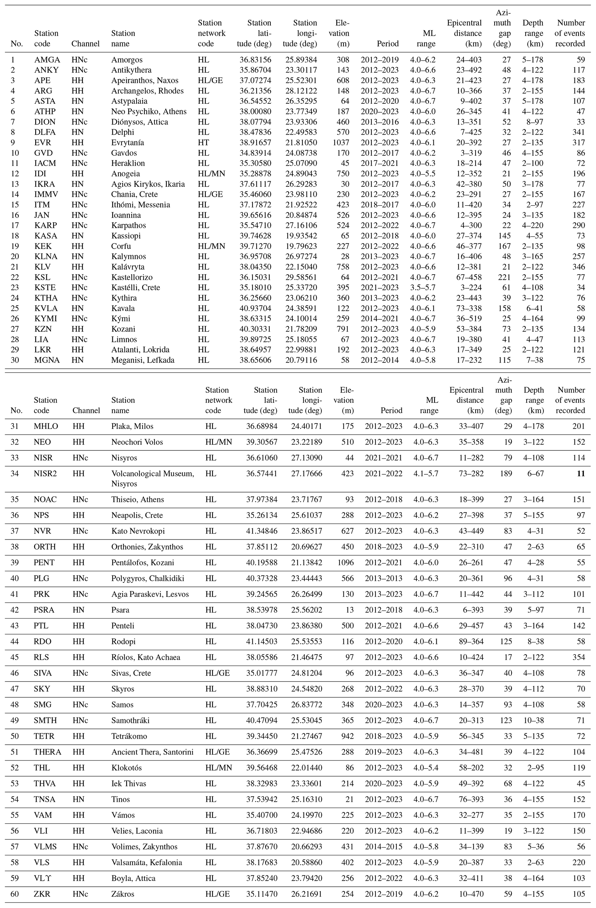
Stand-alone broadband stations (HH channels) and collocated broadband and strong-motion stations (HH and HN channels) are generally assumed to lie on rock. Hence all these stations are included in this study, as long as they had enough recordings at the end of 2023, which could be publicly accessible via the EIDA@NOA node at that time (Evangelidis et al., 2021). In addition, we considered all stand-alone strong-motion stations (HN) open via EIDA and selected those for which some indication existed of them lying on rock. Such indications included literature and online resources, geological map information, proxy-based information, operator's information, and site visit information. The rationale behind this selection process was simple: we would rather include more stations than are actually reference sites and dismiss them later after detailed scrutiny than miss out on potential reference stations due to strict initial criteria. The stations selected are shown in Fig. 1, and some basic information about them is compiled in Table 1 (“HNc” indicates strong-motion stations installed at the same site as a broadband station).

Table 1 General information and metadata for the stations in this study and statistics on the ground motion data analysed.

A threshold minimum magnitude of M_L 4 was considered, dropping to M_L 3.5 only in one case, for a station installed in 2021. The maximum distances considered varied according to noise level and scales from 150 km for smaller events to almost 500 km for large events. The M–R distribution for the ensemble dataset is shown in Fig. 2a. Figure B1 of the Appendix shows the M–R distribution for all stations in alphabetical order. Because the purpose of this dataset is not the development of ground motion models, the M–R distributions are given as an indication only, and we use local magnitude and epicentral distance metrics without giving the moment magnitude or rupture distance for large events. A total of 7512 three-component recordings are analysed in this study, coming from 1364 earthquakes. The number of three-component records per station is shown in Fig. 2b and is also listed in Table 1 as number of events recorded. The minimum number of usable recordings is 11, and the mean number of recordings is 125, although some stations have more than 300.

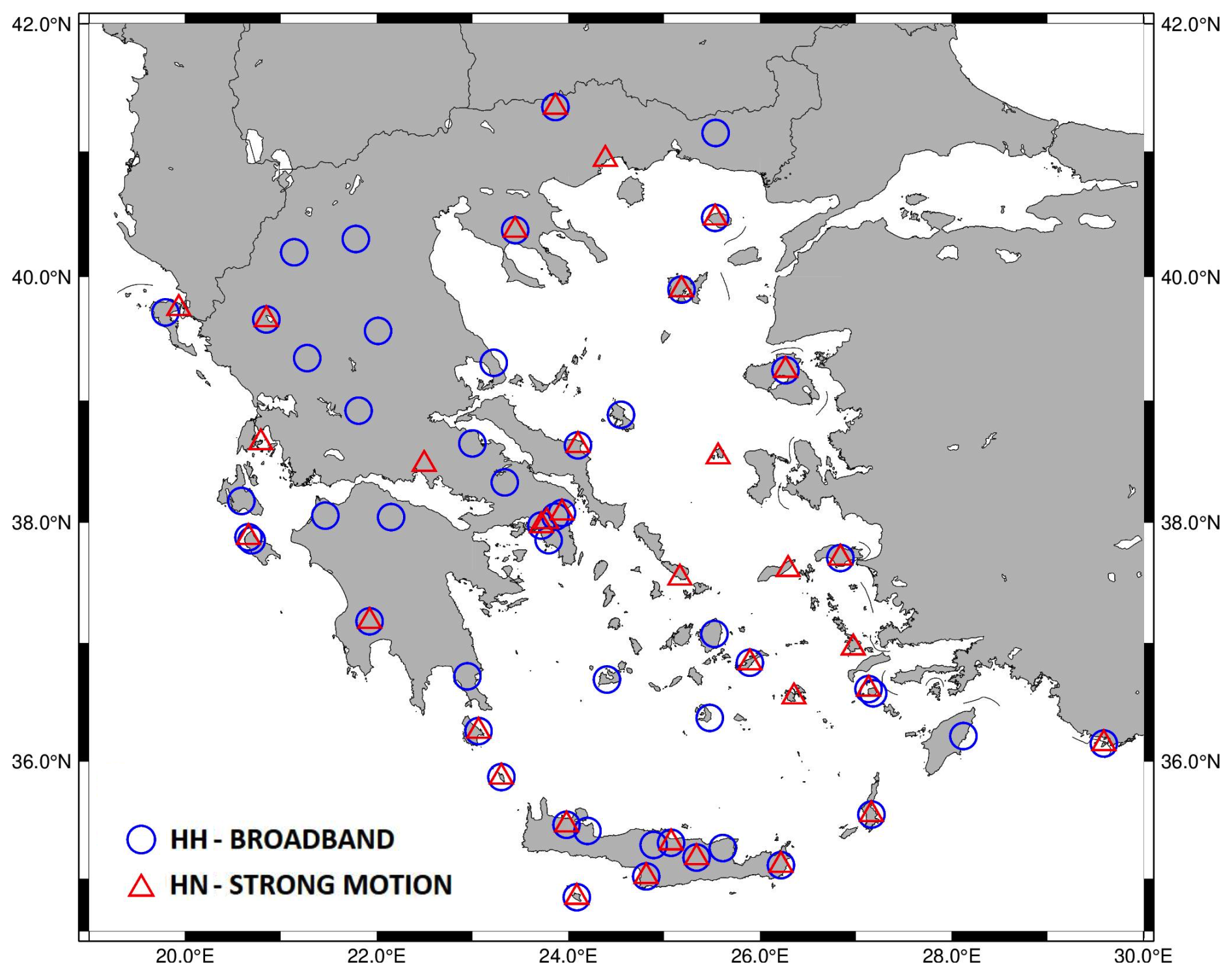
Figure 1 Map of selected HL stations (believed to lie on rock, with publicly available data via EIDA@NOA and an adequate number of events).

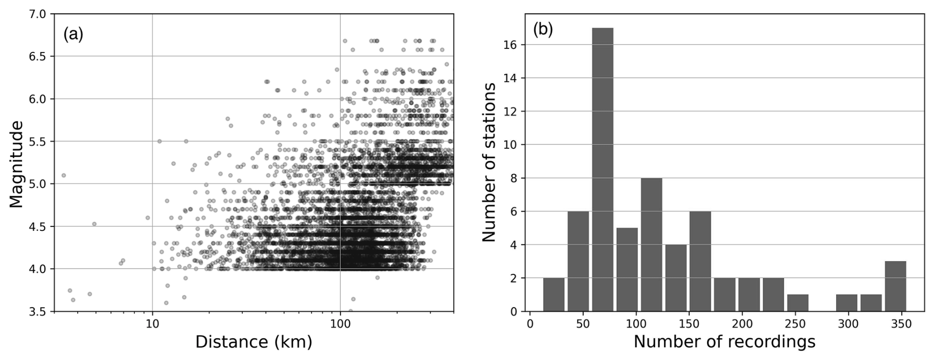
Figure 2 (a) Indicative distribution of magnitude (local) and distance (epicentral) for all recordings analysed in this study. Station-specific M–R plots can be found in the Appendix (Fig. B1). (b) Histogram of the number of recordings used per station.

2.2 Data processing and creation of a new strong-motion dataset

The data we select come from the period 2012–2023, depending on operation time and data availability per station. We use the catalogue of NOA (https://eida.gein.noa.gr/fdsnws/availability/1, last access: 31 December 2023) and search for recordings following the criteria mentioned above. We retrieve raw waveforms and station XML from EIDA@NOA and apply instrument correction to retrieve physical units. We then develop a data processing workflow inspired by that of Kishida et al. (2016), which underpins NGA-East (Goulet et al., 2014). Our procedure differs from manual processing protocols elsewhere, such as the European services (ESM Database; Lanzano et al., 2021; Luzi et al., 2016), because here comparison of signal quality with respect to noise at both high and low frequencies is paramount. We develop our own in-house software for analysis in the time and frequency domain, whose main steps are described below:

1. We check raw broadband (HH) data for clipping and discard all such instances. This is not relevant for strong-motion (HN) data.

2. We perform visual inspection on all instrument-corrected waveforms in the time domain to discard obvious problematic cases (low quality, component errors). We treat double events (two earthquakes occurring one right after another, leading to interference of the various wave packages) on a case-to-case basis, salvaging data where possible.

3. We perform windowing based on expected P and S arrival times that are first automatically computed based on the origin time and location of each event. S-wave duration is estimated based on magnitude and distance, and an equal duration is chosen for the pre-event noise window.

4. Expected window markers are first plotted on the seismogram as dotted lines (Fig. 3 – top), and the analyst assesses and amends them as needed (solid lines). Note that we aim for the signal window to include all wave packages of engineering interest, i.e. all S waves and the most energetic surface waves. Appropriate allowances are made for the tapering not to affect S arrivals.

5. Pre-event and signal windows are cut and tapered before computing Fourier amplitude spectra (FAS) of acceleration. We smooth FAS using the Konno and Ohmachi (1998) window with a mild b=40. We compute the signal-to-noise ratio (SNR) on the smoothed FAS for each component. However, for low frequencies the SNR is not necessarily a good indicator because of the small number of points; hence we rely heavily on visual inspection of the FAS.

6. We visually inspect the frequency domain, assessing both smoothed and unsmoothed acceleration FAS of the signal, the noise, and 3 times the noise spectra, in log and linear scale respectively (Fig. 3 – middle and bottom). In addition to the signal-to-noise ratio (SNR = 3 threshold), we also consider the fit of the omega-square source model (Brune 1970, 1971) in the low-frequency band.

7. We select the lowest and highest usable frequencies (LUFs and HUFs). We work in the frequency domain so we need not filter between them, but we take great care that each Fourier amplitude spectrum used to compute empirical transfer functions in the next step is used strictly within its usable frequency range. This way, the results are reliable, and we believe that they carry no noise-related artefacts.

This leads to the creation of a new database of over 7500 three-component recordings that includes the hand-picked usable bandwidths of all recordings of events > M4 at the 60 potential reference stations of the HL network that were available until the end of 2023. Thanks to the care exercised in selecting the corner picks, this database can be used with confidence by those seeking to exhaust the usability of recordings at the low and high ends of the spectrum.

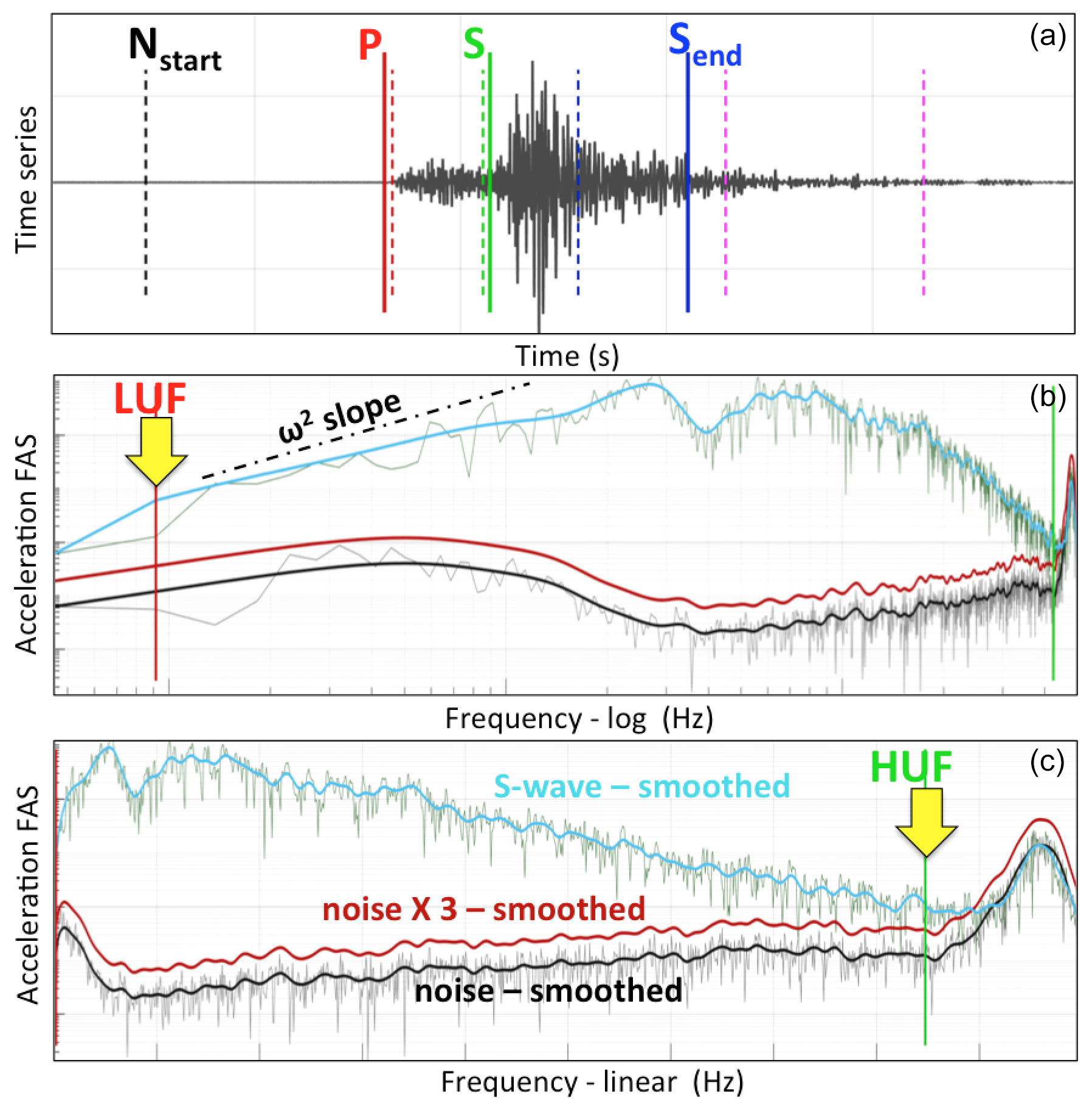
Figure 3 Example of manual processing. (a) Windowing of a velocity trace in the time domain, selecting the beginning of the noise and S windows and the end of the S window. (b, c) Selecting the lowest and highest usable frequencies (LUFs and HUFs) in the frequency domain in log and linear scales respectively on the acceleration FAS.

3 Empirical transfer functions

3.1 Orientation-independent HVSR

We compute the horizontal-to-vertical spectral ratio (HVSR; Lermo and Chávez-García, 1993) for each horizontal component of each recording at each station. We compute the spectral ratios in the same manner as the SNR: the start of the S-wave window is chosen so that the S waves are not affected by the tapering, and the acceleration FAS are computed and smoothed with a Konno and Ohmachi (1998) b=40. The mean HVSR per site is computed as the logarithmic average of all events, as is customary, and given that Ktenidou et al. (2011) showed that empirical spectral ratio ordinates are lognormally distributed. At each frequency, the mean is computed using recordings strictly within their legitimate bandwidth (from LUF to HUF), so the contributing number of earthquakes varies with frequency. Within the range of 1–10 Hz, typically all recordings are usable, while towards lower and higher frequencies, fewer recordings are strong enough to contribute. The FAS of the two horizontal components are combined for each recording as the square root of the sum of squares (SRSSs) to yield an orientation-independent estimate. Figure 4 (top) shows two examples of this rotation-invariant mean HVSR ± 1 SD. The inset on top indicates the number and percentage of usable recordings per frequency; e.g. for the APE station, 183 earthquakes contribute to the HVSR in the range of 0.9–9 Hz and less than 25 % (46 earthquakes) at frequencies below 0.07 Hz and above 25 Hz. The curves and their ± 1 SD uncertainty (shaded area around the mean) are only drawn for frequencies where the number of usable events is at least 5, to ensure a more robust estimate (many ground motion applications require 3). Figure B2 in the Appendix shows the rotation-invariant mean HVSR results for all of our 60 stations in alphabetical order. Figure 4 (bottom) is explained in the following section.

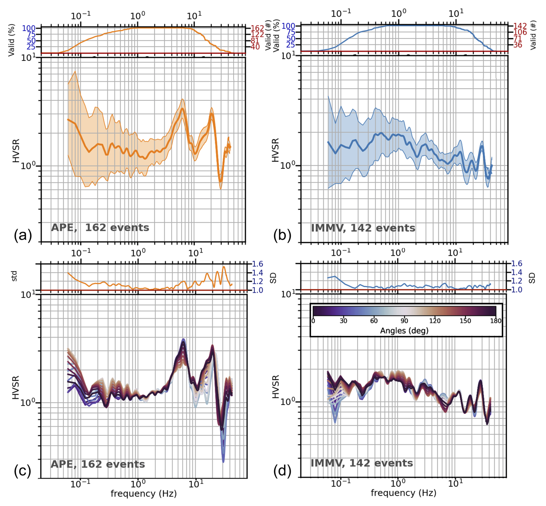
Figure 4 Example of HVSR results for stations APE (a, c) and IMMV (b, d). (a, b) Mean, orientation-independent (SRSS) HVSR ± 1 standard deviation; the inset on top indicates the number and percentage of usable recordings per frequency. (c, d) HVSRs per component, as those are rotated 17 times by a 10° interval, from north to south; the inset on top indicates the standard deviation (hence, directional sensitivity or variability) per frequency.

Let us now study the shape of the HVSR in Fig. 4 (top). A reference site is expected to exhibit an HVSR that is relatively flat and close to unity. Significant departure from reference site conditions has been judged in different ways. Some studies consider a minimum threshold value of HVSR > 2, while others consider HVSR $>\mathrm{2}\surd \mathrm{2}=\mathrm{2.8}$ (Lanzano et al., 2020, from Puglia et al., 2011) or even HVSR > 3 (Pilz et al., 2020). HVSR is an approximation and is generally considered to underestimate the “true” site transfer function with respect to the standard spectral ratio (SSR) of Borcherdt (1970), i.e. using an actual rock recording as reference rather than the vertical. The premise of HVSR is not necessarily that the vertical component remains unaltered by stratigraphy but rather that it is expected to amplify frequencies higher than those of the horizontal components (typically at √3 times the resonant frequency of the horizontal S waves). Thus, it permits a clear identification of at least the first resonant peak of the S waves, albeit at an underestimated amplitude.

In our case, the value of 2√2 as the minimum threshold to identify amplification on the HVSR is mathematically more appropriate, given that we computed the SRSS of the two horizontal components (corresponding to the hypotenuse of the two orthogonals, N and E). Therefore, we use a threshold of HVSR $>\mathrm{2}\surd \mathrm{2}$ when identifying significant resonant peaks and a threshold of HVSR < 2 when selecting potentially adequate (relatively flat) reference sites. Based on this rationale, station APE in Fig. 4 (left) exhibits a clear resonance at 6 Hz with an amplitude larger than 2.8, followed by a likely first higher mode at roughly 3 times that frequency, 20 Hz. This resonance is far from the desired behaviour of a reference site. On the other hand, station IMMV in Fig. 4 (right) has a rather flat HVSR with an amplitude of < 2, indicating a potential reference site. Similar results are shown for all of our 60 stations in the Appendix (Fig. B2). After consideration of all stations, Fig. 5 shows the most likely reference sites, with the HVSR being flat over a wide frequency range and < 2. Conversely, Fig. 6 shows the least adequate reference sites, with non-flat HVSR shapes and amplitudes exceeding 2.8 over a narrow or broadband frequency range. Table A1 in the Appendix compiles the resonant frequencies (f₀) and their corresponding amplitudes (A₀) thus identified. As a comparison, it also shows the f₀ identified automatically by a picker. The table also includes the first higher mode (f₁, A₁) for the few cases where they were clearly identified. HVSR being only a proxy, it is conceivable that an inadequate reference station may show a flat-shaped HVSR, but it is expected that an adequate reference station shows a flat HVSR.

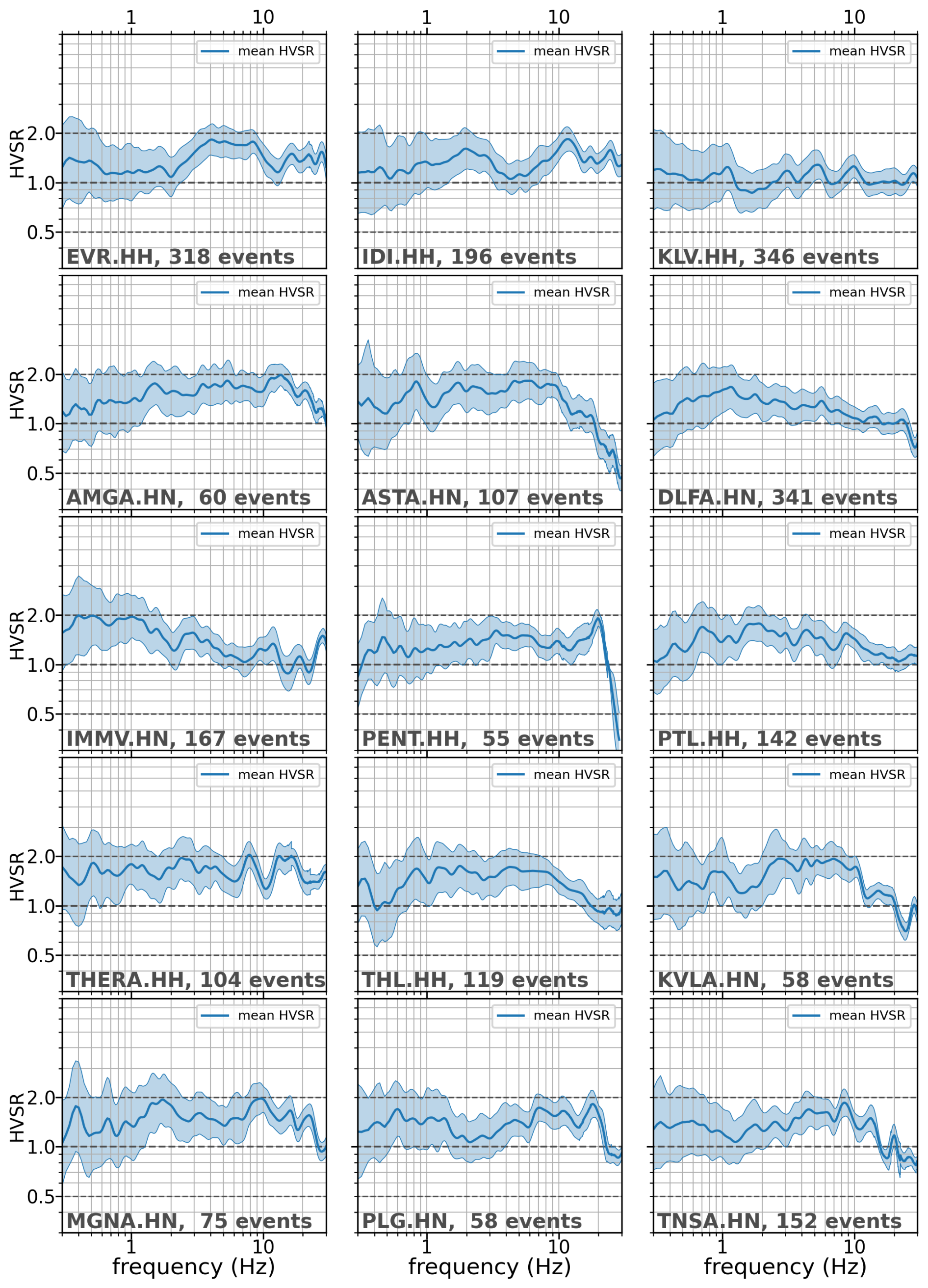
Figure 5 The most adequate HVSR shapes, flat over a wide frequency range with amplitudes smaller than 2.

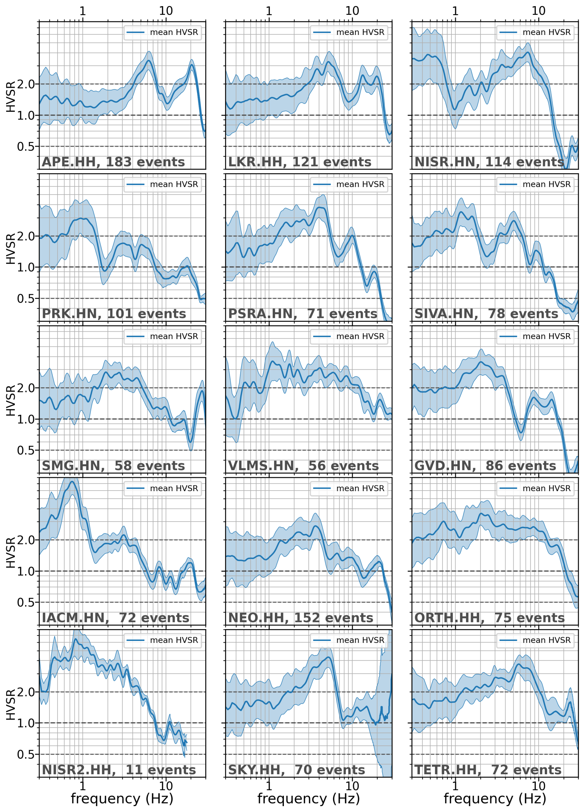
Figure 6 The least adequate HVSR shapes, with non-flat shapes and amplitudes exceeding 3 over a narrow or broadband range.

3.2 Rotational sensitivity of HVSR

A reference site should not exhibit strong directional dependence; i.e. reference ground motions should not be sensitive to the sensor orientation, at least in the frequency range of interest to each application. However, checking only the difference between the two horizontal components as installed can be a somewhat random way of accounting for such effects because the sensors are installed in the N and E directions, which are actually arbitrary with respect to each site's potential geomorphological features. This is why we follow the technique of Ktenidou et al. (2016) to assess the variability of site response to azimuth. We rotate each time series by successive increments of 10°, from 0–90°, and recompute the FAS and HVSR each time (yielding a total of 18) to investigate directional differences. We view these as an indication of departure from 1D behaviour because if there is orientation dependence, it is likely due to and aligned with the direction of the local geomorphological features of the site (basin edges, inclined layering, lateral discontinuities, topography, etc.), e.g. the radial and transverse with respect to the feature's axis. For example, Ktenidou et al. (2016) used successive rotation to show that the maximum and minimum amplification level observed near a basin edge occurred in directions parallel and perpendicular to the basin edge axis respectively.

Figure 7 shows an example of how directionality is quantified. The mean HVSR is computed per component as it is rotated by 10° increments; e.g. the north component is rotated from 0–170° in order to sample all possible orientations. The inset on top indicates the standard deviation per frequency of HVSR values across all angles. We consider this standard deviation (SD) value to be an index of the directional variability of each station's site response. The typical parameters extracted from such calculations are the resonant frequency f₀, the corresponding amplitude A₀ – mostly as an indication – and the same metrics for the first higher mode, if applicable. In addition, we note the directional variability (SD) of the transfer function amplitude, and to this end we compute the mean of the SD function across two indicative frequency ranges of interest, namely a wide one spanning 2 orders of magnitude (0.3–30 Hz) and a narrow one perhaps more interesting for typical structural response (1–10 Hz). We also note the value of this function around the resonant frequency of the site. We propose that these three values (SD_0.3−30, SD₁₋₁₀, SD_fo) can be used as approximate indicators of the azimuthal stability of site response. For site VLS used as an example in Fig. 7, the scatter in HVSR occurs above 10 Hz and thus affects mostly SD_0.3−30 (1.24) and SD_fo (1.48 at 20 Hz), while SD₁₋₁₀ (1.12) is relatively low.

The bottom line of Fig. 4 shows the relevant results, which we can now compare to the orientation-independent mean HVSR in the top line. We observe that station APE, which had already been judged poorly due to its clear strong peaks above 3 (top plot), is now seen to also exhibit non-negligible directional variability around its f₀ of 6.1 Hz of 1.20 (bottom plot). In contrast, station IMMV appears to be a very good candidate for a reference site, with no identifiable peak (top) and also low directional sensitivity of 1.07 (bottom).

Figure 8 illustrates a few characteristic examples of HVSR shape and directional sensitivity. Considered in the 0.3–10 Hz band, ASTA is the best candidate reference station with no amplification and very low SD, followed by VLS, with higher variability (yet still acceptable below 10 Hz). VLI exhibits a weak but clear low-frequency resonance, while IACM shows a clear strong fundamental peak followed by a clear first higher mode. None of these two stations show directional variability. KTHA and NISR2, on the other hand, show small and large peaks respectively, which are broadband (not as “peaky” as their counterparts VLI and IACM), and in addition possess very high directionality. The behaviour of most of these stations is certainly not what we would expect of rock stations. Based on geological labels indicating rock or the fact of being seismological stations, one might be inclined to regard them a priori as reliable reference stations. Nonetheless, we observe cases of either low-frequency (IACM, NISR2) or high-frequency (VLS) amplifications of up to 6–8. In addition, for a value of SD > 1.20, the reference ground motion would depend strongly on sensor orientation, up to factors of 2 or 3 at certain frequencies. Figure B3 in the Appendix shows the directional dependence for all 60 stations in this study. Table A1 in the Appendix also includes columns related to the sensitivity (SD values and qualitative descriptions). After considering all cases, we believe that an SD value less than 1.06 is low, more than 1.15 is high, and more than 1.20 is very high.

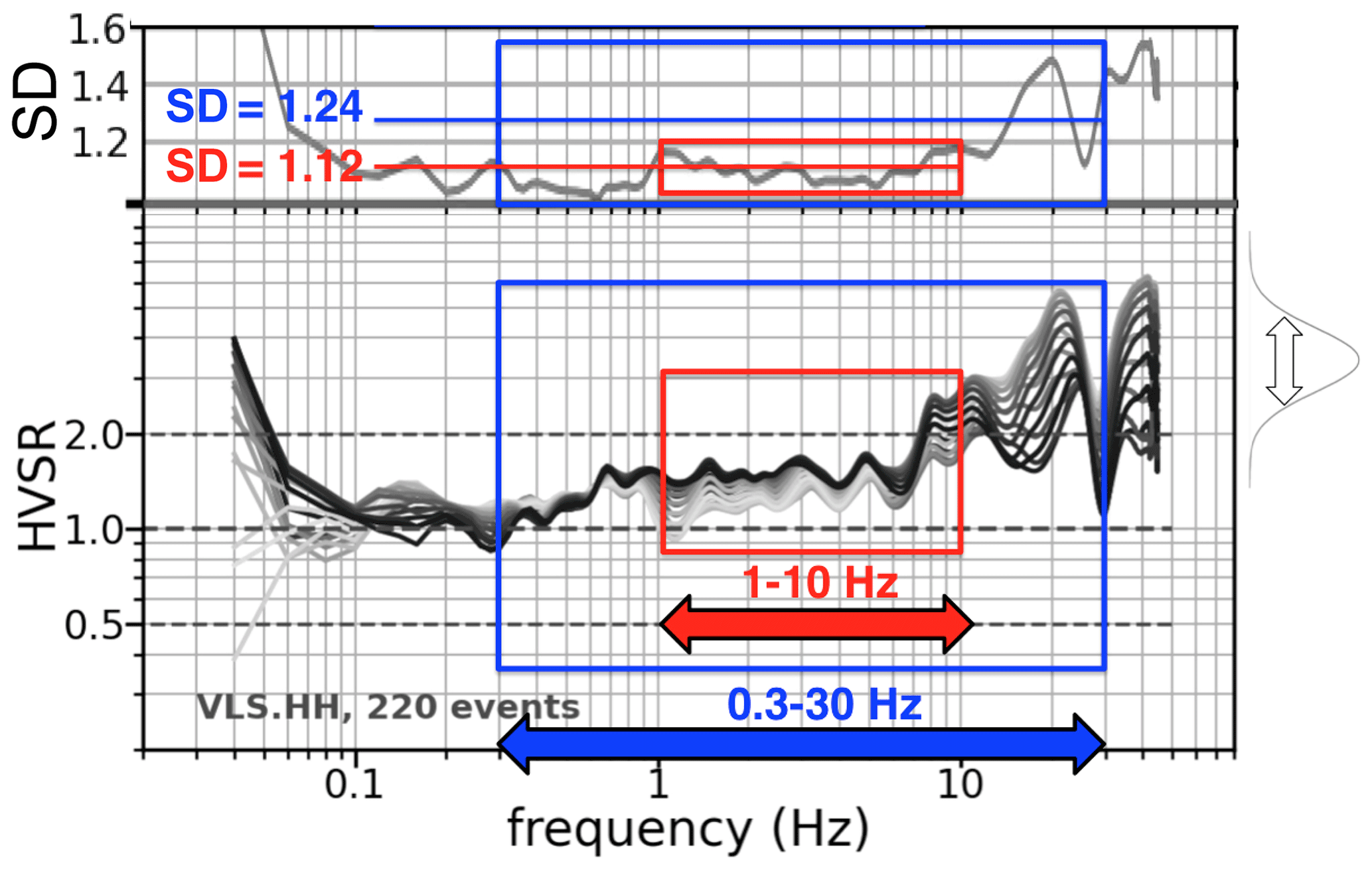
Figure 7 Illustration of the two frequency bands over which the standard deviation from the rotations is averaged to derive an index of directional variability: 0.3–30 Hz (blue) and 1–10 Hz (red). For station VLS, the value is low for the narrow band (1.12) but high for the wider one (1.24) due to high-frequency variability above 9 Hz.

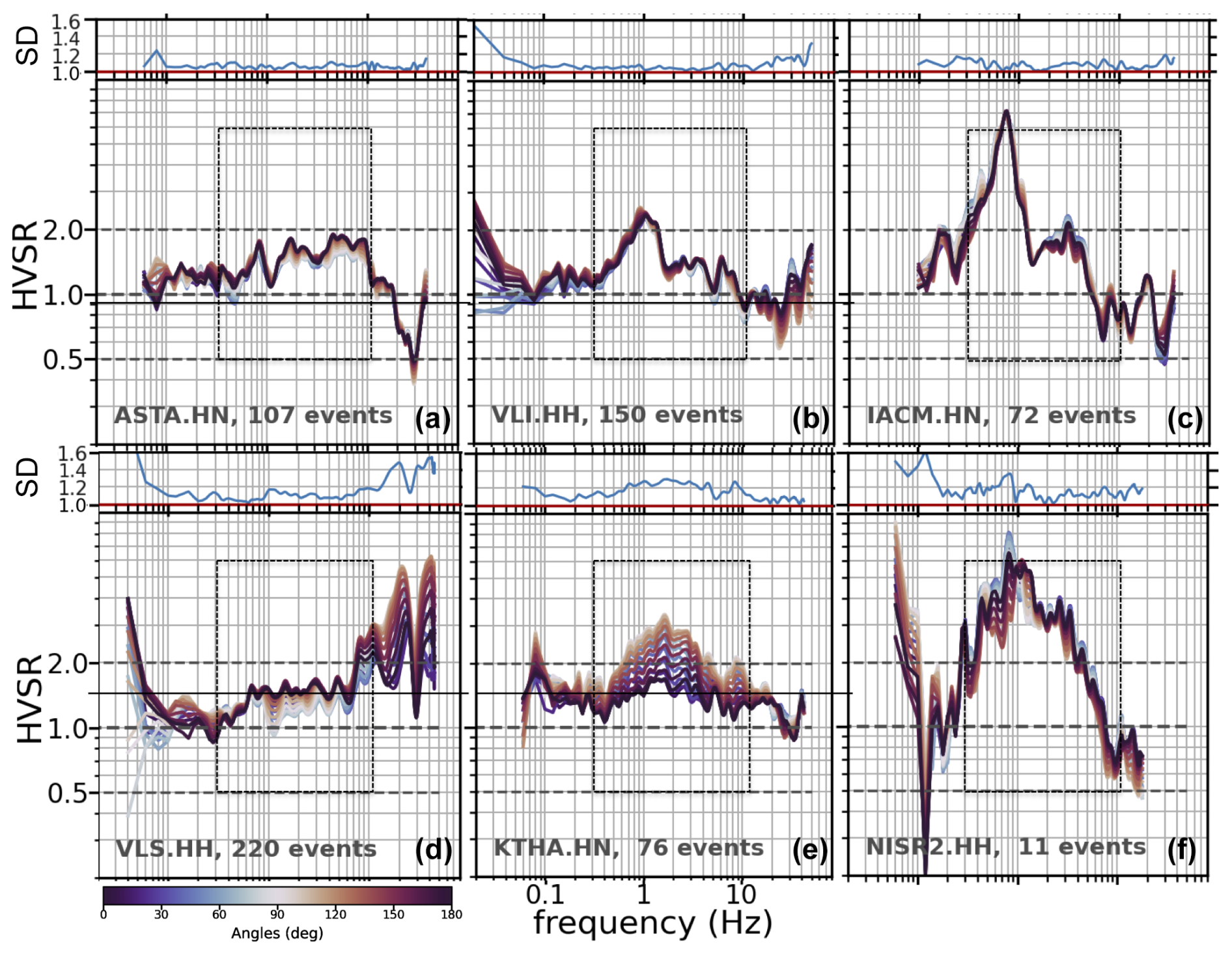
Figure 8 Indicative examples of HVSR: (a, d) low, (b, e) medium, and (c, f) high amplification within the range of 0.3–10 Hz, showing (a–c) lower and (d–f) higher variability with azimuth.

3.3 Correction of HVSR for the vertical component

The HVSR is but a proxy for the actual amplification level (as given e.g. by the standard spectral ratio (SSR) of Borcherdt 1970), partly due to potential amplification of the vertical component used as reference. To investigate the extent of the potential underestimation in amplitude level, as an experiment we perform an additional calculation: we correct the HVSR for the implicit amplification of the vertical component. Because there is no model for Greece, we use the vertical amplification correction function (VACF) developed for Japan by Ito et al. (2020). The authors proposed this as a simple tool to estimate the horizontal S-wave amplification from the HVSR. It is based on diffuse field theory and their results from applying the generalised spectral inversion technique (GIT) to assess vertical site amplification from over 1600 strong-motion sites in Japan. Ito et al. (2020) proposed VACFs for various site classes based on HVSR shape, which are relatively constant in the frequency range of 1 to 15 Hz with an average amplitude of about 2. Applying this Japan-based method to Greek stations of course has its limitations, but in this experiment we consider that it may be a useful first approximation, as it comes from a region with a similar (active) tectonic regime. Considering that it is in any case a mere average over thousands of sites, individual site characteristics are already blurred. The VACF is proposed for 0.12–15 Hz, so we constrain our corrections to this range of applicability. An example comparison of HVSR and its VACF-corrected version is shown in Fig. 9 for the two stations shown previously in Fig. 4. For station APE (left), the 6 Hz resonant peak already identified by inspection of the mean HVSR becomes even more prominent after the VACF correction, with the amplification doubling from 3 to 6. On the other hand, at station IMMV (right), where HVSR did not exhibit enough amplification to identify significant peaks, a peak becomes visible at 1 Hz after VACF correction.

Figure B4 of the Appendix shows the comparison of HVSR and VACF-corrected HVSR for all 60 stations of our dataset. It aims at giving an idea of the possible amplification level out to 15 Hz, but we note that these results are mere approximations and carry the inherent shortcomings of HVSR, Japan-derived VACF, etc. For instance, an unexpected amplification of the vertical component will map onto the horizontal. Table A1 in the Appendix includes A_{0_corr} (the maximum amplitude A₀ after VACF correction) and in a few cases the newly identified resonant frequencies (f_{0_corr}) with their corresponding amplitude. We offer field A_{0_corr} only as a rough indication of possible absolute amplification level. Finally, we note that another source of uncertainty could be nonlinearity in the recordings, although this is not very probable for rock/stiff conditions.

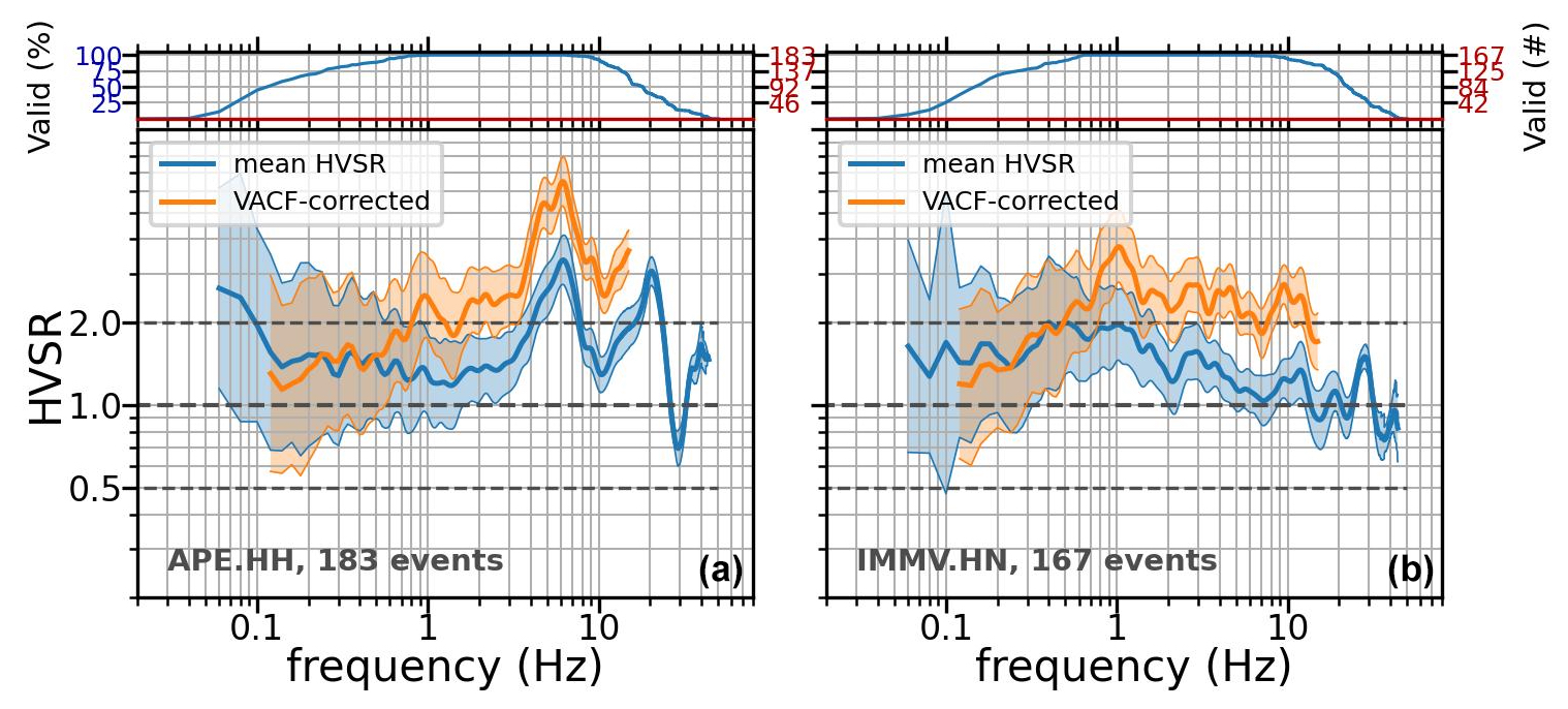
Figure 9 Comparison of mean HVSR ± 1 SD (blue) with the VACF-corrected HVSR (orange) using the Ito et al. (2020) vertical component correction function at the same two stations shown in Fig. 4. (a) A pre-existing peak is doubled. (b) A new peak becomes visible.

3.4 Clustering

We consider the results across the 60 stations together and group them into categories or clusters. To this end, we use hierarchical agglomerative clustering on the mean, orientation-independent HVSR. Agglomerative clustering starts by having each observation in its own cluster (of size 1) and builds a cluster hierarchy by iteratively merging the closest cluster pair at each step. The resulting hierarchy (also called a dendrogram) is pruned at a suitable level either by defining a maximum inter-cluster distance or by specifying the desired number of clusters. Agglomerative techniques are differentiated by the way they define the similarity (or linkage) between two clusters (i.e. sets of observations). For example, “complete” linkage defines similarity as the maximum of all pairwise distances between participants of the two clusters, while “single” linkage defines it as the minimum distance. In our case, after experimentation, we selected the Ward criterion (Ward, 1963) as the linkage method, seeking to minimise the intra-cluster variance of the cluster created. We used the Euclidean distance as the distance metric and the scikit-learn library as our tool.

Figure 10 Groups of stations with similar amplification based on mean HVSR.

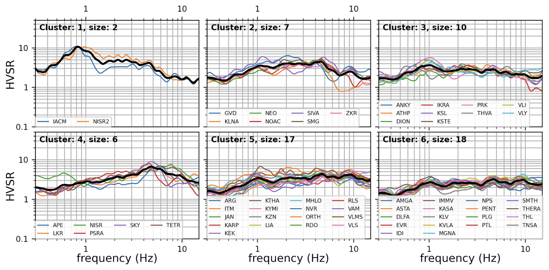
Figure 10 shows the six clusters derived from analysis of the HVSR curves. Cluster 1 shows clear low-frequency (LF) resonance for two sites, cluster 4 shows high-frequency (HF) amplification for six sites, and cluster 2 shows broadband amplification for seven sites. These three categories would not be considered to be reference sites. Cluster 6 includes 18 reference sites. Clusters 3 and 5 show low amplification with a downtrending and flat shape respectively, so they could likely be acceptable reference sites. The main classes identified by this analysis can be roughly distinguished as reference stations, LF/HF/broadband amplification that makes the response deviate from a reference site, and smaller amplification patterns that do not deviate strongly from the flat response. Other groupings could be reached by constraining the algorithm parameters, but our goal here is to call attention to a few patterns and how/if they deviate from the expected (flat) rock response. Finally, as an experiment, we repeat the clustering on the VACF-corrected HVSR, and the results are shown in Fig. B5 of the Appendix. Figure B6 of the Appendix compares the mean cluster shapes for the two cases. Table A1 of the Appendix includes the cluster number per station according to both groupings and a qualitative description.

We do not investigate what lies behind the amplification pattern we observe at each individual station. As the stations are generally considered rock sites, in what follows we only mention a few possible reasons – other than geological misclassification – that could explain HVSR peaks on rock. Sharp high-frequency peaks can be due to shallow, near-surface soft or weathered layers on bedrock (Ktenidou, 2022). Their amplification level will increase with the impedance contrast between the two materials. A directional dependence of an amplification peak could signify 2D or 3D site effects. A low-frequency low peak could indicate a deep interface between soft and harder rock. Another possible reason behind rock site amplification is topography, which would be expected to take place at specific frequencies, depending on the material Vs and the height/width of the hill/slope/topographic feature (Geli et al., 1988; Ashford and Sitar, 1997). In this case, the spectral peak may also exhibit directionality. We expect the interpretation to be more complex in the case of a 3D feature such as a hill or cave or in cases of volcanic structures (instances of which exist in our database; see next section).

Table A1 of the Appendix compiles all the data-derived results estimated in this section, such as f₀, A₀, f₁, A₁ (if applicable), f_{0_corr}, A_{0_corr}, SD_0.3−30, SD₁₋₁₀, SD_fo, directionality qualifiers, cluster numbers, and a description of the amplification pattern. Table A1, along with all tables, is available in xls format as supplementary material (assets). It is outside the scope of this paper to compare HVSR for HH and HN channels at collocated stations. This was done preliminarily and helped identify a small number of component or metadata issues, which have since been corrected. We choose to show results from the HN sensors (HNc in Table 1) because they have the benefit of not clipping and hence allow for a richer dataset.

4 Compiling other station metadata

4.1 Suggested parameter schemes for station classification

Different studies have assessed the most useful parameters and proxies for describing site conditions at a station, each using different methods across different scales. We mention some recent ones below.

• a.

  Cultrera et al. (2021) conducted a wide European survey including various end users and considering aspects such as cost and difficulty in procuring the parameters, which concluded that the preferred 7 indicators out of a total of 24 – some admittedly not very common – are the following: (1) fundamental frequency f₀, (2) full Vs profile, (3) Vs₃₀, (4) depth to seismological bedrock, (5) depth to engineering bedrock, (6) surface geology, and (7) soil class. We note that some of these are not independent (3 hinging upon 2 and 7 depending on 2 and 4).

• b.

  Lanzano et al. (2020) conducted a study in central Italy focusing on rock sites and proposed an algorithm that takes into account six site descriptors, grading and combining them mathematically to produce an overall qualifier for characterising reference stations. Their proxies used to identify rock stations are the following: (1) housing/installation conditions; (2) topographic conditions; (3) surface geology (same as 6 above); (4) Vs₃₀ (same as 3 above); (5) shape of HVSR from noise or earthquakes (related to 1 above); and (6) δs2s, the site-to-site term resulting from GMPE residual analysis using response spectra, as an alternative estimate of the transfer function. In a later work, some of those authors (Morasca et al., 2023) use the high-frequency site attenuation parameter κ₀ (Anderson and Hough, 1984; Ktenidou et al., 2014).

• c.

  Pilz et al. (2020) assessed reference stations in Europe from homogenised data considering the following parameters: (1) surface geology (as above); (2) slope/topography (as above); (3) HVSR (as above); (4) similarity of surface κ₀ to coda κ₀, which is considered to be indicative of deeper-layer attenuation; and (5) ML station residuals.

4.2 Rationale and selected parameters for this study

In the previous section we computed FAS-based HVSR for our stations, providing a set of data-derived parameters that can help characterise seismic site response at our stations. These went beyond the typical outcomes of fundamental frequency f₀ or the shape of HVSR mentioned in the schemes above. Our analyses examined HVSR at some depth and yielded metrics not typically considered, such as directional sensitivity in different frequency bands and amplitude correction. On the other hand, there are other data-derived parameters mentioned in the schemes above that we do not assess in this study, such as δs2s and κ₀. We avoid δs2s due to the potential trade-offs between stations and event residuals, and, because it works on specific pre-selected oscillator periods in the response spectral domain, the results are not always as clear-cut as FAS-based analysis. We avoid κ₀ due to potential trade-offs between near-surface and path attenuation, as well as between site amplification and site attenuation.

We now seek to add further descriptors not derived by seismic data to the parameters computed above. These come from external sources, such as publications, databases, websites, and maps, and from internal sources, i.e. the operator's site knowledge. The parameters we choose to compile are housing/installation, topography/slope, surface geology, and Vs₃₀. We remind the reader that ad hoc Vs profiles are rare at Greek seismic stations, and thus parameters such as full Vs profiles and depths to seismological or engineering bedrock are not available. On the other hand, we do not opt for EC8 site class as a parameter to collect, as this is not independent.

We believe it is of paramount importance to go beyond a “literature-based” collation and add insights based on site visits by NOA personnel because (1) geological maps constructed for an entire country inevitably contain errors and simplifications, whereas a site walkover of the station location by an experienced geologist provides additional reliability, and (2) satellite-based estimates of slope/topography invariably include approximation, homogenisation, and some lack of specificity depending on the size of the pixel, whereas again a site visit leaves little doubt as to the exact nature of the landscape at the station.

4.3 Station installation

Since the early observations of Cranswick et al. (1985), installation conditions have been known to affect seismic recordings, especially at high frequencies, and this discussion has recently been revived (Hollender et al., 2020; Castellaro et al., 2022). Table A2 of the Appendix compiles the information on housing and installation conditions at our 60 rock stations. Information on the HN stations is available from https://accelnet.gein.noa.gr/station-information/ (last access: 1 April 2025), while additional details, especially for the HH stations, are provided by the operator based on site visits, with more detailed descriptions given in the dedicated article on EIDA@NOA (Evangelidis et al., 2021). The last column of the table provides our assessment of each station as a reference station based on installation conditions. Housing conditions for the HL network are different to those of other countries, with explicit free-field conditions being rather rare. The Italian equivalent (Lanzano et al., 2020) only makes reference to two types of stations, free-field and in-power towers, while the NOA network has had to make use of environments as diverse as monastery cells. However, in all cases where a “vault” is mentioned, this is created within the host structure by cutting around the station in such a way so as to isolate its potential motion from that of the surrounding structure, avoiding soil–structure interaction effects.

4.4 Topography and slope

Table A3 compiles the information gathered on terrain slope and topographic conditions at our stations from various sources. For the HN stations, the ESM Database (https://esm-db.eu/, last access: 31 December 2023; Lanzano et al., 2021; Luzi et al., 2016) provides the slopes in degrees along with their classification into four categories with the following codes: T1 slopes are “Flat surface, isolated slopes and cliffs with average slope angle i≤15°”; T2 slopes are “Slopes with average slope angle i>15°”; T3 slopes are “Ridges with crest width significantly less than the base width and average slope angle 15° ≤ i≤30°”; and T4 slopes are “Ridges with crest width significantly less than the base width and average slope angle i>30°”. For the HN stations again, Margaris et al. (2021) provide an estimate of slopes, which we have also converted into degrees and which for the most part almost coincides with the angles by the ESM Database (save two stations marked in the table in bold italics, DLFA and NOAC, where however the difference does not cause a change in the ESM Database code). This geomorphological information from external sources has the advantage of being homogeneous across a larger scale. However, we believe that on a site-specific basis, the most reliable and precise information comes from the operator's site visits. Thus, additional detail is provided in Table A3 based on site visits at all our stations. We group stations into the following categories: (1) flat/shallow (< 15) within 200 m, (2) steep (< 30) within 200 m, (3) steep hill crest, and (4) near a cliff. This offers new information for 35 stations for which no information was available before, some of which pertains to various kinds of steep conditions.

4.5 Vs₃₀

Table A4 compiles the information we gathered from various sources regarding Vs at our stations. For the HN stations, the ESM Database again provides the proxy-based Vs₃₀ using slopes (and consequent EC8 soil class as per CEN, 2004), while Margaris et al. (2021) provide a variety of estimates of Vs₃₀. A few of these come from measurements in some proximity to the stations (within 1 km, Stewart et al., 2014), while most are derived from proxies, using ground slope and terrain. A single value is given per station as the preferred one. Note that although Stewart et al. (2014) compiled entire Vs profiles, they did not release the profiles as functions of depth but rather their derived average Vsz values over a given depth z. Finally, a couple of stations have been characterised ad hoc by NOA within the national project HELPOS (deliverable 2.5.3, geophysical measurements at seismic stations). There are in some cases discrepancies between these three sources of information – the ESM Database, Margaris et al. (2021), and HELPOS. The strongest contradictions, corresponding to a factor of 2–3 difference in Vs₃₀ and a clear jump in site class, are marked in Table A4 in bold italics, such as ATHP, IACM, KASA, KSL, and SMTH. Where we have measured Vs profiles (HELPOS), we consider their Vs₃₀ estimates definitive, while, in the case of measurements within 1 km from the station, their validity depends on lateral variations in stratigraphy, so we do not attach more confidence to them than to the proxy-based ones of the ESM Database.

4.6 Geology

Table A5 compiles all the information gathered on surface geology at our rock stations. Information on the HN stations is available from https://accelnet.gein.noa.gr/station-information/ (last access: 31 December 2023). Descriptions of the geological unit and age are provided for HN stations by Margaris et al. (2021). Finally, 17 of our 60 stations were also found in the list of Pilz et al. (2020) for European reference sites, and in those cases we also report the unified geological descriptors attributed to them according to the European Geological Data Infrastructure (EGDI). Two of those attributes were based on AI and are noted as such in the table.

One important feature of this study is that we provide new information for all stations, including a description of the geological unit and age. This is based on the combination of site visits with the detailed revisiting of maps and the literature. The majority of stations was located in 53 geological maps (1:50 000 scale) published by the Hellenic Survey of Geology and Mineral Exploration (HSGME), and their geology was interpreted in conjunction with knowledge of the local features from site visits. Geological conditions for a couple of stations were derived from relevant publications indicated in Table A5 with an asterisk. There are several contradictions between the various sources, too numerous to discuss in detail here. Our best estimate after assessing all available information and experience is given in the relevant columns (“this study”).

Table 2 Compilation of reference site potential per station according to each criterion and final disposition resulting from co-assessment.

5 Discussion and conclusions

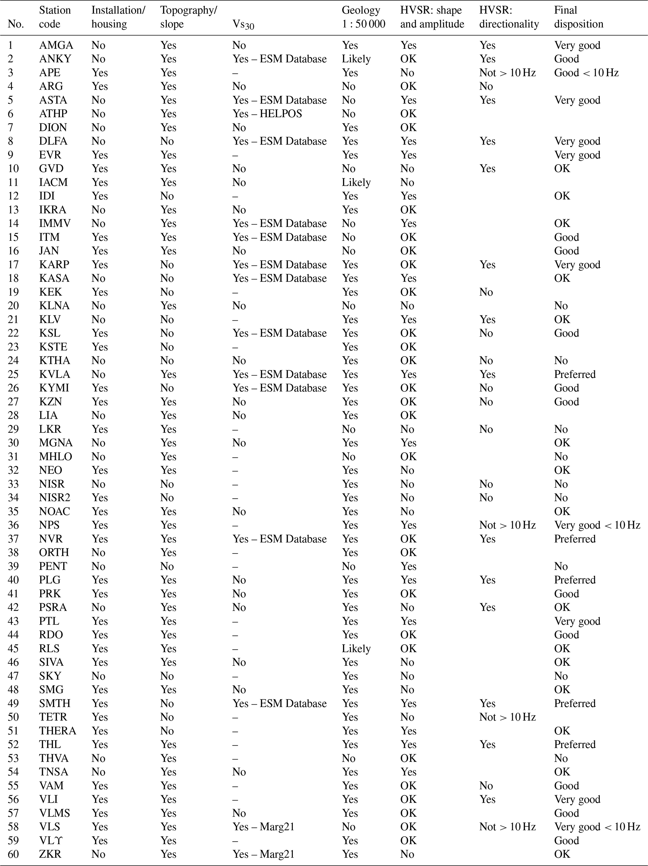
In the previous sections, we compiled several descriptors for our stations and derived amplification characteristics from our strong-motion data analysis. We bring everything together in Table 2 to co-evaluate the overall potential of our stations as reference stations. We take into account all criteria, challenging all parameters by openly contrasting them. We do not attribute numerical values and weights to each parameter, as is done e.g. in the summation rationale of Lanzano et al. (2021). We believe there are inherent problems with quantifying qualitative data and treating them as homogeneous in order to perform mathematical operations between them. Moreover, our goal is not to provide a continuous ranking across all sites. We opt for assessing all data together to offer an overall qualitative assessment of reference site potential. In Table 2 we regard stations that got a positive assessment in six factors as “preferred” reference sites (five instances). Those who missed one field are considered “very good” (nine instances), and those that missed two or three fields are classified as “good” or “OK”, noting bandwidth. Stations that ranked lower are not generally recommended, though the user can select them for specific purposes or within specific frequency bands according to their own judgement. Different schemes could be contrived to evaluate and even prioritise the stations, but we do not feel absolute grading is necessary. Besides, selection also depends on the specific application that uses the reference motion. It is an important message to convey that over half of the stations did not rank as reliable enough reference stations, and we feel that more work is needed to reassess the implications of this finding. Some of our rock sites also had high-frequency amplifications: this is in line with the definition of A-class sites in EC8, which is shifting from the current version (CEN, 2004) of Vs₃₀> 800 m s⁻¹ to a new version (Labbé and Paolucci, 2022) where there is also a provision for f₀>10 Hz.

In this study, we compute FAS-based HVSR for the first time for all the HL rock stations. This produces a rich suite of metadata that greatly exceeds the outcomes of typical HVSR analysis. We also compile parameters from various sources (housing/installation, topography/slope, surface geology, and Vs₃₀). We compare and contrast those metadata from various sources, and, in addition, we offer insights and corrections based on site visits from the network operator. We believe the operator's first-hand experience is very important because geological maps constructed at such a scale to serve an entire country (and made by different teams, over several decades) inevitably contain errors and simplifications, whereas a site walkover by an experienced geologist is more reliable. Similarly, satellite-based estimates of slope/topography invariably include approximation, homogenisation, and lack of specificity depending on the size of the pixel, whereas again a site visit leaves little doubt as to the exact nature of the landscape at the exact location of the station. The information for rock stations up to now has been sparse and scattered for the strong-motion sites and almost non-existent for the broadband sites. Until now, reference stations in the HL network could only have been selected based on a search of geology, or one may even have considered all rock stations to be interchangeable. We hope this work has provided a first step towards a better evaluation of rock stations and eventually towards better utilisation of their data. We believe this work is in line with user needs. For instance, Zhu et al. (2020) asked all networks to share not only station f₀ values, but also preferably their entire amplification functions. We think this study's outcomes exceed what has been asked because we enhance the typical HVSR method results in three ways (exhausting usable bandwidth, correcting for vertical, and investigating directionality). Moreover, by compiling literature-, map-, and operator-derived information, we offer the user transparency of all criteria and the possibility to prioritise and tailor them to individual needs. Until now, a user might likely select a reference station from the HL based on a single source of information, which would carry larger risks with respect to using our collation of parameters. We have shown that the selection process matters and that not all rock sites should be treated equally or trusted blindly.

Finally, we believe that data-derived transfer functions are extremely important for understanding station response. There is sometimes a fixation on Vs₃₀. Not only is this inadequate (too shallow and providing no indication of impedance depth or contrast), but also may even be unnecessary if we have both the geology and – what is more – the empirical site response from recordings. Even a full Vs profile may be inadequate to assess site response, considering that its high frequencies depend heavily on the assumptions made on damping and – most of all – that its premise is the 1D assumption, which in nature is rarely the case, especially for rock sites. On the other hand, empirical estimates of site effects may have their shortcomings but reflect the 3D nature of the formations. Our study has shown that not all rock sites should be treated equally. We also ask the following question: when in possession of a data-derived site response, how much importance should be given to stand-alone meta descriptors and proxies such as Vs₃₀?

Appendix A

Table A1 Detailed results of the HVSR analysis for the stations in this study. Bold characters indicate cases where a peak is identified in HVSR after VACF correction where there was none before.

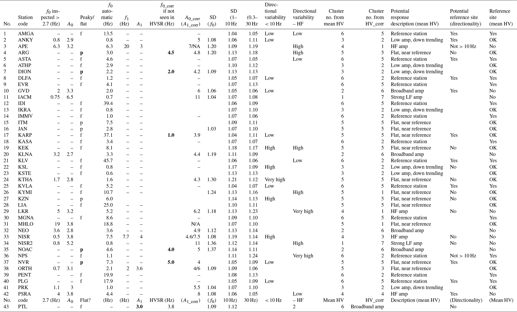
Table A2 Housing and installation conditions for the stations in this study.

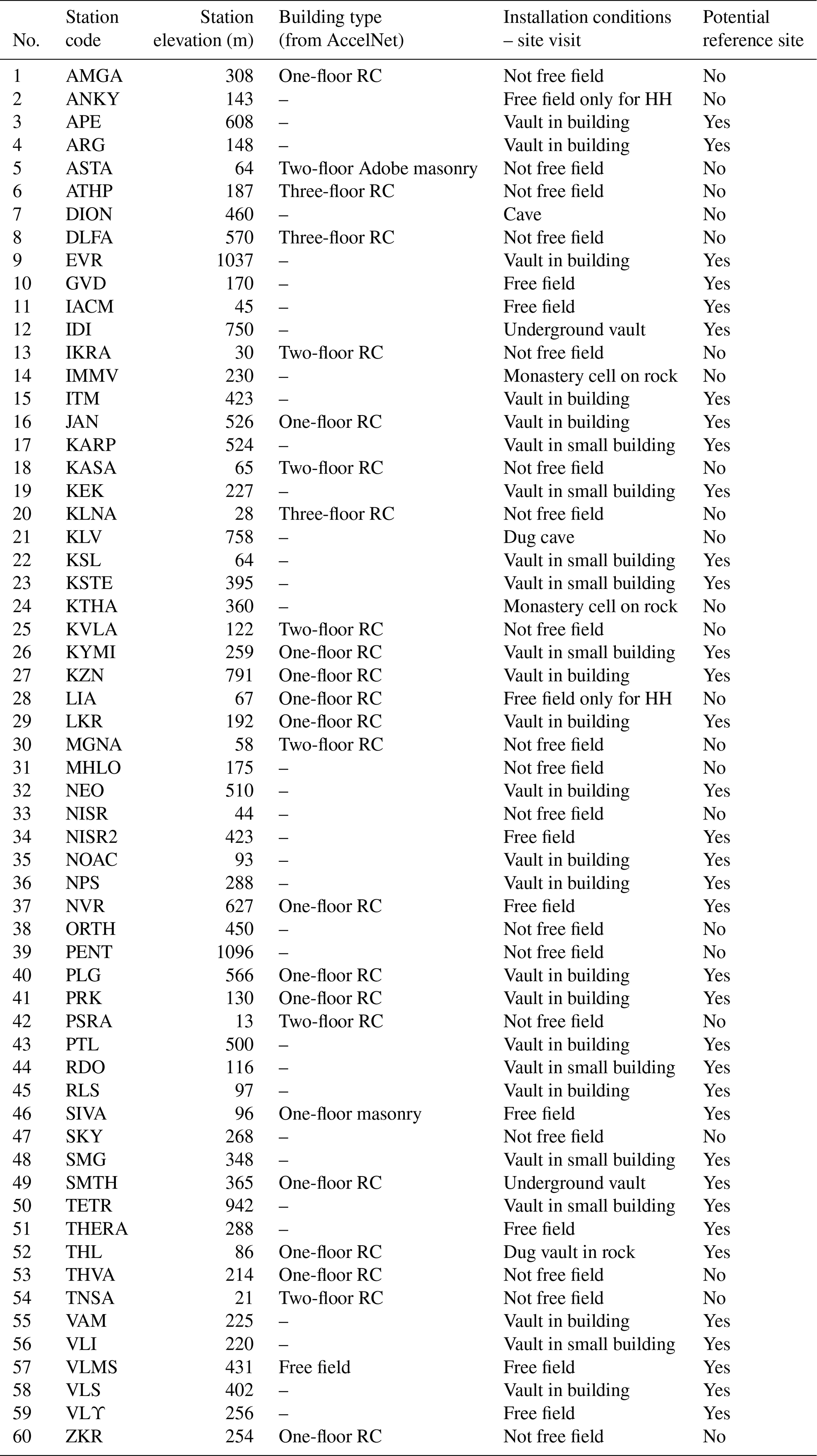
Table A3 Topography and slope conditions for the stations in this study. Bold italics indicate stations where the slope is non-negligible.

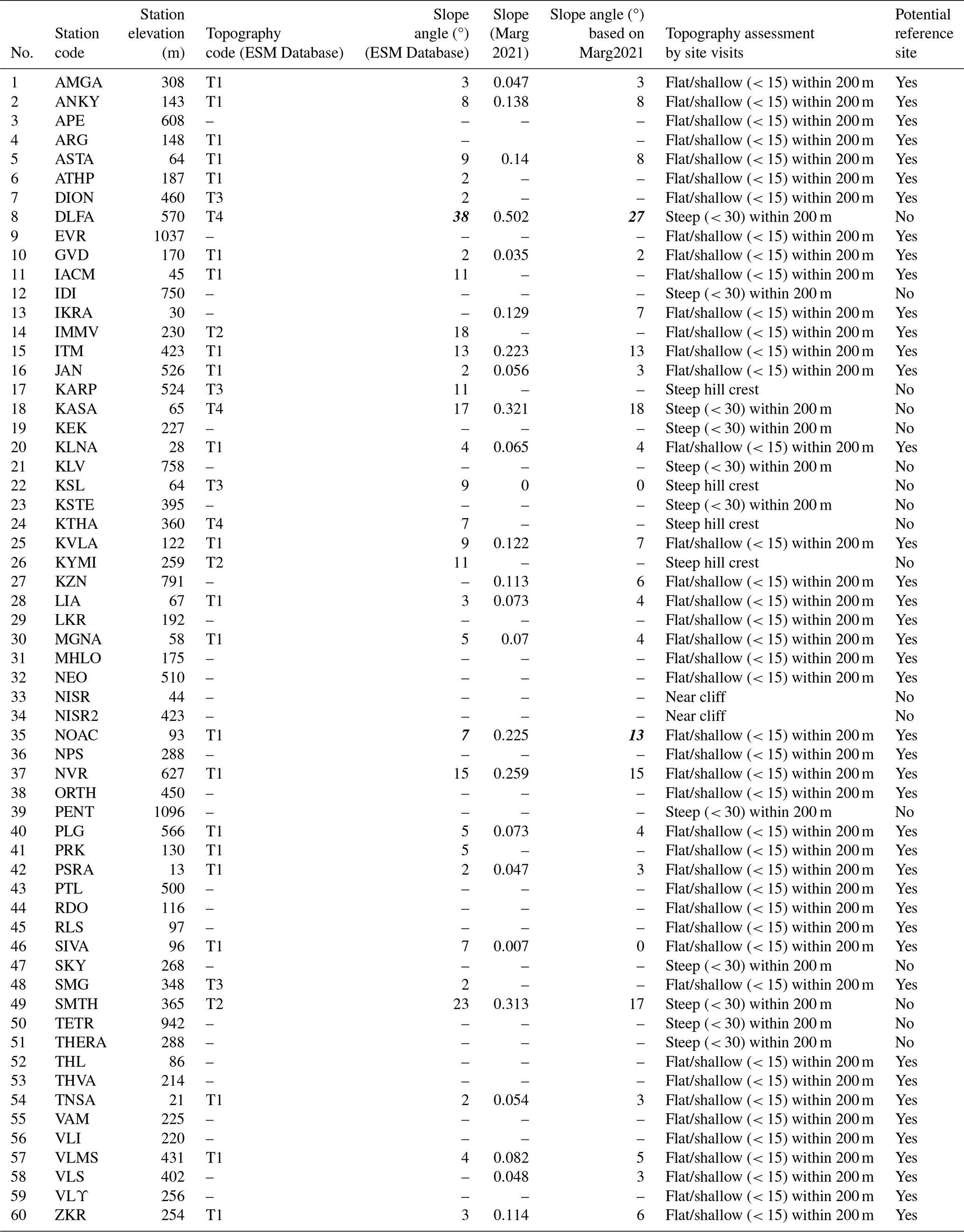
Table A4 Vs₃₀ estimates for the stations in this study. The strongest contradictions between sources leading to a jump in site class are marked in bold italics.

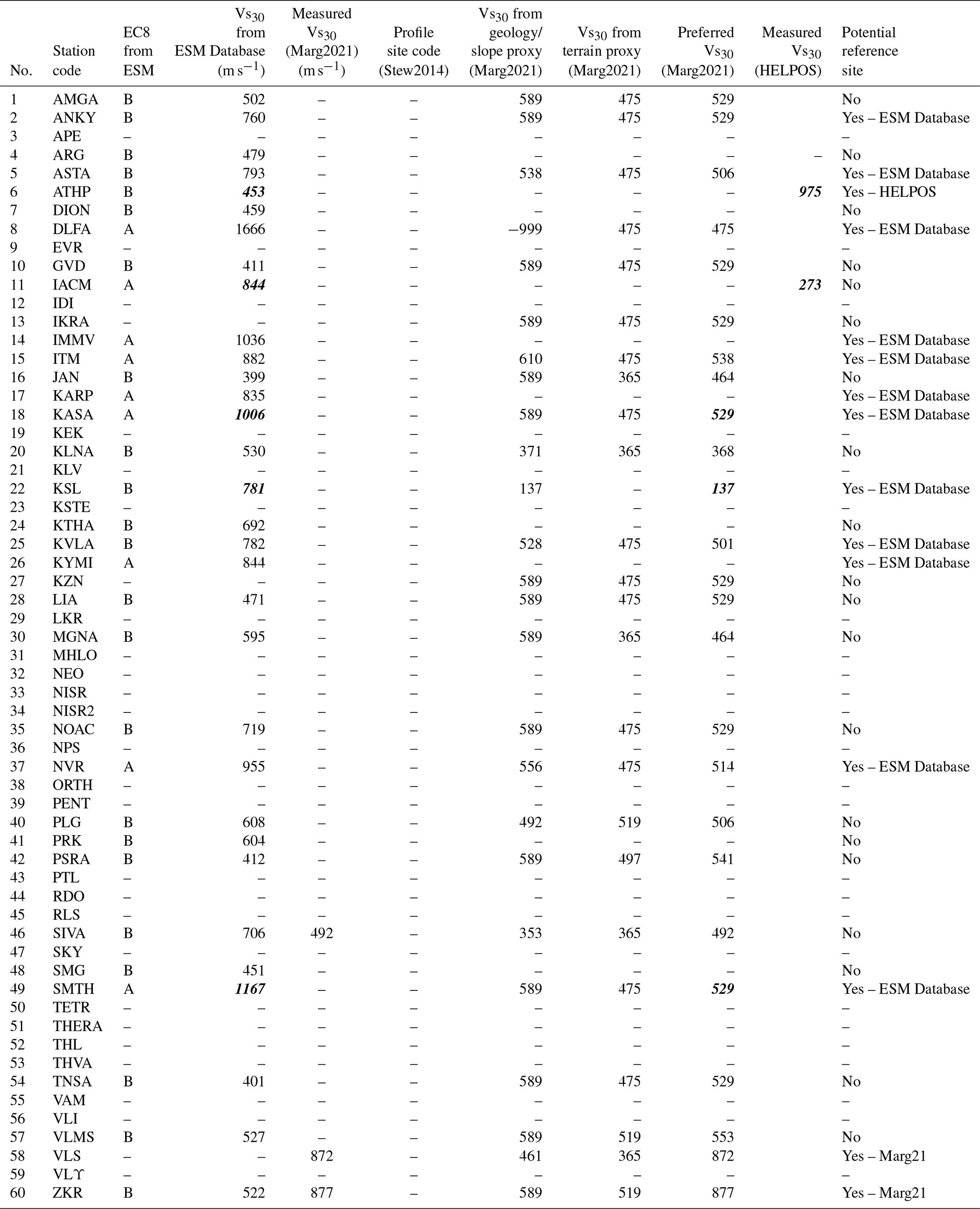
Table A5 Geological conditions including geological unit and age for the stations in this study.

Appendix B

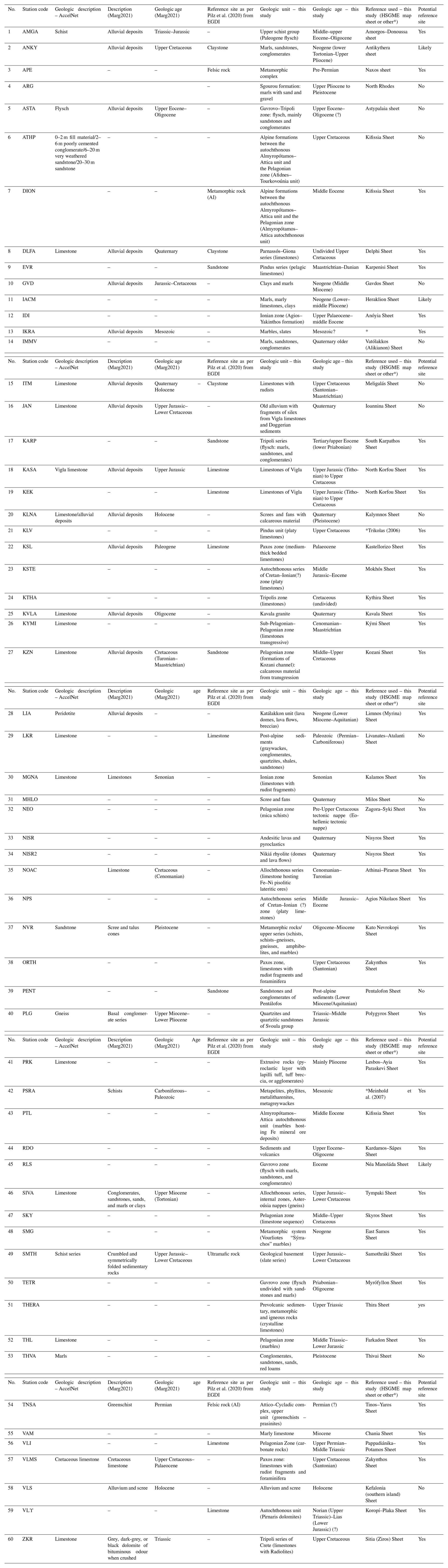
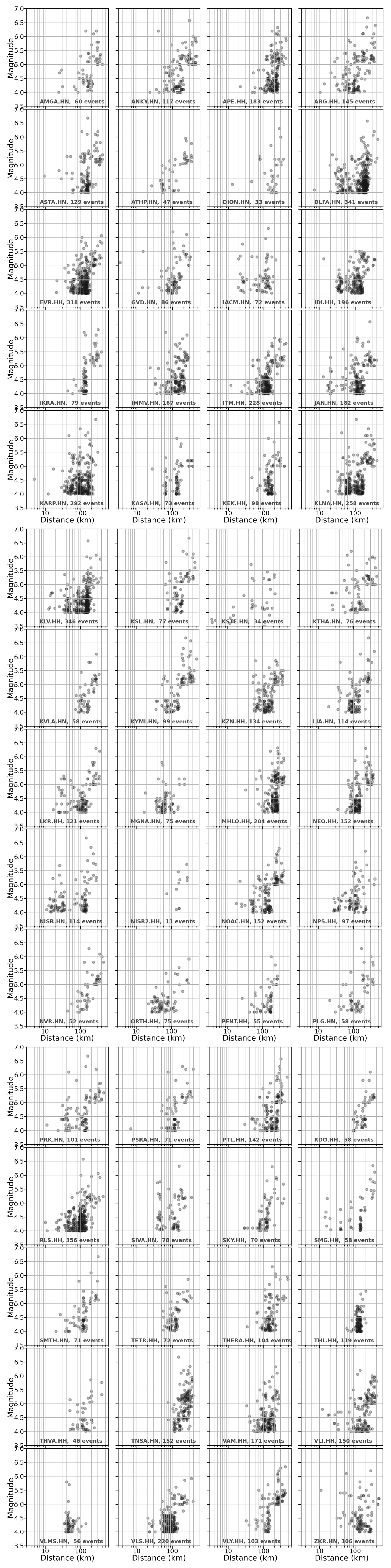
Figure B1 Distribution of magnitude (local) and distance (epicentral) for all data analysed per station. Fill colour indicates the density of recordings.

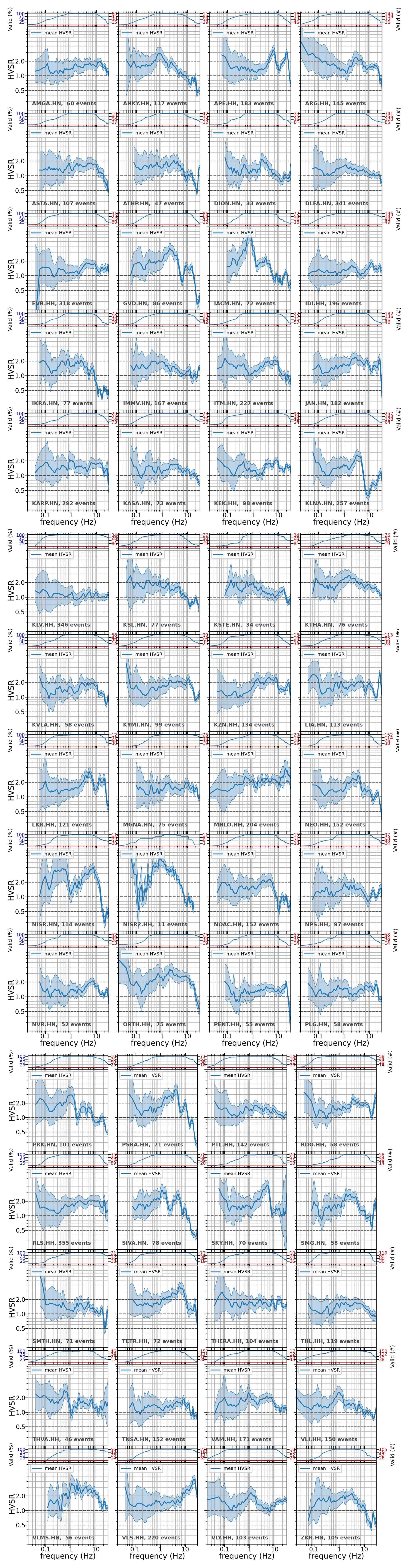
Figure B2 Mean orientation-invariant (SRSS) HVSR ± 1 standard deviation for all stations. Dashed horizontal lines indicate a factor of 2 from unity. Responses within this range would indicate passable behaviour for a reference site.

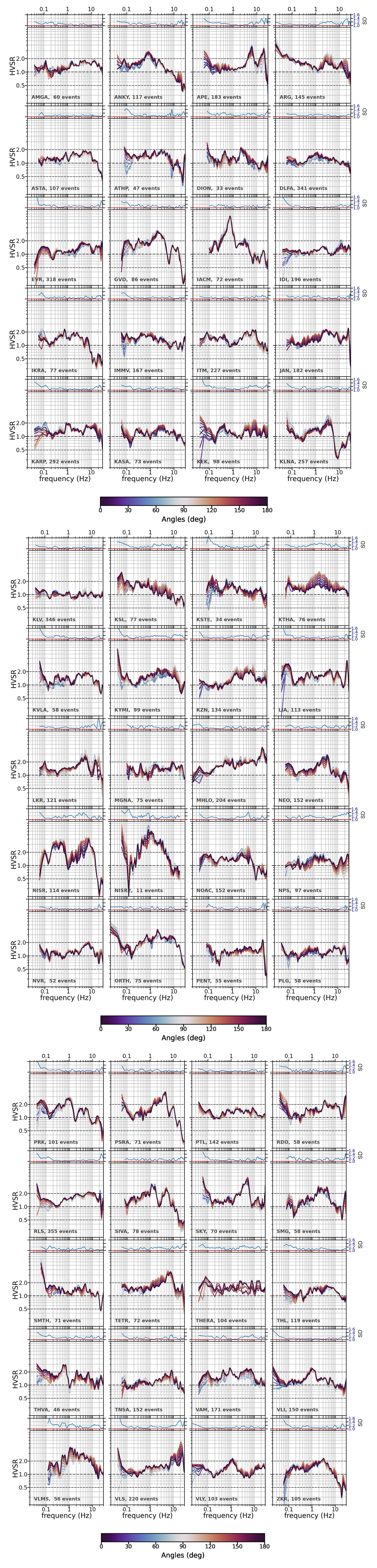
Figure B3 HVSRs per component, as those are rotated by 10° intervals from north to east for all stations. Dashed horizontal lines indicate a factor of 2 from unity.

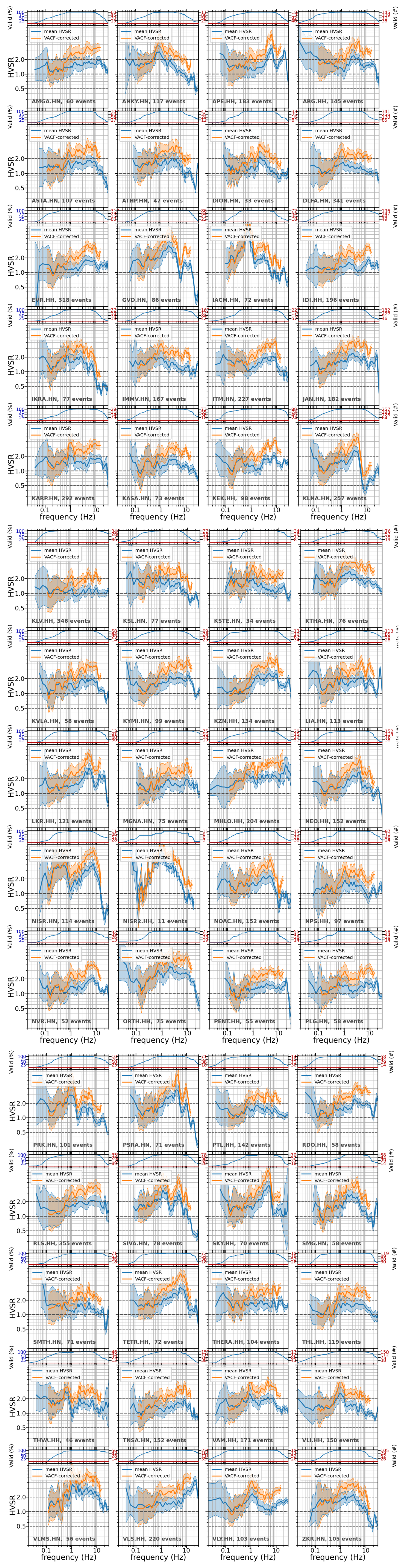
Figure B4 Mean orientation-invariant (SRSS) HVSR ± 1 standard deviation for all stations (in blue) and VACF-corrected HVSR using the Ito et al. (2020) vertical component correction function (in orange). The latter is only computed within the method's range of applicable frequencies and is offered in an indicative quality.

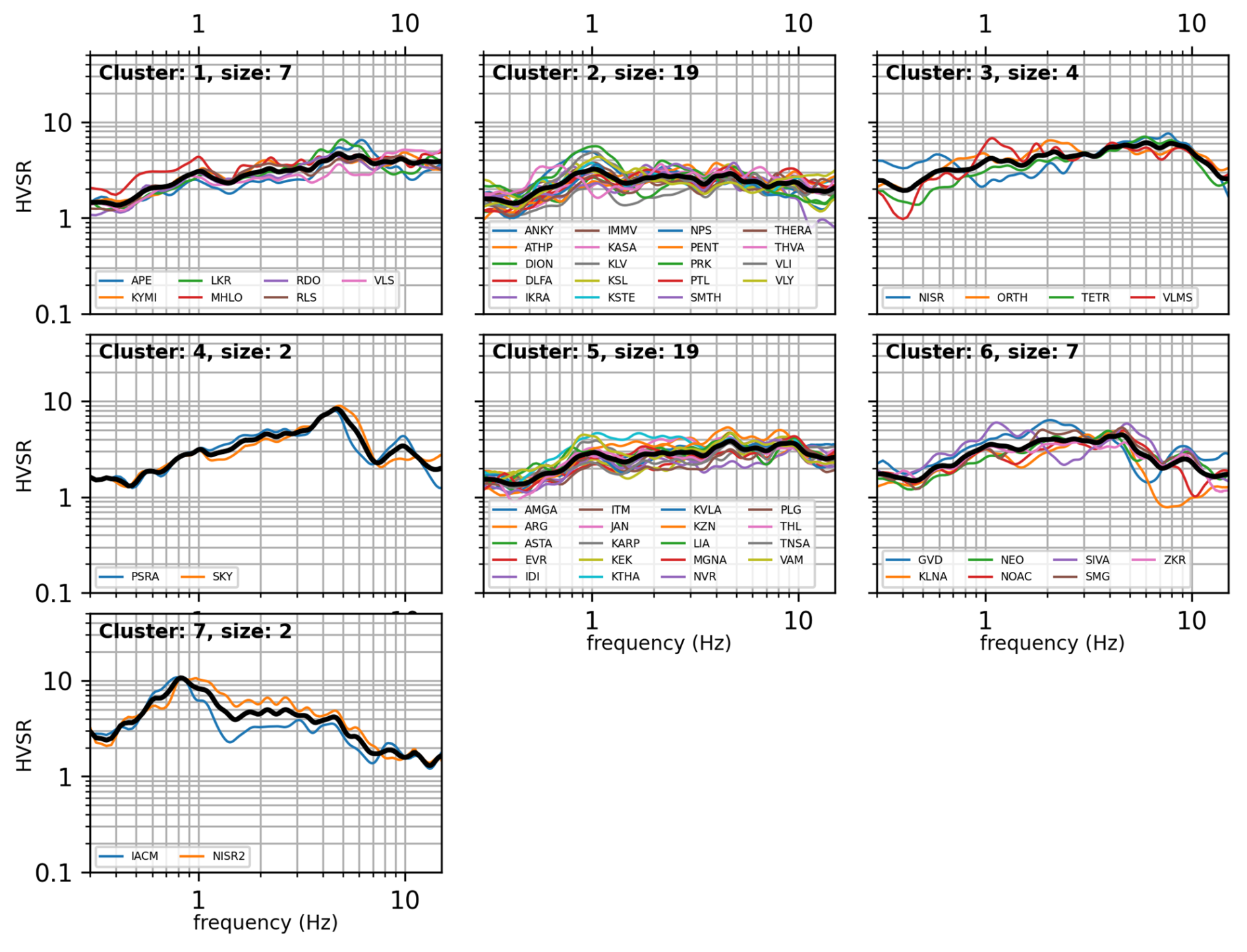
Figure B5 Groups of stations with similar amplification based on mean VACF-corrected HVSR, offered in an indicative quality.

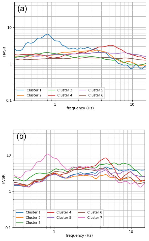
Figure B6 Clustering of stations based on (a) mean HVSR and (b) mean VACF-corrected HVSR, with the latter offered in an indicative quality.