Basin-scale geometric focusing: a probabilistic-geometric framework for global tsunami exposure assessment and the 2025 Kamchatka Peninsula tsunami

We present a hybrid probabilistic-geometric framework that integrates probabilistic earthquake statistics with large-scale ray-tracing simulations to efficiently map global coastal tsunami exposure. Utilizing a catalog of historical tsunamigenic events and the Gutenberg–Richter relation, we derive probabilistic weights for 9000 rays released across potential fault zones. The simulated ray pathways reveal persisting bathymetry-driven energy convergence patterns that govern far-field coastal focusing and shadowing. The geometric framework's predictive power is demonstrated using the 2025 M 8.8 Kamchatka Peninsula earthquake and the 2011 M 9.0 Tohoku-oki event. Validation against these events utilizes phase-corrected FUNWAVE-TVD simulations and in-situ DART observations. The resulting ray-based coastal focusing patterns display strong qualitative and quantitative spatial agreement (e.g., Spearman's ρ = 0.66 and ρ = 0.63, respectively) with the transoceanic maximum wave amplitudes from the high-fidelity FUNWAVE-TVD model. This agreement confirms the hybrid probabilistic-geometric approach as a scalable and computationally efficient tool for rapidly identifying transoceanic focusing potential and prioritizing coastal regions for high-resolution exposure assessment, mapping relative geometric convergence.

1 Introduction

Transoceanic tsunamis, typically generated by large-magnitude megathrust earthquakes in subduction zones, represent one of the most far-reaching and destructive natural hazards to coastal populations worldwide. As these long-wavelength waves traverse entire ocean basins, their energy does not disperse uniformly. Instead, the complex three-dimensional structure of ocean bathymetry, comprising mid-ocean ridges, fracture zones, seamount chains, continental shelves, and deep-ocean trenches, acts as an intricate system of refractive lenses. This bathymetry-driven refraction can channel, redirect, and sometimes trap tsunami rays, producing regions of pronounced geometric focusing. The resulting distribution of tsunami energy at landfall is highly heterogeneous: some coastlines, even thousands of kilometers from the source, experience severe and often unexpected wave amplification, while other areas may remain largely unaffected, forming classical shadow zones. This basin-scale sensitivity to bathymetric structure highlights the need for reliable tools capable of resolving the principal ray pathways that govern far-field tsunami exposure, especially given that these spatially variable pathways originate from the heterogeneous source distribution shown in Fig. 1a. While tsunamis can be triggered by non-seismic sources such as submarine landslides or volcanic eruptions, the vast majority of basin-wide events are generated by submarine earthquakes, which account for approximately 80 % of all recorded damaging tsunamis (Davies et al., 2018; Behrens et al., 2021). Non-seismic tsunamis, although potentially devastating in the near-field, typically involve more localized sources that produce shorter-wavelength waves. These waves are more susceptible to frequency dispersion, causing their energy to decay more rapidly with distance and limiting their far-field significance (Harbitz et al., 2014; Sannikova et al., 2021). For this reason, the present study focuses exclusively on the far-field propagation of seismically generated tsunamis. To specifically isolate the influence of ocean basin geometry, rays are intentionally released in the oceanward direction. Shoreward-directed waves are purposely excluded, as their propagation is predominantly governed by local near-source complexities rather than basin-scale topography. This directional constraint not only isolates the transoceanic focusing mechanics but also allows for the use of a coarser computational mesh optimized for deep water. Therefore, this framework is designed to guide decision-making for rapid, basin-scale transoceanic exposure assessment and to prioritize distant coastlines for computationally intensive nearshore modeling (run-up and inundation). Conversely, the method is explicitly not suitable for assessing non-seismic events due to their dispersive nature, leaving site-specific inundation mapping and local evacuation planning to specialized near-field hydrodynamic tools.

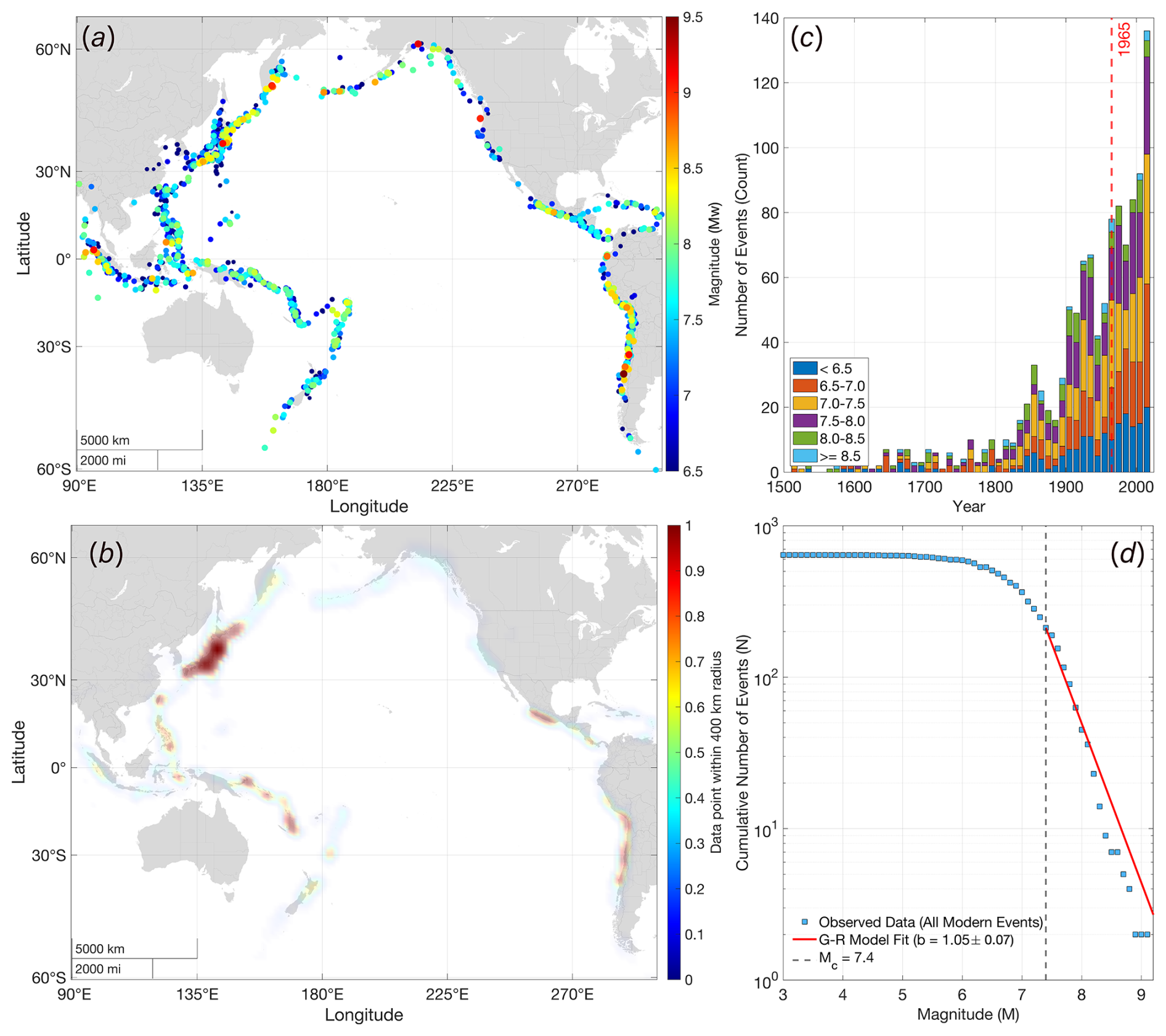
Figure 1 (a) Historical tsunamigenic earthquakes based on ∼ 1600 events from ∼ 500 BCE to 2025. The colormap indicates event magnitude (M_w); (b) spatial density plot (heatmap) showing earthquake clustering, calculated with a 400 km radius of influence; (c) histogram of historical events per decade since 1500, with bars color-coded by event magnitude. The vertical red line at 1965 marks the start of modern event records used in this study; (d) b-value estimate, showing the Gutenberg–Richter model fit (red line) to historical data since 1965 for events of magnitude ≥ 7.4. Basemap created with Natural Earth data.

Given the strong influence of bathymetric refraction on transoceanic tsunami propagation, evaluating basin-scale convergence traditionally relies on full numerical models, which become computationally prohibitive for large scenario ensembles. Alternatively, geometrical-optics methods (ray-tracing) capture dominant bathymetric refraction at a fraction of the computational cost. Foundational studies (Satake, 1988) demonstrated that tsunami rays accurately reconstruct principal pathways. More recently, Tehranirad et al. (2015) benchmarked ray-tracing against high-resolution dispersive models (FUNWAVE-TVD), finding strong spatial correlation between ray convergence and maximum surface elevations. Since seismically generated tsunamis are dominated by the non-dispersive shallow-water approximation over transoceanic distances, the ray-tracing method serves as a robust proxy for rapid scenario screening and global-scale seismic tsunami exposure assessment.

However, identifying the pathways of geometric focusing represents only one component of the broader exposure assessment problem. A realistic global exposure assessment must also reflect the inhomogeneous recurrence rates of tsunamigenic earthquakes across subduction systems. Early ray-based studies were inherently deterministic, typically initiated from a single, hypothetical earthquake source. Such simplified treatments do not capture the full range of seismic variability across global subduction systems and therefore cannot produce a comprehensive or realistic depiction of global tsunami exposure. Modern hazard assessments must confront two key challenges: (1) the probabilistic nature of earthquake occurrence across distributed and heterogeneous source zones, and (2) the computational scalability required to evaluate tens of thousands of plausible rupture scenarios. This latter requirement motivates the use of Probabilistic Tsunami Hazard Assessment (PTHA), a framework that quantifies risk by estimating the exceedance probabilities (or return periods) of tsunami intensities at specific locations. PTHA couples statistical models of earthquake recurrence, often based on the Gutenberg–Richter relation, with numerical or analytical models of tsunami generation and propagation. Comprehensive reviews such as Grezio et al. (2017) and global assessments like Davies et al. (2018) outline how PTHA can be applied at regional to global-scales by integrating multiple source zones to construct hazard curves and probability maps.

To address this methodological gap, we introduce a hybrid probabilistic geometric modeling framework that couples classical ray-tracing with earthquake probability statistics to produce a fast, scalable, and scientifically robust global exposure mapping tool. Our approach integrates Gutenberg–Richter-based frequency–magnitude relationships with large-ensemble ray-tracing simulations, enabling efficient evaluation of far-field tsunami exposure while retaining the essential bathymetric controls. In our implementation, 9000 rays are released from candidate fault segments worldwide, each ray assigned a probabilistic weight (representing the annual rate, λ) derived from local and regional seismicity rates. It is important to clarify that in this framework, λ serves strictly as a source weighting factor to modulate the relative density of the ray field; it does not represent a direct probability of coastal amplitude exceedance. This approach allows us to rapidly quantify coastal energy convergence and identify global tsunami hotspots most susceptible to long-range focusing, while providing a probabilistic interpretation of exposure consistent with modern hazard assessment standards.

This paper is organized as follows. Section 2 presents the Probabilistic Tsunami Exposure Assessment methodology. Historical seismological data are analyzed to map the spatial distribution of tsunamigenic sources and to estimate their return periods for earthquakes exceeding magnitude 7.4. Section 3 introduces the wave ray-tracing method, based on the principles of geometrical optics. This approach simulates tsunami propagation paths from the identified source regions, with the resulting ray patterns revealing how ocean basin geometry and bathymetric refraction generate zones of energy focusing and shadowing. These patterns provide a first-order assessment of regional tsunami exposure. Section 4 presents a validation case study of the M 8.8 Kamchatka Peninsula earthquake. It begins with a high-fidelity Boussinesq-type simulation using the FUNWAVE-TVD model, hereafter referred to as FUNWAVE, to compute tsunami wave amplitudes. Next, the ray-tracing model is applied to predict tsunami energy convergence zones (focal points) for the same event. The resulting numerical simulations are compared against in-situ observations to assess both the accuracy of the ray-tracing predictions of focal zones and the wave heights simulated by FUNWAVE. Section 5 extends this verification framework by applying the combined ray-tracing and hydrodynamic models to the 2011 M 9.0 Tohoku-oki tsunami as a secondary validation case. Finally, Sect. 6 summarizes the findings and provides concluding remarks.

2 Probabilistic Tsunami Exposure Assessment

To create a spatially variable weighting scheme for tsunami sources, a simplified recurrence-weighted exposure screening was conducted (Grezio et al., 2017). The process is based on deriving earthquake recurrence parameters from a historical catalog Geophysical Data Center/World Data Service(NGDC/WDS) (2024) of tsunamigenic events and applying these parameters to a set of discrete source points along known and potential earthquake zones. The final output is the mean annual rate of occurrence for earthquakes, which serves as a quantitative weight for the subsequent ray-tracing model.

The historical catalog comprises approximately 1600 global events. Figure 1a illustrates the spatial distribution of these events, where color indicates the magnitude of tsunamigenic earthquakes recorded from 500 BC to 2025. Panel (b) shows the occurrence rate, while panel (c) presents the decadal histogram color-coded by magnitude. The establishment of the World-Wide Standardized Seismograph Network (WWSSN) in 1965 is marked by a vertical red line.

2.1 Gutenberg–Richter Recurrence Relationship

The frequency-magnitude distribution of earthquakes is modeled by the Gutenberg–Richter (G-R) law:

$$\begin{array}{}\text{(1)}& {\log }_{\mathrm{10}}\left(N\right)=a-bM\end{array}$$

where N is the cumulative number of earthquakes with a magnitude greater than or equal to M. The parameter b describes the relative proportion of small to large earthquakes, while the a-value represents the overall seismic productivity of a region.

To determine a stable b value, the catalog was filtered to include only the modern instrumental period (1965 onward), corresponding to the establishment of the World-Wide Standardized Seismograph Network (WWSSN). The Magnitude of Completeness (M_c) was initially assessed using the Maximum Curvature (MAXC) method (Woessner, 2005), which defines the completeness threshold by identifying the maximum value of the first derivative of the frequency–magnitude curve. For this dataset, the raw MAXC peak occurs at M_w = 7.05. However, because raw MAXC estimates frequently fall within the catalog's detection roll-over region and can therefore underestimate true completeness, we adopted a conservative operational threshold of M_c = 7.4. We emphasize that this threshold represents a modeling choice to ensure absolute catalog completeness rather than an exact, immutable catalog property. To ensure robustness, we evaluated the stability of the estimated b value over nearby completeness thresholds (e.g., M_c = 7.3 to 7.5), confirming that the principal basin-scale recurrence patterns are not materially altered. Based on the resulting complete subset of 212 events, a b value of 1.05 ± 0.07 was calculated using the Aki–Utsu maximum likelihood estimator (Fig. 1d), where the standard error is given by σ_b = $b/\sqrt{N}$ (Aki, 1965; Utsu, 1965).

A Magnitude of Completeness (M_c) of 7.4 was mathematically determined using the Maximum Curvature (MAXC) method, identifying the point of maximum first derivative in the frequency-magnitude curve. Based on the resulting subset of 212 events, a b value of 1.05 ± 0.07 was calculated using the Aki–Utsu maximum likelihood estimator (Fig. 1d) (Aki, 1965; Utsu, 1965). This value is consistent with the global average (b = 1), indicating a robust fit (Frohlich and Davis, 1993).

2.2 Spatial Seismicity Rate Estimation

For the sake of applicability, a polygonal curve Γ(Lat, Long) was first defined to pass through the historical epicenters, representing both known and potential earthquake zones. The curve Γ was constructed by interpolating through the historical epicenters and aligning with major subduction interfaces and fault boundaries identified from global tectonic maps.

The continuous curve Γ was constructed by tracing the major tsunamigenic fault systems and subduction interfaces globally, discretizing this path into 10 km intervals. To account for the spatial scatter of historical earthquakes, epicenters located within a [400] km search radius were orthogonally projected onto the nearest segment of this curve before applying the 1D Gaussian smoothing.

To account for spatial variability in historical seismic occurrence (Fig. 1b), a spatially varying a(Γ) value was derived using one-dimensional Kernel Density Estimation (KDE) along the along-trench coordinate Γ. This approach mitigates data sparsity by smoothing the influence of historical events over their surrounding segments. A Gaussian kernel f(Γ) was applied at the projected 1D location (Γ_i) of each event:

$$\begin{array}{}\text{(2)}& f\left(\mathrm{\Gamma }\right)={\displaystyle \frac{\mathrm{1}}{\mathit{\sigma }\sqrt{\mathrm{2}\mathit{\pi }}}}{e}^{-\frac{{\left(\mathrm{\Gamma }-{\mathrm{\Gamma }}_i\right)}^{\mathrm{2}}}{\mathrm{2}{\mathit{\sigma }}^{\mathrm{2}}}}\end{array}$$

While near-field inundation modeling requires resolving complex 3D fault geometries, basin-scale transoceanic exposure screening is predominantly governed by macro-scale, along-trench variations in seismic productivity (Scourse et al., 2018). Therefore, this dimensional reduction to a 1D longitudinal projection is an established methodology for macro-scale hazard analysis (Scourse et al., 2018). A smoothing bandwidth of σ = 500 km was selected to satisfy established empirical scaling laws for subduction interface earthquakes. Because great megathrust events (M_w ≥ 8.5) are restricted by down-dip width saturation at approximately 200 km, their ruptures are forced to propagate longitudinally (Allen and Hayes, 2017). Established length-scaling relations indicate that the characteristic along-strike rupture length for M_w 8.8–9.0 earthquakes spans roughly 440–588 km (Blaser et al., 2010; Allen and Hayes, 2017). The 500 km KDE bandwidth therefore physically scales the probability density to match realistic rupture extents, eliminating the severe epicentral over-fitting that occurs with narrower bandwidths. A quantitative statistical evaluation (Fig. A1) confirmed that spatial variance stabilizes at this 500 km threshold, while the macro-scale spatial clustering remains stable and independent of the selected bandwidth (r > 0.95). This curve was subsequently normalized to match the total observed annual rate of events above M_c from the modern catalog, so that local variations do not inflate regional seismic productivity, producing an absolute annual rate density for each source point.

The final weight assigned to each source point i is its total annual rate of significant tsunamigenic earthquakes (M ≥ 7.4), calculated by applying the spatially determined a(Γ) from the KDE to the Gutenberg–Richter relationship and integrating over the relevant magnitude bins. This yields a single representative annual rate, λ, which serves as the input likelihood for the tsunami ray-tracing models. The corresponding exposure map, showing the average return period T = $\mathrm{1}/\mathit{\lambda }$, is presented in Fig. 2.

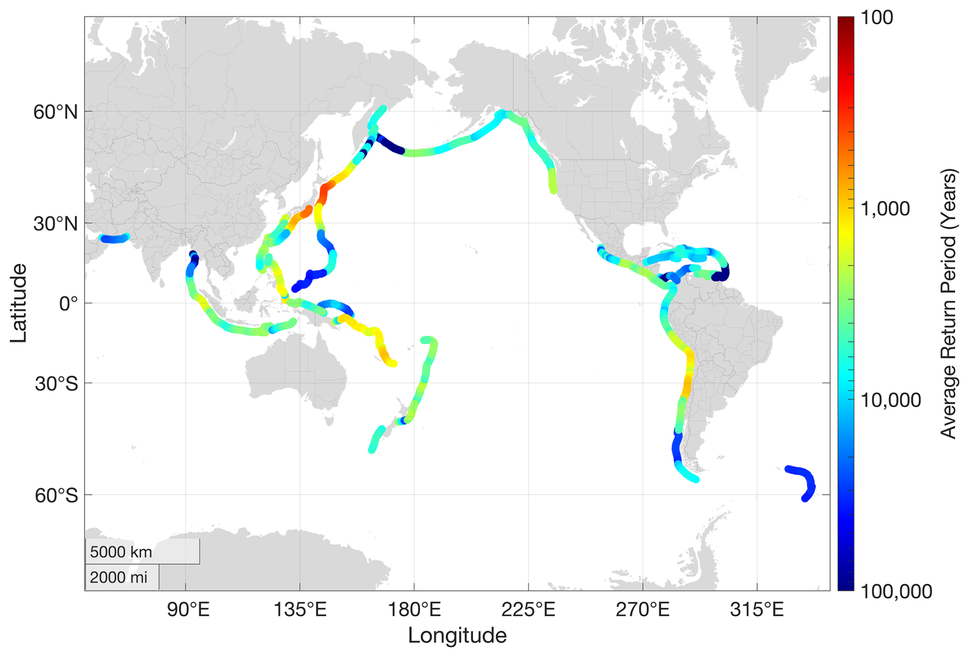
Figure 2 Return period of tsunamigenic earthquakes (M > 7.4) along the potential faults, based on historical data analysis, with a spatial resolution of 25 km. Basemap created with Natural Earth data.

The resulting exposure map reveals significant spatial heterogeneity in earthquake recurrence. The Kuril–Kamchatka and Japan Trenches in the northwest Pacific, alongside the Peru–Chile Trench in the southeast, emerge as the most seismically active source zones, exhibiting return periods between 100 and 1000 years (red to orange segments). This creates a dominant “exposure dipole” across the Pacific Basin. Additionally, the Aleutian Trench and the Sumatra–Andaman subduction zone show high recurrence rates, highlighting them as critical sources for transoceanic tsunami generation. In contrast, mid-ocean ridges and transform boundaries generally exhibit longer return periods (blue segments), reflecting their lower potential for generating large tsunamigenic displacements.

In this study we adopt a recurrence-based weighting, though we also examined whether magnitude-energy formulation would alter the resulting coastal exposure patterns. Using the same magnitude bins between M = 6.5 and 9.5, we computed an annualized energy metric Λ_j for each segment j by multiplying each bin's rate by E(M)∝10^1.5M and summing across bins. However, since the PTHA implementation employs a single regional b value and the same magnitude range for all source segments, the Gutenberg–Richter distribution has an identical shape everywhere. Under these assumptions Λ_j reduces to a constant multiple of the recurrence rate (Λ_j = Cλ_j), and thus energy-weighted ray-density field would be indistinguishable from the recurrence-weighted field up to a uniform rescaling. For this reason we present the recurrence-based maps, explicitly.

3 Ray-tracing Methodology

To simulate global tsunami propagation and identify regions of energy focusing or shadow zones, we use a numerical wave ray-tracing model based on the geometrical optics approximation. This approach tracks the trajectory of wave energy packets (rays) by solving a set of coupled ordinary differential equations (ODEs) over time. The theoretical framework follows standard formulations for surface gravity waves propagating over variable bathymetry and currents (Halsne et al., 2023).

3.1 Governing Equations

The model employs a kinematic ray-tracing approach. Rather than solving the dynamic transport equation for wave amplitude, which is prone to caustic singularities over complex deep-ocean bathymetry, we strictly solve the kinematic equations to track the trajectories of discrete wave energy packets. The state of a wave ray is defined by its position vector, x = (x,y), and wave number vector, k = (k_x,k_y). Their evolution in time t is governed by:

$$\begin{array}{}\text{(3)}& {\displaystyle \frac{\mathrm{d}\mathit{x}}{\mathrm{d}t}}={\mathit{c}}_{\mathit{g}}+\mathit{U}\text{(4)}& {\displaystyle \frac{\mathrm{d}\mathit{k}}{\mathrm{d}t}}=-{\mathrm{\nabla }}_h\mathit{\omega }-\left(\mathit{k}\cdot {\mathrm{\nabla }}_h\right)\mathit{U}\end{array}$$

Here, U = (U,V) is the ambient current velocity vector, c_g is the intrinsic group velocity vector, and ω is the intrinsic angular frequency of the wave. For far-field tsunami applications, ambient currents are negligible compared to the wave speed, so we set U = 0 in Eqs. (3)–(4). The angular frequency ω is related to the wave number magnitude k = $\left|\mathit{k}\right|=\sqrt{k_x^{\mathrm{2}}+k_y^{\mathrm{2}}}$ and local water depth d through the linear dispersion relation:

$$\begin{array}{}\text{(5)}& {\mathit{\omega }}^{\mathrm{2}}=gk\tanh \left(kd\right)\end{array}$$

Wave refraction is governed by the term −∇_hω in Eq. (4) (where U = 0). For the characteristic period spectrum evaluated in this study, the waves strictly satisfy the shallow-water limit even in the deepest oceanic trenches. Because the phase speed remains overwhelmingly depth-dependent, the bathymetric refraction gradients that dictate the ray trajectories are fundamentally unaffected by frequency dispersion. Since ω depends on both k and d, its horizontal gradient is primarily driven by bathymetric variations:

$$\begin{array}{}\text{(6)}& {\mathrm{\nabla }}_h\mathit{\omega }={\displaystyle \frac{\partial \mathit{\omega }}{\partial d}}{\mathrm{\nabla }}_{h}d\end{array}$$

and because no diffraction term is included here, rays cannot reproduce energy leakage around obstacles. This shows that changes in the wave number vector, and thus the propagation direction, are directly proportional to the local sea-floor gradient, ∇_hd, which is the main mechanism for tsunami refraction across ocean basins.

3.2 Numerical Implementation

The system of ODEs (Eqs. 3 and 4) is solved numerically to trace each ray's trajectory using a fourth-order Runge–Kutta scheme. Rays propagate over a global, unstructured triangular mesh comprising 1 726 063 nodes and 3 452 122 elements, with spatial resolution varying from 10.77 to 28.35 km (Fig. A2). The variable-resolution unstructured mesh is generated based on the shallow-water wave, ensuring that tsunami wavelengths are adequately resolved. During the mesh generation process, bathymetric gradients and all relevant geometric features that affect the wave refraction under study are explicitly taken into account. This feature-tracking preserves the steep bathymetric gradients necessary for accurate refraction, forcing finer nodal placement (down to 10.77 km) along critical structures like seamount peaks and trench fracture lines, while allowing coarser resolutions (up to 28.35 km) in relatively flat abyssal plains, without requiring a uniform, ultra-high resolution domain.

Bathymetric data are sourced from 2025 General Bathymetric Chart of the Oceans dataset (GEBCO Bathymetric Compilation Group 2025, 2025) with 15 arcsec resolution. Using a time step of 180 s and Courant–Friedrichs–Lewy CFL < 1, the depth-dependent resolution is set as the product of the time step and local group velocity, ensuring that no ray travels more than one element per time step. At each time step, environmental parameters are evaluated dynamically, as rays can lie anywhere within a mesh element. Water depth at a ray's latitude–longitude location is computed using barycentric interpolation from the nodal values of the containing element. The bathymetric gradient, ∇_hd, which drives wave refraction, is precomputed for all elements to improve computational efficiency.

3.3 Numerical Simulations

Rays are initialized along potential tsunami-generating fault lines, shown in Fig. 2, at 25 km intervals. To ensure comprehensive coverage of potential refractive pathways, rays are initialized across a discrete spectrum of characteristic tsunami periods spanning the typical empirical range of 15 min to 3 h at each source location. By aggregating this discrete period spectrum globally, the kinematic model effectively bounds the frequency-dependent variations in transoceanic energy focusing to construct the final exposure footprint. While real near-field radiation directivity depends on detailed 3D rupture kinematics – such as variable slip distribution, rake, and dip, the dominant macro-scale energy flux of large subduction megathrust earthquakes radiates predominantly orthogonal to the fault strike. Therefore, the initial propagation direction for all rays is set perpendicular to the local fault segment. This simplification natively encodes the primary radiation lobes required for transoceanic far-field propagation without necessitating complex 3D volumetric initializations. Furthermore, rays are oriented exclusively oceanward; shoreward-directed waves are excluded because their propagation is governed by local near-source complexities and non-linear shoaling, which fall outside the scope of basin-scale transoceanic exposure screening.

A ray is terminated if it reaches land (where water depth becomes zero or negative) or enters a user-defined shallow coastal zone (500 m depth). This cutoff is imposed to exclude the complex nearshore region where nonlinear shoaling dominates and where strong refraction often leads to ray crossing (caustics), rendering the standard geometrical optics approximation insufficient. Furthermore, as waves enter these shallower depths, their decreasing group velocities and shorter wavelengths would require a proportionally higher-resolution mesh. Implementing such fine resolution along global coastlines would impose prohibitive computational costs, directly defeating the primary utility of this framework as a rapid transoceanic exposure screening tool. In total, 9000 rays were released, and the simulation was run for 24 h, sufficient for all rays to reach a termination criterion. Upon termination, the spatial density of ray impacts along the coastline is calculated. By utilizing a ray-density proxy rather than a classical ray-tube energy flux calculation, the model natively bypasses the mathematical singularities associated with deep-water caustics (ray crossings). In this kinematic framework, caustics simply and stably register as localized zones of high ray concentration. This normalized ray termination count (ranging from 0 to 1) serves as a proxy for the relative probability of exposure (focusing potential), rather than a measure of dynamic wave amplitude or absolute energy flux, effectively mapping regions of energy convergence (focusing) and divergence (shadowing). This framework allows efficient and accurate simulation of tsunami propagation across complex global bathymetry, illustrating how basin geometry controls wave energy distribution. The simulations were performed on a 32-core Mac Studio with 512 GB of unified memory. The code is parallelized, and since each ray is treated independently, the 24-hour simulation completed in approximately 12 h. This ray-tracing approach captures tsunami exposure primarily for transoceanic propagation from the source across the basin to distant locations. Hazards in the immediate vicinity of the earthquake are not considered in this study, as our focus is on the effects of ocean-basin geometry on tsunami travel; near-source tsunamis may indeed be more catastrophic, but they fall outside the scope of this work.

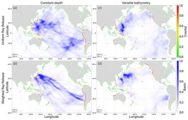
To systematically examine how source geometry, recurrence intervals, and bathymetric refraction shape global tsunami exposure, we designed four targeted numerical experiments. Each scenario isolates a fundamental driver of tsunami propagation: (i) fault geometry, which controls the initial azimuth and directional bias of energy release; (ii) variable bathymetry, which refracts and redirects wave trajectories across the basin; and (iii) probabilistic weighting, which modulates exposure intensity based on earthquake return periods. Figure 3 summarizes the outcomes, where basin-scale ray density is shown using a white-to-blue scale, and coastal focusing is highlighted by a green–yellow–red scale. All results are normalized by the global maximum to enable direct comparison across experiments.

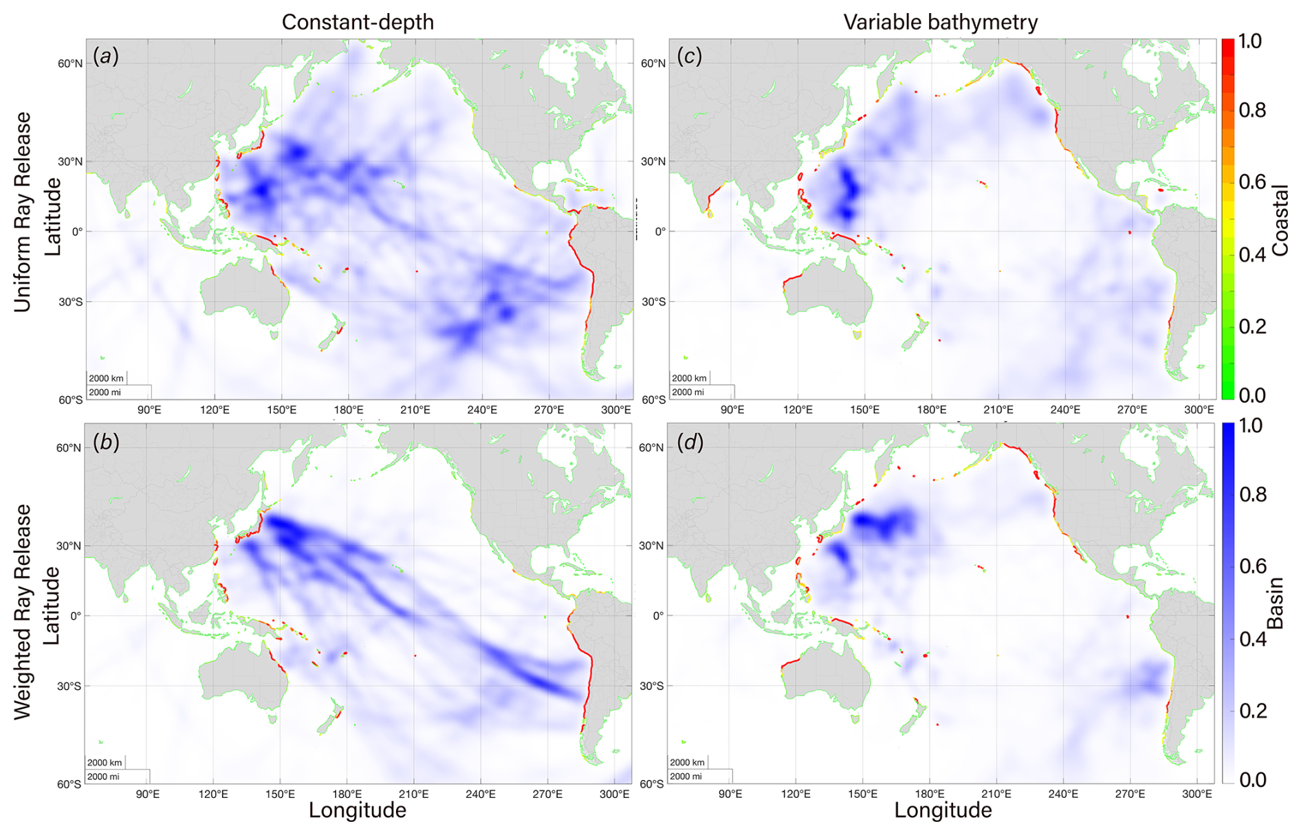
Figure 3 Basin-wide ray density and coastal tsunami exposure for 9000 tsunami rays released along potential fault zones (shown in Fig. 2). Panels (a) and (b) represent constant-depth cases, highlighting the effects of fault location and orientation, while panels (c) and (d) incorporate variable bathymetry to show the combined influence of seafloor geometry and fault configuration. The top row shows uniformly released rays, and the bottom row applies probabilistic weighting (using the annual rate parameter λ from Sect. 2) based on return period derived from the Gutenberg–Richter relation. The ocean-floor heatmap (white to blue) illustrates ray convergence and geometric focusing, and coastline colors (green–yellow–red) indicate relative coastal exposure using a normalized ray-count proxy (0–1), with redder areas denoting higher exposure. Basemap created with Natural Earth data.

Figure 3a–b adopt a constant-depth approximation, forcing rays to follow great circle paths (GC) and, by design, removing any effect of bathymetric refraction. This configuration exposes the sole influence of fault geometry and position, effectively reducing the ocean basin to a two-dimensional line-of-sight system. Under these conditions, a highly energetic corridor extends across the Pacific Basin, originating from the Kuril–Kamchatka and Japan trenches. This direct projection leads to a broad signature of exposure, producing normalized coastal exposure indices between 0.8 and 1.0 along the northeast coast of Australia, Papua New Guinea, and the Solomon Islands, as well as along South America. Panel (a), using uniform ray release, overemphasizes the role of smaller fault systems; panel (b) incorporates the probabilistic weights (λ) from Sect. 2, refining the magnitude but retaining the linear propagation patterns inherent to the constant-depth assumption, keeping exposure indices artificially high (∼ 0.8–1.0) along these direct line-of-sight coastlines.

In Fig. 3c–d, where realistic bathymetry is introduced, refraction and scattering fundamentally reorganize the tsunami wave-field. For example, the exposure corridor toward Northeast Australia is reduced by approximately 80 % (dropping from an exposure index of 0.8–1.0 down to 0.1–0.2) as rays encounter the complex topography of the Southwest Pacific – namely the Melanesian Arc and the Solomon Rise. In contrast, topographic structures in the North Pacific, such as the Emperor Seamount Chain and the Mendocino Fracture Zone, act as waveguides, channeling energy toward North America, increasing normalized coastal focusing in the Pacific Northwest by over 50 % (elevating the index from diffuse values of 0.4–0.6 up to highly localized peaks of 0.9–1.0) relative to the uniform depth case.

Panel (d) represents the most complete exposure characterization, combining realistic bathymetry with the probabilistic source weighting (λ). By modulating the intensity of each ray based on its source's annual occurrence rate, this configuration filters out low-probability contributions seen in panel (c). Notably, it reveals a reciprocal focusing pathway between South America and East Asia: the Kuril–Kamchatka system preferentially feeds energy toward Chile (index > 0.8), and the Peru–Chile trench returns a concentrated ray field toward Japan and the Philippines. Additionally, the model identifies a pronounced shadow zone in the Southeast Pacific – west of the East Pacific Rise – where ambient basin ray densities of 0.3–0.4 (seen in panel b) are reduced to near zero (< 0.05). Finally, the probabilistic approach intensifies the signal over the Bay of Bengal and the Indonesian archipelago, elevating the normalized exposure index from background levels (∼ 0.3–0.5 in panel c) to peak values exceeding 0.8, where high recurrence rates of tsunamigenic earthquakes lead to elevated exposure levels.

4 M 8.8 Kamchatka Peninsula event

On 29 July 2025, at 23:24 UTC, a moment magnitude (M_w) 8.8 earthquake struck off the eastern coast of Russia's Kamchatka Peninsula. The epicenter was located at 52.51° N, 160.32° E, approximately 136 km east-southeast of Petropavlovsk–Kamchatsky, at a depth of 35 km, according to the United States Geological Survey (USGS). The earthquake resulted from thrust faulting along the Kuril-Kamchatka subduction zone, where the Pacific plate subducts beneath the North American (Okhotsk) plate. This event ranks among the largest earthquakes globally since 2011 and is one of the six largest recorded in the modern instrumental era. The earthquake generated a trans-Pacific tsunami, with maximum run-up heights of about 3 m in Severo-Kurilsk, Russia, and up to 1.2 m in Hawaii (Geophysical Data Center/World Data Service(NGDC/WDS), 2024; NOAA, 2025a). While initial warnings indicated potentially higher impacts, the remote location and rapid alert system limited casualties and damage. One indirect fatality was reported in Japan, and several injuries occurred. In Kamchatka Krai, moderate damage was observed, including power outages and structural impacts in Petropavlovsk-Kamchatsky (Geophysical Data Center/World Data Service(NGDC/WDS), 2024; NOAA, 2025b; USGS, 2025). This event underscores the potential of large subduction zone earthquakes in the North Pacific to generate widespread trans-oceanic tsunami hazards and highlights the importance of early warning systems for coastal risk mitigation.

The initial condition for the tsunami propagation model FUNWAVE is the residual vertical seafloor displacement field generated using the elastic half-space model of Okada (1985). For the M 8.8 Kamchatka Peninsula event, this study utilizes two distinct source models, hereinafter referred to as the NOAA and USGS scenarios. The NOAA scenario is not derived from direct seismic measurements, but from an inversion of tsunami observations recorded at DART buoys. This approach uses the Method of Splitting Tsunami (MOST) model, which involves matching real-time observations to a linear combination of pre-computed tsunami waveforms from unit sources (Titov et al., 2005). The resulting source model for this event consists of nine sub-faults, with characteristics shown in Table 1. In contrast, the USGS scenario is based on seismological inversion using ground motion data and finite-fault analysis, resulting in a more complex source defined by 345 sub-faults (Hayes, 2017). The NOAA solution commonly performs better for tsunami propagation because it assimilates offshore DART waveforms. The vertical coseismic displacement fields for both scenarios are illustrated in Fig. 4.

Table 1 Fault parameters for NOAA scenario, with length 100 km, width 50 km, and rake 90°.

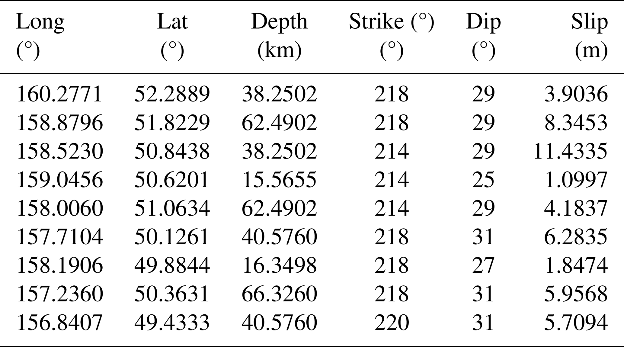
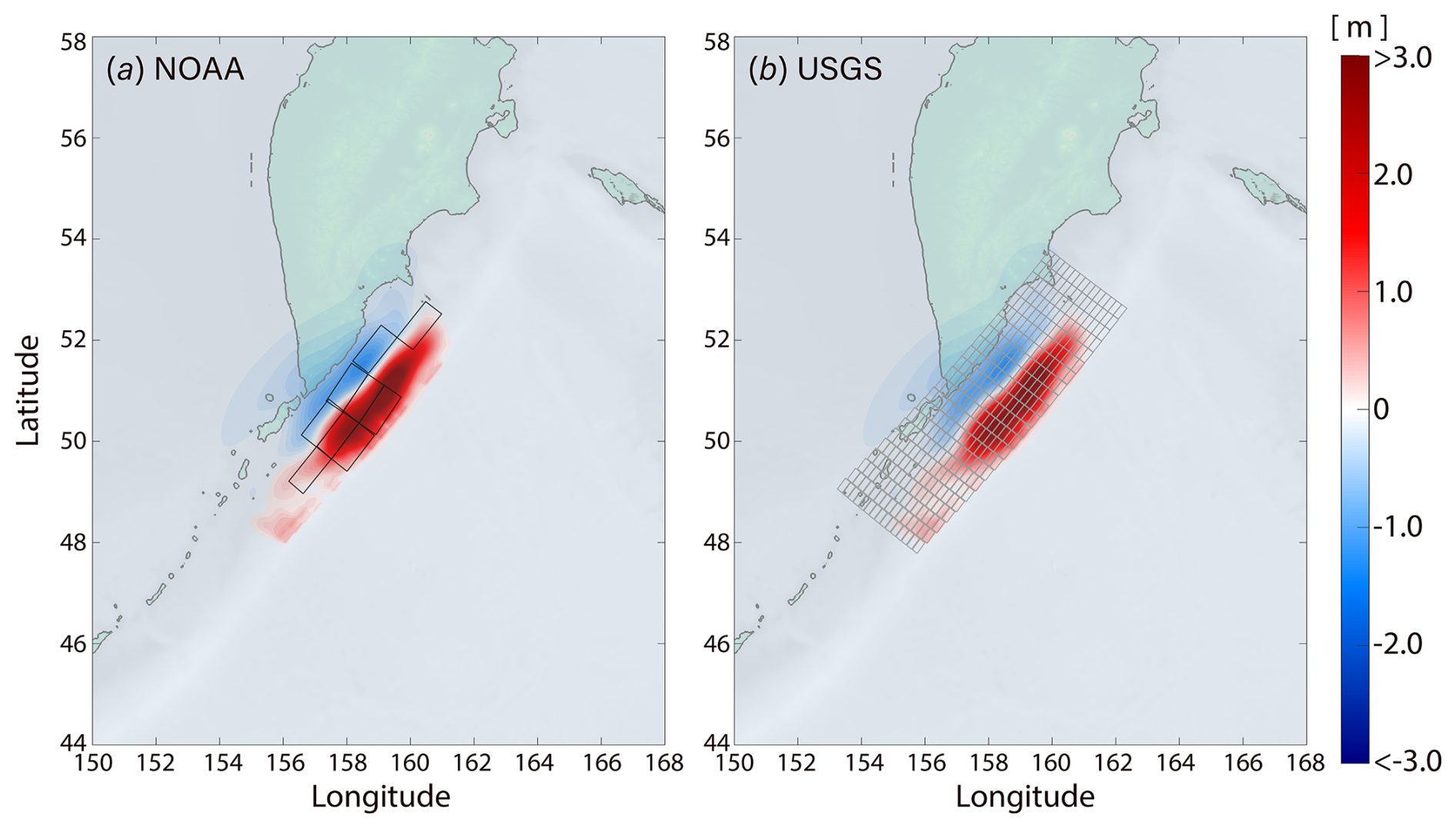
Figure 4 Residual vertical component of bed deformation for two scenarios based on inversion performed by (a) NOAA with 9 sub-faults with 50 × 100 km dimension and (b) USGS with 345 sub-faults with 15 × 30 km dimension.

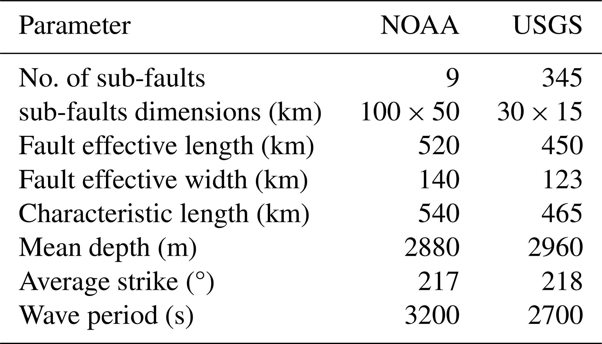
To quantitatively compare these sources and estimate key tsunami parameters, a standardized method is applied to each deformation field. First, the primary generation area is identified by a polygon enclosing all points where the absolute displacement exceeds a 10 % threshold of the maximum deformation. An oriented bounding box is then fitted to this polygon, yielding the source's effective length (L_eff), effective width (W_eff), and average strike. Subsequently, a single characteristic length (L_c) is derived as the hypotenuse of the effective dimensions (L_c = $\sqrt{L_{\mathrm{eff}}^{\mathrm{2}}+W_{\mathrm{eff}}^{\mathrm{2}}}$). This geometric proxy serves as a robust estimate for the dominant initial wavelength, explicitly linking the spatial extent of the seafloor uplift to the frequency content of the generated wave. This characteristic length, combined with the average ocean depth across the source region, is then applied to the linear dispersion relation to calculate the tsunami's characteristic wave period (Satake, 2005). Table 2 summarizes these effective fault and tsunami parameters for both scenarios. For validation, these model-derived periods are later compared against the wave period determined from an analysis of the observed DART buoy recordings for this event.

Table 2 Comparison of NOAA and USGS fault scenarios.

4.1 High fidelity modeling (FUNWAVE)

For the simulation of tsunami wave propagation, we use the Boussinesq-type wave model, FUNWAVE, in spherical coordinates (Kirby et al., 2013). The model has been validated against a large set of analytical, laboratory, and field benchmarks as part of the development of tsunami hazard maps for the US East Coast (Tehranirad et al., 2011). An optimized MPI parallel implementation of FUNWAVE was developed, which has highly scalable algorithms, with a typical parallel scaling efficiency of more than 90 % of the number of cores in a typical medium-sized computer cluster. This makes it possible to run the model over large ocean basin-scale grids with a sufficiently fine resolution. The grid used in FUNWAVE simulations was developed from GEBCO Bathymetric Compilation Group 2025 (2025), which was downscaled from a resolution of 15 arcsec to 4 arcmin and cropped to focus on the Pacific Ocean, resulting in a final rectilinear grid comprising over 5 million points. Simulations were executed on an AMD EPYC 7H12 processor with a 2.6 GHz 64-core (128-thread) architecture, requiring approximately 50 min of real time to simulate 32 h of tsunami propagation.

To mitigate wetting and drying numerical artifacts along the coastline while preserving the steep bathymetric gradients of the Kuril–Kamchatka subduction zone essential for accurate wave generation, a spatially selective smoothing approach was adopted. A ramp function (Fig. 5) was constructed around the 10 m depth contour to linearly transition from the original bathymetry in the deep ocean to a Gaussian-smoothed grid in shallow coastal waters. This approach effectively ensures numerical stability in the nearshore region without compromising the bathymetric fidelity at the earthquake epicenter. Additionally, sensitivity simulations conducted on lower resolution 8 and 16 arcmin grids yielded negligible differences in results, confirming that the chosen 4 arcmin resolution is adequate for resolving the initial seafloor displacement and modeling transoceanic tsunami propagation.

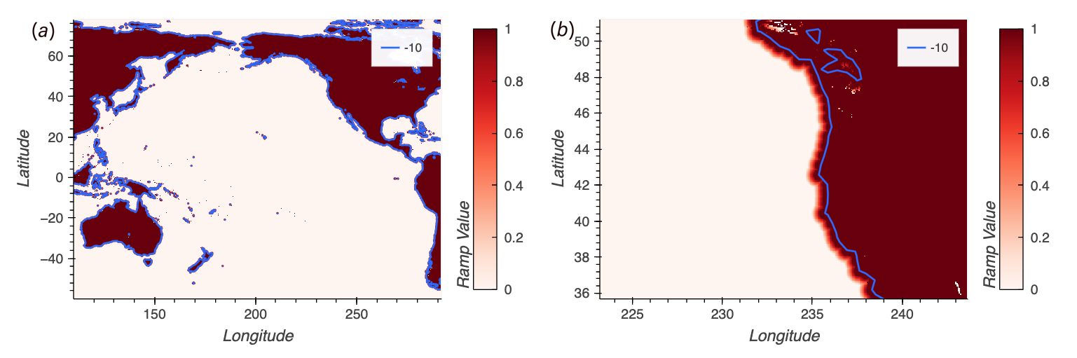
Figure 5 (a) Ramp function used to smooth transition the original grid to the Gaussian smooth grid. (b) Enlarged view of the ramp function along the United State's West Coast. Blue contour line denotes the 10 meter depth contour in both panels.

For both cases, NOAA and USGS, FUNWAVE simulations were performed using the bed deformation as the initial free surface water height. Figure 6 depicts the time history of generation and propagation of tsunami waves in the computational domain for the NOAA case with zero initial velocities. Simulations initialized with velocities from the elastic half-space model overestimate wave heights at DART stations for both the NOAA and USGS cases. In contrast, simulations with zero initial velocities provide more accurate predictions of wave heights at the DART locations (disregarding the phase lag), exhibiting minimal over-prediction or under-prediction of wave heights. This result indicates that within the framework of Boussinesq-type models like FUNWAVE, the initial bed-deformation is sufficient for effectively modeling tsunami wave propagation accurately.

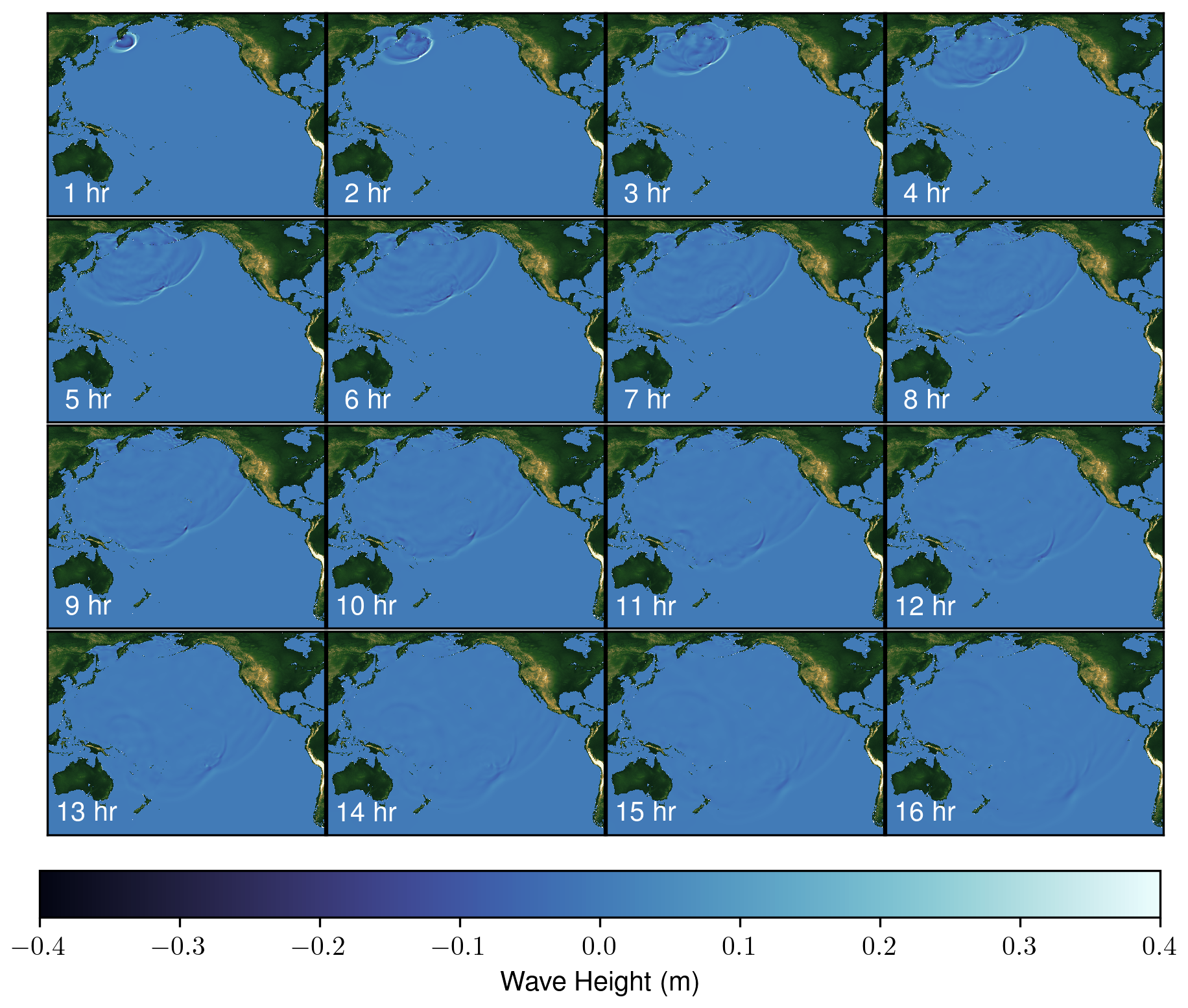
Figure 6 Free surface height (η) from FUNWAVE simulation initialized with bed deformation from NOAA scenario. Simulation results are shown at 1 h intervals across the panels.

Phase lag correction

Standard Boussinesq models assume an incompressible ocean over a rigid bed, causing theoretical phase speed overestimations and earlier arrivals, with the effect amplified at distant stations. To correct this bias, we quantified and applied a kinematic time-shift to the model outputs, without adjusting the hydrodynamic wave amplitudes. We utilize the formulation by Abdolali et al. (2019) and Abdolali and Kadri (2026), which incorporates water compressibility, Earth elasticity, and background density to calculate accurate phase speeds. These values were incorporated into a shortest-path framework (Kadri et al., 2025) to compute precise arrival times. Figure 7 illustrates this correction, displaying the travel times and the calculated time lag between the standard and compressible-ocean formulations. These differences (listed in Fig. 8c) at the DART sites were used to shift the FUNWAVE outputs, aligning modeled arrivals with observations (Fig. 8a).

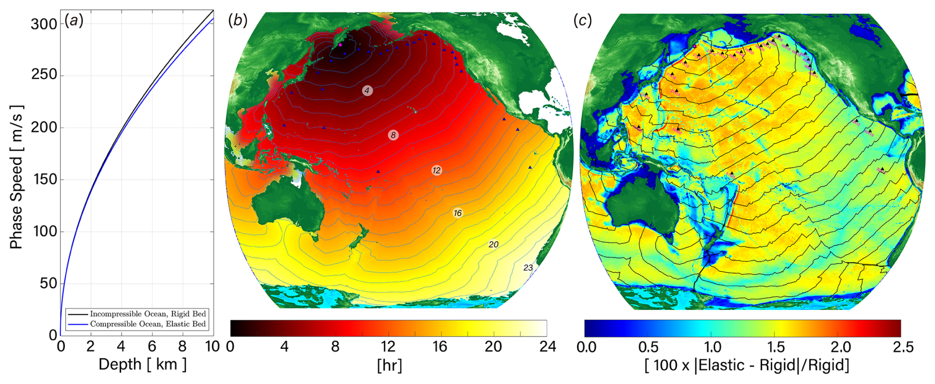
Figure 7 (a) Phase speed from the classic dispersion relation for an incompressible ocean over a rigid bottom (black) and for a compressible ocean with an elastic bottom and background density (blue); (b) surface gravity wave travel time derived from the blue curve in panel (a); black contours show travel time at 1 h intervals; (c) percentage reduction in phase speed between the black and blue curves in panel (a); black contours show the difference in travel time between the two dispersion relations at 1 min intervals.

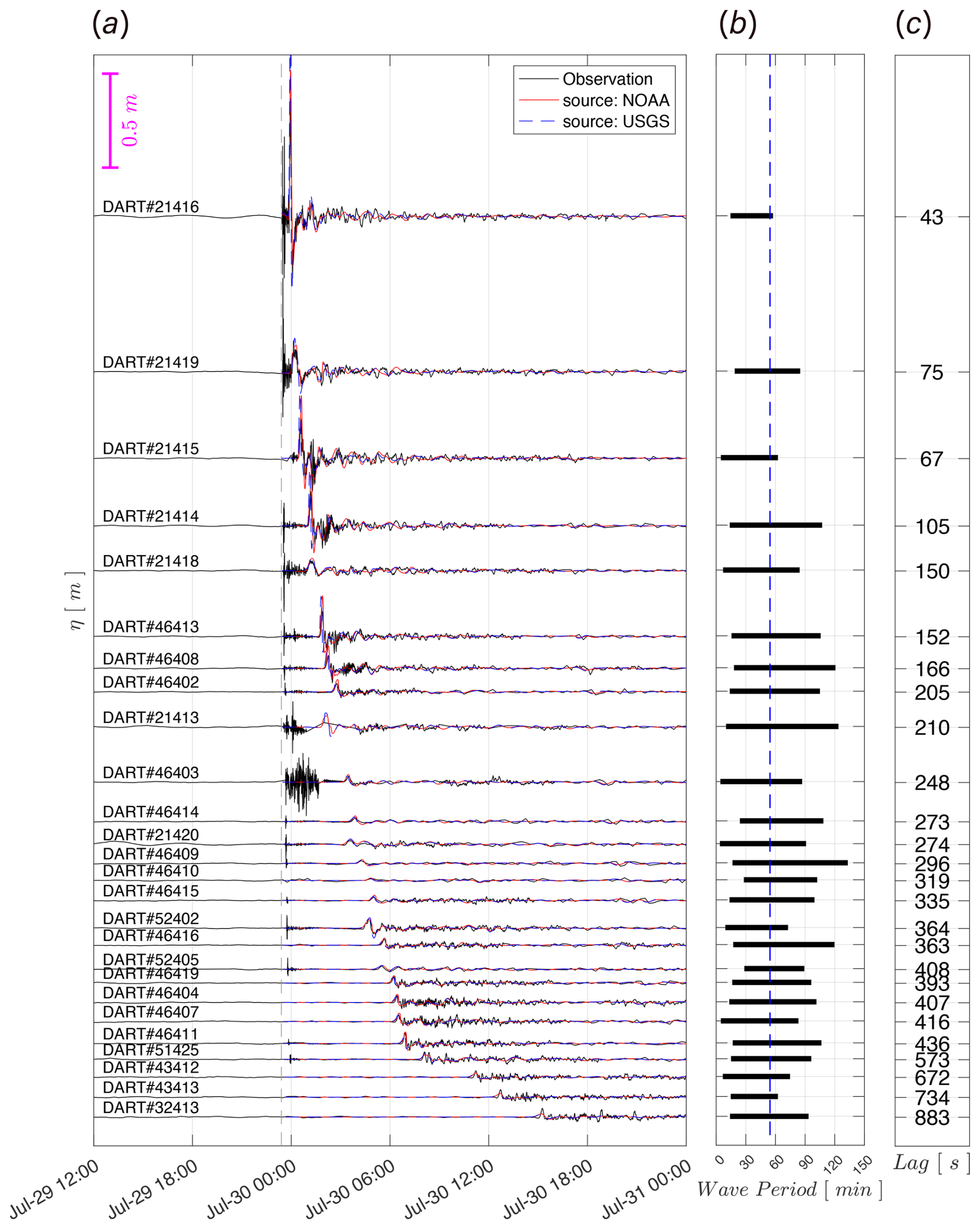
Figure 8 (a) Time series at DART observatories (black), with FUNWAVE simulations forced by the NOAA fault scenario (red) and the USGS scenario (blue). Stations are ordered by distance from the epicenter (magenta star in Fig. 7). The locations of the DART buoys are shown in Fig. 7. The vertical dashed line marks the earthquake origin time. (b) Estimated range of tsunami wave periods at all stations. The vertical dashed blue line indicates the overall mean period (∼ 60 min), used in the phase speed calculation. (c) Time lag between computed arrivals based on the standard dispersion relation and those incorporating ocean compressibility, Earth elasticity, and background density. The FUNWAVE results in panel (a) are shifted according to the values in panel (c).

Statistical analysis of phase-lag-corrected FUNWAVE outputs at DART stations demonstrates that the model effectively captures the tsunami signals generated by both source scenarios, with superior performance achieved using the NOAA fault configuration. The NOAA-forced simulation yields a Root Mean Square Error (RMSE) of 0.057, approximately 35 % lower than the USGS RMSE of 0.088, indicating a substantially smaller overall prediction error. Furthermore, the NOAA solution exhibits higher model fidelity, characterized by a Skill Factor of 0.955 and a low Scatter Index (SI) of 0.151, compared to the USGS scenario, which produced a Skill Factor of 0.915 and a significantly larger SI of 0.380.

4.2 Spatial Exposure Assessment

With the hydrodynamic model successfully validated against DART observations, we now evaluate the spatial distribution of tsunami energy across the Pacific basin. This step bridges the probabilistic and geometric frameworks outlined in Sects. 2 and 3 with the deterministic, high-fidelity simulation of the 2025 Kamchatka Peninsula event.

To evaluate the predictive capability of the ray-tracing framework, the model was initialized using the fault parameters of the Kamchatka event (NOAA scenario) listed in Table 2. A total of 270 rays were emitted perpendicular to the 540 km fault line (strike 217°) with a 3200 s (∼ 53 min) characteristic period, enabling a realistic representation of the initial radiation pattern, and were then tracked across the Pacific basin to identify convergence zones.

The resulting normalized ray termination counts are shown in Fig. 9a. Note that ray-based shadow zones appear sharper because diffractive spreading is absent in geometric optics. The simulation reveals clear corridors of energy focusing. In the near-field, high ray densities emerge along the Aleutian Islands and Alaska, primarily governed by the fault orientation and source proximity. In the far-field, bathymetric refraction organizes tsunami propagation into a dominant southeastward beam that first targets the Hawaiian Islands and then continues into the Southeast Pacific, ultimately forming a coherent refractive corridor that extends southward toward the coast of Chile. A second beam projects eastward toward the North American coast, notably targeting Washington, Oregon, and Northern California.

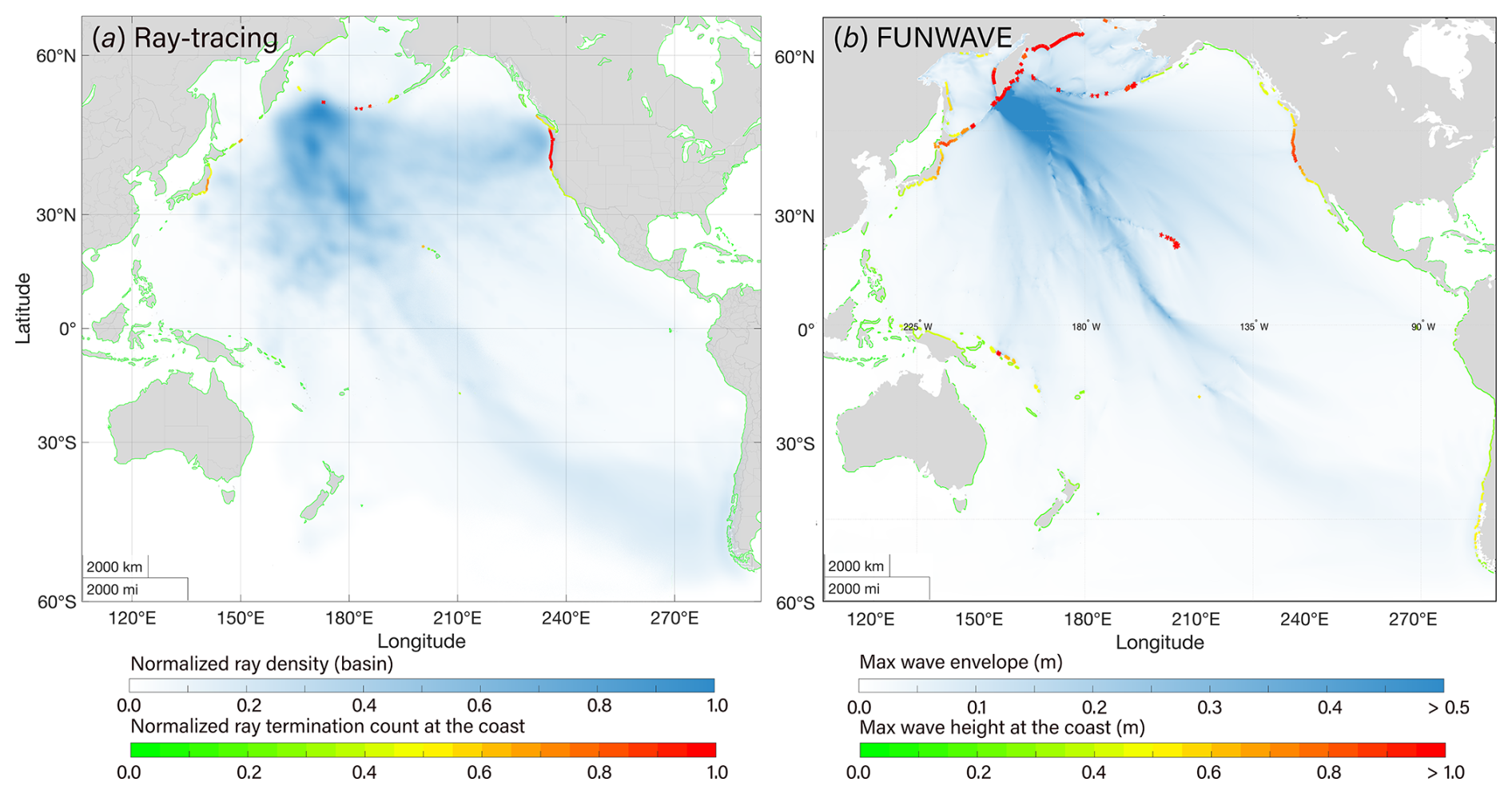
Figure 9 (a) Basin-wide ray density and coastal tsunami exposure derived from the ray-tracing model, where the coastline metric is a normalized ray-count proxy (0–1); (b) maximum free-surface elevations from FUNWAVE simulations for the 2025 Kamchatka Peninsula event, with the basin-wide field shown using the white–blue colormap and coastline segments using the green–yellow–red colormap. Basemap created with Natural Earth data.

These geometric patterns are strongly supported by the full hydrodynamic simulation. Figure 9b shows the maximum wave amplitude envelope computed by FUNWAVE. The spatial distribution closely aligns with the convergence zones identified in panel (a), while also capturing additional physical processes absent in the ray-tracing model. First, the ray-based simulation produces sharp shadow zones behind island chains (e.g., southeast of Hawaii), an expected consequence of its geometrical optics approximation. In contrast, FUNWAVE shows softer gradients, where diffraction allows partial energy penetration into these shadow regions. Second, the hydrodynamic solution reveals faint concentric ripples radiating from the continental margins-reflected energy that is naturally captured in FUNWAVE but purposely omitted in the ray-tracing model, where rays terminate upon coastal impact.

While a strong qualitative agreement is visually evident in the spatial alignment of energy corridors shown in Fig. 9, we further evaluated the model's performance statistically. To evaluate far-field predictive performance against the fully coupled FUNWAVE hydrodynamic simulations, a Spearman rank correlation was calculated for spatially co-located coastal amplitude distributions. To isolate far-field refractive propagation from localized static coseismic deformation, 161 coastal observation points were retained after explicitly excluding all points within a 1000 km radius of the epicenter, yielding a baseline correlation of ρ = 0.65.

Because standard significance testing ignores the spatial autocorrelation of coastal tsunami amplitudes, a spatial block-bootstrap resampling scheme was implemented to estimate unbiased confidence bounds. The remaining coastline was partitioned into contiguous 500 km segments along the coastal trajectory, which were randomly sampled with replacement over 10 000 iterations to preserve local spatial dependence. This methodology yielded an unbiased 95 % confidence interval of [0.35,0.83]. Because the confidence bounds remain strictly positive, the correlation is statistically significant (p < 0.01). Sensitivity analyses across 300 to 800 km block sizes confirmed that while confidence interval widths scale inversely with effective degrees of freedom, the lower bounds remain confidently above zero, confirming that the correlation is robust and independent of the selected bin size. Ultimately, despite underpredicting amplitudes in diffraction-dependent coastal shadow zones, the spatially adjusted analysis confirms a highly significant, physical monotonic relationship between the rapid screening predictions and high-resolution hydrodynamic benchmarks in the far-field.

Finally, these modeled hotspots are corroborated by in-situ observations. Figure 10 presents the maximum water levels recorded at NOAA tide gauge stations. The observational record exhibits strong agreement with both the ray-tracing and hydrodynamic models. The highest amplitudes (red and orange markers) occur precisely where both frameworks predicted energy focusing – along the Hawaiian Islands and the U.S. West Coast. Importantly, the secondary southern beam identified in both the ray-tracing solution (Fig. 9a) and the hydrodynamic envelope (Fig. 9b) is confirmed by an elevated water level at a gauge in the Southeast Pacific (Fig. 10), demonstrating the model's ability to resolve narrow, refractive transoceanic pathways over great distances.

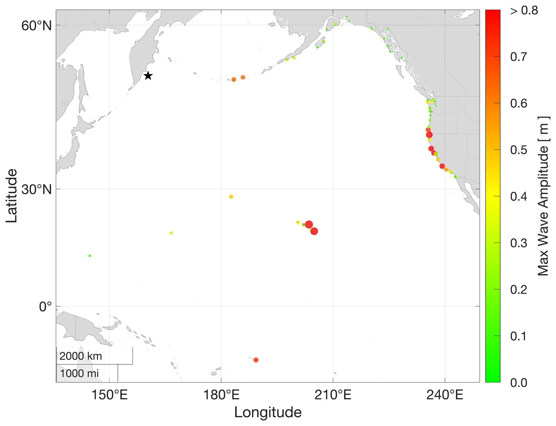
Figure 10 Maximum observed water levels at NOAA tide gauge stations along the coastline. Basemap created with Natural Earth data.

Collectively, these results show that when informed by accurate source mechanics, the ray-tracing framework serves as a robust and computationally efficient proxy for identifying far-field coastal exposure and quantifying basin-scale tsunami exposure.

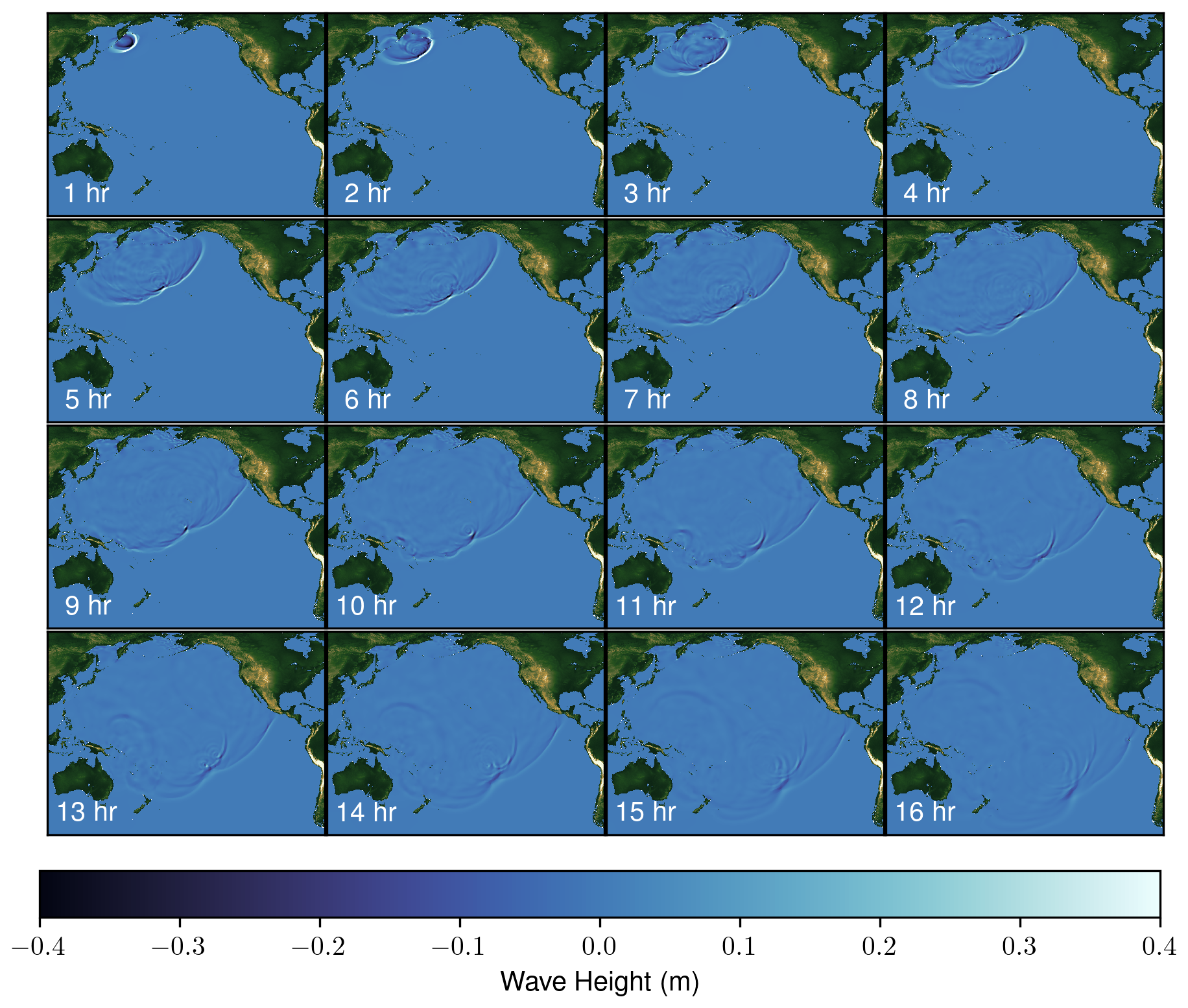
Figure 11 Spatiotemporal snapshots of the free surface height (η) simulated in FUNWAVE at 1 h intervals, illustrating the highly directional far-field energy beaming across the Pacific Ocean (Kirby et al., 2013).

5 2011 Tohoku-oki Tsunami

As a second case study, we apply the proposed ray-tracing framework to the 11 March 2011, M_w 9.0 Tohoku-oki megathrust earthquake to evaluate its performance under a different fault rupture geometry and source configuration. This event generated one of the largest trans-Pacific tsunamis ever recorded, characterized by highly directional energy radiation and pronounced far-field energy beaming across the Pacific Ocean (Kirby et al., 2013; Abdolali and Kirby, 2017). Figure 11 shows snapshots of the simulated free-surface elevation during the first 16 h of propagation, illustrating the strong directivity of the tsunami wave field as it traverses the Pacific basin.

Time series analyses of deep-ocean observations indicate a dominant mean wave period of approximately 35 min across the Pacific DART buoy network (Abdolali et al., 2019). Using the phase-lag correction procedure described in Sect. 4.1.1, this dominant wave period was used to correct the high-fidelity FUNWAVE simulations. The phase correction successfully aligned the modeled tsunami arrivals with the real-time de-tided observations recorded at DART stations throughout the Pacific (Fig. 12).

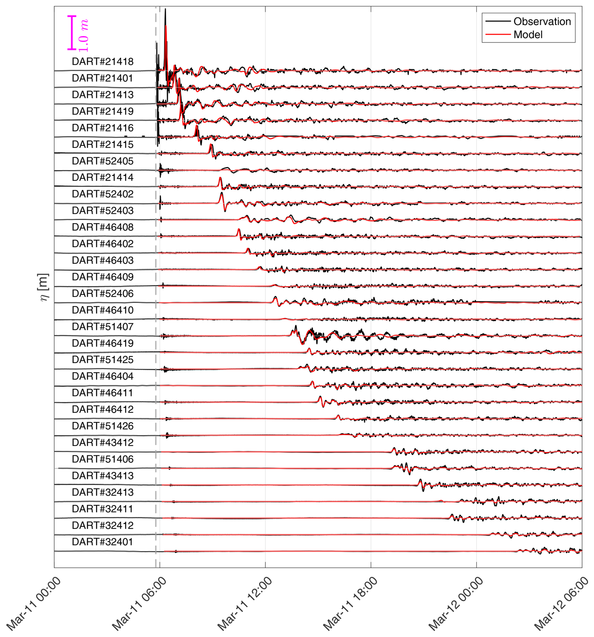
Figure 12 Validation of phase-lag-corrected FUNWAVE hydrodynamic simulations (red) against de-tided observations (black) recorded at deep-ocean Pacific DART stations (Abdolali et al., 2019).

We next evaluate the spatial exposure using the geometric ray-density metric described in Sect. 4.2. Figure 13 compares the normalized ray-count distribution with the maximum free-surface elevation obtained from the baseline FUNWAVE simulation. The ray-tracing framework successfully reproduces the primary regions of tsunami energy concentration and coastal exposure associated with this event. The spatial block-bootstrap analysis resulted in a correlation coefficient of ρ = 0.631 (95 % CI: 0.36–0.77, p < 0.01), demonstrating statistically significant agreement between the rapid geometric proxy and the full hydrodynamic solution. These results further confirm that the proposed unstructured ray-tracing approach provides a computationally efficient and robust framework for rapid tsunami exposure assessment across different fault geometries and ocean-basin scales.

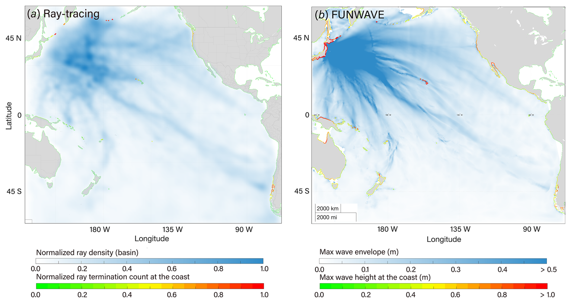
Figure 13 Comparison of the 2011 Tohoku-oki event showing (a) normalized ray-count proxy (0–1) and (b) the baseline FUNWAVE maximum wave envelope (η_max). Basemap created with Natural Earth data.

6 Conclusions

This study introduced a hybrid probabilistic–geometric framework, intended for rapid far-field exposure screening rather than local inundation modeling, that bridges the gap between statistical seismic exposure assessment and physically grounded tsunami propagation modeling. By integrating earthquake recurrence statistics derived from the Gutenberg–Richter relation with basin-scale ray-tracing, the method efficiently maps global patterns of energy convergence and identifies coastlines most susceptible to transoceanic tsunami exposure. This approach provides a rapid, computationally scalable alternative to full hydrodynamic ensemble modeling, making it suitable for global screening and early-stage exposure prioritization.

The framework was rigorously validated using the 2025 M 8.8 Kamchatka Peninsula earthquake as a benchmark case. Phase-corrected FUNWAVE simulations showed strong agreement with in-situ DART and tide-gauge observations, confirming that the hydrodynamic model, when corrected for compressibility, earth elasticity and background density, reproduced the key timing and amplitude characteristics of the event. Building on this foundation, the ray-tracing model, initialized with the optimized NOAA source parameters, successfully resolved the dominant transoceanic energy trajectories. Both the ray-tracing and hydrodynamic models identified the primary focusing pathway toward Hawaii and the U.S. West Coast, as well as the refraction-driven beam directed toward Chile.

The comparative analysis highlighted both the utility and the physical limitations of the geometric approach. While the ray-tracing model accurately predicted the location of far-field hotspots, it produced sharp shadow zones that neglected the diffraction effects captured by the weakly dispersive hydrodynamic model. Despite this approximation, the spatial alignment of maximum energy envelopes across observations, FUNWAVE simulations, and ray clusters, quantified by a Spearman correlation of ρ = 0.66, demonstrates that bathymetric refraction is the primary mechanism governing basin-scale tsunami intensity distribution.

Ray-tracing, weighted by recurrence-based probability, directly addresses the need for scalable exposure assessment. By filtering theoretical energy exposure through the lens of recurrence likelihood, the model provides a prioritized map of coastal regions where tsunami impacts are both physically focused and statistically probable. This combination offers a robust practical utility for coastal resilience, as consistently identified along high-energy refraction pathways can be flagged for focused vulnerability assessment and the allocation of high-fidelity modeling resources.

To date, many new construction initiatives along the coastlines require design analysis against both the extreme weather hazards and seismic-generated wave flooding events. Frameworks like those described in this manuscript can give rise to improved operational utility and creation of a single pane of glass, or a system of systems for hazard mitigation. In summary, this work demonstrates that a probabilistic–geometric approach serves as a defensible and efficient proxy for global tsunami exposure assessment, guiding decision-makers toward the communities facing the highest likelihood of future transoceanic impact.

Appendix A: Supplementary figures

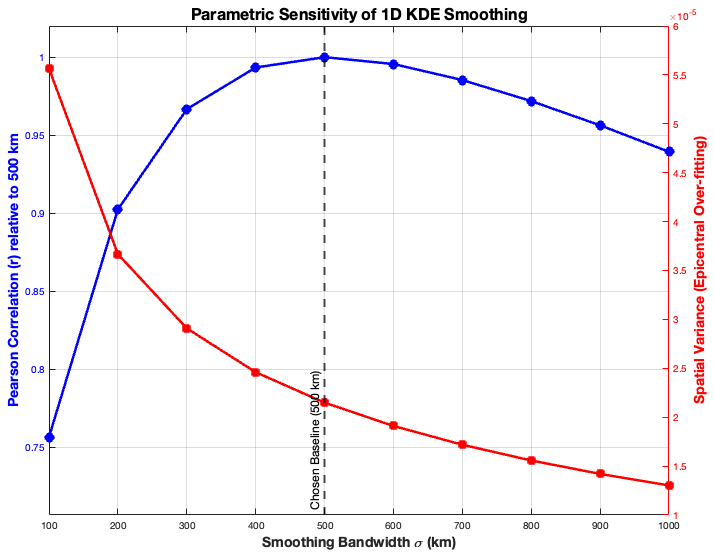
Figure A1 Parametric sensitivity of the 1D Kernel Density Estimation (KDE) smoothing bandwidth (σ). The red curve (right axis) shows spatial variance; values stabilize at the 500 km baseline, consistent with characteristic rupture lengths of great (M_w 8.8–9.0) megathrust events. The blue curve (left axis) shows the Pearson correlation coefficient (r > 0.95) relative to the 500 km baseline, demonstrating geographic stability across the bandwidth spectrum.

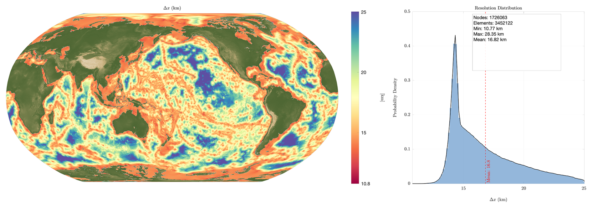
Figure A2 Spatial distribution and statistical properties of the variable-resolution unstructured ray-tracing mesh. (Left) Global map of the element sizes (Δx in km) demonstrating the feature-tracking nodal generation. Finer resolutions (red/yellow, ∼ 10.8–15 km) are explicitly forced along high-gradient bathymetric features such as seamount chains, mid-ocean ridges, and subduction trenches to preserve critical refractive boundaries. Coarser resolutions (blue, up to 28.35 km) are restricted to relatively flat abyssal plains. (Right) Probability density distribution of the element sizes, detailing the specific mesh geometry of 1 726 063 nodes and 3 452 122 elements with a mean resolution of 16.82 km.