Use of nonlinear principal components of CHIRPS precipitation data and ocean–atmospheric variables for streamflow forecasting in an area of scarce data – case study: Tocaría river basin – Orinoquia Colombiana

Accurate streamflow forecasting is essential for mitigating hydrological extremes and supporting sustainable water-resources management, particularly in data-scarce tropical catchments. This study proposes a hybrid forecasting framework that integrates Seasonal Autoregressive Integrated Moving Average models with exogenous inputs (SARIMAX), nonlinear principal components (NLPCs) derived from CHIRPS precipitation data, and large-scale ocean–atmosphere indices (macroclimatic variables, MVs). Four monthly models were developed and evaluated for the Tocaría River basin in the Colombian Orinoquía region: (1) a SARIMA (4,0,4)(0,0,3)12 model; (2) SARIMAX with MVs; (3) SARIMAX with NLPCs; and (4) a hybrid SARIMAX combining both MVs and NLPCs. All models were assessed using both raw and log-transformed streamflow data and benchmarked against simple baseline approaches. The hybrid model fitted to log-transformed streamflow showed consistent skill during both validation and testing (R² = 0.49 and 0.55, respectively), providing the most accurate reproduction of peak-flow conditions (lowest RMSE = 60.8 m³ s⁻¹). Skill was also maintained over longer lead times: for forecasts up to 24 months ahead, RMSE remained below 50 m³ s⁻¹ and R² remained above 0.80 across the forecast horizon. These results underscore the effectiveness of integrating nonlinear precipitation patterns, macroclimatic variability, and temporal dependence to improve forecast accuracy under data-scarce conditions, particularly for peak flows and anomalously wet periods that are not adequately captured by the climatological benchmark. The proposed methodology offers a transferable approach for operational forecasting in ungauged or sparsely monitored basins, contributing to early warning systems, drought preparedness, and adaptive water governance in vulnerable tropical regions.

1 Introduction

Sustainable management of water resources in tropical basins critically depends on the ability to anticipate streamflow dynamics accurately under complex hydroclimatic variability. Streamflow integrates precipitation, evapotranspiration, infiltration, and climatic anomalies across multiple spatial and temporal scales, yet sparse hydrometeorological monitoring limits the characterization of these processes (Tootle et al., 2008; Yao et al., 2020).

Conventional statistical models such as Autoregressive Integrated Moving Average (ARIMA) and its seasonal extension (SARIMA) have been widely applied to streamflow prediction because of their ability to represent temporal dependencies and seasonality under stationarity assumptions (Sirisha et al., 2022; Valipour, 2015). However, their performance diminishes when abrupt, nonlinear fluctuations characteristic of tropical catchments influenced by exogenous climate drivers must be captured (Moeeni and Bonakdari, 2017). Previous studies have shown that incorporating exogenous variables into forecasting models significantly enhances streamflow prediction skill, particularly at seasonal to interannual timescales, by explicitly accounting for external climate-forcing mechanisms (Wong et al., 2007).

In regions such as the Colombian Orinoquía, the interplay of large-scale ocean–atmosphere phenomena, especially the El Niño-Southern Oscillation (ENSO), introduces pronounced nonstationarity and nonlinearity, thereby challenging traditional time-series forecasting methods (Chiew and McMahon, 2002; Pasquini and Depetris, 2007; Yap and Musa, 2023). Models incorporating macroclimatic indices, such as sea surface temperature anomalies and ENSO-related indices, have demonstrated substantial improvements in streamflow forecasting accuracy for Andean and Pacific basins (Cárdenas-Rodríguez et al., 2022; Mesa et al., 2001; Poveda et al., 2002; Velásquez et al., 2010). Nevertheless, similar studies remain scarce for the Orinoquía region, despite its hydrological sensitivity to both Pacific and Atlantic climatic influences (Builes-Jaramillo et al., 2022). The Tocaría River basin in the Colombian Orinoquía exemplifies this knowledge gap, as it is characterized by limited hydrometeorological instrumentation and experiences seasonal extremes of drought and flooding that affect local agriculture and ecosystems (Corporinoquia and Corpoboyacá, 2015a).

Building on previous work that successfully employed Nonlinear Principal Component Analysis (NLPCA) combined with satellite-derived Climate Hazards Group InfraRed Precipitation with Station data (CHIRPS) to impute missing monthly streamflow records in the Tocaría basin, demonstrating high accuracy across stations with substantial data gaps (Ocampo-Marulanda et al., 2025), this study advances the development of a parsimonious hybrid forecasting framework. The proposed SARIMAX model integrates a SARIMA component with NLPCs derived from CHIRPS data and MVs representing large-scale atmosphere-ocean drivers.

This research aims to provide an accurate monthly streamflow forecasting tool tailored to the hydrological regime of the Tocaría River, thereby supporting adaptive water-resources management in a data-limited and climate-vulnerable tropical basin. By addressing key gaps in scientific knowledge and practical decision-support tools, the framework offers scalable potential for application in other similarly under-monitored tropical catchments subject to complex climatic forcing.

2 Methodology

This section outlines the methodological framework developed for monthly streamflow forecasting in poorly instrumented basins, using the Tocaría River (Colombian Orinoquía) as a case study. The approach integrates seasonal autoregressive modeling with exogenous predictors, nonlinear dimensionality reduction, and multivariate correlation analysis.

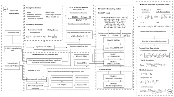
Figure 1 Schematic overview of the methodological workflow, including input data preprocessing, determination of the predictor pool, streamflow forecasting, and performance evaluation of the best-performing model.

As illustrated in Fig. 1, the methodological workflow integrates input-data preprocessing, SARIMA order selection, and determination of the predictor pool. Subsequently, 4 SARIMA-based streamflow forecasting models were independently trained, validated, and tested. All models were evaluated using both raw and log-transformed streamflow data and benchmarked against simple climatology and persistence baselines. Predicted values were assessed using the Root Mean Square Error (RMSE), the coefficient of determination (R²), the Akaike Information Criterion (AIC), and the Bayesian Information Criterion (BIC). Finally, for the best-performing model, forecast-error degradation across increasing prediction horizons was analyzed and a comprehensive residual analysis was conducted.

Figure 2 Geographic location of the Tocaría River basin and El Playón hydrometric station. Digital elevation model, political boundaries, watershed boundaries, and rivers extracted from GEOPORTAL IDEAM: https://visualizador.ideam.gov.co (last access: 21 November 2024).

2.1 Study area

The Tocaría River originates at 3200 m above sea level on Guevarrica Hill and drains a watershed of 2223 km² on the eastern flank of the Eastern Cordillera. The river extends for 127.5 km and has an average longitudinal slope of 5 %. The basin is part of the Cravo Sur system, a tributary of the Meta River within the Orinoco macro-basin (Corporinoquia, 2010; Corporinoquia and Corpoboyacá, 2015b) (Fig. 2).

The basin experiences a monomodal rainfall regime with a distinct wet season from April to November and a dry season from December to March. Although 90 % of the basin lies within the Andean region, its discharge contributes to the Orinoquía domain. Mean annual precipitation is approximately 2031 mm, with peak streamflows during the wet season and minimum flows in February (Ruíz-Ochoa et al., 2022; Urrea et al., 2016).

2.2 Data

Three main datasets were used for model development: observed streamflow, CHIRPS precipitation, and macroclimatic variables.

Streamflow data were obtained from the El Playón station, operated by Colombia's national hydrometeorological institute (IDEAM), for the period 1983–2019, with approximately 5 % missing values. Data were sourced from the DIHME geoportal (http://dhime.ideam.gov.co, last access: 13 January 2025), and the missing values were imputed using an NLPCA approach that incorporated CHIRPS precipitation data as an exogenous input, following the methodology described in greater detail by Ocampo-Marulanda et al. (2025).

Figure 3 Monthly streamflow climatology at the El Playón station, Tocaría River.

Mean monthly discharge was 92.4 m³ s⁻¹, with strong seasonal variability: February averaged 17 m³ s⁻¹ (the driest month), whereas July peaked at 177 m³ s⁻¹ (Fig. 3). These fluctuations highlight the need for modeling strategies capable of capturing both hydroclimatic seasonality and interannual variability.

Satellite-based precipitation data were obtained from CHIRPS, which integrates satellite and in situ observations. CHIRPS provides global coverage at 0.05° spatial resolution from 1981 to the present. Its performance in Colombia is well documented (Funk et al., 2014; Urrea et al., 2016; Ocampo-Marulanda et al., 2022). In this study, 81 CHIRPS time series corresponding to 81 grid cells located within the Tocaría River basin were used.

Macroclimatic variables were retrieved from the National Oceanic and Atmospheric Administration (NOAA, https://psl.noaa.gov/gcos_wgsp/, last access: 17 January 2025). 21 indices representing sea surface temperature anomalies, atmospheric pressure, and wind patterns were selected on the basis of previously demonstrated correlations with Colombian streamflow regimes (Canchala et al., 2020a; Cerón et al., 2020; Poveda et al., 2011). Complete descriptions of the selected variables are provided in Table S1 in the Supplement.

2.3 Data preprocessing

This subsection details the statistical preprocessing applied to the streamflow data prior to model development, including variability characterization, trend detection, structural-change identification, and stationarity assessment. All analyses were conducted in Python. Data processing and manipulation were carried out using pandas and NumPy, while statistical and time-series analyses were performed using SciPy and statsmodels. The NLPCA analysis was implemented using scikit-learn and TensorFlow.

2.3.1 Descriptive statistics and trend analysis

Descriptive statistics included the mean, maximum, standard deviation, and coefficient of variation (CV), providing an initial quantification of streamflow magnitude and variability. Structural changes were identified using Pettitt's test (Pettitt, 1979), which revealed a significant breakpoint in the time-series mean. Sen's slope estimator (Sen, 1968) quantified long-term trends, while the Mann–Kendall test (Mann, 1945) evaluated trend significance.

2.3.2 Stationarity assessment

Stationarity was explored through additive time series decomposition using classical seasonal decomposition based on moving averages, which separates the series into trend, seasonal, and residual components, enabling visual inspection of long-term behavior, seasonal structure, and residual stability. Subsequently, stationarity was formally evaluated using the Phillips–Perron (PP) test, which tests the null hypothesis of a unit root and is robust to autocorrelation and heteroskedasticity in the residuals.

2.3.3 Autocorrelation and partial autocorrelation

Temporal dependencies were examined using autocorrelation function (ACF) and partial autocorrelation function (PACF) analyses (Chatfield, 1989). The ACF quantifies the linear correlation at lag k and is defined as:

$$\begin{array}{}\text{(1)}& r_k={\displaystyle \frac{{\sum }_{t=\mathrm{1}}^{n-k}(x_t-\stackrel{\mathrm{‾}}{x})(x_{t+k}-\stackrel{\mathrm{‾}}{x})}{{\sum }_{t=\mathrm{1}}^{n-k}(x_t-\stackrel{\mathrm{‾}}{x}{)}^{\mathrm{2}}}},\end{array}$$

where x_t is the series value at time t, $\stackrel{\mathrm{‾}}{x}$ is the mean, and n is the number of observations.

PACF measures correlation at lag k controlling for intermediate lags, informing autoregressive and moving average term selection in SARIMA models (Box et al., 2015). ACF and PACF plots were examined for seasonality and persistence, using 95 % confidence intervals to identify significant lags.

2.4 Selection of potential predictors

2.4.1 CHIRPS precipitation as a predictor

The hydrological relationship between precipitation and streamflow in the Cravo Sur basin has been previously demonstrated (Ocampo-Marulanda et al., 2025), supporting the use of CHIRPS precipitation data as potential predictors. In this study, 81 precipitation time series corresponding to CHIRPS grid cells within the Tocaría sub-basin were analyzed and reduced in dimension to extract the main information contained in this dataset (Xn) using an NLPCA approach. The nonlinear principal components (NLPCs) obtained in the bottleneck layer of the NLPCA model (ym) represent the main modes of precipitation variability in the region. For this purpose, a Multi-Layer Perceptron (MLP) neural network was used, with an input layer, one or more hidden layers, and an output layer. During training, the back-propagation algorithm was used to identify the optimal combination of synaptic weights by minimizing reconstruction error through iterative updates of weights and bias terms. Several network topologies were evaluated, and the [81-2-81] architecture produced the best results; the components were estimated in hierarchical order. Linear activation functions were used for the hidden and output layers, and the best performance was obtained after 100 training epochs.

The nonlinear principal components were estimated using only the 70 % subset of precipitation data corresponding to the SARIMAX model training period (1985–2008), as defined in Sect. 2.5. Implemented through an autoencoder with bottleneck architecture, NLPCA minimizes the reconstruction error between inputs and outputs, thereby capturing nonlinear relationships beyond the capabilities of traditional PCA (Canchala et al., 2019; Scholz et al., 2007). Validation of the extracted components included reconstruction accuracy and latent-space visualization, confirming their effectiveness in summarizing precipitation variability.

2.4.2 Macroclimatic variables as large-scale predictors

MVs comprising sea surface temperature anomalies, sea-level pressure, and wind indices known to influence Colombian hydrology (Canchala et al., 2020a, b; Cerón et al., 2020; Poveda et al., 2001) were evaluated.

Spearman rank correlations between each MV and streamflow were calculated for lags of up to 14 months to capture delayed effects. Variables exhibiting statistically significant correlations at lags ≥ 6 months were retained, reflecting hydroclimatic memory. Only predictors with demonstrated hydrological relevance and minimal intercorrelation were preserved to ensure model parsimony and stability.

2.4.3 Multicollinearity diagnosis and variable selection

A two-step screening procedure was applied to select the exogenous predictors used in the forecasting models. First, pairwise correlation matrices visualized as heatmaps were used to identify groups of highly correlated MVs, thereby detecting potential redundancy among predictors and identifying those most strongly associated with streamflow (Dormann et al., 2013). Second, the Variance Inflation Factor (VIF) was computed to quantify multivariate collinearity among the candidate predictors (Katrutsa and Strijov, 2017).

Predictors with VIF values greater than 10 were considered excessively collinear and were iteratively removed. When several variables conveyed similar large-scale climatic information, selection was guided not only by the reduction of VIF values but also by the strength of their absolute correlation with streamflow, in order to retain the predictor with the most hydrologically relevant signal while preserving model parsimony. After each elimination step, VIF values were recalculated until the reduced predictor set showed acceptable multicollinearity levels.

2.5 Forecasting model: SARIMAX architecture

The forecasting approach proposed herein is based on a hybrid SARIMAX framework that integrates nonlinear temporal dynamics, exogenous climatic forcings, and seasonal variability within a unified predictive architecture.

The forecasted streamflow vector, denoted as $\widehat{y}\left(k\right)\in R^m$, is modeled as a nonlinear function of multiple lagged sequences:

Streamflow autoregressive terms:

$$\begin{array}{}\text{(2)}& y\left(k\right),y(k-\mathrm{1}),\mathrm{\dots },y(k-n_y)\end{array}$$

Exogenous forcings (e.g., ocean–atmospheric indices):

$$\begin{array}{}\text{(3)}& \begin{array}{rl}& u_{\mathrm{1}}\left(k\right),u_{\mathrm{1}}(k-\mathrm{1}),\mathrm{\dots },u_{\mathrm{1}}(k-n_{\mathrm{u}\mathrm{1}}),\mathrm{\dots };u_r\left(k\right),u_r(k-\mathrm{1}),\\ & \mathrm{\dots },u_r(k-n_{\text{ur}})\end{array}\end{array}$$

Forecast residuals:

$$\begin{array}{}\text{(4)}& e_k\left(k\right),e(k-\mathrm{1}),\mathrm{\dots },e(k-n_e)\end{array}$$

Seasonal lags of streamflow and residuals:

$$\begin{array}{}\text{(5)}& {\displaystyle }y(k-s),y(k-\mathrm{2}s),\mathrm{\dots },y(k-n_s\cdot s)\text{(6)}& {\displaystyle }e(k-s)e(k-\mathrm{2}s),\mathrm{\dots },e(k-n_s\cdot s)\end{array}$$

The model's general transfer function is expressed in Eq. (7):

$$\begin{array}{}\text{(7)}& \begin{array}{rl}& y(k+\mathrm{1})=fW\times \\ & \left[\begin{array}{c}y\left(k\right),y(k-\mathrm{1}),\mathrm{\dots },y(k-n_y);\\ u_{\mathrm{1}}\left(k\right),u_{\mathrm{1}}(k-\mathrm{1}),\mathrm{\dots },u_{\mathrm{1}}(k-n_{\mathrm{u}\mathrm{1}});u_r\left(k\right),u_r(k-\mathrm{1}),\mathrm{\dots },u_r(k-n_{\text{ur}})\\ e_k\left(k\right),e(k-\mathrm{1}),\mathrm{\dots },e(k-n_e)]\\ y(k-s),y(k-\mathrm{2}s),\mathrm{\dots },y(k-n_s\cdot s),\\ e(k-s),e(k-\mathrm{2}s),\mathrm{\dots },e(k-n_s\cdot s)\end{array}\right],\end{array}\end{array}$$

where the terms represent the autoregressive, exogenous, residual, and seasonal lag orders, respectively; s denotes seasonal periodicity; and f is a nonlinear mapping function parameterized by model weights.

This hybrid configuration enables simultaneous modeling of high-order dependencies, memory effects, and seasonal recurrence. Incorporating lagged residuals and seasonal components allows the model to capture patterns not accounted for by direct input–output relations, enhancing its capacity to learn both deterministic and stochastic dynamics.

An open-loop configuration was adopted during training, feeding observed streamflow values back to stabilize learning. For validation and operational forecasting, a closed-loop mode recursively propagates forecasted values. Residual sequences were standardized during validation and testing to ensure numerical stability.

The structure of the SARIMA model was determined through visual inspection of autocorrelation (ACF) and partial autocorrelation (PACF) plots of the monthly streamflow series. The orders ($p,d,q$) and ($P,D,Q$) were selected to reflect the presence of short-term dependencies and seasonal dynamics. Differencing was not applied, as the series appeared stationary in both its level and seasonal pattern. To support this assessment, the Phillips–Perron test was applied to evaluate the presence of unit roots and inform the choice of d=0 and D=0. A seasonal period of s=12 was defined based on the observed annual cycle in streamflow behavior.

Data were partitioned into 70 % training (1985–2008), 15 % validation (2009–2013), and 15 % testing (2014–2019) subsets, preserving temporal order to avoid information leakage. In addition to Bayesian regularization, early stopping was implemented by monitoring validation loss with a patience threshold of 100 epochs, halting training when performance ceased to improve.

2.6 Logarithmic transformation of streamflow

Monthly streamflow series often present positive skewness, heteroscedastic variance, and pronounced extremes associated with flood events, which challenge the assumptions of linear stochastic models such as SARIMA and SARIMAX. To address these issues, a logarithmic transformation was applied to the observed streamflow prior to model calibration:

$$\begin{array}{}\text{(8)}& y_t^{\text{log}}=\text{log}(y_t+\mathrm{1})\end{array}$$

This transformation stabilizes variance and improves the suitability of the series for linear time-series modeling. All SARIMA estimation and forecasting were performed in the log-transformed space. Forecasts were then back-transformed to the original scale to ensure physical interpretability:

$$\begin{array}{}\text{(9)}& \widehat{y_t}=e^{\left({\widehat{y_t}}^{\text{log}}\right)}-\mathrm{1}\end{array}$$

The transformation enhanced the model's ability to represent both low- and high-flow conditions, particularly under strong seasonal variability.

2.7 Evaluation of the models

2.7.1 Evaluation metrics and baselines

Model performance was first assessed using R² and RMSE for the training, validation, and test periods, alongside AIC and BIC to evaluate goodness-of-fit. These metrics provide a quantitative overview of how well each model reproduces the general behavior of the streamflow series.

Forecasts were then compared against simple baselines: monthly climatology, computed as the average flow for each month in the training period, and persistence, which assumes that the flow at time t equals the flow at time t−1. This comparison allows us to contextualize the added value of the SARIMAX model relative to straightforward, intuitive approaches.

Special attention was given to the evaluation of high flows, defined as events above the 90th percentile, by computing RMSE for these peaks. Since the SARIMAX model is designed to capture extreme events, this peak-focused analysis was prioritized to assess its skill in predicting the most critical conditions for water management.

Finally, 95 % confidence intervals were estimated for all forecasts. After fitting the model on log-transformed data with exogenous variables, predictions and confidence intervals were obtained in log scale and back-transformed to the original units. These intervals illustrate the uncertainty around the forecasted values, providing a clear sense of the expected range for future streamflow.

Table 1 Streamflow characteristics at El Playón station.

2.7.2 Forecast error degradation across prediction horizons

Forecasting accuracy typically decreases as the prediction horizon extends, a well-documented phenomenon referred to as forecast error degradation (Xiang et al., 2024). To assess this behavior, the best-performing SARIMAX model was evaluated over multiple lead times using RMSE and R² as performance metrics. Forecasts were produced for 2 to 24 months ahead in increments of 2 months, enabling the quantification of predictive accuracy across short, medium, and long term horizons.

To capture the evolution of forecast quality, RMSE and R² values were analyzed in pairs of consecutive horizons. This pairing facilitated the visualization of degradation trends through line plots, offering insights into the temporal limits of model effectiveness.

2.7.3 Residual analysis

Residual diagnostics are essential for evaluating model adequacy by verifying whether prediction errors conform to standard statistical assumptions. Residuals were computed as the difference between observed and forecasted streamflow values, forming a time series that was subjected to rigorous statistical and graphical analysis.

Normality was tested using the Jarque–Bera test (Jarque and Bera, 1980), assessing whether residuals follow a Gaussian distribution, a prerequisite for valid inference and uncertainty quantification. Autocorrelation was examined through the Durbin–Watson statistic (Durbin and Watson, 1950), where values near 2 suggest the absence of significant serial dependence, thus confirming that temporal structures have been effectively captured. Heteroscedasticity was assessed via the Breusch–Pagan test (Breusch and Pagan, 1979); significant p values indicated non-constant residual variance, potentially undermining the model's generalizability.

Complementing these tests, graphical diagnostics were employed to detect patterns indicative of model misspecification. Histograms with kernel density estimation (Silverman, 1986) were used to visually assess normality, while residuals-versus-fitted-values plots revealed heteroscedastic patterns or structural biases. Quantile-quantile plots (Wilk and Gnanadesikan, 1968) further evaluated the agreement between empirical and theoretical residual quantiles. Finally, ACF plots were used to identify lagged dependencies; the absence of significant peaks outside the confidence bounds supported the white-noise assumption.

3 Results and discussion

The experimental results are organized into three subsections: (1) description of the streamflow data, (2) determination of the predictor pool, and (3) the forecasted streamflow series. Each subsection presents and discusses the relevant findings, with emphasis on identifying the most suitable forecasting model on the basis of accuracy metrics. A comparative analysis of the 4 evaluated models highlights their strengths and limitations, guiding the selection of the most effective model for streamflow prediction.

Long-range streamflow forecasting is a valuable tool for water-resource managers because it enables proactive decision-making and strategic planning. However, extending the forecast lead time excessively tends to degrade model performance, often reducing predictive accuracy. Consequently, this study adopts a 24-month lead time to evaluate and compare forecasting models. This horizon provides a balance between planning requirements and achievable accuracy for watershed-management stakeholders.

3.1 Description of the streamflow data

3.1.1 Statistical and graphical description

The streamflow time series at El Playón station exhibits pronounced interannual and seasonal variability, with values ranging from 2.5 to 280 m³ s⁻¹ and a mean of 92.4 m³ s⁻¹. This range is consistent with the monomodal rainfall regime characteristic of the region (Urrea et al., 2016). A standard deviation of 66.4 m³ s⁻¹ and a coefficient of variation of 71.8 % confirm the high dispersion and temporal heterogeneity of the data, which pose a challenge for accurate modeling and prediction.

Figure 4 Temporal behavior of streamflow at the Tocaría River.

Trend-detection tests were also applied. Visual inspection suggested a potential breakpoint in January 2019; however, the Pettitt test yielded a p value of 1.00, indicating that this change is not statistically significant. Likewise, Sen's slope estimator and the Mann–Kendall test indicated a slight upward trend in discharge, but without statistical significance (p = 0.3445), suggesting the absence of a persistent monotonic trend (see Table 1 and Fig. 4).

These characteristics highlight the complexity of the time series and justify the need for rigorous preprocessing, including stationarity and autocorrelation analysis.

Figure 5 Decomposition of El Playón streamflow time series into trend, seasonality, and residual components.

3.1.2 Stationarity analysis

Stationarity was assessed through a combination of exploratory decomposition and formal statistical testing. Figure 5 presents the seasonal decomposition results. The trend component does not exhibit a persistent increasing or decreasing pattern over the analyzed period; instead, it shows multi-year fluctuations characterized by alternating phases of higher and lower streamflow. These variations suggest low-frequency hydroclimatic variability rather than a clear long-term trend, indicating that mean discharge remained broadly stable over time, although modulated by interannual and decadal variability.

Figure 6 Autocorrelation of the time series of El Playón streamflow for 100 months of lags.

The seasonal component displays a clear and regular periodicity, reflecting a 12-month seasonal cycle in streamflow. This pronounced seasonality is consistent with the regional hydroclimatic regime, dominated by the alternation between wet and dry seasons, and confirms that streamflow variability in the Tocaría River is largely controlled by seasonal precipitation patterns.

The residual component exhibits a random distribution centered around zero, with no discernible systematic patterns or trends. It captures short-term variability, extreme events, and noise not explained by the trend or seasonal components, supporting the adequacy of the seasonal decomposition and the assumption of weak stationarity after seasonal removal.

The Phillips–Perron test further confirmed stationarity, yielding a test statistic of −6.5005 and a p value < 0.0001, allowing rejection of the null hypothesis of a unit root. These results justify modeling without differencing and the selection of d=0 in the SARIMA model.

3.1.3 Autocorrelation and partial autocorrelation structure

The ACF displays significant periodic peaks at regular intervals, indicative of strong seasonal periodicity and persistent temporal dependencies beyond short lags (Fig. 6). This cyclicality aligns with hydrological patterns driven by seasonal precipitation and runoff dynamics, underscoring the appropriateness of seasonal forecasting models such as SARIMA.

Figure 7 Partial autocorrelation function of El Playón streamflow series over 25 monthly lags.

The PACF shows a prominent spike at lag 1 followed by rapid decay to values within the confidence bounds (Fig. 7), consistent with an autoregressive process of order 1 (AR(1)); however, the selected SARIMA model incorporates higher-order dynamics to capture the longer memory and seasonal structure identified in the ACF. The lack of significant PACF values at higher lags indicates limited benefit from additional autoregressive terms.

Based on combined ACF and PACF analysis, a SARIMA (4,0,4)(0,0,3)12 model was selected. This model configuration incorporates the identified seasonal periodicity (season length s=12), confirms stationarity (d=0), and captures short-term autoregressive and moving average dynamics. Residual diagnostics validated the model's adequacy, demonstrating no significant autocorrelation.

3.2 Determination of the pool predictors

3.2.1 Selection of precipitation NLPCs as exogenous variables

The 81 CHIRPS precipitation time series for the Tocaría River basin were compressed into two nonlinear principal components (NLPC1 and NLPC2) using an autoencoder-based NLPCA. The resulting latent scores showed variances of 17.64 (NLPC1) and 6.30 (NLPC2), corresponding to 73.69 % and 26.31 % of the variance within the two-dimensional latent space, respectively. These percentages describe the relative contribution of each latent coordinate. The two NLPCs were subsequently used as exogenous covariates in the streamflow forecasting model, providing a parsimonious representation of basin-scale precipitation variability. This approach is consistent with Ocampo-Marulanda et al. (2025), who used CHIRPS-derived nonlinear precipitation components as compact predictors for streamflow reconstruction in data-scarce basins.

3.2.2 Selection of macroclimatic variables as exogenous variables

The influence of 21 MVs on streamflow variability in the Tocaría River was assessed using a lagged Spearman correlation analysis, considering time lags from 0 to 14 months. This asynchronous framework allowed the identification of delayed relationships between climate anomalies and hydrological responses, which are crucial for predictive modeling. This  lagged-correlation framework enables the detection of delayed hydroclimatic teleconnections, which are essential for long-lead streamflow forecasting.

Figure 8 Lagged Spearman correlations between MVs and streamflow at El Playón station.

Statistical significance was evaluated using two-tailed tests with confidence levels between 90 % and 99 %. Figure 8 displays the lagged correlations between the MVs and streamflow at El Playón station. Several variables showed statistically significant correlations across multiple lags and exhibited a quasi-periodic structure that reflects the hydroclimatic seasonality modulated by the Intertropical Convergence Zone (ITCZ).

Key Pacific-related indices – namely NINO12 (ρ=0.75) and NINO3 (ρ=0.60) – emerged as the strongest predictors, underscoring the robust influence of ENSO-related sea surface temperature (SST) anomalies on the Tocaría River streamflow. These findings are consistent with previous studies across Colombia (e.g., Cadavid and Salazar, 2008; Canchala et al., 2020c; Poveda et al., 2002), which reported comparable lagged correlations between ENSO indices and regional streamflow, often with cyclic behavior.

In addition, Atlantic-related variables such as AMM (ρ=0.32) and TSA (ρ=0.25) showed statistically significant, albeit weaker, correlations. These results corroborate the relevance of Atlantic SST variability in eastern Colombia. The Llanos low-level jet and moisture transport from the tropical Atlantic – modulated by indices such as AMM and TSA – have been highlighted as key controls of precipitation and streamflow in the Orinoquía region (Correa et al., 2024; Builes-Jaramillo et al., 2022; Labat et al., 2012; Nieto et al., 2008).

The set of significantly correlated predictors spans both Pacific and Atlantic basins: NINO3, NINO4, NINO12, NINO34, PDO, TNI, NP, QBO (Pacific-related), and AMO, NTA, TNA, NAO, AMM, TSA (Atlantic-related). This reinforces the complexity of the climate–hydrology interactions in the Tocaría River basin and emphasizes the need to account for both direct and lagged macroclimatic signals in predictive modeling.

Figure 9 Correlation heatmap of predictor variables.

3.2.3 Assessing multicollinearity and variable selection for improved time series forecasting

The results of the correlation heatmap (Fig. 9) reveal substantial interdependence among several MVs, indicating that the inclusion of multiple closely related predictors may introduce redundancy and model instability. For instance, the ENSO indices NINO3, NINO4, NINO12, and NINO34 exhibit strong mutual correlations, suggesting that a single representative index is sufficient to capture ENSO-related variability. Similarly, the high correlations observed among the TNA, NTA, and TSA indices indicate overlapping information content; therefore, only one of these indices was retained in the final predictor set to mitigate multicollinearity. In contrast, variables such as NAO, PDO, TNI, and QBO showed weaker absolute correlations with streamflow and were therefore considered less informative for forecasting purposes than the predictors retained in the final subset.

Similarly, the high correlations observed among the TNA, NTA, and TSA indices indicate overlapping information content; therefore, only one of these indices was retained in the final predictor set to mitigate multicollinearity. In contrast, variables such as NAO, PDO, TNI, and QBO showed weaker absolute correlations with streamflow and, therefore, were considered less informative for forecasting purposes than the predictors retained in the final subset.

To ensure model robustness and reduce the risk of overfitting, multicollinearity among the candidate predictors was quantified using VIF. Table 2 summarizes the VIF values for all variables considered. While most predictors exhibited acceptable multicollinearity levels (VIF < 10), several variables, particularly those associated with ENSO, showed extreme multicollinearity. Specifically, the NINO3, NINO4, NINO12, and NINO34 indices presented VIF values ranging from 2492 to 81 825. In addition, the TNA and TSA indices yielded infinite VIF values, indicating perfect collinearity with other predictors, most likely due to structural redundancy among Atlantic SST indices. This behavior is consistent with the strong interdependencies observed in the correlation heatmap.

Table 2 Variance Inflation Factor Analysis for predictor variables.

n/a: not applicable.

To address this issue, various combinations of variables were tested through an iterative model-refinement process that prioritized predictors with strong individual relationships to streamflow and minimal mutual collinearity. This selection strategy balances predictive power and model parsimony, mitigating multicollinearity-induced variance inflation and enhancing generalizability.

Ultimately, the optimal subset of exogenous predictors was determined to be PNLPCA_PC1, PNLPCA_PC2, NINO12, TNA, AMO, and AMM.

This final configuration minimized multicollinearity, preserved critical information from both precipitation and climate variability, and improved the interpretability and reliability of the streamflow forecasting model. The final predictor pool, comprising key macroclimatic indices and the first two NLPCs, provided the input for the forecasting models evaluated in the subsequent section.

Table 3 Forecast performance metrics for the 4 streamflow forecasting models.

n/a: not applicable. AIC and BIC are information criteria that balance model goodness-of-fit and complexity. Lower values indicate a more parsimonious model, with BIC imposing a stronger penalty for model complexity than AIC.

3.3 Forecasted streamflow series

Models were trained, validated, and tested on independent datasets to ensure robust generalization. Table 3 summarizes the corresponding performance metrics. Overall, all model configurations exhibited adequate skill in forecasting monthly streamflow at lead times of up to 24 months.

Among the SARIMAX configurations, models based on log-transformed streamflow consistently showed good performance during both the validation and test phases, with stable R² and RMSE values, indicating robust generalization. These models achieved the best SARIMAX performance in the test period, with R² values ranging from 0.55 to 0.64 and RMSE values between 39.3 and 43.9, thereby outperforming their counterparts calibrated on non-transformed data.

Across the validation and test periods, the monthly climatology model yielded the lowest overall RMSE (33.9) and the highest R² (0.73), thus outperforming the SARIMAX-based models in terms of average predictive accuracy. This result is expected because climatology effectively reproduces the dominant seasonal cycle of monthly streamflow, which explains a large proportion of the variance under typical conditions. However, when model performance was specifically evaluated under high-flow conditions, the LOG-NNSARIMAX-MVNL configuration achieved the lowest RMSE (60.8), indicating superior skill in reproducing peak flows. This improved performance likely arises from the model's ability to incorporate nonlinear precipitation patterns, macroclimatic variability, and temporal dependence, which provide additional predictive information during months that deviate markedly from the historical seasonal mean. In contrast, the climatological benchmark, by construction, cannot respond to anomalously wet conditions and therefore tends to smooth or underestimate peak-flow events.

In terms of model complexity, AIC values were similar (> 2000) among SARIMAX models calibrated using non-transformed data, whereas substantially lower AIC values (approximately 200) were obtained for models based on log-transformed inputs. A comparable pattern was observed for BIC, with values of approximately 200–250 for log-transformed models relative to values greater than 2500 for the non-transformed models, indicating a more parsimonious model structure when logarithmic transformation was applied.

Table 4 Validation R² of selected monthly streamflow forecasting models from literature.

These results are consistent with previous findings reported in the literature (Table 4). Reported R² values for monthly streamflow prediction range from moderate (∼ 0.65) to near-perfect (∼ 0.99), depending on lead time, predictor variables, and catchment complexity.

For instance, Hosseinzadeh et al. (2023) reported R² = 0.92 using a multivariate SARIMAX model with temperature and precipitation as exogenous inputs in the Colorado River Basin. Cheng et al. (2020) achieved R² = 0.95 using an LSTM model, although this performance was limited to 1-month-ahead forecasts and dropped substantially (R² < 0.20) at longer lead times.

Several hybrid or AI-based approaches have yielded high predictive accuracy (R² ≈ 0.99), such as those reported by Fathian et al. (2019), Moeeni and Bonakdari (2017), and Dariane and Behbahani (2024). However, these results often stem from short-term horizons, multisource calibration, or highly tuned model configurations that may be prone to overfitting. Ghorbani et al. (2016) obtained R² values between 0.77 and 0.84 using ANN and SVM models, whereas Gómez et al. (2010) reported a more moderate R² of approximately 0.64 for the Bogotá River basin.

In comparison, the performance of our models, particularly the LOG-SARIMAX-MVNL, is competitive within this broader context. Despite relying on a single hydrometric station and forecasting beyond the 1-month horizon, our approach demonstrates robust skill in capturing the high temporal variability and structural complexity of streamflow in the Tocaría River basin.

Figure 10 Observed and predicted streamflow for training and validation using the LOG-SARIMAX-MVNL model.

3.3.1 Statistical evaluation of the best model for streamflow forecasting

Figure 10 shows the streamflow prediction results for El Playón station using the LOG-SARIMAX-MVNL model, which integrates exogenous variables, including MVs and NLPCs derived from local precipitation data. The figure includes observed streamflow, model predictions for the training period, and forecasts for the validation and test periods.

Figure 11 Forecast of log-transformed streamflow using SARIMAX with 95 % confidence and prediction intervals.

Figure 12 Forecast error degradation across prediction horizons based on RMSE and R² metrics.

The observed streamflow series reveals pronounced seasonality, characterized by recurrent peaks and troughs consistent with the hydroclimatic regime of the basin. During the training phase, the model reproduces the seasonal dynamics and intra-annual variability with high accuracy, showing minimal deviations. In the validation and test period, although some differences appear; particularly underestimations of extreme highs or delays in response; the general flow patterns, including the timing and intensity of seasonal peaks, are well preserved. These results highlight the model's capacity to capture both historical and prospective streamflow behaviors based on relevant exogenous predictors.

Figure 11 shows the performance of the log-transformed SARIMAX model for river-flow forecasting. Observed flows are shown in black, the model fit during training in blue, and the forecast mean in red. Shaded areas indicate uncertainty: the lighter band represents the 95 % prediction interval, and the darker band represents the 95 % confidence interval. The model captures the overall trend and seasonal patterns well, although extreme peaks tend to be underestimated and uncertainty increases for higher flows, reflecting their inherent variability. Overall, the figure highlights both the model's accuracy and the reliability of its forecasts.

To assess the model's temporal generalization capability, streamflow forecasts were generated for lead times of up to 24 months (Fig. 12). RMSE values remained below 30 m³ s⁻¹ during the first 8 forecast months, which is low relative to the standard deviation of the observed series (σ≈ 66 m³ s⁻¹). Beyond month 14, RMSE increased progressively before stabilizing below 50 m³ s⁻¹. The coefficient of determination (R²) remained above 0.92 up to month 12, after which it gradually declined, reaching 0.82 by month 18 and remaining above 0.80 throughout the 24-month forecast horizon.

Figure 13 Graphical analysis of normality (Q–Q-Plot of residuals), heteroscedasticity (scatter plot, Residuals vs Fitted values), and ACF of residuals.

These results confirm the robustness of the LOG-SARIMAX-MVNL model for medium- and long-term forecasting, maintaining a favorable balance between accuracy and lead time. The performance is suitable for practical decision-making applications in water resource planning, including drought early warning and integrated watershed management in the Tocaría River basin.

The residuals are not perfectly normal (Shapiro–Wilk W = 0.913, p = 0.0004; Jarque–Bera JB = 58.951, p < 0.001), show some positive autocorrelation (Durbin–Watson = 1.243), and exhibit slight heteroscedasticity over time (Breusch–Pagan BP = 3.987, p = 0.0459). These patterns provide useful insights into the dynamics of the series and support a more nuanced interpretation of its temporal behavior.

The diagnostic plots show that the residuals generally follow the expected distribution (see Fig. 13), with slight deviations in the tails (Q–Q plot). Residuals tend to spread more at higher fitted values, indicating mild heteroscedasticity (Residuals vs Fitted). The ACF shows mostly no significant autocorrelation, though the first lags suggest weak positive dependence. Overall, the model captures the main dynamics, with residuals showing only minor deviations.

In summary, the statistical analysis indicates that the LOG-SARIMAX-MVNL model provides reliable streamflow forecasts under peak-flow conditions; however, its ability to accurately reproduce high-magnitude extreme flows remains limited, likely due to complex hydrometeorological processes that are not fully captured by the selected predictors.

4 Conclusions

This study conducted a comparative assessment of 4 monthly streamflow forecasting models for a data-scarce basin, all based on the SARIMA framework and progressively enhanced through the inclusion of exogenous predictors. Although all configurations showed satisfactory performance, the LOG-NNSARIMAX-MVNL model provided the greatest added value under hydrologically critical conditions. Specifically, when performance was evaluated for high-flow events, this model achieved the lowest RMSE, demonstrating superior skill in reproducing peak flows. This advantage likely reflects its capacity to incorporate nonlinear precipitation patterns, macroclimatic variability, and temporal dependence, thereby capturing anomalously wet conditions that are not represented by the climatological benchmark. The robust performance of the hybrid model, including at lead times of up to 24 months, highlights its potential for anticipatory water-resources management and hydroclimatic risk mitigation in data-limited basins.

The selection of exogenous predictors was grounded in hydroclimatic relevance. At the local scale, precipitation data derived from the CHIRPS dataset were incorporated through NLPCA, allowing the model to account for spatially distributed and nonlinear hydrometeorological influences. The MVs included indices such as NINO12, TNA, AMO, and AMM, which collectively capture dominant modes of Pacific and Atlantic ocean–atmosphere variability affecting the Tocaría River basin.