Representation of meteotsunamis in km-scale regional simulations coupled at high frequency

Meteorological tsunamis, or meteotsunamis, are anomalous waves triggered by atmospheric disturbances such as thunderstorms, gravity waves, squalls, or cyclones. While meteotsunamis have been studied extensively in regions like the Mediterranean and the United States, research in the Northwest European shelf remains limited, as meteotsunamis were considered rare and low-risk until recently. New evidence suggests they are often undetected due to insufficient tide gauge resolution. Reports indicate that meteotsunamis pose risks to infrastructure and have caused fatalities in the United Kingdom.

This study evaluates the capability of the Met Office's atmosphere-ocean-wave regional coupled system (UKC4) and Météo-France’s atmosphere-ocean regional coupled system (AROBASE) to capture and predict meteotsunamis. Configured at km-scale and with 10-min coupling frequency, the systems were tested on the strongest meteotsunami event (up to 1 m) recorded so far in Ireland, which occurred in June 2022. The whole event lasted for hours and significantly impacted Ireland, the UK and France. This case has been widely studied but the exact atmospheric drivers of such a widespread event remain unknown. The two systems are able to represent the meteotsunami: the Met Office system is more successful in the Celtic Sea around the UK, Ireland and the English Channel and the Météo-France system captures a weak signal in the Bay of Biscay and English Channel. Analysis of the atmospheric situation suggests two slow-moving low-pressure systems, with colliding cold and dry Arctic air and extremely warm and dry continental air. This generates a shallow stable layer near the surface, which gets disrupted by convective downdrafts, generating gravity waves which propagate in the stable layer at the same speed as ocean disturbance, leading to Proudman resonance and to meteotsunamis in three different countries. Finally, for the first time for this region, we show that a km-scale regional coupled ensemble can successfully represent this meteotsunami event.

1 Introduction

Atmospheric disturbances that act on the ocean surface can trigger anomalous waves. The most common are called meteorological tsunamis (or meteotsunamis), sharing the same spatial and temporal scales as those of seismic tsunamis and affecting coastal areas in the same way. Meteotsunamis, however, are meteorologically induced long waves, rather than seismically originated (from earthquakes or volcanic eruptions). Their period is between 2 and 120 min (Lewis et al., 2023). They are generated by mesoscale atmospheric perturbations traveling offshore, such as squall lines, gravity waves, hurricanes and weather fronts. These perturbations initiate such waves due to sudden pressure and wind stress changes. These changes are usually only a few hectoPascals (2–3 hPa) over a few tens of minutes which generate only a few centimetres (e.g. 2–3 cm) of sea level change, a process known as inverse barometric effect (Wunsch and Stammer, 1997; Lewis et al., 2023). As the waves triggered by the perturbations travel towards the shore, they are amplified by multi-resonant mechanisms that can drive their amplitude up to several meters. Such mechanisms include: (i) Proudman resonance (Proudman, 1929), where the propagation speed of the air disturbance matches that of the wave $\sqrt{gh}$, where g is the acceleration due to gravity and h is the total water depth; (ii) self amplification, where a meteotsunami traveling toward the shore increases in amplitude due to the decrease in water depth; (iii) basin or harbour resonance, where the meteotsunami frequency is close to the resonant frequency of the basin or harbour through which it is traveling; (iv) Greenspan response, where the speed of pressure perturbation traveling along the coast is close to the resonant speed of along-shore edge waves (Renzi et al., 2023).

Even though these phenomena can cause significant disturbances and be of high risk for coastal infrastructures, property and human life, they are usually underestimated and overlooked. This overlooking is mainly due to a number of issues around meteotsunami research such as: (i) understanding the main processes and conditions in the atmosphere that trigger the generation of meteotsunamis; (ii) understanding the way that energy from the atmosphere is transferred to the ocean waves, (iii) understanding the types of main resonant characteristics that control the process; (iv) the impact of bathymetry on the propagation and amplification of meteotsunami waves; and (v) what procedures need to be used for a timely and reliable detection of tsunamigenic atmospheric disturbances and early meteotsunami warning, which can only come from a clear knowledge of the phenomenon (Vilibić et al., 2016).

During the past two decades knowledge and forecasting capability of meteotsunamis have greatly advanced for the areas of the Mediterranean and Portugal coasts (Vilibić et al., 2021, 2008; Villalonga et al., 2024; Šepić et al., 2016; Ferrarin et al., 2023; Kim and Omira, 2024), the United States, Australia, and South-East Asia (Huang et al., 2021; Vergados et al., 2023; Titov and Moore, 2021; Angove et al., 2021; Kim et al., 2021; Wijeratne and Pattiaratchi, 2024) all of which are identified as hotspots for meteotsunami generation. However, the study of meteotsunamis remains rare in the Northwest European shelf.

One of the first clear mentions of meteotsunamis for the UK was given by Haslett et al. (2009), who identified historical events as meteotsunamis arriving at the coast linked with near-coastal thunderstorms, for the period 1892–1966. A more comprehensive analysis of these phenomena was later presented based on the event of 27 June 2011 by Tappin et al. (2013). A catalogue by O'Brien et al. (2013), with an updated version in 2018 (O'Brien et al., 2018), documented extreme wave events in Ireland, including meteotsunamis. In 2021, Williams et al. (2021) created an 8-year (2010–2017) meteotsunami climatology across Northwest Europe for a domain covering the UK, Ireland and Northern parts of France. They identified a total of 349 meteotsunamis, with the highest amplitudes tending to occur in France and the Republic of Ireland. According to their analysis, most events occurred in winter, while fewest were found in spring or summer.

It was only very recently that their importance and frequency around the UK begun to be studied in more detail, with studies trying to understand and update the records of their occurrence. Thompson et al. (2020) briefly described the mechanisms and historic impact of a number of meteotsunamis. Lewis et al. (2023) compiled a complete catalogue of meteotsunami events from 1750. They identified 98 clear meteotsunami events using a set of identification criteria. These criteria include: (i) wave periods ranging from 2 to 120 min; (ii) wave heights exceeding 0.20 m; (iii) wave disturbances recorded at two or more locations or tide gauges; (iv) the presence of a convective weather system at the time of the wave event; (v) atmospheric pressure at or below 1005 hPa, accompanied by a rapid change of ±1 hPa within a 30-min interval; (vi) convective available potential energy (CAPE) indicating an unstable vertical atmospheric profile conducive to convective activity; (vii) a change in wind speed exceeding 10 m s⁻¹ and/or a temperature drop of at least 1.5 °C; and (viii) the absence of any seismic triggers. Their results suggested a seasonal pattern of winter events related to frontal precipitating systems in mid-latitudes depressions. Summer events were found to be linked to heat waves and continental plumes with warm air moving northwards from Europe, and the presence of mesoscale convective systems. A geographical pattern has also been suggested by Lewis et al. (2023), highlighting three main “hotspots” for the UK: north-west Scotland, Wales, and southwest UK. Specific case studies have also been examined. Swan et al. (2026) presented a meteotsunami event that occurred on 21 February 2022 at 08:50 UTC, when an unusual sea-level disturbance was captured on video at Lough Swilly, Ireland. This event was triggered by a rapid atmospheric pressure change associated with Storm Franklin. The timing coincided with a high tide, yet neither tidal nor wind conditions were extreme, indicating that the event was not attributable to a strong astronomical tide or storm surge.

A comprehensive analysis of two events in summer 2022 was made by Renzi et al. (2023), analysing surface and high-altitude pressure fields, as well as sea level oscillations. The first event occurred on 18 June 2022, when several meteotsunamis reached Ireland, the UK, France and Spain. Their analysis suggested that these events were a series of meteotsunamis triggered by localised pressure perturbations, associated with a low-pressure area over the North Atlantic, which then traversed into Western Europe, creating a cold front moving southwards in Britain and Ireland with a ridge of high pressure developing behind (Renzi et al., 2023; Sibley, 2022). For the analysis they used a number of tide gauges and weather stations around Ireland, France, and the UK. The analysis was heavily focused on tide gauges from France and Ireland since their recording period is significantly better (5 min to even 1 min for some stations in France) compared to the UK, where the recording period is 15 min. Focusing on the southern coast of Ireland, Renzi et al. (2023) suggested that Proudman resonance was the main mechanism for the amplification of the meteotsunamis. This event has revealed the importance of the forecast of meteotsunamis, where anomalous tidal waves can be traced over hundreds of miles and last for many hours, causing damages and even fatalities: this event resulted in the death of a kitesurfer in Normandy associated with the event winds (McCarthy and Berry, 2022; Sibley, 2022).

In parallel to a growing understanding of meteotsunamis on the Northwest European Shelf, km-scale regional coupled systems have been under active developments for their ability to provide simultaneous weather and marine forecasts, including coupled feedbacks, important in complex coastal shelves (Pianezze et al., 2022; Berthou et al., 2025). These systems are designed to have good ability across weather and marine forecasting and climate projections for multiple phenomena, e.g. wave prediction, surge prediction, sea surface temperature forecasting, wind storms, thunderstorm, land temperatures and precipitation (Berthou et al., 2026). In this study, we investigate the ability of these coupled systems to represent meteotsunamis, a phenomenon currently not forecast for the Northwest European shelf.

In this study, we aim to address three key questions: (1) Can km-scale coupled systems, when configured with high-frequency coupling, accurately capture meteotsunami events? (2) What are the atmospheric drivers responsible for triggering these events? (3) Can these systems be used for meteotsunami forecasting? Answering these questions will help determine whether an early warning system for meteotsunamis can be developed and implemented.

The remainder of the paper is structured as follows. Section 2 provides a description of the coupled systems and datasets used. Section 3 outlines the methodology. Section 4 presents the analysis of the meteotsunami event. Section 5 evaluates the system's forecasting capability. The discussion is then made in Sect. 6, while conclusions are in Sect. 7.

2 Regional coupled systems and Observational data

2.1 Met Office Coupled System: UKC4

This study utilises the km-scale regional atmosphere–ocean–wave coupled system, as documented in a parallel paper (Berthou et al., 2025), originally described in Lewis et al. (2019), with subsequent refinements incorporated into the UKC4 system (Valiente et al., 2021, 2023; Tonani et al., 2019). This system will be referred as UKC4 hereafter. The UKC4 domain encompasses the UK and the northwest European continental shelf seas, spanning approximately 46–63° N and 19° W–13° E (Fig. 1). It operates on a rotated pole coordinate system, with the pole origin positioned at 177.5° longitude and 37.5° latitude. The system is fully coupled, facilitating two-way feedback between its components, which include the Met Office Unified Model (UM) for the atmosphere (Brown et al., 2012), the Nucleus for European Modelling of the Ocean (NEMO) for the ocean (Madec and the NEMO team, 2016), and WAVEWATCH III^® for the wave component (Tolman and the WWIII development group, 2014).

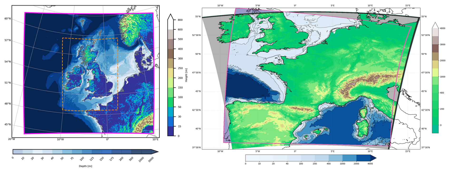
Figure 1 The domains of the two systems. Left: The UKC4 domain used for the UM, NEMO and WWIII components. The land model orography and ocean model bathymetry are also shown. The magenta box covers the outer domain, while the orange dashed area shows the extent of the regular 1.5×1.5 km inner region of UM. Right: The AROBASE (AROME-NEMO) regional forecast system over Metropolitan France, illustrated by AROME orography (colours, in m) over the 1.3 km resolution Lambert Conformal grid and by NEMO bathymetry (blue colours with contours, in m). The pink box/purple areas show the whole extension of the FRA36 ORCA grid. The black zone corresponds to the AROME extension zone (E-zone). The grey zones correspond to uncoupled sea areas for AROME.

2.1.1 UM Regional Atmospheric and Land Component

The atmospheric component of UKC4 (the Unified Model, UM version 13.5) is implicitly coupled with the Joint UK Land Environment Simulator (JULES) for land surface and river routing processes. The regional atmosphere and land configuration is RAL3.3 (Bush et al., 2025). Compared to its predecessors, RAL1 and RAL2 (Bush et al., 2020, 2023), RAL3.3 introduces several key improvements, including an enhanced representation of cloud and precipitation processes through a double-moment microphysics scheme. Additionally, a bi-modal cloud scheme improves cloud cover realism, while refinements in the boundary layer parameterisation enhance the representation of turbulent mixing. The SOCRATES radiative transfer scheme (Edwards and Slingo, 1996; Manners et al., 2018), configured as in Global Atmopshere 3.1 (Walters et al., 2011), computes shortwave (SW) and longwave (LW) radiation in six and nine spectral bands, respectively. It provides atmospheric temperature increments for updating prognosed temperatures and surface fluxes, and derives model diagnostic fluxes.

The domain is a rotated pole curvilinear grid with variable-resolution, with horizontal grid lengths ranging from 1.5 in the central domain (orange dashed line in Fig. 1 left) to 4.4 km in the outer domain, named UKV domain (Tang et al., 2013). In the vertical, the domain is distributed in 70 vertical levels, with model top around 40 km. These resolutions enable an explicit representation of convective processes: deep and shallow convection are explicitly resolved by the model dynamical core (Bush et al., 2025). A timestep of 60 s is used.

2.1.2 NEMO Regional Oceanic Component

The ocean component uses the Atlantic Margin Model 1.5 km domain (AMM15) with the Coastal Ocean 8 (CO8) configuration (Graham et al., 2018; Tonani et al., 2019) and employs NEMO version 4.0.4 on a 1.5 km resolution on a curvilinear grid with the same rotated pole as the atmosphere. The vertical discretisation consists of 51 hybrid z-s levels, which means fixed depth levels in the deeper part of the domain, and terrain-following levels in the shallower part, with a transition zone on the shelf-break. The 1 m constant surface thickness guarantees uniform surface heat fluxes. The model incorporates a non-linear free surface formulation and an energy-conserving momentum advection scheme. Lateral boundary conditions are prescribed using a free-slip approach (Tonani et al., 2019).

Tidal forcing of Finite Element Solution-2014 (FES2014) is implemented using 11 tidal constituents (M2, S2, N2, K1, O1, Q1, M4, K2, P1, MS4, MN4), applied via a Flather radiation boundary condition (Flather, 1976), and further refined by incorporating an equilibrium tide representation. Heat and fluxes are provided directly by the regional atmospheric model. Mass, momentum, and energy exchanges between the atmosphere and the underlying land and ocean surfaces are modeled using the community land surface scheme JULES (Best et al., 2011; Clark et al., 2011). Heat fluxes are passed directly to the ocean, while 10 m neutral winds are passed to the wave model, which calculates the momentum flux and sends it to the ocean. In this study, NEMO uses a baroclinic time step of 60 s, with the barotropic time step set to one-thirtieth of that value. The AMM15 model has two unstructured lateral boundaries to the north, west, and south with the Atlantic Ocean, and to the east with the Baltic Sea, provided by Copernicus Marine (CMEMS) models. The Atlantic boundary comes from global Marine Forecasting Centre (GLO-MFC) global ocean model PSY4 which is based on NEMO ORCA12, which supplies hourly Sea Surface Height (SSH), daily mean temperature and salinity at all depths, and daily barotropic velocity. The Baltic boundary uses data from BAL-MFC, also based on NEMO, providing hourly temperature, salinity, and barotropic velocity. Rivers use climatological values, as described in Tonani et al. (2019).

The configuration ensures consistency with the atmospheric component by overlapping its higher-resolution inner domain with that of the UM. A timestep of 60 s is used.

2.1.3 WAVEWATCH III Regional Wave Component

The wave component is based on WAVEWATCH III (WWIII) version 7.13, which has been modified to support coupling exchanges (Lewis et al., 2019). The model domain covers the northwest European shelf, employing a two-tier Spherical Multiple-Cell grid refinement. In the open ocean, grid resolution is approximately 3 km, whereas in coastal regions where the water depth is less than 40 m, resolution increases to 1.5 km to better capture nearshore processes. The timestep for WWIII is 600 s.

Wave dynamics are parameterised using the ST4 package (Ardhuin et al., 2010), which accounts for wind-wave interactions, whitecapping dissipation, and swell attenuation. To further refine wave behavior in shallow waters, the model includes the surf-breaking parameterisation proposed by Battjes and Janssen (1978) and applies the JONSWAP bottom friction formulation (Hasselmann et al., 1973) to represent wave energy dissipation due to seabed interactions. These parameterisations ensure that the UKC4-Wave configuration is well-suited for intermediate and shallow water environments, such as those characteristic of the northwest European shelf.

2.2 Coupling and Forecast Set Ups for UKC4

Coupling between these components is achieved through the Ocean-Atmosphere-Sea Ice-Soil (OASIS-MCT) coupler (Valcke et al., 2015). The atmosphere sends 10 m neutral winds to the wave model and pressure and heat fluxes to the ocean model. The waves then send the surface stress, significant wave height and mean period and Stokes drift to the ocean. The ocean feeds back the temperature and currents to the atmosphere, and the currents and total water depth to the waves. The model is configured with a 10-min coupling frequency to capture high-frequency events such as meteotsunamis, as the standard 1-h coupling interval was previously found to be insufficient (Berthou et al., 2026). Instantaneous Mean Sea Level Pressure (MSLP) is output from the UM and is interpolated by the OASIS coupler onto the 1.5 km NEMO grid using bi-linear interpolation weights computed with the Earth System Modelling Framework (ESMF) library. In this article, we use the UKC4 in two modes: (i) 3-d hindcast started at 00:00 UTC 17 June 2022, with atmosphere and ocean Lateral Boundaries (LBCs) reset to day 1 global forecasts every day, (ii) 5-d ensemble forecasts started 00:00 UTC 17 June 2022 and 15 June 2022, with atmospheric LBCs coming from MOGREPS-G global forecasts, and deterministic ocean LBCs from GLO-MFC and BAL-MFC for the Atlantic Ocean and Baltic Sea boundaries respectively. The ensemble setup consists of the 18-member Ensemble-RCS framework, which integrates the atmosphere ensemble forecast system MOGREPS-UK (Hagelin et al., 2017) with the regional atmosphere-ocean-wave system. It includes one unperturbed reference simulation and 17 perturbed members, where atmospheric initial and lateral boundary conditions are generated by downscaling perturbations from the global MOGREPS-G system. While the atmospheric component is ensemble-based, the ocean and wave components are deterministic, with coupling handled consistently across all members; further technical detail is available in Gentile et al. (2022).

2.3 Météo-France Coupled System: AROBASE

The AROBASE coupled system is an updated version of the AROME-NEMO system described by Pianezze et al. (2022), but with a smaller regional extension.

2.3.1 AROME Regional Atmospheric Component

The atmospheric model is the non-hydrostatic AROME NWP regional model (Seity et al., 2011; Brousseau et al., 2016) at version cy46t1. The AROME configuration used here is similar to the one used operationally at Météo-France. In more detail, AROME has 1429×1525 physical horizontal grid points with a 1.3 km resolution, plus an extension zone to solve spectral fields with a width of 11 points at the Northern and Eastern boundaries of the domain (black bands in Fig. 1). The vertical grid has 90 hybrid η levels with a first-level thickness of almost 5 m. The advection scheme in AROME is semi-Lagrangian, and the temporal scheme is semi-implicit with a time step of 50 s. The 1.5-order turbulent kinetic energy scheme from Cuxart et al. (2000) is used, with the additional current feedback effect (CFB) taken into account in the tri-diagonal problem associated with the discretisation of the vertical turbulent viscosity (Renault et al., 2019; Bouin and Lebeaupin Brossier, 2020; Pianezze et al., 2022).

The deep convection is explicitly resolved while the shallow convection is parameterised with the eddy diffusion Kain–Fritsch (EDKF) scheme (Kain and Fritsch, 1990). The ICE3 one-moment microphysical scheme of Pinty and Jabouille (1998) is used to compute the evolution of five hydrometeor species (rain, snow, graupel, cloud ice and cloud liquid water). Radiative transfer is based on the Fouquart and Bonnel (1980) scheme for short-wave radiation and the Rapid Radiative Transfer Model (RRTM) for long-wave radiation (Mlawer et al., 1997). The surface exchanges are computed by the SURFace EXternalisé (SURFEX) surface model (Masson et al., 2013) considering four different surface types: land, towns, sea and inland waters (lakes and rivers). Output fluxes are weight-averaged inside each grid box according to the fraction of each respective tile, before being provided to the atmospheric model at every time step. Exchanges over land are computed using the ISBA (interactions between soil, biosphere and atmosphere) parameterisation (Noilhan and Planton, 1989). The formulation from Charnock (1955) is used for inland waters, whereas the town energy balance (TEB) scheme is activated over urban surfaces (Masson, 2000). For the sea surface, the albedo is computed following the Taylor et al. (1996) scheme, and sea surface fluxes are computed with the ECUMEv6 parametrisation (Roehrig et al., 2020; Bouin and Lebeaupin Brossier, 2020).

2.3.2 NEMO FRA36 Regional Oceanic Component

The oceanic model is based on version 4.2 of NEMO (Madec et al., 2023). The regional configuration, named FRA36, is a sub-domain of the eNEATL36 grid (Pianezze et al., 2022). The horizontal grid has 802×937 grid points over an ORCA projection with a 1/36° resolution (corresponding to a resolution between 1.8 km in the North Sea and 2.4 km South of the Balearic Islands). The vertical grid contains 50 stretched z-levels with level thickness between 0.5 m at surface and around 450 m for the deepest level (i.e. at 5700 m depth). In Fig. 1, the pink box marks out the full FRA36 grid, but for some parts inside corresponding to purple or grey zones, FRA36 does not resolve the ocean (and no bathymetry is defined). The temporal scheme for both tracers and momentum is a leapfrog scheme associated with a Robert–Asselin filter to prevent model instabilities (Leclair and Madec, 2009). The free surface is explicit with time splitting, with a baroclinic time step of 150 s and a barotropic time step 30 times smaller. Physical and numerical parameterisations are based on the operational Iberia-Biscay-Ireland (IBI) configuration (Levier et al., 2021) of the Copernicus Marine Service (CMEMS).

FRA36 has five open lateral boundaries with rim size of 10 points: one western boundary between southern Ireland and Galicia in Spain; one southern boundary between the Valencia region in Spain and the western cap of Sicily; one eastern boundary in the Tyrrhenian Sea; and two northern boundaries: one in the Irish Sea and one between southern Scotland and the northwestern coast of Germany (near Denmark). Open boundary conditions (OBCs) are based on the 2D characteristic method (Blayo and Debreu, 2005). The atmospheric pressure component is added, hypothesising pure isostatic response at open boundaries (inverse barometer approximation). River freshwater inputs are imposed partly as daily climatological OBC in the domain locations for 17 main rivers and partly as a climatological coastal runoff to close the water budget from land. The tidal forcing is prescribed from the FES2014 dataset (Carrere et al., 2015) and applied as an unstructured boundary in the NEMO domain: the main 11 tidal harmonics (M2, S2, N2, K1, O1, Q1, M4, K2, P1, Mf, Mm) are used. Solar penetration is parameterised according to a five-band exponential scheme (considering the UV radiations) function of surface chlorophyll concentrations, using monthly climatological 2D fields as in IBI.

2.3.3 Coupling and Forecast Setups for AROBASE

Communications between AROME and NEMO models are performed with the coupling interface built between SURFEX and the Ocean–Atmosphere–Sea Ice–Soil coupler (OASIS3-MCT_5.0, Craig et al., 2017; Valcke et al., 2021), as described in Voldoire et al. (2017). Instantaneous Mean Sea Level Pressure (MSPL) is sent from AROME through OASIS, which is used by NEMO using bi-linear interpolation computed with the Spherical Coordinate Remapping and Interpolation Package (SCRIP) inside OASIS. During the coupled simulation, AROME/SURFEX sends the net non-solar heat flux, the two components of the wind stress and the net freshwater flux computed for the sea tile only to NEMO, and they are then imposed at the surface boundary condition of NEMO. The solar heat flux is also sent to NEMO and is used to calculate the penetrative radiation in the ocean. The atmospheric surface pressure is also exchanged interactively during the coupled simulation for the inverse barometer approximation. In return, NEMO sends the sea surface temperature and the sea surface current components to AROME/SURFEX. For all the exchanged fields, the coupling frequency is 600 s and the interpolation method is bilinear. Where the AROME sea domain is masked for coupling (grey areas in Fig. 1), AROME uses a SST constant in time and equal to the one used at the initial time, and the surface currents taken are always equal to zero there.

The AROBASE forecast starts at 00:00 UTC 17 June 2022 and has a duration of 72 h. AROME is run here without data assimilation, but, like when run operationally, AROME is initialized with the AROME-3dvarfr analyses. It is forced at its lateral boundaries by the operational global hourly forecast from ARPEGE (Courtier et al., 1991) that started on 00:00 UTC 17 June 2022. SURFEX is initialized over continental surfaces and over the uncoupled ocean areas (grey zones in Fig. 1) with the AROME-3dvarfr surface analysis.

FRA36 is initialized by instantaneous fields issued from the restart of an hindcast ocean-only run that started at 00:00 UTC 1 June 2022. It is forced at the OBC by daily-averaged forecasts of temperature, salinity, horizontal currents and SSH from the global CMEMS configuration at $\mathrm{1}/\mathrm{12}$°.

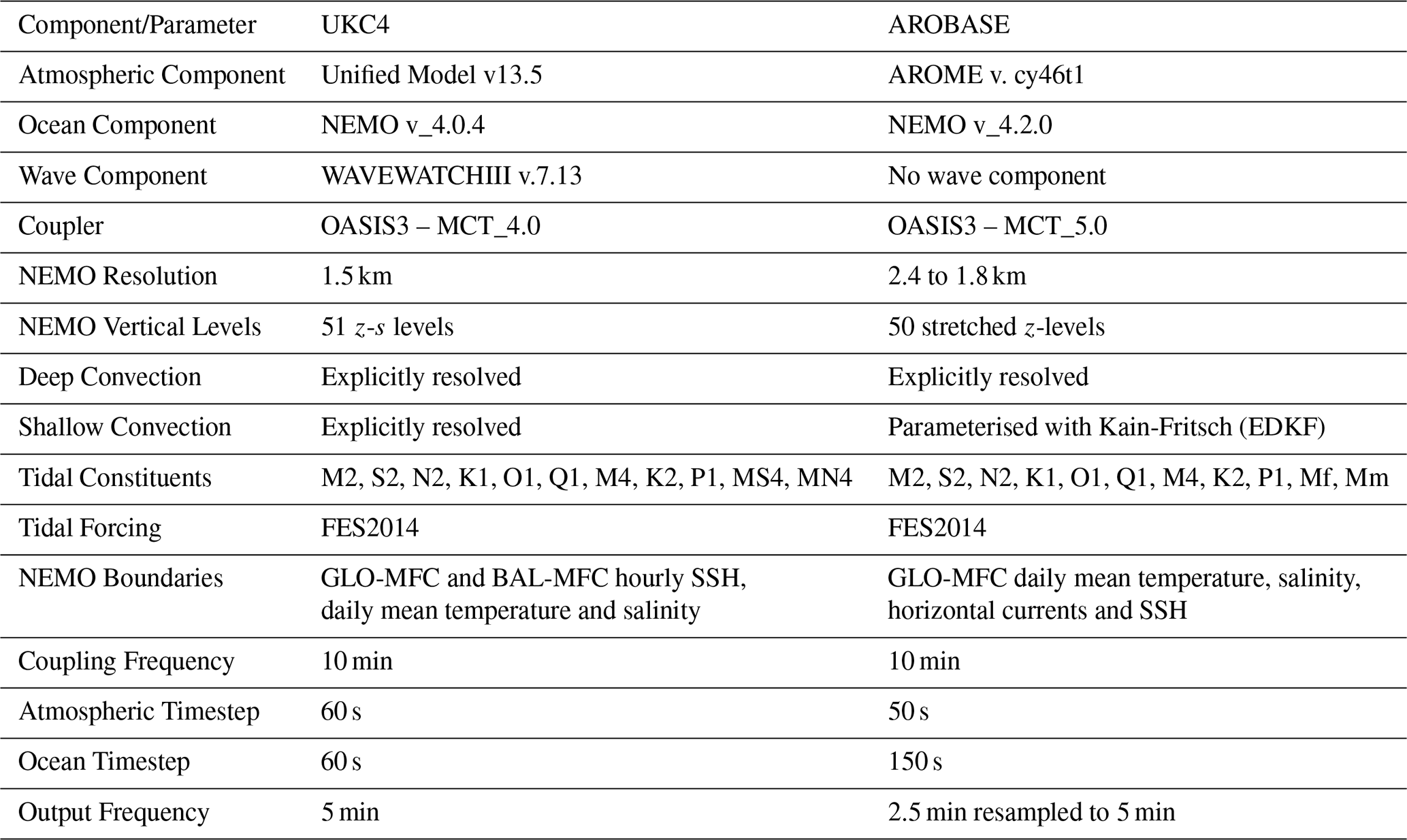
Table 1 Comparison of key configuration aspects of the UKC4 and AROBASE models.

2.4 Tide Gauge Data

To validate the results of the model outputs, we use data from a number of tide gauges around the UK, Ireland, and France, which measure sea level variations over time. The data for the locations for Ireland (Wexford, Ballycotton, Union Hall, Castletownbere) and France (Dieppe, Le Havre, Brest, Le Crouesty, Les Sables d'Olonne) are as described in Renzi et al. (2023). For the UK, sea level data are taken from the UK National Tide Gauge Network (NOC, 2025). The locations of all stations used in this study can be seen in Fig. 2.

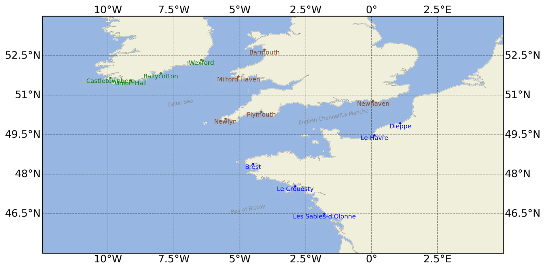
Figure 2 Locations of tide gauges used in the analysis. Colours indicate the country responsible for maintaining each station: green for Ireland, brown for the United Kingdom, and blue for France. Irish stations record at 5-min intervals, UK stations at 15 min intervals, and French stations record at either 5 or 1 min intervals.

3 Methods

This analysis focuses on the meteotsunami event of 18 June 2022, previously examined by Renzi et al. (2023), to validate model outputs against in situ tide gauge observations and evaluate model accuracy. Only the 10-min coupling configuration is presented for both systems, as the 1-h coupling was shown to be insufficient for capturing meteotsunamis, a limitation discussed in detail by Berthou et al. (2026) and confirmed in this case study. To better capture the meteotsunami signal, we use a 5-min output frequency for both UKC4 and AROBASE, aligning with the typical 5-min resolution of most observational datasets. Observational data, however, were retained at their original sampling rates to preserve the highest level of detail in the signal. The analysis is based on filtered SSH to isolate the meteotsunami signal, as shown in Figs. 3, 4, and 5, which correspond to observation sites in the UK, Ireland, and France, respectively.

To extract the meteotsunami signal, a high-pass Butterworth filter is applied. This signal processing technique suppresses low-frequency components while retaining high-frequency variations characteristic of meteotsunamis. The filter is implemented as follows:

$$\begin{array}{}\text{(1)}& H\left(s\right)={\displaystyle \frac{s^n}{s^n+{\mathit{\omega }}_{\mathrm{c}}^n}}\end{array}$$

where H(s) is the transfer function, s the complex frequency variable, ω_c the cutoff frequency, and n the order of the filter.

Specifically, a 5th-order high-pass Butterworth filter is used, with a 1.5-h cutoff for filtering both sea surface height (SSH) and mean sea level pressure (MSLP). These filtering parameters effectively remove low-frequency background variations while preserving the key high-frequency components of meteotsunami-related atmospheric and oceanic disturbances, which typically range between 10 and 60 min.

For SSH, low-frequency variations primarily stem from tidal and subtidal influences, which have characteristic periods exceeding 12 h. In contrast, for MSLP, the filtered low-frequency components correspond to large-scale atmospheric systems, such as synoptic weather patterns. By applying this filtering approach, we retain short-period atmospheric pressure disturbances, including gravity waves and squall lines, which are known to play a crucial role in meteotsunami generation.

The coupled simulations were started one day before the event on 17 June and ran for three days, driven by analysed global fields at their lateral boundary conditions. The filter is applied on the whole three days of the simulation.

4 Analysis of the 18 June 2022 Meteotsunami Event

4.1 Sea Surface Height Signal

The event of 18 June 2022 triggered multiple meteotsunamis across the UK, Ireland, and France (Renzi et al., 2023; Sibley, 2022; McCarthy and Berry, 2022). In this section, we compare model outputs to observations from tide gauges that recorded a clear meteotsunami signal. The analysis focused exclusively on the filtered sea surface height (SSH) to isolate the meteotsunami component at locations in the Celtic Sea (Fig. 3), the English Channel (Fig. 4), and the Bay of Biscay (Fig. 5). All plots use consistent axis ranges to ensure comparability across locations and to allow signals at sites with weaker amplitudes to remain visible. As a result, for locations with stronger signals, such as Union Hall and Milford Haven, the full range is not entirely displayed. To address this, the complete signal for these two sites is provided in the Appendix (Fig. A1). It is important to note that, at most locations, the tide gauge data were received from the Sea Level Station Monitoring Facility (https://www.ioc-sealevelmonitoring.org/, last access: 7 July 2026) before quality control procedures, retaining the extreme values. However, at some sites, primarily in the UK, the quality controlled datasets excluded these extremes, and therefore raw data (Channel 2) were used to ensure that the meteotsunami signal was preserved.

The meteotsunami signal originated in the Celtic Sea around 09:00 UTC, first reaching Irish locations and then Welsh ones (Fig. 3). It then propagated inside the English Channel from west (Newlyn at 14:00 UTC) to east (Dieppe & Newhaven, 16:00 UTC) (Fig. 4). Along the western French coast, the signal was first observed in Brest at around 15:00 UTC, and reached the Bay of Biscay by 17:00 UTC (Fig. 5). The event persisted for about 12 h in the Celtic Sea (Ireland and Wales), and between 18 and 24 h at locations in the English Channel and southwestern France. The highest recorded amplitudes reached 1.0 m in Union Hall (Ireland) and 0.9 m in Dieppe (France). Both systems reproduced the event’s timing and duration reasonably well, although a delay of a few hours was observed in the Channel. They generally underestimated the amplitude of the event, in particular AROBASE. However, the UKC4 system captured the highest amplitudes in Milford Haven (up to 0.9 m), though modeled values remain around 0.2 m at other gauges.

Focusing on the Celtic Sea region (Fig. 3), particularly the four Irish tide gauges, UKC4 successfully reproduced the 0.2 m meteotsunami observed in Wexford, with accurate timing and duration, and a modest overestimation of approximately 15 %. At locations where the signal exceeded 0.2 m, the coupled system maintained good agreement in timing and duration, but systematically underestimated amplitude, with a mean underestimation of around 35 %. Model performance is strongest at Ballycotton, while in Castletownbere the signal is weaker but still detectable. Similarly, UKC4 performed well for Welsh locations (Fig. 3), closely matching observations at Barmouth. At Milford Haven, however, the coupled system overestimated the signal by around 30 %. To assess whether the mismatch between the 15-min sampling interval of the observations and the 5-min output of the model contributes to the overestimation, we resampled the model output to 15-min intervals to match the observations (Fig. A2). This resampling resulted in a slight attenuation of the signal; however, the overestimation by UKC4 remains clearly evident. In terms of timing, all locations show a small early arrival in the model predictions, typically by a few minutes.

In contrast, the AROME-France system captured a weak signal (0.03–0.04 m) in Wexford and Union Hall but failed to detect any significant activity in Castletownbere and Ballycotton. This is likely due to Ireland's location, particularly its southern coast, being near the edge of the NEMO FRA36 model domain. No clear meteotsunami signal is detected by AROME-France at Welsh stations.

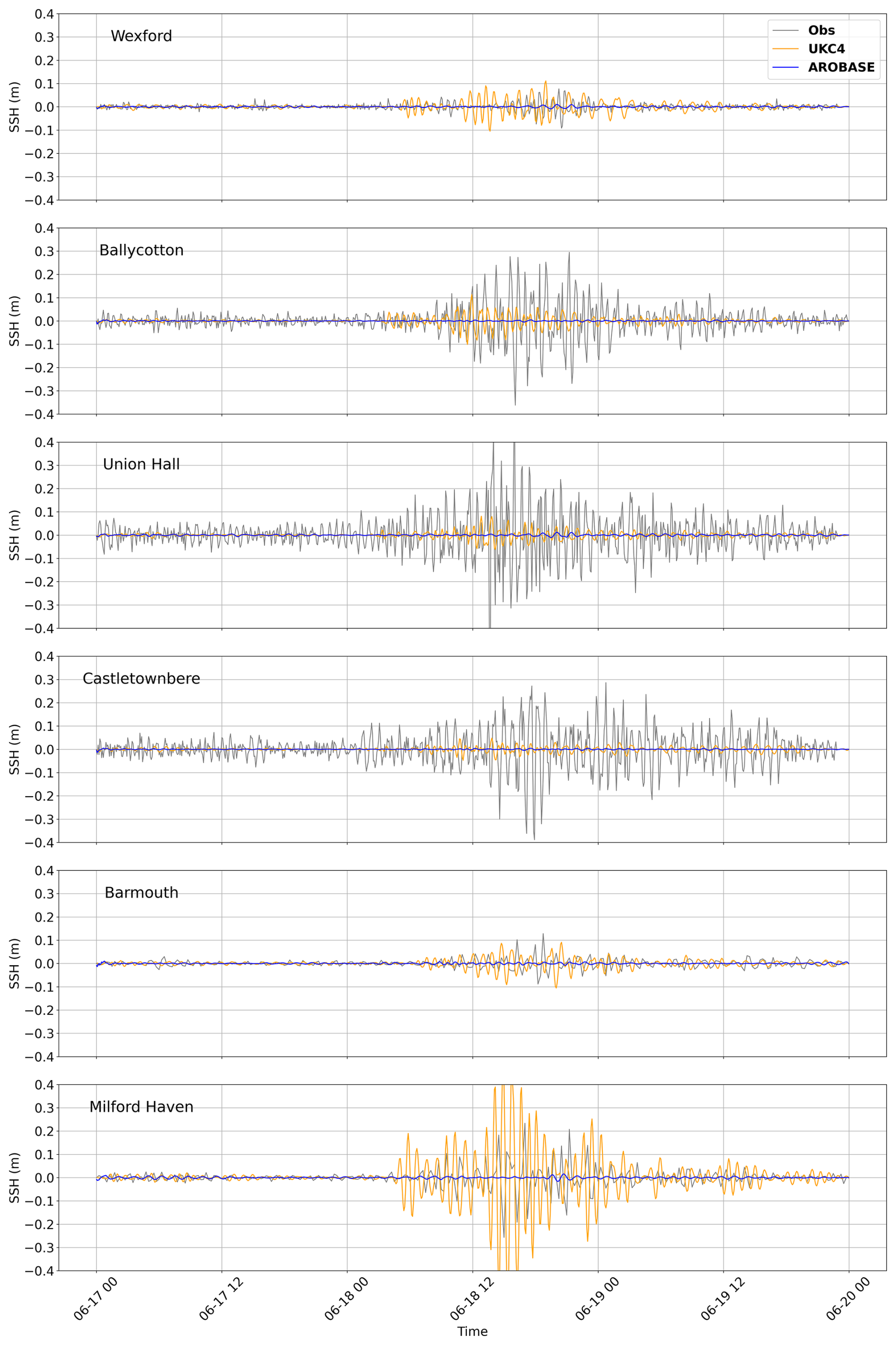
Figure 3 Filtered sea surface height for locations inside and close to the Celtic Sea, ordered West to East. Observations are in black, with 5 min frequency for the Irish stations (top four) and 15 min for the UK stations (bottom two). Models are in orange (UKC4) and blue (AROBASE) and have 5 min sampling frequency. The locations of the observations are shown in Fig. 2.

Focusing on the locations in the English Channel (Fig. 4), the UKC4 system demonstrated good performance in capturing the meteotsunami signal at most UK tide gauge stations (Newlyn, Plymouth, Newhaven). It slightly overestimated the amplitude at Newlyn by approximately 15 %, with a larger overestimation of around 30 % at Plymouth. In contrast, it slightly underestimated the signal at Newhaven by about 10 %. On the French side of the Channel, where tide gauges operate at higher temporal resolution (1–5 min), UKC4 consistently underestimated the meteotsunami signal, with maximum simulated amplitudes remaining below 0.2 m. This corresponds to an average underestimation of about 30 %. In Dieppe, part of this discrepancy may be attributed to the mismatch in sampling frequency between the model output (5-min intervals) and the tide gauge data (1-min intervals). However, at Le Havre, where the observational data also have a 5-min resolution, the model still underestimated observed amplitudes, suggesting broader performance limitations. Despite the amplitude discrepancies, the timing of the modeled signals generally aligns well with observations, with only minor lags of a few minutes at certain locations (most clearly seen in Plymouth).

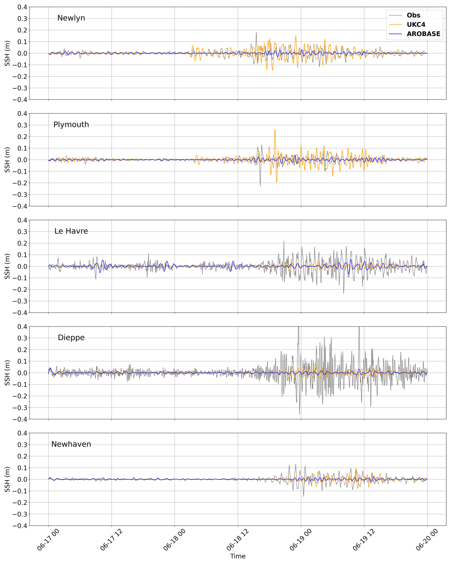
Figure 4 Filtered sea surface height for locations at the edge and inside the English Channel. Observations are in black, with 15 min frequency for the UK stations and 1 min for French stations. Model outputs are in orange (UKC4) and blue (AROBASE) and have 5 min frequency. The locations of the observations are shown in Fig. 2.

The AROBASE system, on the other hand, showed limited ability to reproduce the signal at UK stations. It captured only weak signals at Newlyn and Newhaven but performs somewhat better at Plymouth, where the results are closer to observations. On the French side, AROBASE yields results comparable to UKC4 at Le Havre and, in some instances, showed better temporal agreement with observations. It exhibited an overall amplitude underestimation of about 20 %–25 % at this site. In Dieppe, however, AROBASE underestimated the signal even more than UKC4 for most of the event duration.

Finally, in the Bay of Biscay region along the west coast of France (Fig. 5), both systems were able to capture the meteotsunami signal, although with varying degrees of accuracy. While the overall shape and timing of the signal are reasonably well represented, both systems significantly underestimated the observed amplitudes. AROBASE shows the strongest underestimation, with discrepancies exceeding 60 % at all three locations. UKC4 performs slightly better, but still underestimated the amplitude by approximately 50 %. Despite these amplitude discrepancies, the systems successfully reproduced the timing and duration of the event. However, compared to other regions, the time lag between observed and modeled signals is more pronounced here, reaching 2–3 h, particularly at Le Crouesty and Sables-d’Olonne. This lag suggests a slight delay in the modeled meteotsunami propagation along the French Atlantic coast, possibly due to resolution limitations or inaccuracies in the atmospheric forcing or wave travel paths in this region.

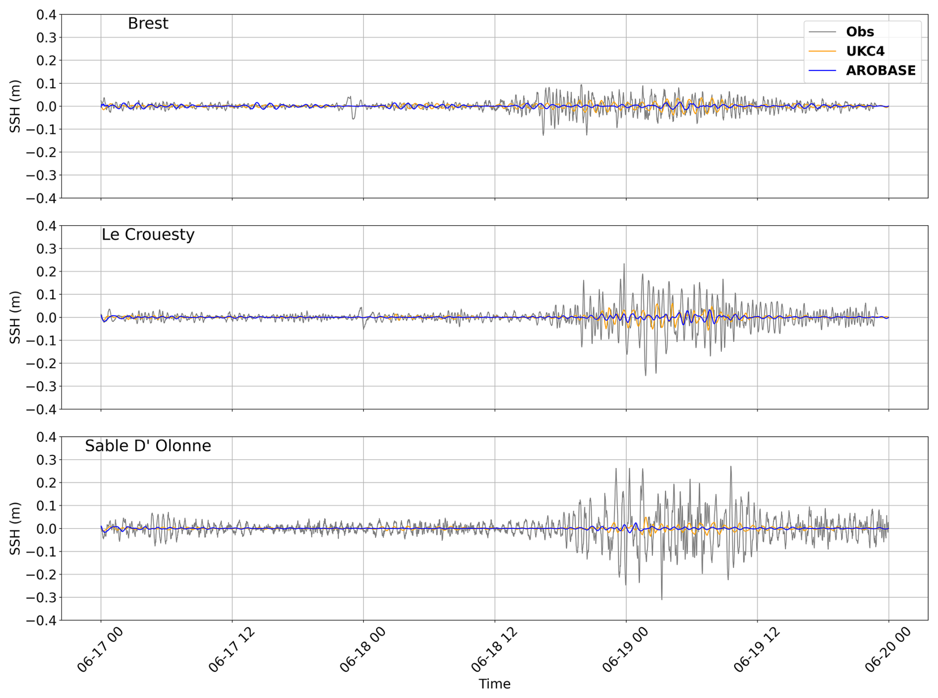
Figure 5 Filtered sea surface height for locations West of France. Observations are in black, with 1 to 5 min frequency. Model outputs are in orange (UKC4) and blue (AROBASE) and have 5 min frequency. The locations of the observations are shown in Fig. 2.

Overall, the UKC4 captured the meteotsunami signal reasonably well, generally underestimating it when amplitudes exceed 0.2–0.3 m, with some exceptions, such as Milford Haven, where it overestimates the signal (30 %).

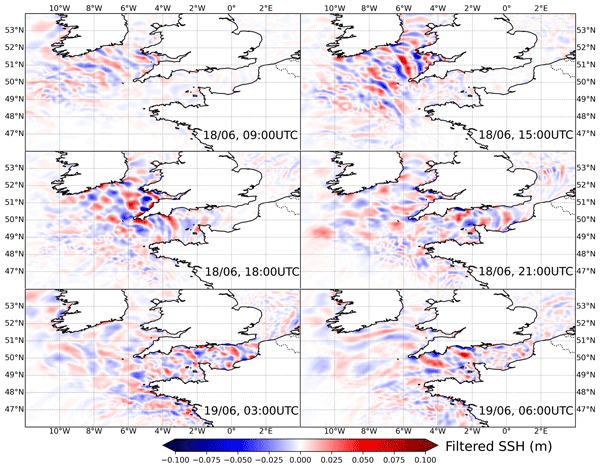
Given the relatively good agreement of the UKC4 system with observations, we now look at the spatial distribution of the meteotsunami signal (Fig. 6). The signal starts at 06:00 UTC around 11° W, 49° N in the Celtic Sea (not shown). At 09:00 UTC 18 June, meteotsunami activity clearly begins in the Celtic Sea near Ireland and the UK: distinct dipole patterns of high and low SSH emerged south of Ireland and around Wales, with a wave length of 45 km, elongated in a northwest/southeast direction. By midday, the activity intensified, reaching parts of Cornwall, with 15:00 UTC marking the peak of the meteotsunami event in these areas. A weaker signal was then observed extending toward the northwestern coast of France, particularly around Brest. It propagated inside the Channel and re-emerges east of the Calais-Dover straight. We note the signal is organised in northwest/southeast bands in the Celtic Sea, but it quickly lost this banded organisation in the English Channel and Bay of Biscay.

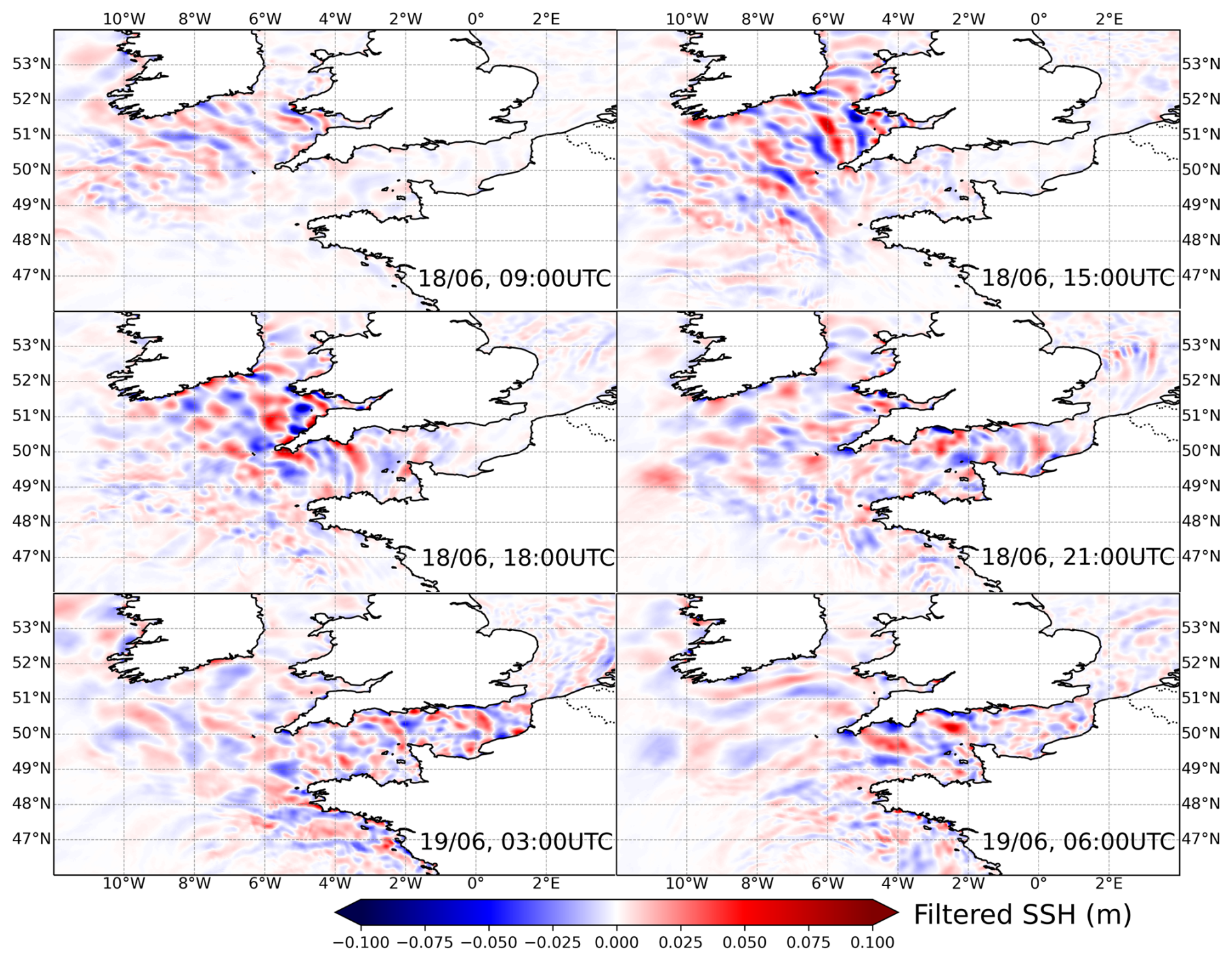
Figure 6 Spatial filtered sea surface height on 18 June at 09:00, 15:00, 18:00, 21:00 UTC and on 19 June at 03:00 and 06:00 UTC.

4.2 Mean Sea Level Pressure Signal Responsible for the Meteotsunami

To understand why UKC4 more accurately predicted the meteotsunami signal compared to the AROBASE system at most locations, the mean sea level pressure (MSLP) patterns captured by each system was analysed. The top panel of Fig. 7 shows the general pattern of MSLP in UKC4, with a low pressure centre North of the UK and one Southwest of France. In between the two systems in the Celtic Sea, sub-mesoscale irregularities can be noted in the isobar patterns, starting at 12:00 (not shown) and developing more strongly at 15:00 and 18:00 UTC. AROBASE started developing them later around 18:00 UTC, both in the Celtic Sea and the Bay of Biscay, where they are more intense for this system (Fig. 7, bottom panel).

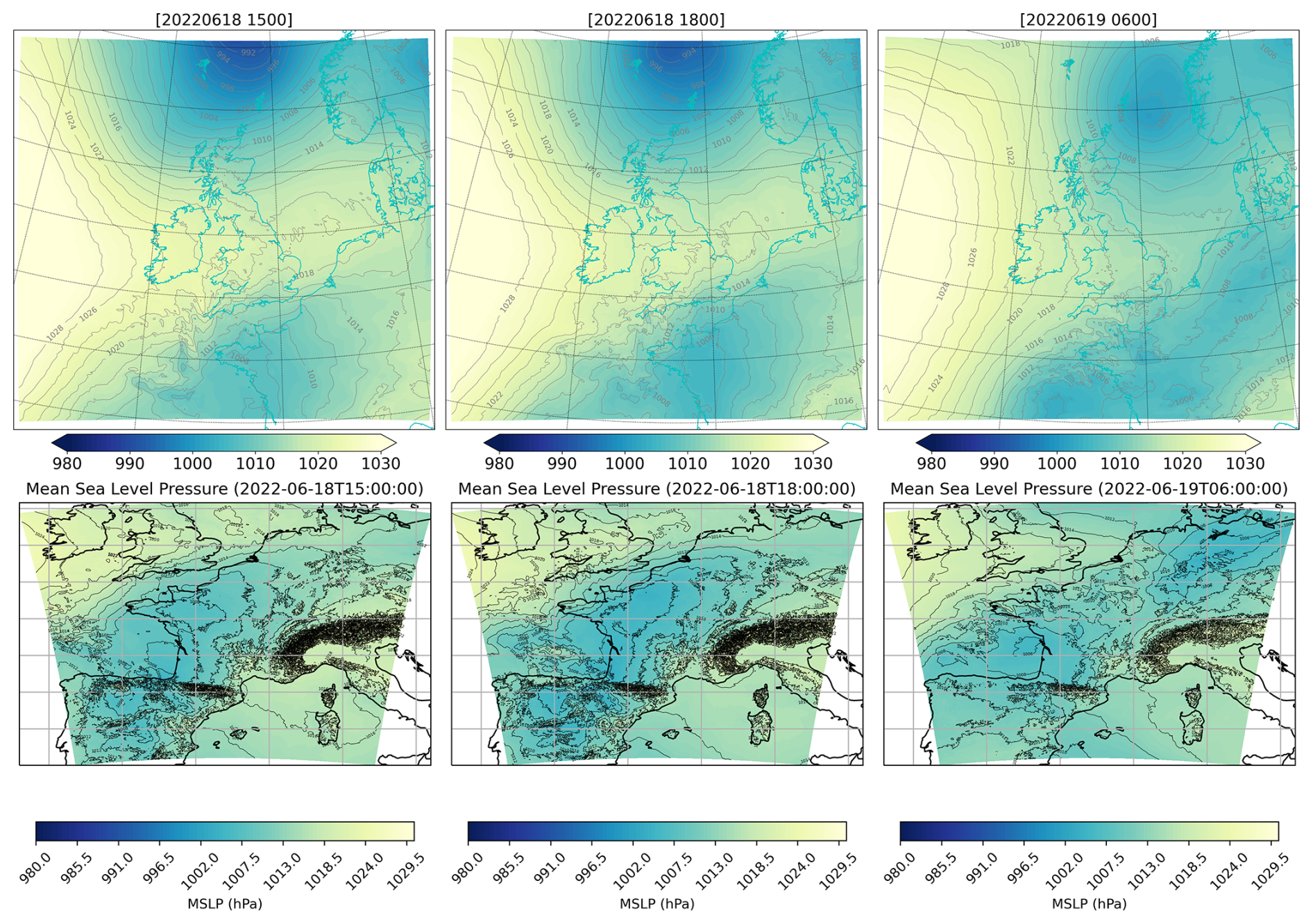
Figure 7 Mean Sea Level Pressure (MSLP) output from the atmospheric component of UKC4 (top) and AROBASE (bottom) for 18 June 2022, at 15:00 (left), 18:00 (center), and 19 June 2022 06:00 (right).

To assess how these atmospheric conditions are transferred to NEMO, the filtered mean sea level pressure (MSLP) output from the OASIS coupler was examined using a 1.5-h cutoff to isolate rapid pressure disturbances. Two open-water locations in the Celtic Sea (50.81° N, 7.04° W; 51.31° N, 5.77° W), two in the English Channel from the lightships near the UK (Channel Lightship – 49.900° N 2.900° W; Greenwich Lightship – 50.4087° N 0.0000° W), and two in the Bay of Biscay close to Le Crouesty (47.38° N, 5.02° W; 47.20° N, 3.49° W) were analysed to highlight differences between the systems. The points are located as stars in Fig. 8. Additionally, two sites in France (near Brest and Le Havre) were included, as their observational data have sufficient temporal resolution to apply the high-pass filter and compare directly with the model output.

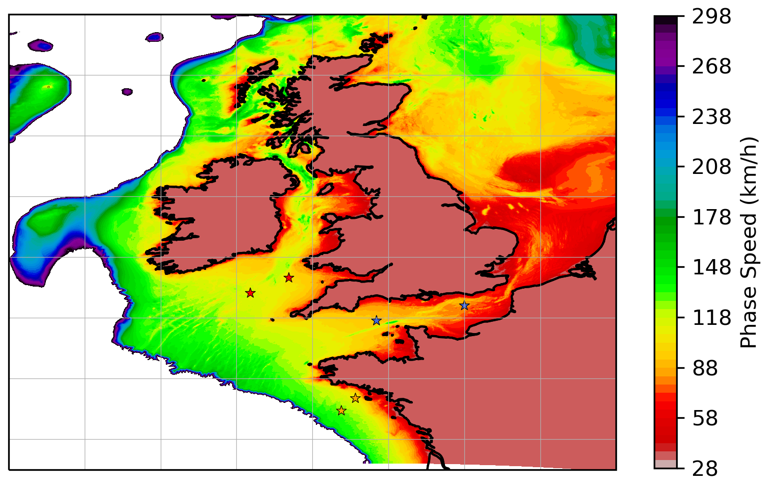
Figure 8 Phase speed for the Northwest European shelf calculated as $\sqrt{gh}$. Colours of the stars indicate the three regions of interest: red for the Celtic Sea, blue for the English Channel, and orange for the Bay of Biscay.

The time series presented in Figs. 9–12 support the spatial patterns discussed earlier. In the Celtic Sea (Fig. 9), UKC4 consistently showed higher disturbance amplitudes than AROBASE, reaching around 200 Pa at two locations. In contrast, the AROBASE system showed weaker disturbances, generally closer to 100 Pa. In both systems, they last for about 8 h. For both systems, the onset of the pressure signal typically occurred around 06:00 UTC, indicating a similar timing of the event.

The results from the lightship locations (Fig. 10) indicated that both systems perform similarly in the Channel, showing a west-east propagation of the high-frequency MSLP perturbation, from 12:00 to 18:00 UTC, consistent with the timing of the meteotsunamis. UKC4 had a stronger amplitude (up to 400 Pa maximum amplitude) than AROBASE in the western part of the Channel, but their amplitude was closer in Greenwich, consistent with the larger meteotsunami amplitude in UKC4 in the Channel. The Figs. 9–12 also revealed an important limitation: because lightship observations are recorded only once per hour, the temporal resolution is insufficient to fully resolve the signal. Consequently, these data offer limited value for detailed analysis and are not included in the plots. This limitation emphasises the need for more frequent recordings, at least every 15 min for MSLP measurements from lightships providing critical data for open-sea locations.

At the two locations in the Bay of Biscay (Fig. 11), the AROBASE system showed a noticeable improvement in capturing high-frequency pressure disturbances, with amplitudes approaching 400 Pa, comparable to those produced by UKC4. In fact, as the forecast progressed, AROBASE occasionally produces greater perturbations than UKC4. This suggests that the finer-scale atmospheric processes were better preserved in AROBASE in this region. However, similar to what was observed in the Celtic Sea, these enhanced pressure fluctuations were not clearly reflected in the SSH signal. Finally, checking the stations where there are observations (Fig. 12), the station locations in France (Brest and Le Havre) exhibit up to 250 Pa disturbances, while both systems showed weaker disturbances, up to 200 Pa, and the disturbances start around 6 h later than the observations. However, both systems performed relatively similarly, with AROBASE having a higher signal in times for Le Havre and UKC4 most of the times for Brest (Figs. 4 and 5).

To further assess the ability of the two models to capture atmospheric perturbations, additional validation of the atmospheric pressure forcing is provided in Appendix Fig. A4. This analysis is based on the same Irish stations used in Renzi et al. (2023), with data processed using consistent filtering. The results corroborate the findings discussed above and offer further insight into why UKC4 outperforms AROBASE. As shown in Fig. A4, UKC4 exhibits very good agreement with the observations, clearly reproducing the 2 hPa pressure jump. Although minor discrepancies in timing are present, the overall representation remains adequate. In contrast, AROBASE shows weaker performance at the two stations within its domain: the pressure jump is less pronounced, which likely contributes to a reduced amplification of the meteotsunami signal.

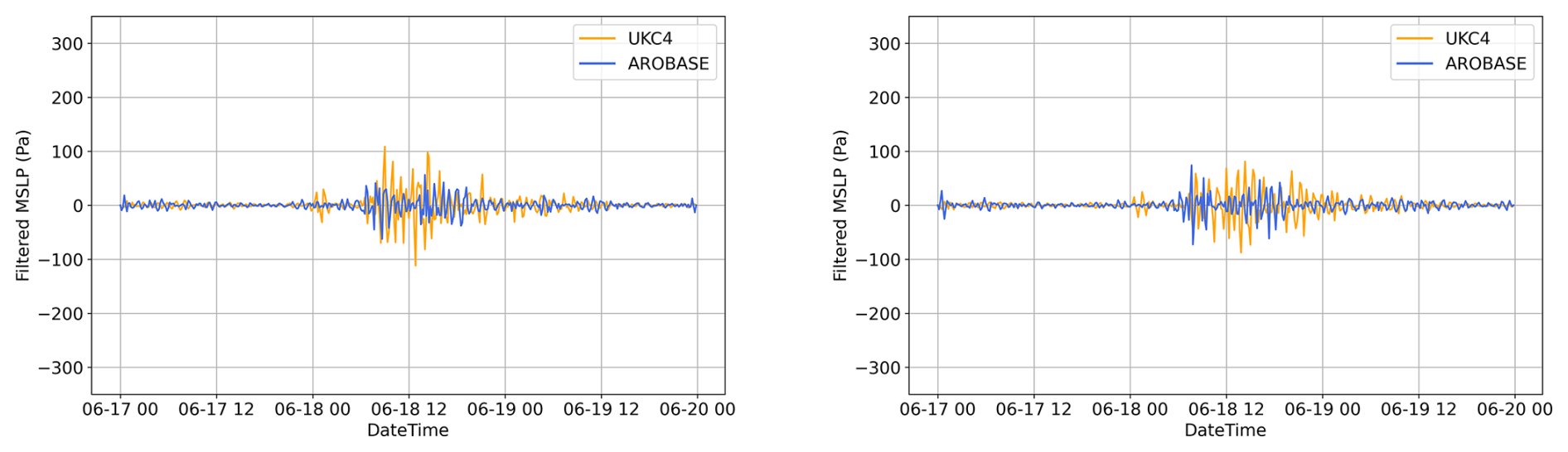
Figure 9 Filtered MSLP time series for the UKC4 (orange) and AROBASE (blue) for the two locations in the Celtic Sea shown as red stars in Fig. 8: 50.81° N, 7.04° W (left panel), 51.31° N, 5.77° W (right panel).

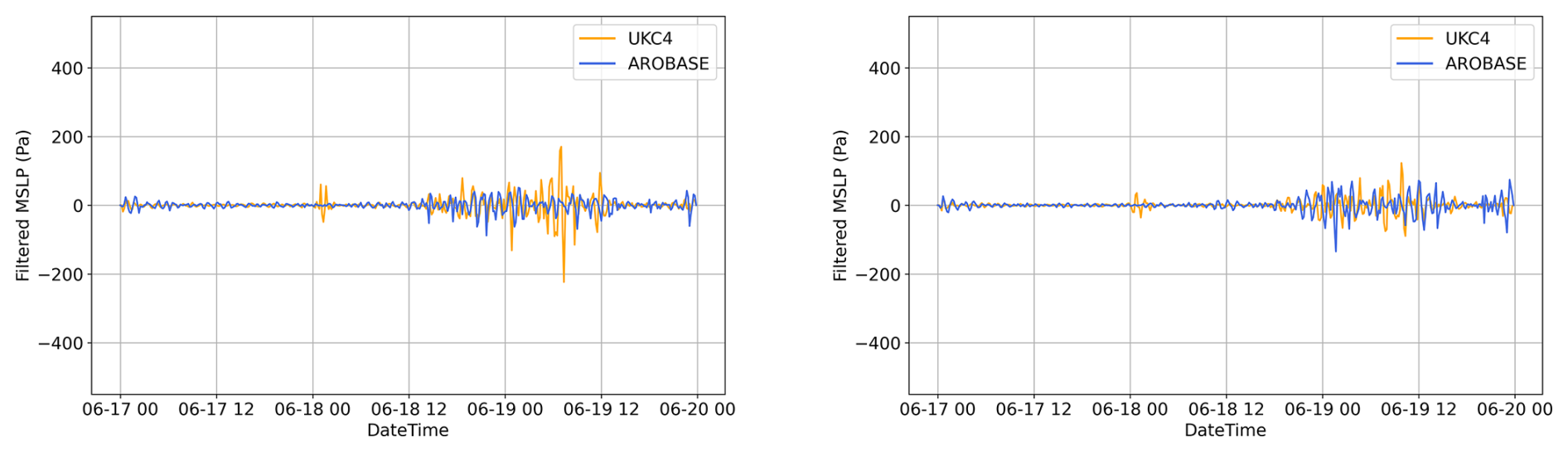
Figure 10 Filtered MSLP time series for UKC4 (orange) and AROBASE (blue) at two lightship locations: Channel (49.900° N, 2.900° W; left panel) and Greenwich (50.4087° N, 0.0000° W; right panel), shown as blue stars in Fig. 8.

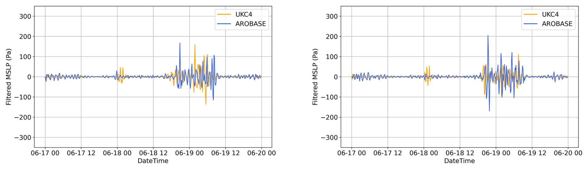
Figure 11 Filtered MSLP time series for the UKC4 (orange) and AROBASE (blue) for the two locations in Bay of Biscay shown as orange stars in Fig 8 (close to Le Crouesty). 46.93° N, 4.04° °W (left panel), 47.34° N, 3.58° W (right panel).

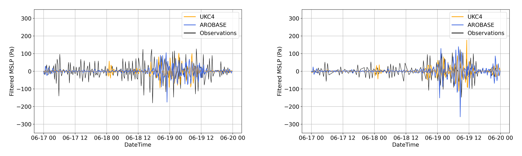
Figure 12 Filtered MSLP time series for the UKC4 (orange) and AROBASE (blue) for the two locations in France: Brest (left panel) and Le Havre (right panel). The black line represents the observations in this locations.

We now examine the occurrence of Proudman resonance in both modeling systems. Propagation speeds were estimated based on lag-correlation analysis of filtered mean sea level pressure (MSLP) perturbations (Fig. 13) using the same station pairs as in Figs. 9–11, whose locations are shown in Fig. 8. For each region, specific time windows were selected to isolate the main part of the event and minimize interference from unrelated disturbances: 18 June 06:00 UTC to 19 June 00:00 UTC for the Celtic Sea, 18 June 10:00 UTC to 19 June 15:00 UTC for the English Channel, and 18 June 20:00 UTC to 19 June 10:00 UTC for the Bay of Biscay. The lag-correlation was then calculated between the filtered timeseries in this time window for each pair of sites and each model.

In the Celtic Sea, UKC4 exhibited a 60-min lag between stations separated by 104.7 km, corresponding to a propagation speed of approximately 104.7 km h⁻¹, aligned with the phase speed characteristic of sea disturbances calculated from the bathymetry of the region (Fig 8). In contrast, AROBASE showed a faster-moving disturbance, covering 104.4 km in 50 min, which corresponded to a speed of 125 km h⁻¹, significantly exceeding the local phase speed (Fig. 8). For the Celtic Sea region, the UKC4 model demonstrated a notably higher cross-correlation between the two points compared to AROBASE, reaching a maximum value of approximately 0.6 at a lag of −60 min. This suggests that the meteotsunami signal in UKC4 maintained both its shape and amplitude during propagation, which likely contributed to its stronger representation of the event. In contrast, AROBASE showed a weaker and more dispersed correlation pattern, indicating potential dissipation or distortion of the signal as it travels.

In the English Channel, UKC4 showed a lag of 180 min over 213.7 km, yielding a speed of 71.2 km h⁻¹, which is again consistent with the local phase speed. AROBASE propagated the signal over 211.6 km in 230 min, resulting in a speed of 55.2 km h⁻¹. While lower, this speed falls within the range of regional phase speeds and may explain AROBASE's relatively better performance near Le Havre, where slower propagation aligns more closely with local conditions. At this location, AROBASE exhibited a higher cross-correlation between the two points (maximum around 0.5 at a lag of −230 min) compared to UKC4, whose maximum correlation was lower and occured at a similar lag.

The Bay of Biscay presented a more complex case due to highly variable bathymetry and corresponding variations in phase speed. For this region, UKC4 exhibited a 100-min lag over a distance of 57.57 km, implying a speed of 34.54 km h⁻¹. AROBASE showed a shorter lag of 40 min for a distance of 58.85 km, giving a speed of 88.28 km h⁻¹. While AROBASE's speed was more consistent with phase speeds in the open ocean, it was not adequately captured the transition toward the coast. UKC4, although slower overall, appeared to better match the required speeds closer to the coastline. Both models, however, exhibited difficulty in this region, suggesting challenges in representing the forcing mechanisms. Note that the points were chosen according to the direction of propagation of the meteotsunami in the UKC4 system, which was possibly not the correct one for the Bay of Biscay, given that the system failed to amplify the meteotsunami signal there. It was likely that a perturbation propagating more parallel to the coast may had better amplified the meteotsunami. For the Bay of Biscay, both systems exhibited generally lower cross-correlation values relative to the other two regions, reflecting the reduced skill of both UKC4 and AROBASE in capturing an organised pressure signal. Nonetheless, UKC4 maintained slightly higher correlation values (maximum ∼0.5 at a lag of −100 min) than AROBASE (maximum ∼0.4 at a lag of −40 min), indicating that the signal's structure is somewhat better preserved in UKC4. The persistently lower correlations for both systems may partially explain their limited success in representing meteotsunami characteristics in this region.

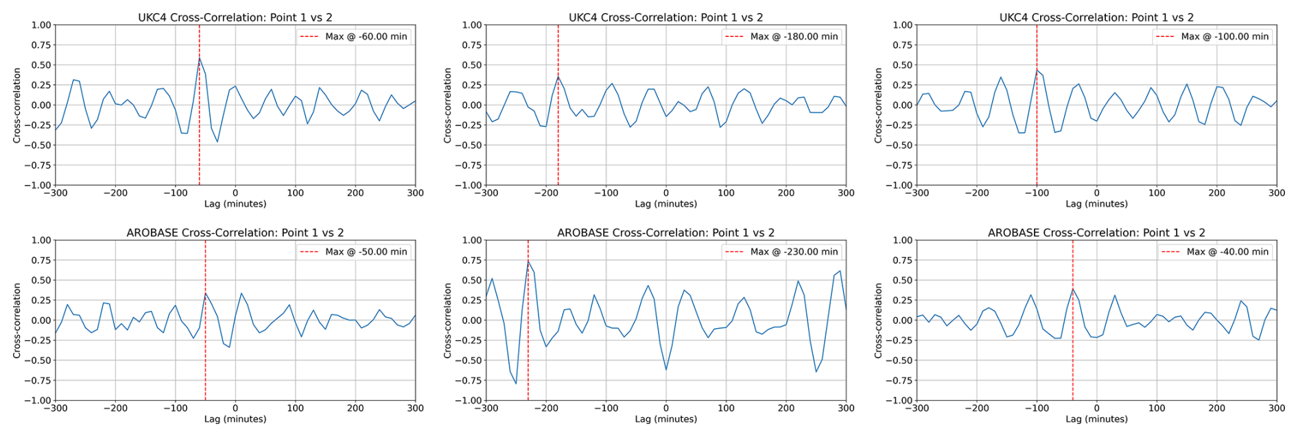
Figure 13 Filtered MSLP cross-correlation of perturbations for UKC4 (top) and AROBASE (bottom) in Celtic sea (left); the Channel (middle); and Bay of Biscay (right). All point are shown in Fig. 8.

We can therefore conclude that the UKC4 system showed larger and slower pressure disturbances in the Celtic Sea, with Proudman resonance at play, leading to a 0.9 m maximum amplitude in the UK. AROBASE, on the other hand, had weaker and faster moving MSLP perturbations, not able to activate Proudman resonance in the Celtic Sea. In the English Channel, both systems had similar MSLP pressure disturbances and speed able to activate Proudman resonance in different parts of the Channel, though the MSLP signal was less coherent. In the bay of Biscay, the systems may not be propagating in the right direction (too perpendicular to the coast). These differences were further reflected in the cross-correlation analysis, where UKC4 generally preserved the coherence of the pressure signal better than AROBASE, especially in the Celtic Sea and Bay of Biscay, and with slower propagation speed, supporting its superior representation of meteotsunami propagation in these regions.

We note that Renzi et al. (2023) identified Proudman resonance as the main resonance mechanism responsible for this event. The meteotsunami signal presented in Fig. 6 is organised in coherent stripes, which do not show particularly strong coastal enhancement, therefore also suggesting Greenspan resonance was not captured by the model.

4.3 Origins of the Mean Sea Level Pressure Signal

We now examine the origin of these sub-mesoscale pressure disturbances using the UKC4 system. As shown from the MSLP plots (Fig. 7, top panel), the synoptic conditions were dominated by a low pressure system to the north of Ireland and Scotland, with a second system developing southwest of France, which are visible also in the geopotential height (Fig. 14). Between the two systems sits an area of higher pressure, with widely spaced isobars and an area of frontal precipitation, with pockets of rainfall intensities higher than 4 mm h⁻¹ (Fig. 14, bottom panel). In this area, isobars were not smooth (Fig. 7), they present high-frequency irregularities: the geopotential height of the 925 hPa level showed that this pressure level is highly distorted in this area, changing height by about 60–80 m in the space of 100 km. Figure 16 shows the three dimensional structure of the frontal area in terms of wet bulb potential temperature (WBPT) with a map at 850 hPa and two cross-front sections at 09:00 and 18:00 UTC. WBPT incorporates both temperature and humidity field and exacerbates air-mass differences in fronts. The air mass contrast was extremely stark, with cold and dry air in the northwest corner (<282 K) meeting warm and dry air in the southeast (>290 K), with a tongue of high relative humidity (RH > 80 %) along the frontal slope and at upper levels in the warm sector. Red warnings (corresponding to the maximum warning level) for extreme heat were in place in France.

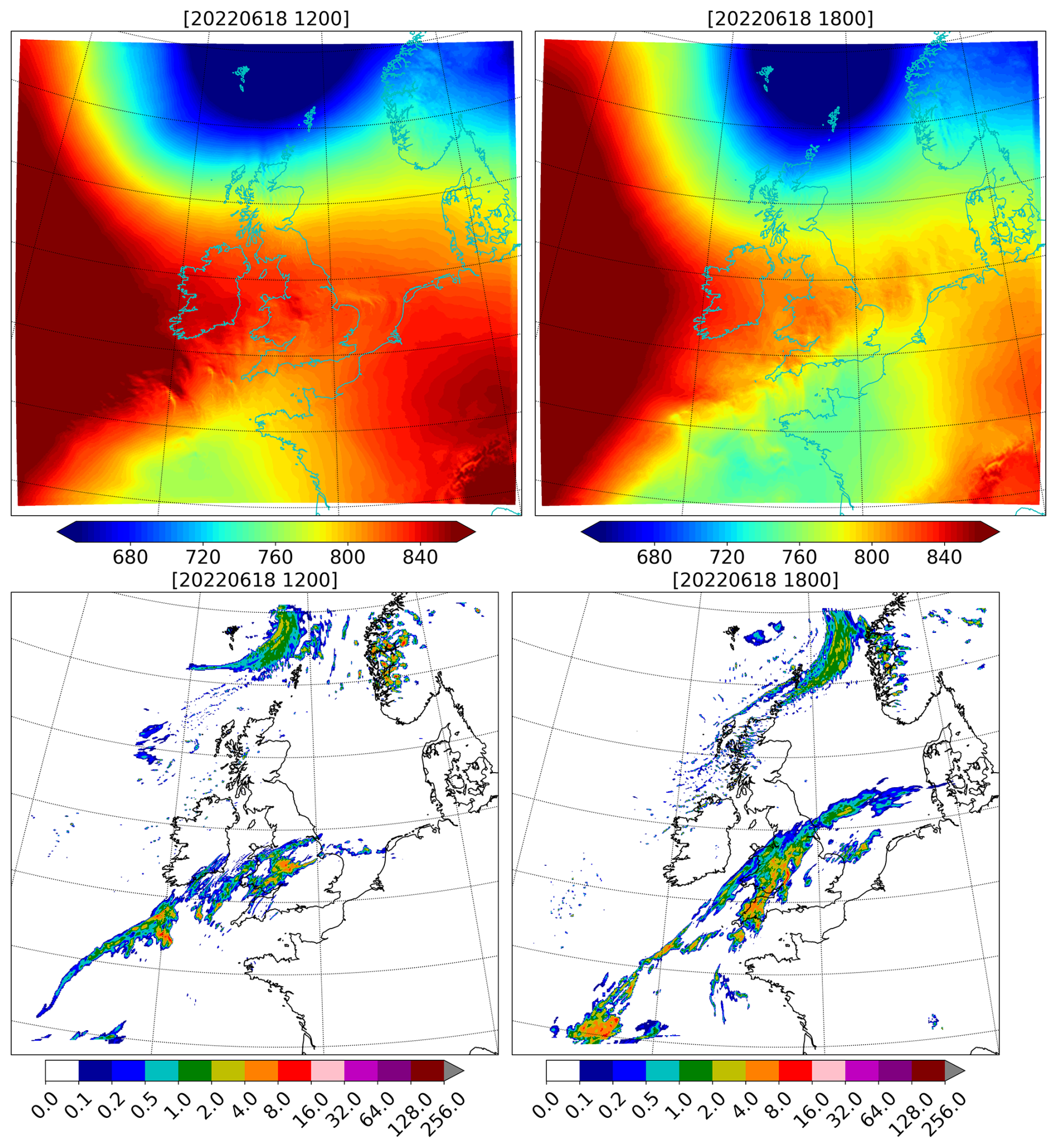
Figure 14 Geopotential height at 925 hPa (m) (top) and precipitation rate (mm h⁻¹) (bottom) for 18 June 2022 at 12:00 UTC (left) and 18:00 UTC (bottom).

Initially, most convective activity was embedded within the frontal surface and a direct thermal circulation with the front was setup (not shown). As time develops convective activity occurred associated with an upper-level warm front (Fig. 15) around 600–700 hPa, which created a distinct separate circulation (Fig. 16a, c). At the same time, the cool air near the surface (possibly combined with a cold pool originating from this upper-level convection) extended ahead of the surface front at 18:00 UTC, creating a moist stable layer (Fig. 16c). The convection from the upper-level front merged with convection initiated by the surface front at 18:00 UTC, as shown by omega contours extending from 300 hPa to the surface. The transition from elevated to surface convection allowed the downdraft to reach the surface. Combining the convective downdraft with the downslope frontal component likely enhances the downdraft and their conjunction was likely generating gravity waves in this near-surface stable layer.

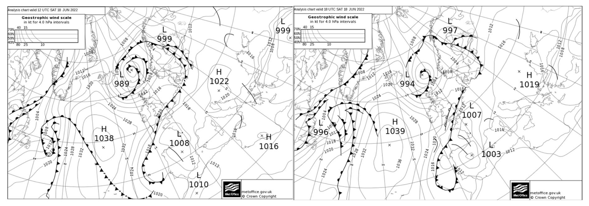
Figure 15 Synoptic conditions for 18 June 12:00 and 18:00 UTC. The upper level warm front is marked on the 18:00 UTC chart (right panel) with empty semi-circles along its line, located over England.

This stable layer was identified in the 850 hPa maps with hatch lines in Figs. 16b, 17a and 18a–b, showing regions with at least 2 K difference between 1000 and 850 hPa levels. It was oriented along the front from southwest to northeast and its width spans 200–300 km. It was initially located in the Celtic Sea at 09:00 UTC, and slowly moved east into the Channel and Bay of Biscay from 18 June 09:00 UTC (Fig. 16b) to 19 June 06:00 UTC (Fig. 18b).

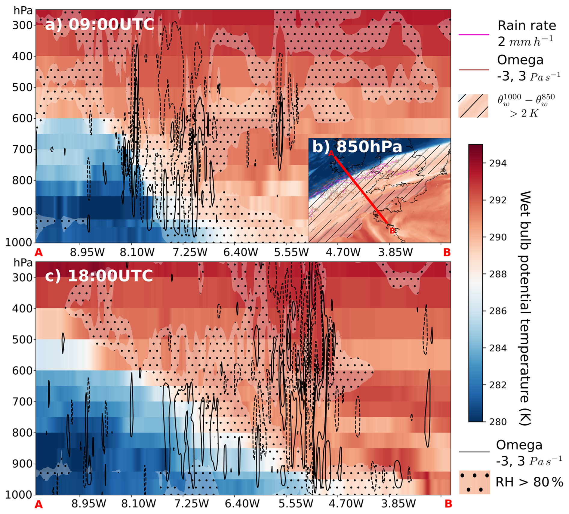
Figure 16 Cross-front cross section of wet-bulb potential temperature (WBPT, colours), isobar vertical velocity (Omega, Pa s⁻¹) in black contours, and relative humidity above 80 % (dotted area) for the 18 June 2022 at 09:00 UTC (a) and 18:00 UTC (c) along the A-B red line in inset (b), which shows WBPT (colours), stable layer ($//$), omega in brown and rain rate in purple.

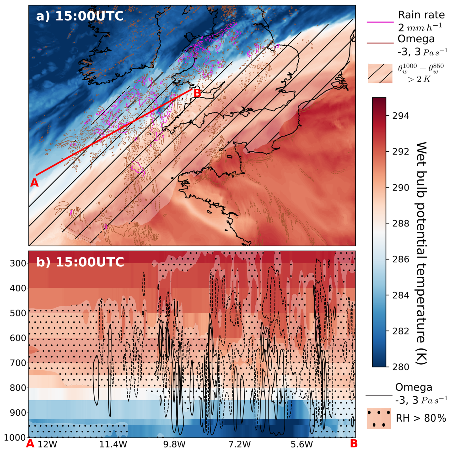
Figure 17 (a) 850 hPa WBPT (colours), stable layer ($//$) where ${\mathit{\theta }}_{\mathrm{w}}^{\mathrm{1000}}-{\mathit{\theta }}_{\mathrm{w}}^{\mathrm{850}}>\mathrm{2}$ K, cross-isobar vertical wind speed (Omega) in brown contour and rain rate contour of 2 mm h⁻¹ in purple for 18 June 2022 at 15:00 UTC. (b) Cross section of WBPT (colours) parallel to front on pressure levels, cross-isobar vertical wind speed (Omega) in black contours (Pa s⁻¹, positive plain, negative dashed), and relative humidity above 80 % (dotted area) along the A-B red line in the Celtic Sea (a).

To understand what happened along this stable layer, we considered along-front cross-section, in the Celtic Sea at 15:00 UTC, when the meteotsunami is at its maximum intensity in UKC4 (Fig. 17). The cool stable layer was once again apparent near the surface. However, there were variations in the height of the cool layer with warmer downdrafts acting to displace the cool air and, via mass continuity, generate waves along the top of the stable layer. There were pulses of downdrafts that rise and fall in height (with possible weaker updrafts in between) acting as a signal for the gravity waves, but also the forcing for the wave generation. These pulses were distinct from the larger and more intense updrafts and downdrafts which were associated with precipitation (pink contours in Fig. 17a), due to convection generated by the leading edge of the cool air mass where lifting at the front of the density current gave rise to convection. Further evidence for the displacement of the cooler air mass as a result of convection was seen in the geopotential height at 925 hPa, which showed that the surface of this pressure level was clearly distorted by this mix of gravity waves and convective up and downdrafts (Fig. 14). This activity started around 09:00 UTC, and becomes more organised at 12:00 UTC. The gravity waves initially propagated in all directions, but they only grow in the southwest/northeast direction, inside the elongated stable layer. By 12:00 UTC (not shown) and 15:00 UTC, these organised patterns emerged and generated the meteotsunami by propagating slowly in the southwest/northeast direction, parallel to the front.

We note the meteotsunami intensity was greatest in Wales in UKC4, whereas in the observations it was most extreme in Ireland. The stable layer may be moving too fast to the east in the modeling system, not allowing the pressure signal to build for long enough on the coast of Ireland. Nevertheless, it is remarkable to see that the modeling system was reproducing a similar intensity of meteotsunamis as observed: a 0.9 m amplitude requires capturing sustained resonant processes, which we are now confident UKC4 can capture. This representation demonstrates that the coupled system successfully captured Proudman resonance in the Celtic Sea: 2 hPa pressure anomalies (Fig. 9) can generate 0.9 m meteotsunamis (Fig. 3).

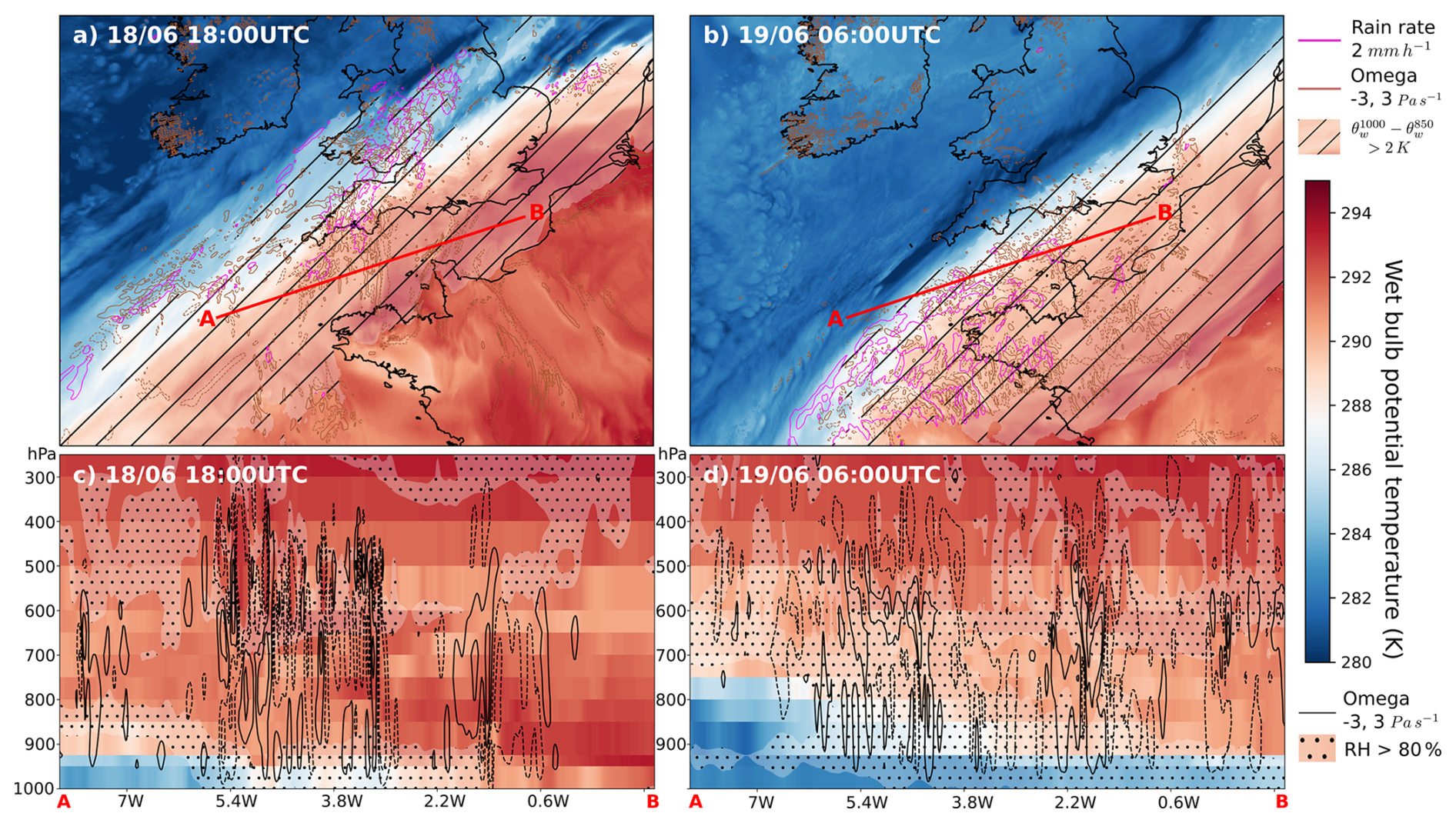
Figure 18 Same as Fig. 17 but for (a, c): 18 June 2022 at 18:00 UTC and (b, d): 19 June 2022 at 06:00 UTC.

Figure 18 examines the situation in the English Channel, where meteotsunami activity only started once the activity is vanishing in the Celtic Sea: it was clear from panel (a) that the stable layer was occupying the full length of the channel at 18:00 UTC. Convective activity and pockets of rainfall over 2 mm h⁻¹ were starting between Cornwall and Brittany, and north/south elongated structures of vertical wind speed (omega) were present along the Channel. Vertical cross sections showed the progress of the tongue of near-surface cold air into the Channel, and similar gravity-wave structures were visible at the top of the stable layer, with elevated convection still located aloft. This time, larger convective activity was less visible. The system represents the weaker 0.2 m meteotsunami in the western part of the Channel well (Fig. 4) and the north/south elongated gravity waves were associated with a north/south meteotsunami waves (Fig. 6). Although gravity wave activity was still present at 06:00 UTC 19 June (Fig. 18b, d), it became less organised. The system underestimated the meteotsunami signal in the eastern part of the Channel around Le Havre and Dieppe, with a weaker 0.2 m signal: while comparing to available observations in Le Havre its pressure disturbance was of similar amplitude as the observations, it traveled at speed which can generate Proudman resonance in parts of the Channel, but it was possibly not organised enough to amplify the meteotsunami wave. However, it cannot be ruled out that a resonance mechanism other than Proudman may have been at play in Dieppe and Le Havre, not captured by a 1.5 km resolution model.

Finally, UKC4 showed intense and organised bands of rainfall and vertical pressure speed in the Bay of Biscay on 19 June (Fig. 18b), but these features moved northeast towards land masses (not shown), crossing areas with different depths, not able to generate Proudman resonance along a long-enough single depth area. The meteotsunami remained of 0.1 m amplitude, and did not amplify to 0.4–0.5 m as in the observations.

5 Ability of UKC4 to Forecast Meteotsunamis

5.1 Ensemble Forecast for Milford Haven

So far, we demonstrated that UKC4 has the ability to represent meteotsunami events when run in hindcast mode, namely when its boundaries are driven by a global forecast reinitialised every day. In this section, the performance of UKC4 in forecasting these events a few days in advance is analysed by running an 18-member ensemble forecast initialised at 00:00 UTC 17 June (1 d lead-time, Fig. 19, top) or 00:00 UTC 15 June (3 d lead-time, Fig. 19, bottom). At the same time, since AROBASE did not exhibit satisfactory performance in deterministic mode, its evaluation in ensemble mode is not presented.

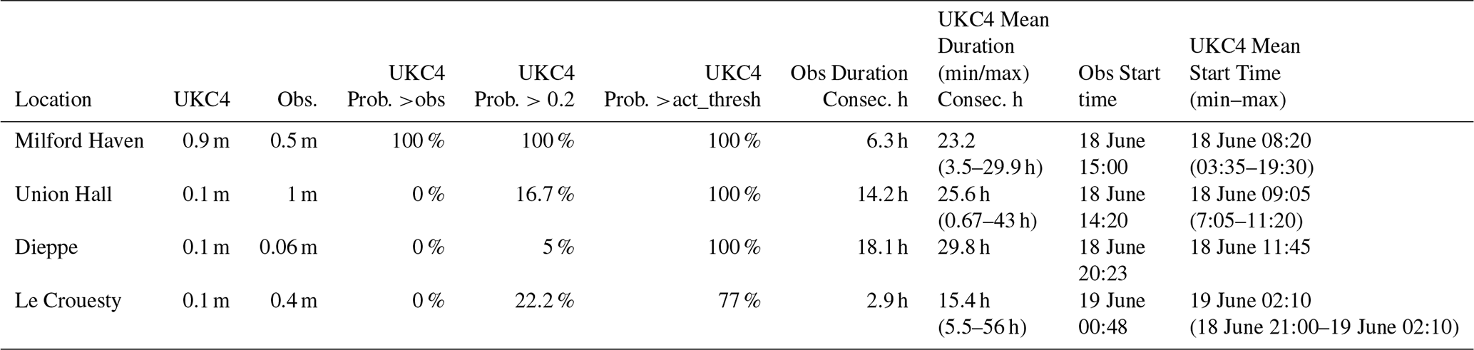
Focusing on Milford Haven, where the strongest meteotsunami signal was captured by the system, we find that the timing and duration of the event is successfully captured by the ensemble with one-day lead time (Fig. 19, top) but the intensity is often overestimated, with 89 % of the members capturing an enhanced signal compared to the observations (>0.4 m) and all members capturing the minimum threshold of meteotsunami amplitude of 0.2 m. The event starting time is 18 June 15:00 UTC in the observations, and ranges from 10:15 to 16:54 UTC with an average of 12:55 UTC in the UKC4 ensemble (Table 2). The three-day lead ensemble forecast (Fig. 19, bottom) is still very skillful, with all ensemble members showing an amplitude larger than 0.2 m, and 66.7 % members showing an amplitude of 0.4 m or more. However, the ensemble spread in start times increases to a 03:35–19:30 UTC window three days in advance and the duration is often overestimated (Table 3).

To conclude, an ensemble forecast of this event would have been skillful to represent the amplitude, duration and timing of the meteotsunami event one day in advance, although with an overestimation of its amplitude. With 3-d lead times, the forecast still provides high confidence of a meteotsunami event happening on the 18 June.

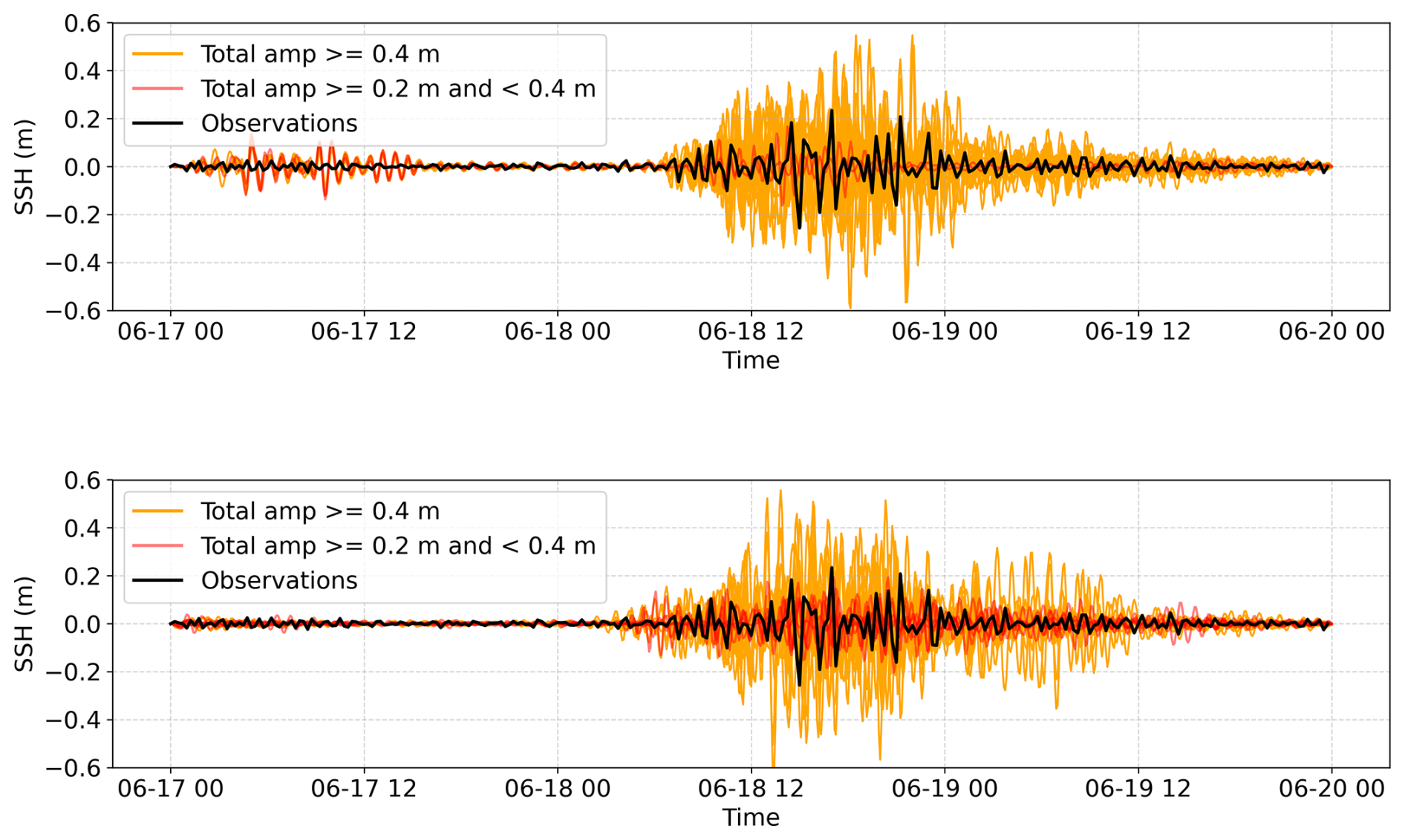
Figure 19 Ensembles forecasting for 1 d ahead the event (17 June 2022, top) and 3 d ahead of the event (15 June 2022, bottom). Orange: forecast members which reach the meteotsunami threshold of 0.2 m; Red: forecast members between meteotsunami threshold (0.2 m) and peak signal observed at Milford Haven (0.4 m).

5.2 Metrics of Ensemble Forecast

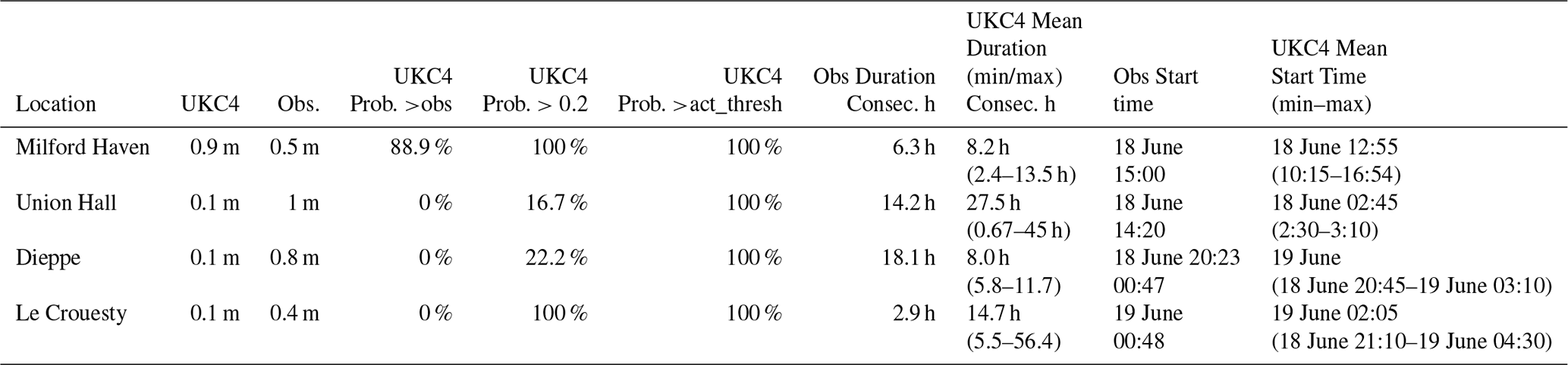
To assess forecast uncertainty, we include a set of ensemble-based statistics from the UKC4 system at each country’s location showing the strongest observed signals: Milford Haven, Union Hall, Dieppe, and Le Crouesty. Tables 2 and 3 summarise the statistics for forecasts issued 1 and 3 d in advance, respectively. Each table reports the maximum signal simulated by UKC4 alongside the corresponding observed values. We further estimate the probability that the UKC4 signal exceeds three predefined thresholds. (a) the observed signal at each location. This provides a direct measure of the model’s ability to reproduce or surpass the magnitude of the observed event. (b) the minimum meteotsunami threshold (0.2 m) (c) Given the model’s limitation to sometimes capture the full amplitude of the meteotsunami signal, but still showing a significant signal in comparison to its own baseline of variability, we define a third threshold based on a scaled increase in model variability (hereafter referred to as the activity threshold), defined as:

$$\begin{array}{}\text{(2)}& \begin{array}{rl}\mathrm{activity}\mathrm{\_}\mathrm{threshold}& ={\mathit{\sigma }}_{\mathrm{model},\mathrm{day}\mathrm{1}}\\ & \cdot \left({\displaystyle \frac{{\mathit{\sigma }}_{\mathrm{obs},\mathrm{meteotsunami}\mathrm{\_}\mathrm{duration}}}{{\mathit{\sigma }}_{\mathrm{obs},\mathrm{day}\mathrm{1}}}}\right)\end{array}\end{array}$$

where σ denotes the standard deviation of the filtered signal. “Day 1” refers to the first forecast day, during which no meteotsunami activity is present, used to calculate “baseline variability”. “Model” corresponds to each UKC4 ensemble member, and “obs” denotes observations. The observed meteotsunami duration at each location is defined as the interval between first and last time steps when the absolute value of the filtered signal is above 0.1 m (half the meteotsunami threshold).

The duration of the event for the model at a given location is then defined as interval between first and last time steps when the absolute value of the filtered signal is above the activity threshold. We add a condition that duration is only counted for members which maximum amplitude still exceed the minimum theoretical meteotsunami signal threshold of 0.2 m. These values are reported in the tables alongside the corresponding observed duration and start time.

Overall, the 1 d lead forecasts presented in Table 2 indicate that the model is able to show the possibility of a signal which would qualify as meteotsunami (>0.2 m) for all the sites, ranging from 16.7 % in Union Hall (Ireland) to 100 % in Milford Haven (UK) and Le Crouetsy (France). All the members also show considerable increase in filtered SSH variability compared to the 17 June for all sites (> activity threshold), indicating a strong likelihood of abnormal high-pass sea level variations. The model is only able to predict the observed values of meteotsunami amplitude for Milford Haven.

Regarding the start time of the event, the observed start time is within the interval predicted by the ensemble for two sites (Milford Haven and Le Crouetsy), and slightly off by 20 min for Dieppe. In Union Hall, however, the model starts the event 12 h earlier than observed. The duration of the event is more difficult to predict: the range of durations indicated by the model is large, indicating weak skills to determine the exact event duration. Nevertheless, the ensemble mean duration shows absolute errors ranging from 1.9 h (Milford Haven) to 11.8 h (Le Crouesty).

At longer lead times (Table 3), the overall skill decreases, as reflected by reduced probabilities of exceeding the minimum criteria for meteotsunami amplitude (0.2 m) and increased spread in both duration and timing estimates. Nevertheless, the model retains high probabilities of enhanced filtered SSH variability on the 18 and 19 June compared to 17 June suggesting that while amplitude prediction remains challenging, the model can still provide useful indications of potential meteotsunami occurrence on 18 and 19 June.

Table 2 UKC4 forecasting performance at 1-d lead time for selected locations. Reported values include the modelled (UKC4) and observed peak signals, along with the probability of exceeding three thresholds: 0.2 m, the activity threshold (act_thresh), and the observed peak. Event characteristics are summarised by the duration of consecutive hours above the activity threshold and the event start time. For UKC4, mean duration and start time across ensemble members are shown, with minimum and maximum values provided in parentheses. When minimum and maximum values are not reported, the timings are identical across all ensemble members.

Table 3 Same as Table 2 but for 3-d lead time.

6 Discussion

6.1 Overcoming Observation and Model Barriers to Understand and Forecast Meteotsunamis

The importance of forecasting short-period sea-level disturbances such as meteotsunamis in UK coastal waters has been increasingly recognised in recent years, as highlighted by several studies (Thompson et al., 2020; Lewis et al., 2023; Renzi et al., 2023). Despite this growing attention, our understanding of these events remains limited, largely due to the inadequacy of existing observational and forecasting infrastructure. Notably, the spatial and temporal resolution of tide gauge networks around the UK is generally insufficient for capturing meteotsunamis, as most gauges record data at 15-min intervals which is too coarse to resolve these high-frequency phenomena, as highlighted by Lewis et al. (2023). Although some signals can still be detected with 15-min intervals (as demonstrated for UK locations in this case study), the clarity and accuracy of the signal can be compromised when high-frequency disturbances occur. This is illustrated in Fig. A3, where the sampling rate of observations at Union Hall – where the largest signal of 1 m was recorded – was reduced to 15 min. The figure clearly shows that when resampled to a lower recording frequency, the first peak is entirely missed, highlighting the critical importance of high-frequency observations for accurately capturing such events. Similarly, light vessels in the Channel measure pressure at 1 h intervals, which is not frequent enough to identify sub-hourly pressure disturbances, and could not be used for model validation in this study. High-frequency pressure sensors, offshore buoys, and lightships, should be equipped with rapid sampling capabilities. These platforms could provide crucial data to enhance understanding, improve model validation, and support the development of early-warning systems for meteotsunamis.

In addition to observational limitations, conventional operational forecast systems, even with high resolution, are driven by coarse resolution models with at best 1 h forcing intervals (Tonani et al., 2019; Berthou et al., 2025). We show for the first time that km-scale regional coupled systems exchanging information at 10 min frequency, developed at the Met Office and Météo-France, offer opportunity to better understand and forecast meteotsunamis in shallow shelf regions. Although coupling is likely not useful for the feedback themselves as the sea surface height is not send back to the atmosphere, 10 min frequency forcing of a high resolution atmospheric model is too expensive to store and process to be used as forcing to an ocean model: adopting coupling for ocean forecasting becomes a more efficient solution (Berthou et al., 2025).

6.2 Success and Challenges in Representing and Forecasting Meteotsunamis

In this study, we examine the meteotsunami event previously analysed by Renzi et al. (2023), shifting the focus from tide gauge observations to the performance of high-resolution, high-frequency regional coupled systems in representing such events. Specifically, we assess the ability of two coupled systems to simulate the meteotsunami: the UKC4 system from the Met Office, which integrates the Unified Model (UM) at 1.5 km resolution, WAVEWATCH III, and NEMO at 1.5 km resolution (Berthou et al., 2026), and the AROBASE system from Météo-France, which couples the 1.3 km AROME atmospheric model with a 1.8–2.4 km NEMO ocean model (Pianezze et al., 2022). All models are operated with a 10 min coupling frequency.

The UKC4 system detects meteotsunami signals, whereas the AROBASE system exhibits substantially reduced skill, particularly in regions close to the edge of its domain, such as Ireland and Wales (Fig. 3). A key mechanism for meteotsunami generation is Proudman resonance, which occurs when the speed of the atmospheric pressure disturbance matches the phase speed of long ocean waves (Vilibić et al., 2021; Lewis et al., 2023; Renzi et al., 2023). For the resonance to be effective, the pressure anomaly must travel with a nearly constant translational speed over a sufficiently long duration and along a long-enough stretch of ocean with constant shallow depth (Wijeratne and Pattiaratchi, 2024). For this particular case, the AROBASE system has too weak and too fast pressure disturbances to maintain this critical resonance condition in most locations, resulting in weak or undetectable SSH signals. In contrast, UKC4 demonstrates a more consistent alignment between atmospheric speed and ocean phase speed, thereby maintaining conditions conducive to Proudman resonance and producing a more realistic meteotsunami response. This is further supported by the filtered OASIS mean sea-level pressure (MSLP) analysis (Figs. 9–12), which indicates that pressure perturbations are stronger over the UK and Ireland in the UKC4 system, while they are more pronounced over France in the AROBASE system. However, as both systems exhibit similarly accurate spatial representations of MSLP in their atmospheric components (Fig. 7), the discrepancy likely arises from faster-propagating gravity waves in AROME than in UM, limiting the system’s ability to generate Proudman resonance in the ocean system (Figs. 8 and 13).

Our findings further support previous research (e.g., Renzi et al., 2023; Wijeratne and Pattiaratchi, 2024; Vilibić et al., 2008): meteotsunamis require a subtle combination of many conditions, and if one is missing, they do not develop. In this case, we demonstrated that the rare co-occurrence of several meteotsunamis in 3 different countries required a slow-moving surface frontal system with a very intense density gradient, with an upper-level front triggering elevated convection sending downdrafts into a near-surface stable frontal layer, which triggered low-level organised gravity waves and surface convection, traveling at the correct speed on a long-enough stretch of constant-depth shallow ocean. This combination of events shows the complexity of meteotsunamis and highlights the prowess of representing them in a forecasting system, demonstrated in this study.

UKC4 illustrates that even a small shift in the speed of travel of the stable layer itself led to underestimation of the meteotsunami on Irish coasts and overestimation on British coasts. The less organised nature of gravity-waves in the Channel led to weaker intensities there (Fig. 4), and interestingly, their different propagation speed in UKC4 and AROBASE led to the first having a better signal on the British coast, excited with faster-moving signal, and the latter having better signal in Dieppe, a very shallow region excited by slower waves.

Finally, both systems show a weak meteotsunami signal in the Bay of Biscay (Fig. 5), although the pressure signal is quite strong in the atmospheric models, with organised convective system/gravity waves. We suspect the propagation of the system is not in the right direction for this region, highlighting another key ingredient.

Nevertheless, both systems showed a good timing of the signal in various locations, and although they often underestimated the full meteo-tsunami amplitude, they could still be useful early-warning tools. It is important to note that amplitude underestimations may also result from coastal resolution limitations, which prevent the system from capturing additional resonant effects (e.g., within harbours) or from the proximity of certain locations to the edge of the model domain. The fact that the combination of conditions is crucial for meteotsunamis to develop also calls for an ensemble approach to their forecasting.

Meteotsunamis are not currently forecast within the Northwest European Shelf region. Our analysis using ensemble forecasts from the Met Office's regional coupled model indicates that this event can be predicted with relatively high accuracy up to 24 h in advance, and with moderate accuracy up to three days in advance. This opens up the possibility of establishing early warning systems, which could significantly aid flood risk management and potentially save lives, given the documented fatalities associated with meteotsunami events (Lewis et al., 2019).

6.3 Filling the Research Gap on Meteotsunamis with Kilometer-Scale Regional Coupled Systems

A key research gap in the study of meteotsunamis lies in the detailed understanding of the atmospheric conditions that trigger these events, particularly when multiple meteotsunamis are observed over a wide area. In this case, the meteotsunami event was driven by convective activity embedded within a strongly stratified frontal system. While previous studies have attributed meteotsunami generation primarily to low-pressure frontal systems (Renzi et al., 2023), our findings suggest that such an explanation is insufficient to account for the complex and widespread sea surface disturbances observed during this event.

Through a comprehensive analysis of atmospheric conditions, we demonstrate that this event was initiated by downdraft interactions with a surface-based stable layer, which enabled the formation of gravity waves and surface-based convection. These convective structures became organised and propagated parallel to the southwest–northeast-oriented stable layer along the front. The resulting gravity waves formed coherent bands that sequentially affected the Celtic Sea, the western English Channel, and the Bay of Biscay, becoming more disorganised as they progressed into the eastern Channel. From this it can be concluded that although simpler frontal systems may trigger localised meteotsunamis (as shown in Berthou et al., 2025), more complex synoptic conditions can produce widespread and high-magnitude events, such as the 1-m meteotsunamis observed in this case.

Spatial analyses using UKC4 (Fig. 6) show that the system can reliably reproduce meteotsunami signals across the domain, allowing us, for the first time, to visualise their spatial structure and extent.

7 Conclusions

This paper presents an analysis of the meteotsunami event on 18 June 2022, which affected a broad area including the UK, Ireland, and France, and produced the highest recorded meteotsunami amplitude in Ireland (1 m). While previously examined using observations (Renzi et al., 2023), the atmospheric origin of the triggering pressure disturbances had not been fully explained. Here, we analyse the event using 2 km-scale regional coupled systems: the UKC4 system from the Met Office (Unified Model, NEMO, and WAVEWATCH III) and the AROBASE system from Météo-France (AROME and NEMO), both employing 10-min coupling to resolve meteotsunami dynamics.

Model outputs were compared against tide gauge data from the affected regions, with sea level and pressure data filtered using a high-pass Butterworth filter (cutoff 1.5 min) to isolate short-period signals. Pressure disturbances are mainly analysed using model outputs, as observational data at most locations lack sufficient temporal resolution for meaningful comparison; Brest and Le Havre are the only exceptions. UKC4 captured the event particularly well in the Celtic Sea, simulating a 0.9 m amplitude, close to the observed 1 m, though with a spatial offset. It showed reduced performance in the English Channel and Bay of Biscay but still produced signals near the 0.2 m meteotsunami threshold, demonstrating potential for early warning. In contrast, AROBASE was less successful in capturing the event, particularly in the Celtic Sea, where it produced little to no signal, though it showed modest improvement in the English Channel and Bay of Biscay. These underestimations, especially in AROBASE, are attributed to the system's limited ability to simulate Proudman resonance for this particular case, where atmospheric and oceanic wave speeds align, amplifying the sea level signal. Notably, UKC4 enabled, for the first time, a clear spatial representation of the meteotsunami signal. Additionally, some limitations may arise from the systems' resolutions, particularly when further amplification occurs along the coastline due to features such as harbours and other fine-scale structures that the system cannot adequately resolve. Indeed, with 1.5 km (UKC4) and 1.8–2.4 km (AROBASE) and a minimum depth of 10 m, the NEMO-based ocean models of this study cannot by design represent finer-scale seiching than twice their grid-scale – hence missing most of the harbour resonance, estuary resonance or coastal amplification by energy conservation. One way to address this would be to increase the ocean model resolution; however, this usually comes with a decrease in domain size to balance costs, which could then miss the shelf-wide amplification of meteotsunamis. Using an unstructured grid with variable resolution in the ocean would enable this compromise, but NEMO does not offer this feature and the cost of supporting a different system than NEMO is prohibitive for both the Met Office and Météo France. Since most of the meteotsunami signal can already be effectively captured from UKC4, and its ensemble forecasts supports the development of an early warning system, we believe that increasing the resolution is not sufficiently justified in this context.

Atmospheric analysis addressed a key gap in meteotsunami research by identifying the triggering mechanism: convective activity within a strongly stratified frontal system, combined with downdraft interactions in a surface-based stable layer, generated gravity waves and surface-based convection. These organised along a southwest–northeast-oriented front, initiating meteotsunamis over a wide area.

Ensemble forecasts using UKC4 showed strong potential for predicting such events up to 24 h in advance, and with moderate skill up to 3 d, highlighting its value for early warning applications – particularly for activating flood defences and reducing risk to life.

This study also underscores the importance of high-frequency sea level and pressure observations for detecting, understanding, and forecasting meteotsunamis. Such data are critical for model validation and early warning system development.

In conclusion, kilometer-scale regional coupled systems, when combined with appropriate observations, offer a promising path toward improved understanding and forecasting of meteotsunamis. Future research should focus on additional case studies to refine the evaluation of both modeling systems, to assess false alarms/hit rate ratio of the systems and enhance ensemble-based operational forecasting. Deploying high-resolution, high-frequency coupled system in climate mode will also bring a better understanding of the likelihood of these events: their frequency is currently four events per year, with one significant event every five years (Lewis et al., 2023). However, convective systems are predicted to become more intense, and possibly slower-moving (Chan et al., 2020; Kahraman et al., 2021), which could potentially combine into greater probability of meteotsunamis.

Future work could include test cases with the standalone NEMO configurations used in this study with idealised atmospheric pressure forcing (Proudman/Greenspan/edge-wave test, Proudman, 1929; Greenspan, 1956), to reveal whether the issues with the AROBASE system come from the ocean or the atmospheric model configuration. In addition, assessing the operational performance of meteotsunami prediction through a systematic analysis of false alarm and hit rate ratios across multiple cases will be an important step toward improving forecast reliability.

Appendix A

Full range of the meteotsunami signal (filtered timeseries) for Union Hall and Milford Haven, where the peaks occur can be seen in Fig. A1:

When resampling all datasets (UKC4 and AROBASE outputs) to match the 15 min sampling frequency at Milford Haven (Fig. A2), a slight attenuation of the signal is observed in UKC4. Nevertheless, the overestimation by UKC4 remains pronounced. This suggests that while resampling can influence the representation of the meteotsunami signal, the primary source of discrepancy appears to be the propagation speed of the stable layer as simulated by UKC4. Comparable results were obtained at other locations (not shown).

The importance of high-frequency observational data is further illustrated for Union Hall in Fig. A3. At Union Hall – the site of the highest recorded signal – it is evident that resampling at 5 min observation (without adjusting the model output) can lead to a substantial reduction in the observed amplitude. This underscores the value of high-frequency observations for accurately capturing meteotsunami amplitude.

Comparisons to the MSLP stations used in Renzi et al. (2023) are shown here for reference. One needs to note that only two locations are in the AROBASE domain while recording frequency is 1 h.

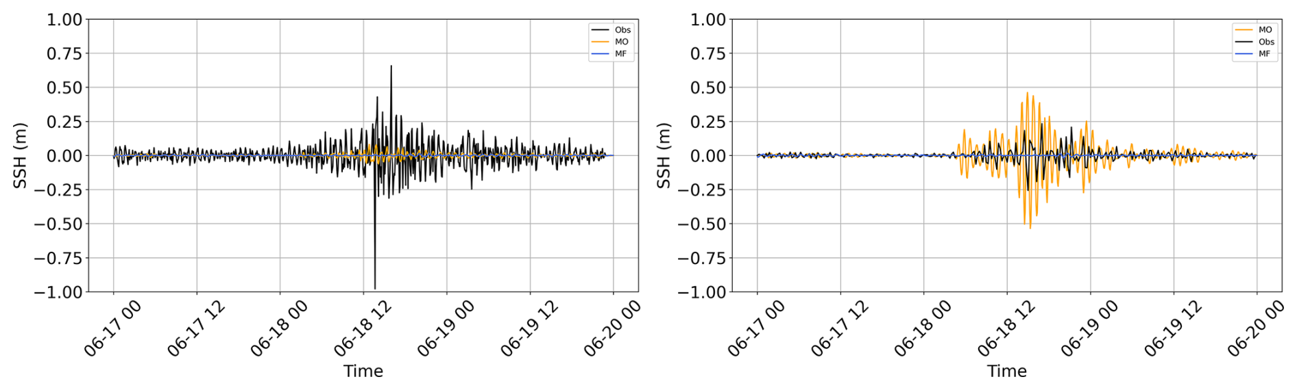
Figure A1 Full range of filtered sea surface height for Union Hall (left) and Milford Haven (right), where peak of meteotsunami signal occurred. Observations are in black, with 15 min frequency for the UK stations and 5 min for Irish stations. Model outputs are in orange (UKC4) and blue (AROBASE) and have 5 min frequency. The locations of the observations are shown in Fig. 2.

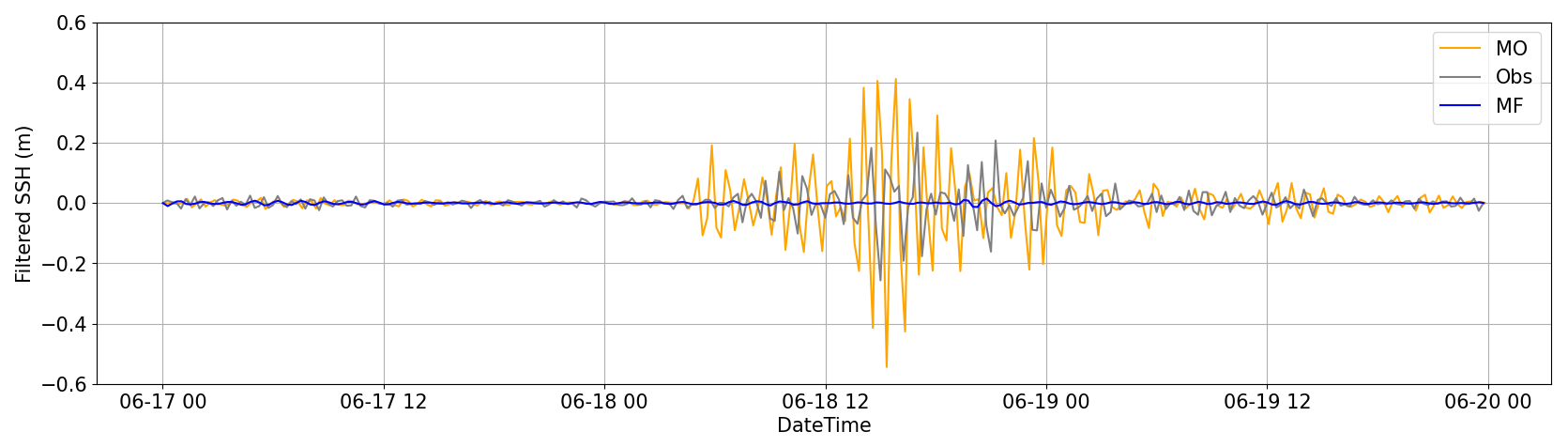
Figure A2 Filtered SSH time series at Milford Haven after resampling, comparing UKC4 (orange) and AROBASE (blue) against observations (grey).

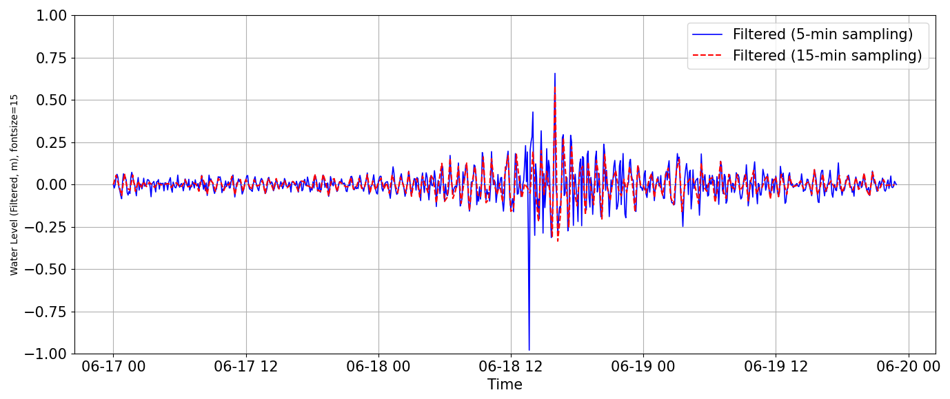
Figure A3 SSH Filtered Timeseries for Union Hall observations when resampling from 5 min (blue) to 15 min (red).

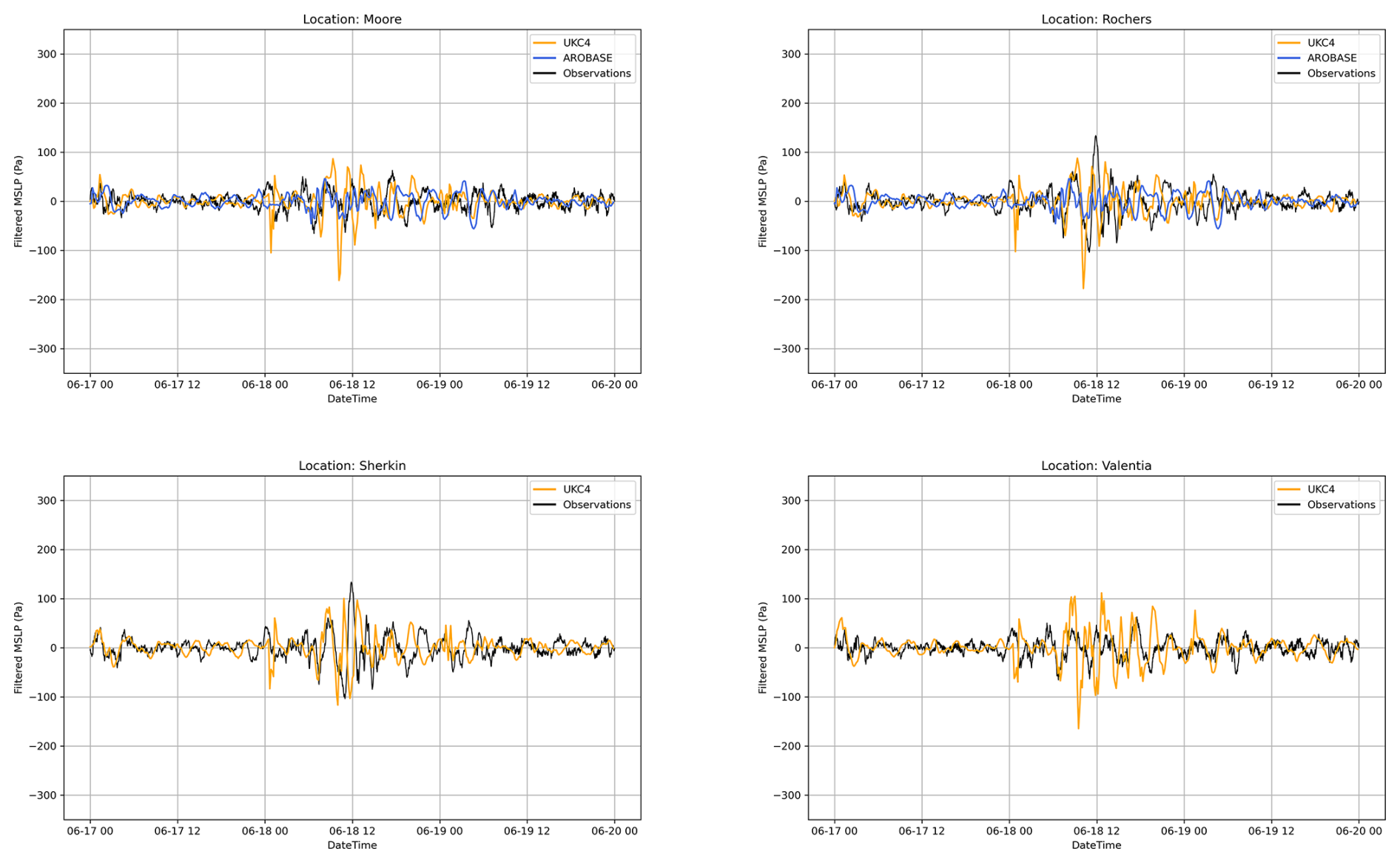
Figure A4 Filtered MSLP time series from UKC4 (orange) and AROBASE (blue) at the four Irish locations used in Renzi et al. (2023). The same 6-h cutoff and Butterworth high-pass filter are applied here.