Meteorological Drought Trend Analysis and Forecasting Using a Hybrid SG-CEEMDAN-ARIMA-LSTM Model Based on SPI from Rain Gauge Data

Meteorological drought presents considerable challenges to water supplies, agriculture, and socio-economic stability, especially in areas heavily reliant on precipitation. The Standardized Precipitation Index (SPI) is esteemed for its efficacy in drought monitoring, owing to its straightforwardness and applicability across many time scales. This study examines meteorological drought dynamics in the uMkhanyakude district using the Standardized Precipitation Index (SPI) at 6-, 9-, and 12-month timescales. Trend analysis was conducted using Mann–Kendall (MK), Modified Mann–Kendall (MMK), and Innovative Trend Analysis (ITA) methods. The study also proposes a hybrid model that integrates the Savitzky–Golay (SG) filter, Complete Ensemble Empirical Mode Decomposition with Adaptive Noise (CEEMDAN), Autoregressive Integrated Moving Average (ARIMA), and Long Short-Term Memory (LSTM) networks, referred to as SG-CEEMDAN-ARIMA-LSTM, for forecasting of the SPI time series. Analysis of SPI trends and variability revealed statistically significant declining trends at five monitoring stations, characterized by negative Z-scores and p-values, showing a marked downward trajectory across several SPI scales. On the other hand, the forecasting results demonstrate that the SG-CEEMDAN-ARIMA-LSTM methodology outperformed benchmark models across all temporal scales, achieving high prediction accuracy with R² values of 0.9839 (SPI-6), 0.9892 (SPI-9), and 0.9990 (SPI-12). These findings highlight the effectiveness of decomposition techniques (SG, CEEMDAN) in enhancing model performance and confirm the suitability of the hybrid model for both short-term and long-term drought forecasting. This study merges robust trend analysis with advanced hybrid forecasting techniques, providing a reliable framework for early warning systems and sustainable water resource management in drought-prone regions.

1 Introduction

Drought is a complex and recurring natural hazard with significant economic, social, and environmental implications globally (Bagmar and Khudri, 2021; Kalisa et al., 2021; Song and Park, 2021). In contrast to other natural disasters, droughts manifest gradually, often persisting for extended periods, and their effects permeate various sectors, including agriculture, water resources, and socio-economic systems (Wilhite and Glantz, 1985; Cunha et al., 2019). This study specifically focuses on meteorological drought, characterized as a sustained period of below-average precipitation (Taylan, 2024). Meteorological drought often serves as the initial phase that subsequently evolves into agricultural, hydrological, and socioeconomic drought (Malik et al., 2021; Latifoğlu and Özger, 2023). As it is solely influenced by precipitation variability, meteorological drought can be effectively quantified using precipitation-based indices.

Several indices have been established to quantify drought conditions, including the Standardized Precipitation Index (SPI) and the Standardized Precipitation Evapotranspiration Index (SPEI). While the SPEI integrates both precipitation and temperature data, its requirement for extensive datasets and complex computations may restrict its applicability in regions with limited data availability (Xu et al., 2020). Conversely, the SPI depends exclusively on precipitation, rendering it widely used for analysing meteorological drought, especially in semi-arid regions. Its versatility across multiple timescales facilitates the robust identification of both short- and long-term drought patterns. Accordingly, given the data constraints in the uMkhanyakude district of South Africa, this study adopts the SPI as the primary drought index, while recognizing that its exclusive reliance on precipitation constitutes a methodological limitation. Since SPI is precipitation-driven, analysing rainfall trends is a necessary first step before applying SPI under climate change conditions. Without first establishing rainfall trends, one risks misinterpreting SPI signals as short-term anomalies when they may actually reflect long-term climate-driven shifts.

In this context, the escalating concerns regarding climate change and its influence on local climates have underscored the necessity of analyzing drought trends. Thus, trend analysis of rainfall and SPI together provides a comprehensive picture of rainfall trends, revealing the climatic forcing, while SPI trends quantify the standardized drought intensity and persistence, which is crucial for understanding drought risk in the context of climate change. Systematic evaluations of drought occurrences not only contribute to the development of evidence-based water resource management strategies but also enhance the calibration of early warning systems and inform climate adaptation policies at both regional and national levels. Furthermore, temporal analyses enable researchers to assess the effectiveness of mitigation measures and anticipate emerging risks, thereby bolstering resilience in vulnerable sectors such as agriculture and public water supply. In the absence of structured trend analyses, drought management remains predominantly reactive, constraining the transition towards proactive and sustainable adaptation strategies. Building on trend analysis, drought forecasting is essential for deepening the understanding of drought dynamics. Effective forecasting provides early warnings that are critical for mitigating impacts and strengthening drought management strategies (Balti et al., 2020; Zhang et al., 2022, 2024; Tan et al., 2023).

Accurate forecasting of the SPI is crucial in regions such as uMkhanyakude, which is prone to recurrent and severe drought events. Enhanced prediction capabilities support agricultural resilience, water resource planning, and the establishment of early warning systems (Xu et al., 2020). Traditional statistical models, such as ARIMA or SARIMA, alongside contemporary machine learning methods, have been extensively employed for forecasting drought indices, including the SPI. However, each approach has inherent limitations. For example, Gudko et al. (2025) utilized SARIMA to analyze precipitation dynamics in Russia, demonstrating efficacy in short-term predictions while exhibiting constrained accuracy for long-term forecasts. Similarly, Hussain et al. (2025) integrated ARIMA with machine learning models to enhance SPI and SPEI predictions, achieving accuracies exceeding 92 %. This highlights the advantages of combining statistical and machine learning techniques. Nonetheless, these methodologies often encounter challenges associated with nonlinear and complex rainfall patterns, particularly over short time scales. To mitigate the limitations of standalone models, hybrid approaches have gained prevalence, capitalizing on the complementary strengths of diverse techniques. Alquraish et al. (2021) compared hybrid models such as HMM-GA, ARIMA-GA, and ARIMA-GA-ANN against, such as HMM-GA, ARIMA-GA, and ARIMA-GA-ANN, with conventional HMM and ARIMA models for SPI prediction in the Arabian Peninsula, revealing that hybrid models consistently outperformed their standalone counterparts. Likewise, Xu et al. (2022) and Ding et al. (2022) demonstrated that the combination of CEEMD with ARIMA or LSTM significantly improves SPI forecasts across multiple time scales in China, suggesting that decomposition-based hybrid methods effectively capture intricate temporal patterns.

Recent studies have significantly advanced hybrid methodologies through the implementation of sophisticated preprocessing and optimization techniques. Latifoğlu and Özger (2023) utilized phase transfer entropy (pTE) in conjunction with Tunable Q Factor Wavelet Transform (TQWT), optimized via Grey Wolf Optimization (GWO), followed by artificial neural networks (ANN), support vector regression (SVR), machine learning (ML), and Gaussian process regression (GPR), resulting in superior predictive performance. Sibiya et al. (2024) introduced the CEEMDAN-ARIMA-LSTM model for SPI predictions in Cape Town, demonstrating that the combination of CEEMDAN decomposition with both linear and nonlinear models can significantly improve forecast accuracy. Wei et al. (2025) adopted the Informer model and developed the VMD-JAYA-Informer hybrid, which integrates Variational Mode Decomposition (VMD) with an optimization algorithm, thereby enhancing short-term Standardized Precipitation Index (SPI) and Standardized Precipitation-Evapotranspiration Index (SPEI) forecasts.

Despite the successes achieved by hybrid models, several challenges persist. Decomposition techniques such as Empirical Mode Decomposition (EMD), Ensemble Empirical Mode Decomposition (EEMD), Complete Ensemble Empirical Mode Decomposition with Adaptive Noise (CEEMDAN), and Variational Mode Decomposition (VMD) are computationally demanding, particularly when applied to large datasets or in real-time contexts (Sibiya et al., 2024). CEEMDAN, specifically, can yield misleading intrinsic mode functions (IMFs) when utilized on excessively noisy or unstable time series, which undermines the efficiency and reliability of subsequent predictions. Furthermore, existing research has not investigated the synergistic application of advanced smoothing filters in conjunction with decomposition techniques to mitigate noise prior to hybrid modeling.

To address these limitations, this study proposes an innovative hybrid model that integrates the Savitzky-Golay (SG) filter with CEEMDAN for preprocessing, followed by the Autoregressive Integrated Moving Average (ARIMA) and Long Short-Term Memory (LSTM) models for drought prediction. The SG filter is effective in smoothing high-frequency noise, thereby enhancing the decomposition process and alleviating the computational burden. The integration of the Savitzky-Golay smoothing filter with CEEMDAN substantially improves forecasting accuracy by enhancing the quality and interpretability of the input time series prior to modeling. This combination enables CEEMDAN to produce IMFs that are cleaner, more distinct, and less prone to spurious fluctuations, thus offering a more reliable foundation for subsequent predictive modeling. Cleaner IMFs facilitate the training of both linear (ARIMA) and nonlinear (LSTM) models, resulting in more accurate and robust forecasts. This approach capitalizes on the complementary strengths of both statistical and machine learning models, addressing noise-related issues inherent in raw data.

Although hybrid models have demonstrated superior performance in drought forecasting, no prior study has examined:

1. The combined use of smoothing techniques (SG filter) with CEEMDAN to enhance the quality of decomposition.

2. The implementation of an integrated SG-CEEMDAN-ARIMA-LSTM framework for trend-based Standardized Precipitation Index (SPI) predictions (SPI-6, SPI-9, SPI-12).

3. Forecasting efforts that explicitly incorporate both trend analysis and predictive modeling for semi-arid regions characterized by limited meteorological data.

As a result, the proposed SG-CEEMDAN-ARIMA-LSTM model addresses these gaps by enhancing decomposition efficiency, reducing computational costs, and improving prediction accuracy across multiple SPI timescales. This methodology offers valuable insights for water resource management, infrastructure planning, early warning systems, and the advancement of hybrid drought prediction models.

2 Material Methods

This study utilizes various time series forecasting models to analyse the intricate dynamics of meteorological drought as indicated by the Standardized Precipitation Index (SPI). The foundational statistical model examined is the Autoregressive Integrated Moving Average (ARIMA), which is adept at addressing linear relationships in time series data. The Long Short-Term Memory (LSTM) neural network is employed to tackle nonlinear patterns, supplemented by a hybrid ARIMA-LSTM framework that amalgamates the advantages of both models. Additional improvements are investigated by incorporating a Savitzky-Golay (SG) digital smoothing filter, which is often used to remove noise from time series or spectral data, into the ARIMA-LSTM model, and by utilizing the Complete Ensemble Empirical Mode Decomposition with Adaptive Noise (CEEMDAN) before ARIMA-LSTM to more effectively manage nonstationary signals. The work introduces a unique hybrid model, SG-CEEMDAN-ARIMA-LSTM, which integrates decomposition and hybrid modeling techniques to enhance the accuracy and robustness of drought forecasts.

Therefore, the subsequent Materials and Methods section will provide a detailed account of the study area, the data employed, and the preprocessing steps undertaken, including the trend extraction methods applied prior to forecasting. This will be followed by an in-depth description of each modeling approach, outlining their theoretical foundations, implementation procedures, and parameterization strategies. Such a structured presentation ensures transparency in model development and establishes a comprehensive methodological framework for the proposed forecasting system.

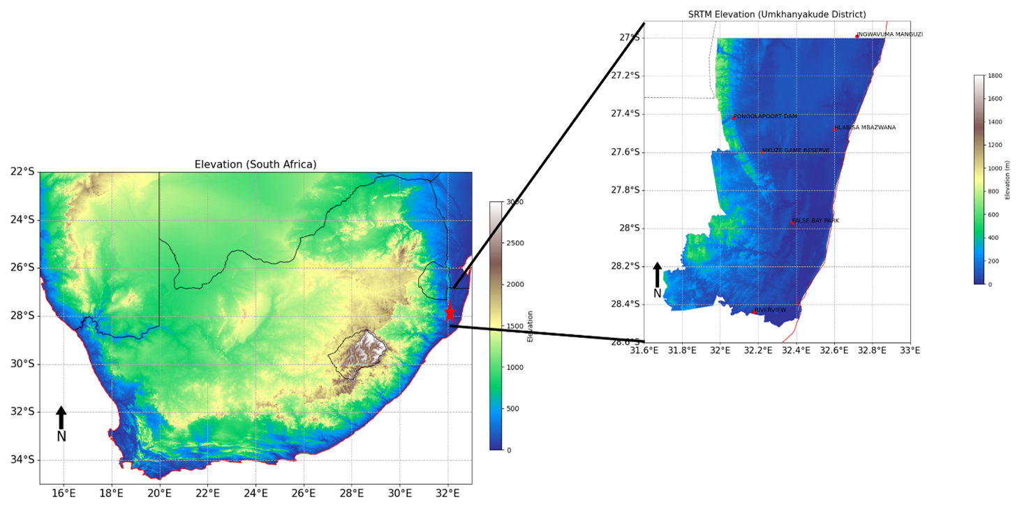
Figure 1 Overview of the uMkhanyakude District, South Africa. Rain gauge stations are marked red.

2.1 Study Area and Data

This study employed monthly mean precipitation records from 1980 to 2023, obtained from the South African Weather Service (SAWS) for the uMkhanyakude District in South Africa. The uMkhanyakude District Municipality is located in the far northern region of the KwaZulu-Natal (KZN) province (coordinates: 32.014489° S, 27.622242° E). The municipality covers a total area of 13 855 km², making it the second largest in the province, exceeded only by the Zululand Municipality. The uMkhanyakude District was formed immediately after the local government elections in December 2000, as part of the municipal demarcation process, encompassing some of the most destitute and underdeveloped areas of KwaZulu-Natal. The uMkhanyakude District consists of four local municipalities: uMhlabuyalingana, Jozini, Big Five Hlabisa, and Mtubatuba. The municipality is geographically surrounded by Mozambique to the north, the Indian Ocean to the east, the uThungulu River to the south, Zululand to the west, and the Kingdom of Swaziland to the northwest. Figure 1 illustrates the spatial distribution of the stations.

Figure 2 The Box-Jenkins Steps Approach.

2.2 Modified Mann-Kendall

The modified Mann-Kendall methodology is derived from the nonparametric Mann-Kendall method (Mann, 1945; Kendall, 1975), which is widely used to detect trends in hydro-meteorological time series (Caloiero et al., 2011; Bard et al., 2015; Wang et al., 2017; Mirabbasi et al., 2020). The modified Mann–Kendall (MMK) test was employed for serially correlated data exhibiting a substantial lag-1 autocorrelation coefficient, utilising the variance correction method proposed by Yue et al. (2002). Hamed and Rao (1998) created this methodology to eradicate all substantial autocorrelation in the time series. Under the assumption that the data are independent and identically distributed, the S statistic of the Mann-Kendall test is computed as follows (Sharifi et al., 2024):

$$\begin{array}{}\text{(1)}& S=\sum _{i=\mathrm{1}}^{n-\mathrm{1}}\sum _{j=i+\mathrm{1}}^n\mathrm{Sign}\left(x_j-x_i\right)\end{array}$$

where n denotes the sample size; x_i and x_j denote sequential ith and jth data points, respectively, and sign(.) is the sign function which can be computed as

$$\begin{array}{}\text{(2)}& \mathrm{Sign}\left(x_j-x_i\right)=\left\{\begin{array}{l}\mathrm{1},\mathrm{if}{x}_j-x_i>\mathrm{0}\\ \mathrm{0},\mathrm{if}{x}_j-x_i=\mathrm{0}\\ -\mathrm{1},\mathrm{if}{x}_j-x_i<\mathrm{0}\end{array}\right.\end{array}$$

with the mean and variance of the S statistics in the equation are as follows (Helsel and Hirsch, 1993; Ma et al., 2014; Ashraf et al., 2023)

$$\begin{array}{}\text{(3)}& {\displaystyle }E\left(S\right)=\mathrm{0}\text{(4)}& {\displaystyle }\mathrm{Var}\left(S\right)={\displaystyle \frac{n\left(n-\mathrm{1}\right)\left(\mathrm{2}n+\mathrm{5}\right)-{\sum }_{i=\mathrm{1}}^p{t}_i(t_i-\mathrm{1})\left(\mathrm{2}{t}_i+\mathrm{5}\right)}{\mathrm{18}}}\end{array}$$

where p is the number of tied groups and t_i denotes the number of data points in the tth group. The second term represents an adjustment for tied group or censored data. The standardized Z statistic is calculated as

$$\begin{array}{}\text{(5)}& Z_{\mathrm{MK}}=\left\{\begin{array}{l}\frac{S-\mathrm{1}}{\sqrt{\mathrm{Var}\left(S\right)}},S>\mathrm{0}\\ \mathrm{0},S=\mathrm{0}\\ \frac{S+\mathrm{1}}{\sqrt{\mathrm{Var}\left(S\right)}},S<\mathrm{0}\end{array}\right.\end{array}$$

The test statistic Z is used to measure the significance of the trends. In the modified Mann-Kendall approach, a modified variance of S is computed as follows (Hamed and Rao, 1998)

$$\begin{array}{}\text{(6)}& \mathrm{Var}\left(S^{\ast }\right)=\mathrm{Var}\left(S\right){\displaystyle \frac{n}{n^{\ast }}}\end{array}$$

where n^∗ is the effective sample size. The $\frac{n}{n^{\ast }}$ ratio can be calculated as follows (Hamed and Rao, 1998)

$$\begin{array}{}\text{(7)}& \begin{array}{rl}{\displaystyle \frac{n}{n^{\ast }}}& =\mathrm{1}+{\displaystyle \frac{\mathrm{2}}{n(n-\mathrm{1})(n-\mathrm{2})}}\sum _{i=\mathrm{1}}^n\left(n-i\right)\\ & \left(n-i-\mathrm{1}\right)\left(n-i-\mathrm{2}\right)r_i\end{array}\end{array}$$

where r_i denotes the lag-i significant autocorrelation coefficient of rank i in a time series. Then the standardized statistic of the S statistic, denoted as Z, can be derived as

$$\begin{array}{}\text{(8)}& Z_{\mathrm{MMK}}=\left\{\begin{array}{l}\frac{S-\mathrm{1}}{\sqrt{\mathrm{Var}\left(S^{\ast }\right)}},S>\mathrm{0}\\ \mathrm{0},S=\mathrm{0}\\ \frac{S+\mathrm{1}}{\sqrt{\mathrm{Var}\left(S^{\ast }\right)}},S<\mathrm{0}\end{array}\right.\end{array}$$

If the calculated Z values (Z_MK and Z_MMK) exceed the critical values of $-Z_{\mathrm{1}-\mathit{\alpha }/\mathrm{2}}$ or fall below $Z_{\mathrm{1}-\mathit{\alpha }/\mathrm{2}}$, there is no discernible trend in the time series at the significance level of α. If the Z value is positive and exceeds $Z_{\mathrm{1}-\mathit{\alpha }/\mathrm{2}}$, the trend is upward; conversely, if the Z value is negative and falls below $-Z_{\mathrm{1}-\mathit{\alpha }/\mathrm{2}}$, the trend is downward.

Figure 3 Structure diagram of LSTM model.

2.3 Innovative Trend Analysis

The Innovative Trend Analysis (ITA) method, initially introduced by Şen (2012), has been widely employed for detecting patterns in precipitation time series. Since its debut, the ITA technique has experienced substantial improvements in both mathematical and graphical aspects, as evidenced by Şen (2017) and Alashan (2018). The ITA method does not depend on assumptions of serial autocorrelation, normalcy, or record length, making it appropriate for both graphical and statistical trend analysis (Zena et al., 2022). Initially, the time series is bifurcated into two equal segments and organised in ascending order. The initial segment of the time series ($x_i:i=\mathrm{1},\mathrm{2},\mathrm{\dots },n/\mathrm{2}$) is positioned along the horizontal x-axis, while the subsequent segment ($x_j:j=n/\mathrm{2}+\mathrm{1},n/\mathrm{2}+\mathrm{2},\mathrm{\dots },n$) is situated along the vertical y-axis in the Cartesian coordinate system (Ashraf et al., 2023). The ITA approach visually represents trend analysis, specifically indicating monotonic growing, declining, and trendless circumstances (Öztopal and Şen, 2017; Likinaw et al., 2023). A monotonically growing or declining trend can be identified when the majority of points are situated above or below the 45° (1:1 line), respectively. A trendless condition arises when the data points are clustered along the 45° line (Şen, 2012). We employ the magnitude of the slope parameter to convey information about monotonicity. The slope parameter of the ITA technique is a stochastic property dependent on the sample means of the first half (n₁) and the second half (n₂) of the time-series mean data values. According to Şen (2017), the straight-line trend slope (S_ITA) can be estimated using the following expression:

$$\begin{array}{}\text{(9)}& S_{\mathrm{ITA}}={\displaystyle \frac{\mathrm{2}x\left(x_j-x_i\right)}{n}}\end{array}$$

where n represents the total number of observations, x_i and x_j are the arithmetic means of the first and second halves of the sub-series, respectively. Given that x_i and x_j are stochastic variables, the expected value of the slope can be determined by analysing the expectancies of both the first and second halves of the time series (Alashan, 2020; Harka et al., 2021):

$$\begin{array}{}\text{(10)}& E\left(S_{\mathrm{ITA}}\right)={\displaystyle \frac{\mathrm{2}}{n}}\left[E\left(x_j\right)-E\left(x_i\right)\right]\end{array}$$

For the no trend condition, E(x_j)=E(x_i), the E(S_ITA)=0 and standard deviation (SD) of the two half time-series $\left({\mathit{\sigma }}_{x_j}={\mathit{\sigma }}_{x_i}=\mathit{\sigma }/\sqrt{n}\right)$, σ is the SD is of the parent series. If E(x_j)≠E(x_i), the differences between E(x_j) and E(x_i) gives the variance

$$\begin{array}{}\text{(11)}& {\mathit{\sigma }}_{S_{\mathrm{ITA}}}^{\mathrm{2}}={\displaystyle \frac{\mathrm{8}}{n^{\mathrm{2}}}}\left[E\left(x_j\right)-E\left(x_j{x}_i\right)\right]\end{array}$$

and the SD of the slope

$$\begin{array}{}\text{(12)}& {\mathit{\sigma }}_{S_{\mathrm{ITA}}}={\displaystyle \frac{\mathrm{2}\sqrt{\mathrm{2}}}{n\sqrt{n}}}\mathit{\sigma }\sqrt{\mathrm{1}-{\mathit{\rho }}_{x_j{x}_i}}\end{array}$$

In the stochastic processes, the term ${\mathit{\rho }}_{x_j{x}_i}$ is the correlation coefficient between the two mean values, and can be estimated as

$$\begin{array}{}\text{(13)}& {\mathit{\rho }}_{x_j{x}_i}={\displaystyle \frac{E\left(x_j{x}_i\right)-E\left(x_j\right)E\left(x_i\right)}{{\mathit{\sigma }}_{x_j}{\mathit{\sigma }}_{x_i}}}\end{array}$$

In the end, the upper and lower confidence limit (CL) of the trend slope was calculated (Şen, 2017):

$$\begin{array}{}\text{(14)}& {\mathrm{CL}}_{(\mathrm{1}-\mathit{\alpha })}=\mathrm{0}\pm \left(Z_{\mathrm{1}-\mathit{\alpha }/\mathrm{2}}\right){\mathit{\sigma }}_{S_{\mathrm{ITA}}}\end{array}$$

$Z_{\mathrm{1}-\mathit{\alpha }/\mathrm{2}}$ denotes the crucial slope for standardised time-series at ±1.96 for a 95 % significance level or ±1.645 for a 90 % significance level (Alashan, 2020). If the ITA slope value is beyond the lower and upper confidence limits, the null hypothesis of no significant trend should be rejected at the α significance level (Şen, 2017). In a two-tailed scenario, the null hypothesis (H₀) posits the absence of a trend in time-series data, while the alternative hypothesis (H₁) asserts the presence of a trend in time-series data at a significance level of α. If the slope, $\pm S_{\mathrm{ITA}}>\pm {\mathrm{CL}}_{(\mathrm{1}-\mathit{\alpha })}$, then (H₀) is discarded in favour of (H₁). The positive and negative values of S_ITA signify an upward and downward trend in the time-series data, respectively (Şen, 2017).

2.4 The SPI Calculation

For the purpose of analysing the severity of drought, which is caused by a lack of water supply as a result of reduced precipitation in response to rising demand, the SPI was created by McKee et al. (1993) and is based on probability (Zuo et al., 2021). Based on the cumulative likelihood of a specific amount of precipitation, the SPI indicator is calculated by fitting the precipitation throughout the same period with a certain distribution function. At its largest point, the SPI index represents the quantile of a normal distribution. Each time axis has an estimated drought index for 6, 9, and 12 months. This is based on the gamma probability density function, which accounts for the periodic distribution of precipitation for the corresponding data point. The expression of the density function for this distribution is as follows.

$$\begin{array}{}\text{(15)}& g\left(x\right)={\displaystyle \frac{\mathrm{1}}{{\mathit{\beta }}^{\mathit{\alpha }}\mathrm{\Gamma }\left(\mathit{\alpha }\right)}}{x}^{\mathit{\alpha }-\mathrm{1}}{e}^{-\frac{x}{\mathit{\beta }}}\end{array}$$

where α is the shape parameter, β is the scale parameter and x is the precipitation amount, and $\mathrm{\Gamma }\left(\mathit{\alpha }\right)={\int }_{\mathrm{0}}^{\mathrm{\infty }}{y}^{\mathit{\alpha }-\mathrm{1}}{e}^{-y}\mathrm{d}y$ is gamma function. The maximum likelihood estimates of the parameters α and β are:

$$\begin{array}{}\text{(16)}& {\displaystyle }\mathit{\alpha }={\displaystyle \frac{\mathrm{1}}{\mathrm{4}A}}\left(\mathrm{1}+\sqrt{\mathrm{1}+{\displaystyle \frac{\mathrm{4}A}{\mathrm{3}}}}\right)\text{(17)}& {\displaystyle }\mathit{\beta }={\displaystyle \frac{\stackrel{\mathrm{‾}}{x}}{n}}\end{array}$$

where $A=\ln \left(\stackrel{\mathrm{‾}}{x}\right)-\frac{\sum \ln \left(x\right)}{n}$, $\stackrel{\mathrm{‾}}{x}$ is the precipitation average and n is the sample size. The following equation applies the acquired parameters to the cumulative probability distribution:

$$\begin{array}{}\text{(18)}& G\left(x\right)=\underset{\mathrm{0}}{\overset{x}{\int }}g\left(x\right)\mathrm{d}x={\displaystyle \frac{\mathrm{1}}{{\mathit{\beta }}^{\mathit{\alpha }}\mathrm{\Gamma }\left(\mathit{\alpha }\right)}}\underset{\mathrm{0}}{\overset{x}{\int }}{x}^{\mathit{\alpha }-\mathrm{1}}{e}^{-\frac{x}{\mathit{\beta }}}\mathrm{d}x\end{array}$$

G(x) represents the likelihood that the precipitation will be equal to or less than x. The distribution function for precipitation needs to be adjusted because the real precipitation samples can contain a value of 0. Based on this, we can calculate the cumulative probability as:

$$\begin{array}{}\text{(19)}& H\left(x\right)=q+\left(\mathrm{1}-q\right)G\left(x\right)\end{array}$$

where q denotes the probability when precipitation equals zero. The probability of no rainfall, q, can be articulated as $q=m/r$, where m represents the number of days without rainfall and r denotes the number of days with rainfall (Song and Park, 2021). Consequently, H(x) is converted to the conventional random variable Z of the standard normal distribution, characterised by a mean of 0 and a variance of 1, resulting in:

$$\begin{array}{}\text{(20)}& {\displaystyle }\mathrm{SPI}=Z=\left\{\begin{array}{l}-\left(k-\frac{c_{\mathrm{0}}+c_{\mathrm{1}}k+c_{\mathrm{2}}{k}^{\mathrm{2}}}{\mathrm{1}+d_{\mathrm{1}}k+d_{\mathrm{2}}{k}^{\mathrm{2}}+d_{\mathrm{3}}{k}^{\mathrm{3}}}\right),\mathrm{0}<H\left(x\right)\le \mathrm{0.5}\\ +\left(k-\frac{c_{\mathrm{0}}+c_{\mathrm{1}}k+c_{\mathrm{2}}{k}^{\mathrm{2}}}{\mathrm{1}+d_{\mathrm{1}}k+d_{\mathrm{2}}{k}^{\mathrm{2}}+d_{\mathrm{3}}{k}^{\mathrm{3}}}\right),\mathrm{0}<H\left(x\right)\le \mathrm{1.0}\end{array}\right.\text{(21)}& {\displaystyle }k=\left\{\begin{array}{l}\sqrt{\ln \left({\left(\frac{\mathrm{1}}{H\left(x\right)}\right)}^{\mathrm{2}}\right)},\mathrm{0}<H\left(x\right)<\mathrm{0.5}\\ \sqrt{\ln \left({\left(\frac{\mathrm{1}}{\mathrm{1}-H\left(x\right)}\right)}^{\mathrm{2}}\right)},\mathrm{0}<H\left(x\right),<\mathrm{1.0}\end{array}\right.\end{array}$$

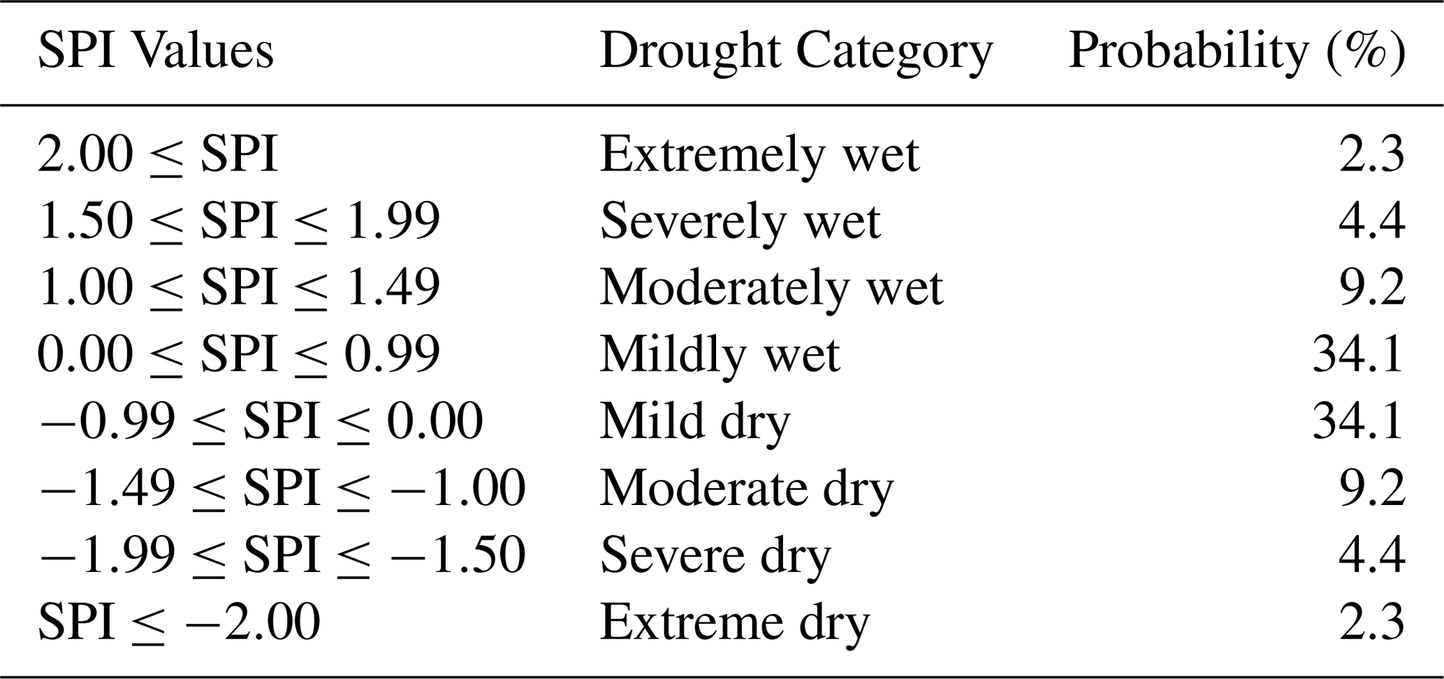
where $c_{\mathrm{0}}=\mathrm{2},\mathrm{515517}$, c₁=0.802853, $c_{\mathrm{2}}=\mathrm{0},\mathrm{010328}$, $d_{\mathrm{1}}=\mathrm{1},\mathrm{432788}$, $d_{\mathrm{2}}=\mathrm{0},\mathrm{189269}$, $d_{\mathrm{3}}=\mathrm{0},\mathrm{001308}$ are constants. Furthermore, the SPI indicator is a standardised normalised index, establishing a correlational relationship with likelihood. Table 1 presents the probability associated with each category of drought.

Figure 4 Predictive flowchart of the ARIMA-LSTM hybrid model.

Figure 5 Procedure of proposed SG-CEEMDAN-ARIMA-LSTM hybrid model.

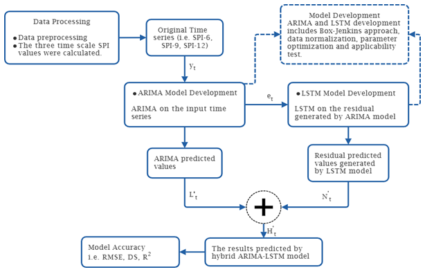
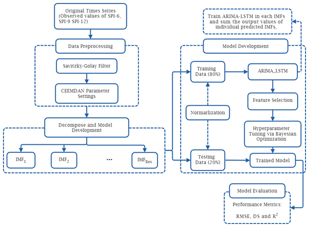
Table 1 Drought classification using SPI values and corresponding event probability (Lloyd-Hughes and Saunders, 2002).

2.5 The Savitzky-Golay Filter

The Savitzky-Golay (SG) smoothing technique is a widely used method for noise filtration. Savitzky and Golay (1964) introduced the SG filter as an effective technique for signal smoothing. The SG technique attenuates noise utilising two parameters: polynomial order and window size. By flexibly adjusting these two parameters, the SG filter can achieve exceptional performance in various pre-processing circumstances. The essence of this procedure involves fitting a low-degree polynomial to the samples within a sliding window using the least squares method, resulting in a new smoothed value for the central point derived by convolution. The SG filter is a specific variant of a low-pass filter that substitutes each value in the time series with a new value derived from a polynomial fit to 2m+1 surrounding points, including the point to be smoothed, where m is equal to or larger than the polynomial's order. The polynomial is articulated as follows:

$$\begin{array}{}\text{(22)}& p\left(n\right)=\sum _{k=\mathrm{0}}^N{a}_k{n}^k\end{array}$$

where N is the power of the polynomial and $N\le \mathrm{2}M+\mathrm{1}$. The following equation is used to determine the error between the estimated and original values; in order to find the desired polynomial result, this error must be minimised.

$$\begin{array}{}\text{(23)}& {\mathit{ϵ}}_N=\sum _{n=-M}^M{\left(p\left(n\right)-x\left[n\right]\right)}^{\mathrm{2}}\end{array}$$

The following form of discrete convolution can be used to express the filter's output:

$$\begin{array}{}\text{(24)}& y\left[n\right]=\sum _{m=-M}^{M}h\left[m\right]x[n-m]=\sum _{m=n-M}^{n+M}h\left[n-m\right]x\left[m\right]\end{array}$$

This work employs the SG filter for two primary reasons: firstly, it enhances system performance by preserving the width and height of waveform peaks in noisy SPI, and secondly, it modifies the SPI while maintaining its fundamental qualities.

2.6 The Complete Ensemble Empirical Mode Decomposition with Adaptive Noise

The model's ability to fit functions and converge will be constrained by the complexity and volatility of the original time sequence, which in turn limits the model's predictive power. To overcome this challenge, the complete ensemble empirical mode decomposition (CEEMDAN) technique is employed to preprocess the original nonstationary and nonlinear time series. Both empirical mode decomposition (EMD) and ensemble empirical mode decomposition (EEMD), have been enhanced by the CEEMDAN. The computational efficiency is improved, and the reconstructed sequences of both the EMD and EEMD algorithms are free of modal confusion and noise residuals (Zhang et al., 2023). A residual term and a sequence of intrinsic mode functions (IMFs) are the building blocks of a complicated time series signal that the CEEMDAN breaks down.

Step 1: Incorporate a constrained quantity of adaptive white noise into the original sequence $x\left(t\right){\mathit{\delta }}_{\mathrm{0}}{\mathit{\omega }}^i\left(t\right)(t=\mathrm{1},\mathrm{2},\mathrm{3},\mathrm{\dots },N)$

$$\begin{array}{}\text{(25)}& x^i\left(t\right)=x\left(t\right)+{\mathit{\delta }}_{\mathrm{0}}{\mathit{\omega }}^i\left(t\right)\end{array}$$

where N denotes the number of trials, δ₀ signifies a coefficient of intensity, and ωⁱ(t) indicates the ith realisation of a stochastic Gaussian process.

Step 2: The residual r₁(t) and the first modal component IMF₁ are obtained by decomposing each Eq. (1) using EMD.

$$\begin{array}{}\text{(26)}& {\displaystyle }\stackrel{\mathrm{‾}}{{\mathrm{IMF}}_{\mathrm{1}}\left(t\right)}={\displaystyle \frac{\mathrm{1}}{N}}\sum _{i=\mathrm{1}}^N{\mathrm{EMD}}_{\mathrm{1}}\left(x^i\left(t\right)\right)\text{(27)}& {\displaystyle }{r}_{\mathrm{1}}\left(t\right)=x\left(t\right)-\stackrel{\mathrm{‾}}{{\mathrm{IMF}}_{\mathrm{1}}\left(t\right)}\end{array}$$

In this context, EMD₁(.) denotes the initial IMF component produced by the EMD algorithm, while r₁(t) signifies the residual associated with the first stage.

Step 3: Add white noise δ₁EMD₁(ωⁱ(t)) to the residual r₁(t) and further decomposed by EMD to obtain the second modal component IMF₂ and residual r₂(t).

$$\begin{array}{}\text{(28)}& {\displaystyle }\stackrel{\mathrm{‾}}{{\mathrm{IMF}}_{\mathrm{2}}\left(t\right)}={\displaystyle \frac{\mathrm{1}}{N}}\sum _{i=\mathrm{1}}^N{\mathrm{EMD}}_{\mathrm{1}}\left(r_{\mathrm{1}}\left(t\right)+{\mathit{\delta }}_{\mathrm{1}}{\mathrm{EMD}}_{\mathrm{1}}\left({\mathit{\omega }}^i\left(t\right)\right)\right)\text{(29)}& {\displaystyle }{r}_{\mathrm{2}}\left(t\right)=r_{\mathrm{1}}\left(t\right)-\stackrel{\mathrm{‾}}{{\mathrm{IMF}}_{\mathrm{2}}\left(t\right)}\end{array}$$

For the $j=\mathrm{3},\mathrm{4},\mathrm{\dots },N$, the jth IMF component and the jth residual can be computed as:

$$\begin{array}{}\text{(30)}& {\displaystyle }\stackrel{\mathrm{‾}}{{\mathrm{IMF}}_j\left(t\right)}={\displaystyle \frac{\mathrm{1}}{N}}\sum _{i=\mathrm{1}}^N{\mathrm{EMD}}_{\mathrm{1}}\left(r_{j-\mathrm{1}}\left(t\right)+{\mathit{\delta }}_{j-\mathrm{1}}{\mathrm{EMD}}_{j-\mathrm{1}}\left({\mathit{\omega }}^i\left(t\right)\right)\right)\text{(31)}& {\displaystyle }{r}_j\left(t\right)=r_{j-\mathrm{1}}\left(t\right)-\stackrel{\mathrm{‾}}{{\mathrm{IMF}}_j\left(t\right)}\end{array}$$

where ${\mathrm{EMD}}_{j-\mathrm{1}}(.)$ denotes the (j−1)th intrinsic mode function component derived from the empirical mode decomposition technique, and r_j(t) represents the residual following the jth decomposition.

Step 3: Continue executing step 3 until the residual r_j(t) meets a predetermined termination criterion.

The time series x(t) can ultimately be articulated as

$$\begin{array}{}\text{(32)}& x\left(t\right)=\sum _{i=\mathrm{1}}^N\stackrel{\mathrm{‾}}{{\mathrm{IMF}}_N\left(t\right)}+r_N\left(t\right)\end{array}$$

2.7 The Autoregressive Integrated Moving Average Model

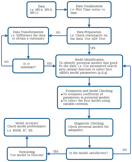
The Autoregressive Integrated Moving Average (ARIMA) model, pioneered by Box and Jenkins in the 1970s, serves as a robust and effective forecasting approach for time series analysis (Box et al., 2015). The ARIMA model, often known as the Box-Jenkins approach, is depicted through the concepts presented by Sibiya et al. (2024) in Fig. 2. The ARIMA models predict future values of the time series as a linear combination of historical and residual data. This model comprises three components: the order of seasonal differentiation, autoregressive order, and moving average order (Montgomery et al., 2015). The backward shift operator B is employed to eliminate nonstationarity. A time series, y_t, is called homogeneous nonstationary if it first order difference, ${\mathit{\omega }}_y=\left(\mathrm{1}-B\right)y_t=y_t-y_{t-\mathrm{1}}$ or the dth difference ${\mathit{\omega }}_t={\left(\mathrm{1}-B\right)}^d{y}_t$ is also stationary time series. Furthermore, y_t is referred to as an ARIMA model with orders pd and q, noted ARIMA(pdq). Hence, an ARIMA(pdq) is often expressed as

$$\begin{array}{}\text{(33)}& {\displaystyle }\mathit{\varphi }\left(B\right){\left(\mathrm{1}-B\right)}^d{y}_t=c+\mathit{\theta }\left(B\right){\mathit{\epsilon }}_t\text{(34)}& {\displaystyle }\mathit{\varphi }\left(B\right)=\mathrm{1}-\sum _{i=\mathrm{1}}^p{\mathit{\varphi }}_i{B}^i\mathrm{and}\mathit{\theta }\left(B\right)=\mathrm{1}-\sum _{i=\mathrm{1}}^q{\mathit{\theta }}_i{B}^i\end{array}$$

The backward shift operators for AR(p) and MA(q) are defined as $\mathit{\varphi }\left(B\right)y_t=c+{\mathit{\epsilon }}_t$ and $y_t=\mathit{\mu }+\mathit{\theta }\left(B\right){\mathit{\epsilon }}_t$ with $c=\mathit{\mu }-\mathit{\varphi }\mathit{\mu }$, where μ and ε_t are the mean and white noise, respectively and the ε_t is independent and normal distributed with mean and variance of ${\mathit{\sigma }}_{\mathit{\epsilon }}^{\mathrm{2}}$.

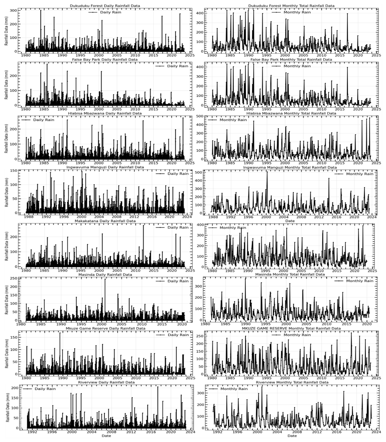
Figure 6 Time series plots of daily and monthly total rainfall data for uMkhanyakude district from early 1980's to 2023. The (left) plot shows the daily rainfall data in millimeters (mm), illustrating the high variability and intermittent nature of daily rainfall events over the years. The (right) plot presents the monthly total rainfall data (mm), which smooths out the daily variability and reveals clearer patterns of rainfall distribution over time.

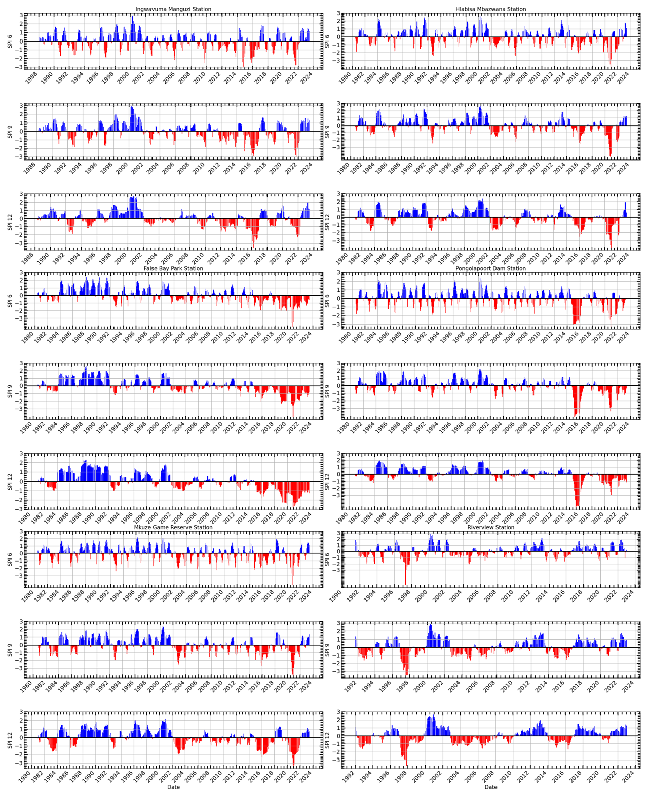
Figure 7 Standardized Precipitation Index (SPI) time series plots for uMkhanyakude district over 6-month (SPI-6), 9-month (SPI-9), and 12-month (SPI-12) periods from early 1980's to 2023. Positive SPI values (blue bars) indicate wetter-than-normal conditions, while negative SPI values (red bars) indicate drier-than-normal conditions.

2.8 The Long Short-Term Memory

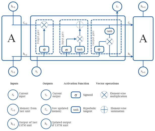
Long short-term memory (LSTM) algorithms represent a category of recurrent neural network (RNN) designs that are proficient in handling sequential input and identifying temporal relationships (Hochreiter and Schmidhuber, 1997). LSTM networks incorporate specific memory cells and gates for the efficient management and regulation of information flow over various time steps. Consequently, they can effectively represent the data input while maintaining essential dependencies and patterns. The LSTM methodology addresses the problem of vanishing gradients encountered by RNN algorithms. This occurs when the gradient diminishes to a level insufficient for effectively updating the weights throughout prolonged sequences. The LSTM facilitates the flow of gradients across time by employing memory cells and gates. The model's foundational design primarily consists of three control gates: input, forget, and output. The activation function is represented by σ, whereas the cell states at time t−1 and t are designated as C_t−1 and C_t respectively. At time t and time t−1, the cell possesses two concealed states, h_t and h_t−1. Figure 3 illustrates the building of the LSTM unit, and the mathematical Eqs. (35) to (40) for the LSTM method are provided below. Initially, by employing the model's forget gate, we may determine the current hidden state h_t−1 and the degree to which the input x_t has been preserved. The formula is

$$\begin{array}{}\text{(35)}& f_t=\mathit{\sigma }\left(W_f{x}_t+U_f{h}_{t-\mathrm{1}}+b_f\right)\end{array}$$

Secondly, the input gate allows us to ascertain the volume of content from the input variable that can be retained in the cell state C_t

$$\begin{array}{}\text{(36)}& {\displaystyle }{i}_t=\mathit{\sigma }\left(W_i{x}_t+U_i{h}_{t-\mathrm{1}}+b_i\right)\text{(37)}& {\displaystyle }{\stackrel{\mathrm{̃}}{C}}_t={\mathit{\sigma }}_c\left(W_c{x}_t+U_i{h}_{t-\mathrm{1}}+b_i\right)\text{(38)}& {\displaystyle }{C}_t=f_t\odot C_{t-\mathrm{1}}+i_i\odot {\stackrel{\mathrm{̃}}{C}}_t\end{array}$$

The output gate of the LSTM produces outputs, and the hidden state of each cell is represented by the formula:

$$\begin{array}{}\text{(39)}& {\displaystyle }{o}_t=\mathit{\sigma }\left(W_o{x}_t+U_o{h}_{t-\mathrm{1}}+b_o\right)\text{(40)}& {\displaystyle }{h}_t=O_t\odot {\mathit{\sigma }}_h\left(C_t\right)\end{array}$$

In the aforementioned formulas, W_f, W_i, and W_o represent the weight matrices associated with the various control gates. The terms b_f, b_i, and b_o correspond to the bias terms for each respective control gate. The notation ${\stackrel{\mathrm{̃}}{C}}_t$ signifies the complete input activation vector, while the operator ⊙ (Hadamard product) indicates the element-wise multiplication of the elements between two vectors. The σ activation function quantifies the amount of information that is transmitted through the various control gates.

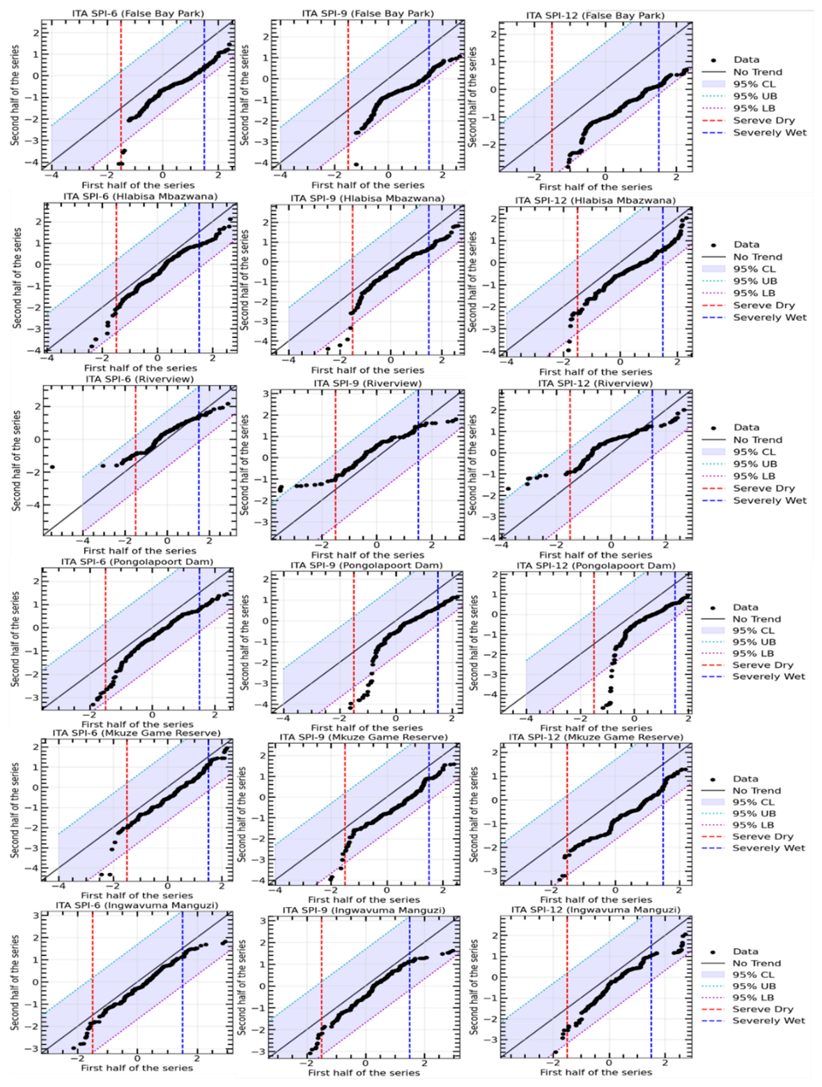
Figure 8 Results of Innovative trend analysis applied to different time scales values (SPI-6 (left), SPI-9 (middle), SPI-12 (right)). The blue shaded area represents the 95 % confidence level area. The red and blue vertical lines represent the severe drought and severely wet, respectively.

2.9 The ARIMA-LSTM hybrid Model

Achieving accurate estimates of SPI index values through a forecasting model is essential for informed decision-making. Zhang (2003) offers a hybrid model wherein the ARIMA model extracts and predicts linear components, while the residuals, representing nonlinear data subcomponents, are then modelled by the LSTM approach. This study employs a hybrid model that integrates ARIMA and LSTM to predict both linear and nonlinear behaviours with optimal accuracy.

$$\begin{array}{}\text{(41)}& H_t=L_t+{\mathrm{\aleph }}_t\end{array}$$

where L_t and ℵ_t denote the linear and nonlinear components, respectively, for the hybrid technique which are computed using the initial time series (y_t). Consider the original dataset at time t and the forecast results obtained from applying the ARIMA model as ${\widehat{L}}_t$ the prediction results. Thus, $E_t=y_t-{\widehat{L}}_t$ is the definition of the residual E_t that is derived by removing ${\widehat{L}}_t$ from y_t. Subsequently we compute the value ${\widehat{\mathrm{\aleph }}}_t$ by feeding the series of residuals into the LSTM model, which predicts the nonlinear component of the values. This equation may be written as

$$\begin{array}{}\text{(42)}& {\widehat{\mathrm{\aleph }}}_t=f_{\mathrm{LSTM}}\left(E_{t-\mathrm{1}},E_{t-\mathrm{2}},\mathrm{\dots },E_{t-n}\right)+{\mathit{ϵ}}_t,\end{array}$$

where ${\widehat{\mathrm{\aleph }}}_t$ is a nonlinear expression associated with the LSTM model and ϵ_t is the random error. The combined forecasts from the two steps were then used to determine the value for the ARIMA-LSTM hybrid model. As illustrated in Fig. 4, the equation ${\widehat{H}}_t={\widehat{L}}_t+{\widehat{\mathrm{\aleph }}}_t$ predicts the linearity and nonlinearity values, respectively, using ARIMA and LSTM models.

Table 2 Statistical summary of trend analysis for SPI-6, SPI-9, and SPI-12 using Mann-Kendall (MK) and Modified Mann-Kendall (MMK) tests.

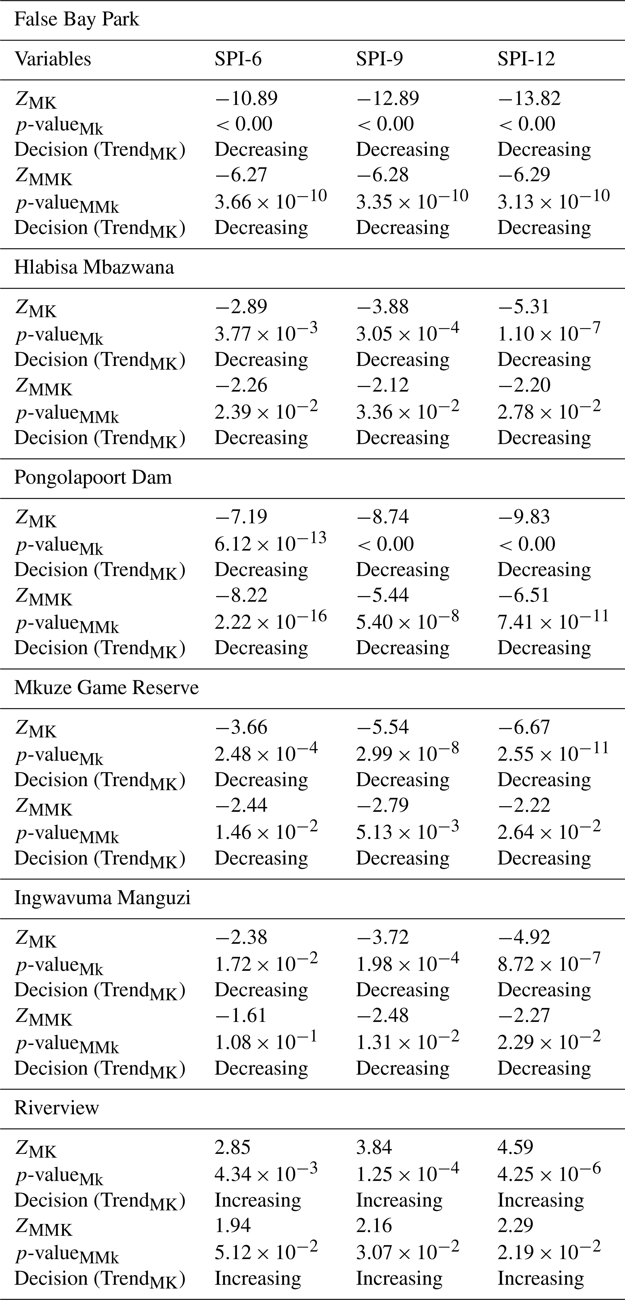
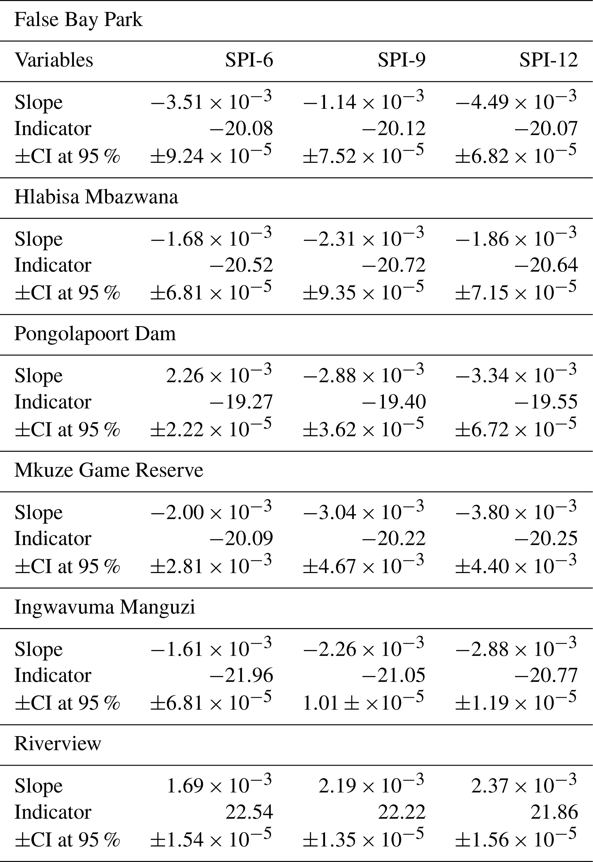
Table 3 The results of the trend analysis for SPI-6, SPI-9, and SPI-12 obtained through a two-tailed test at a significance level of 5 % using ITA technique.

2.10 The development of the proposed SG-CEEMDAN-ARIMA-LSTM hybrid model

Due to the great uncertainty of the drought data and the existence of complexity, nonlinearity, and nonstationary trends, the single prediction model is greatly limited; however, the hybrid method has better prediction accuracy. The SG-CEEMDAN-ARIMA-LSTM algorithm that combines different techniques for improved accuracy in predicting drought based on the standardised precipitation index is proposed this study. This hybrid model is designed as a sequential framework where each step refines the data for subsequent modelling. The SG-CEEMDAN pre-processing stage enhances the data by smoothing and decomposing it into the meaningful components. The benefits of integrating the Savitzky–Golay smoothing filter with CEEMDAN significantly contribute to the enhancement of forecasting accuracy by improving the quality and interpretability of the input time series prior to modeling. The Savitzky–Golay filter acts as a noise suppression mechanism that preserves essential features of the time series, while eliminating high-frequency noise. This step ensures that the input to the CEEMDAN decomposition process is already denoised, leading to more stable and physically meaningful decomposed components. The CEEMDAN generates IMFs that are cleaner, more distinct, and less affected by spurious fluctuations. This results in better mode separation, reduces signal leakage across IMFs, and enhances the stationarity and regularity of each component. This hybrid preprocessing pipeline can enhances model generalization, reduces overfitting, and ultimately leads to more reliable and accurate forecasts. The components fed to the ARIMA-LSTM model that involves two-step process: the ARIMA for initial prediction utilising the Box-Jekins methodology and the LSTM model for refining and enhancing predictions. The hybrid model combines the ARIMA and the LSTM predictions to form the final hybrid forecasts. Figure 5 illustrates the proposed hybrid model algorithm. The process of SPI prediction based on ARIMA-LSTM combined with SG and CEEMDAN as is shown in Fig. 5. The process of the data smoothing, decomposition and prediction include four main steps.

Figure 9 SPI signals smoothed by Savitzky-Golay (SG).

Step 1: Data Preprocessing Phase: To enhance the quality of the data and prepare it for decomposition, the original SPI time series undergo a data preprocessing phase:

• Savitzky–Golay Filter: This filter is applied to smooth the SPI data and preserves the essential shape and trends of the original time series while minimizing high-frequency noise. This step ensures that important signal patterns are retained during further processing. The smoothed signal becomes the input signal for decomposition technique.

• CEEMDAN Parameter Settings: CEEMDAN is used to break the smoothed signal into several IMFs and a residual component. Before decomposition, the necessary parameters for CEEMDAN are configured. These parameters control the number of realizations, noise amplitude, and stopping criteria for decomposition.

Step 2: Model Development Phase: Each IMF, including the residual, is independently modelled using a hybrid ARIMA–LSTM approach. This process involves several steps:

• a.

  Data Partitioning

  • The data for each IMF is split into: Training set (80 %) and Testing set (20 %). This split ensures that model learning and evaluation are based on separate subsets to avoid overfitting.

• b.

  Normalization

  • Prior to model training, the data is normalized using Min-Max normalization to ensure that input features fall within a similar scale, which improves training stability and convergence speed.

• c.

  Modelling Each IMF with ARIMA–LSTM

  • The two models are integrated so that both linear (ARIMA) and nonlinear (LSTM) dependencies within each IMF are effectively captured. The modelling process follows the algorithm shown in Fig. 4.

• d.

  Feature Selection and Hyperparameter Tuning

  • The performance of ARIMA and LSTM models heavily depends on the feature selection and hyperparameters. The auto_arima( ) function and Bayesian Optimization were used to automate and optimize the search for best-performing hyperparameters for the ARIMA-LSTM model by evaluating model performance over a probabilistic space.

• e.

  Model Training

  • Each IMF is trained individually using the selected features and optimized hyperparameters, resulting in a trained model for each component.

Step 3: Forecast Reconstruction Phase

• After training, each IMF is forecasted individually. The final forecasted SPI value is obtained by summing the predictions of all individual IMFs, including the residual component:

  $$\mathrm{S}\widehat{\mathrm{P}}\mathrm{I}\left(t\right)=\sum _{i=\mathrm{1}}^{n}I\widehat{M}{F}_i\left(t\right)+{\mathrm{Res}}_t$$

  This additive reconstruction ensures that the original structure and dynamics of the SPI series are preserved in the forecast, improving overall accuracy.

Step 4: Model Evaluation Phase

The reconstructed SPI prediction is then evaluated using multiple performance metrics: RMSE, DS, and coefficient of determination. The Taylor diagram is also utilised to evaluate the model performance. These metrics help quantify the predictive accuracy and reliability of the hybrid framework.

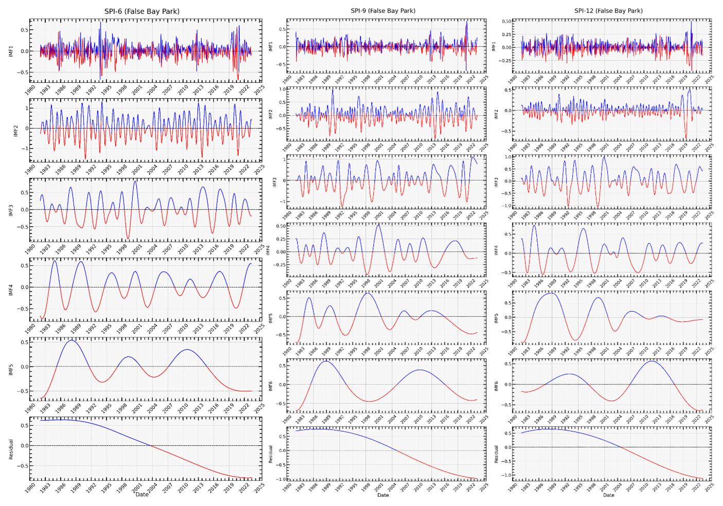
Figure 10 Decomposition of Smoothed SPI-6, SPI-9 and SPI-12 Index Using CEEMDAN: Each IMF represents different frequency components of the SPI index, from high-frequency oscillations (IMF1) to low-frequency trends (IMF5), showing the variability in precipitation patterns over the years from 1980 to 2023.

2.11 Performance Evaluation

To establish the predictive superiority of the SG-CEEMDAN-ARIMA-LSTM model, a comparison was conducted against other models, including ARIMA, LSTM, ARIMA-LSTM, SG-ARIMA-LSTM, and CEEMDAN-ARIMA-LSTM models. The performance of the proposed hybrid-based model is evaluated using three indicators namely, root mean square error (RMSE), coefficient of determination (R²) and directional symmetry (DS). The high value of R² and DS reflects the better performance of the forecasting model while the lower the value of RMSE illustrates better forecasting performance.

$$\begin{array}{}\text{(43)}& {\displaystyle }\mathrm{RMSE}=\sqrt{{\displaystyle \frac{\mathrm{1}}{n}}\sum _{i=\mathrm{1}}^n{\left(y_i-{\widehat{y}}_{\mathrm{avg}}\right)}^{\mathrm{2}}}\text{(44)}& {\displaystyle }{R}^{\mathrm{2}}={\displaystyle \frac{{\left[\sum _{i=\mathrm{1}}^n\left(y_i-y_{\mathrm{avg}}\right)\left({\widehat{y}}_i-{\widehat{y}}_{\mathrm{avg}}\right)\right]}^{\mathrm{2}}}{\sum _{i=\mathrm{1}}^n{\left(y_i-y_{\mathrm{avg}}\right)}^{\mathrm{2}}\sum _{i=\mathrm{1}}^n{\left({\widehat{y}}_i-{\widehat{y}}_{\mathrm{avg}}\right)}^{\mathrm{2}}}}\text{(45)}& {\displaystyle }\mathrm{DS}={\displaystyle \frac{\mathrm{100}}{n-\mathrm{1}}}\sum _{i=\mathrm{2}}^n{d}_i\end{array}$$

where

$$\begin{array}{}\text{(46)}& d_i=\left\{\begin{array}{l}\mathrm{1},\left(y_i-y_{i-\mathrm{1}}\right)\left({\widehat{y}}_i-{\widehat{y}}_{i-\mathrm{1}}\right)>\mathrm{0}\\ \mathrm{0},\mathrm{otherwise}\end{array}\right.\end{array}$$

n is number of data points, y_i and ${\widehat{y}}_i$ observed and forecasted, respectively. y_avg and ${\widehat{y}}_{\mathrm{avg}}$ an average of the actual and forecasted values, respectively. Furthermore, this study conducts a qualitative evaluation of the prediction model's performance using a Taylor diagram (Taylor, 2001). The Taylor diagram offers a statistical evaluation of the degree of agreement between the models in terms of their SD, RMSE, and R², while providing a concise summary of the correspondence between predicted and observed values. The differences in DS, RMSE, and R² values among the prediction models are depicted as individual points on a two-dimensional plot within the Taylor diagram. This diagram, though it follows a common structure, proves especially valuable when evaluating intricate models.

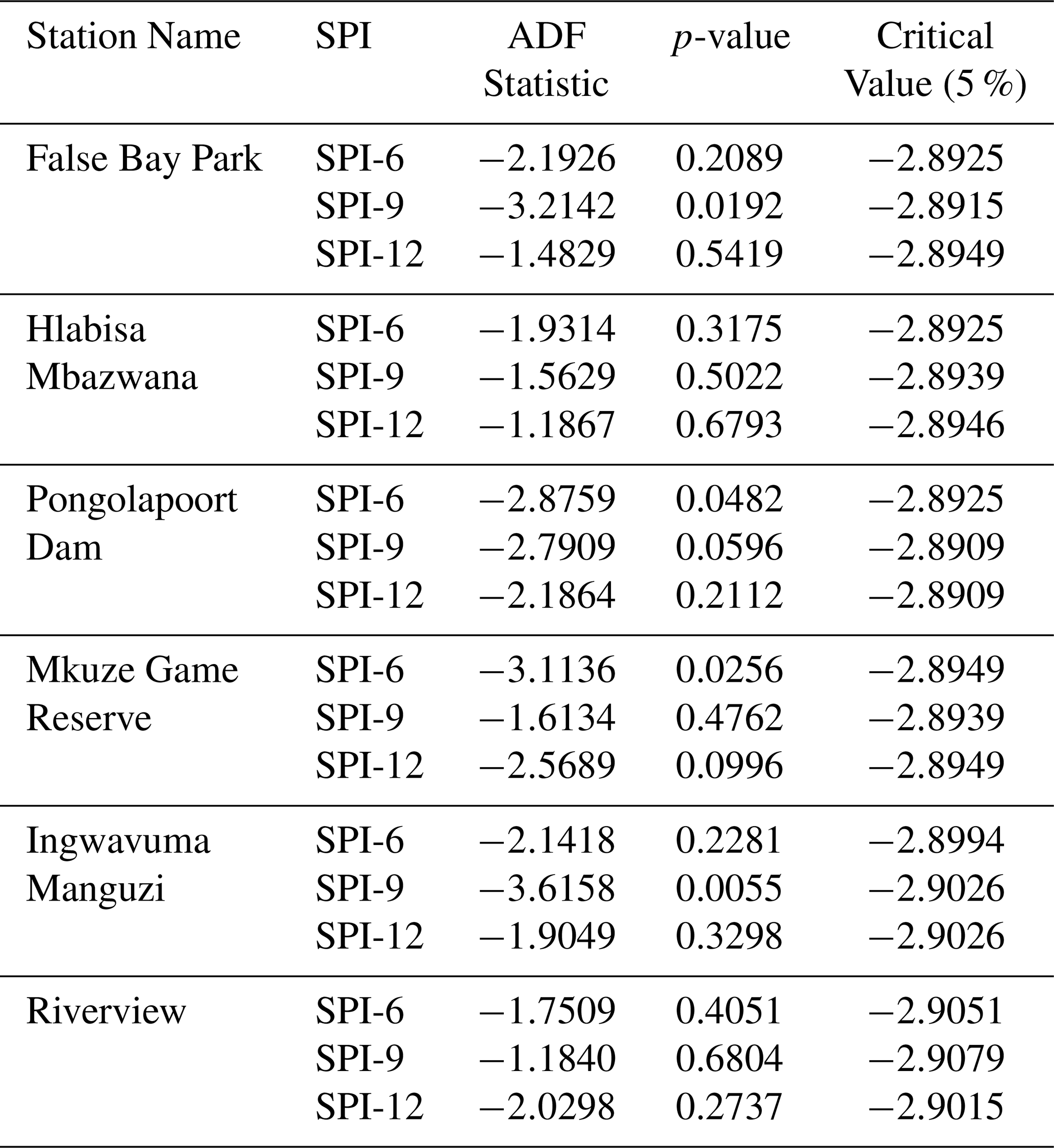
Table 4 ADF Test Results for SPI Values (SPI-6, SPI-9, SPI-12) at Different Stations.

3 Results and Discussion

3.1 Rainfall Data Series

Figure 6 illustrates the daily and monthly cumulative precipitation data recorded at the uMkhanyakude district meteorological stations in KwaZulu-Natal province, South Africa, from the early 1980s to 2023. The data comprising 20 % was employed for prediction, whereas the data representing 80 % was applied for training. The SPI was computed utilising rainfall data from meteorological stations in the uMkhanyakude district, which provide sufficiently extensive records and a consistent structure (Hırca et al., 2022).

3.2 SPI Time Series and Trend Analysis

This study SPI values for the 6-, 9-, and 12-month intervals were computed using the monthly mean time series shown in Fig. 6. Figure 7 illustrates the time series of the SPI calculated for the 6-month (SPI-6), 9-month (SPI-9), and 12-month (SPI-12) intervals. All SPIs (SPI-6, SPI-9, and SPI-12) demonstrate numerous occurrences of moderate to severe droughts in the studied area. A significant drought episode was reported from late 2004 to 2009. Moreover, SPI-12 exhibits a persistent drought spell that commenced between 2014 and 2016, resulting in a decline in water supply conditions in the region (Bukhosini and Moyo, 2023). The statistics across all timelines indicate a troubling trend of extended and intense drought conditions in recent years. This underscores the pressing necessity for efficient water management and drought readiness in the area. Initially, we assess the trend throughout the research area employing nonparametric techniques. The ensuing conclusions will be obtained via advanced trend analysis methods employed to investigate SPI trends.

Figure 8 illustrates the regional outcomes of the ITA methodology used on the 6-, 9-, and 12-month SPI series to ascertain the potential meteorological drought trend in the uMkhanyakude district. Figure 8 includes two vertical bands to elucidate the potential trends of arid and humid conditions: a red band indicating the drought threshold (SPI $=-\mathrm{1.5}$) and a blue band denoting the wet threshold (SPI =1.5). The zone between the two bands signifies normal conditions, hence facilitating the depiction of both low and high SPI trends using the ITA methodology. Each plot compares the first and second halves of the data series to identify trends.

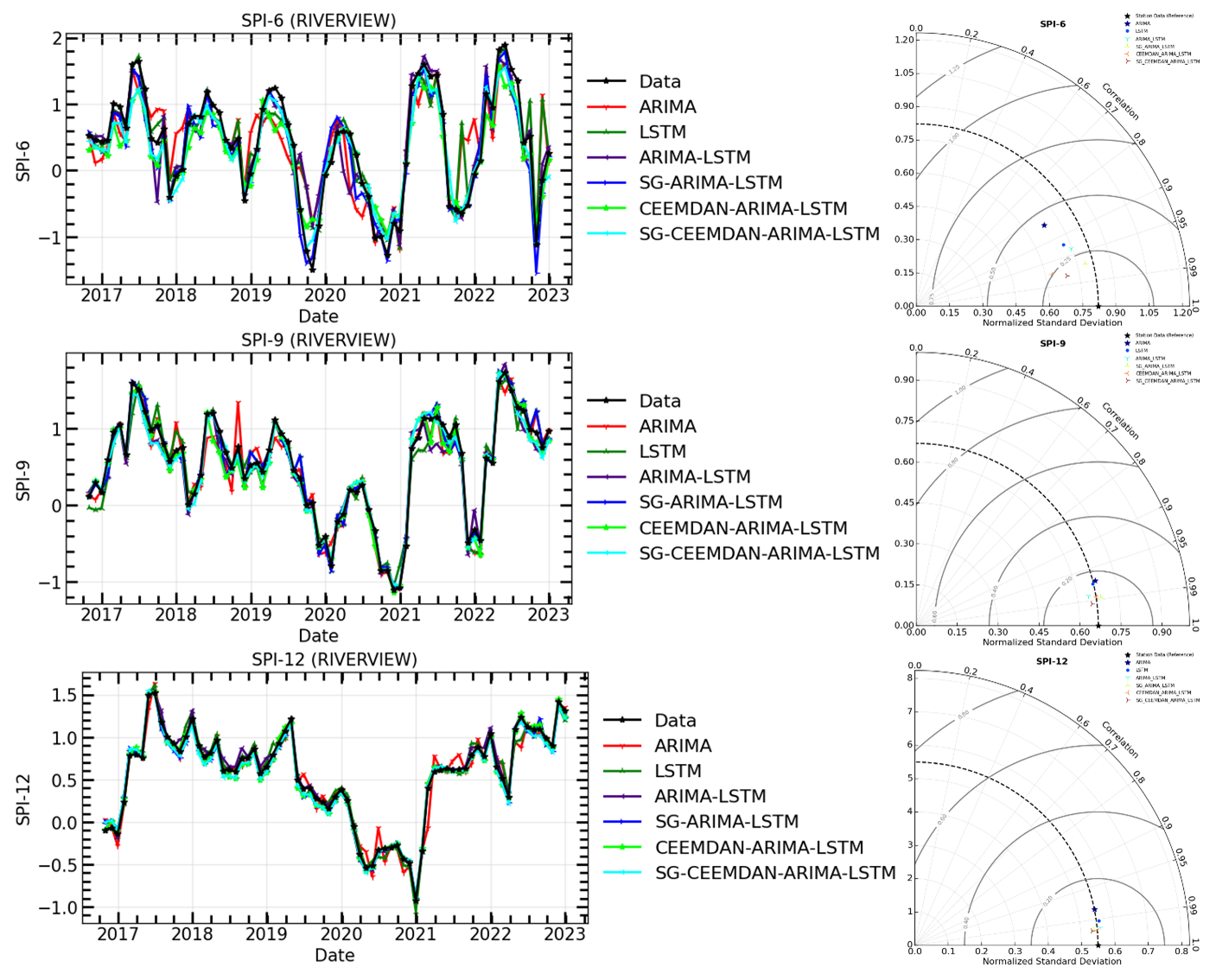
Figure 11 The time series of observations and hybrid forecasting models for SPI prediction (Left) and their Taylor diagram plots at different timescales (Right) for SPI-6, SPI-9, and SPI-12 of Riverview meteorological station.

In general, both Fig. 8 and Table 3 show that all stations, except Riverview, indicate a downward trend for all time scales, in terms of the ITA. For example, the ITA results obtained using 6-month SPI values exhibit a slightly decreasing trend in precipitation, moving toward the upper right quadrant, indicating the detection of drier conditions over the 6-month timescale. Some points approach the severely wet threshold but do not cross it, indicating that there were no extreme wet periods, though some drier periods are evident near the severe dry line. The ITA results obtained using 9-month SPI values show a more pronounced decreasing trend, indicating a relatively weaker increase in wet conditions over a 9-month timescale. Several points approach the severe dry threshold, but the data remains mostly within the 95 % confidence bounds, indicating moderate variability in precipitation trends. On the other hand, the SPI-12 plot demonstrates a noticeable decreasing trend toward dryness, as many points fall below the no-trend line and approach the severe dry region. Riverview indicates the increasing trend across all time scales. The increasing distance between the black dots and the no-trend line highlights a shift toward drier conditions in the second half of the series. In general, the analysis suggests a gradual increase in precipitation for shorter periods (SPI-6), moderate upward trends for medium-term periods (SPI-9), and a more substantial shift toward dry conditions over longer periods (SPI-12) for Riverview. The variability is evident, but a clear progression toward drier conditions is evident, particularly in the SPI-12 plot. This observation could be indicative of changing precipitation patterns, which is crucial for understanding drought risk and informing water resource management strategies.

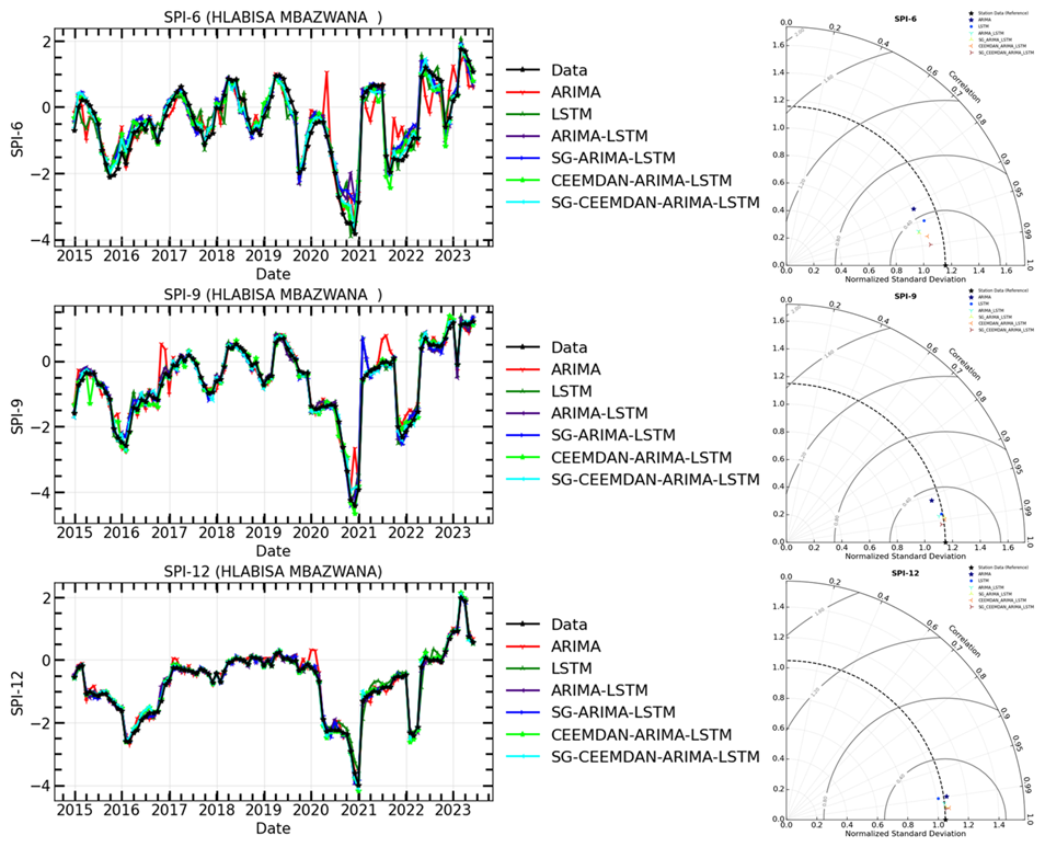
Figure 12 The time series of observations and hybrid forecasting models for SPI prediction (Left) and their Taylor diagram plots at different timescales (Right) for SPI-6, SPI-9, and SPI-12 of Hlabisa Mbazwana meteorological station.

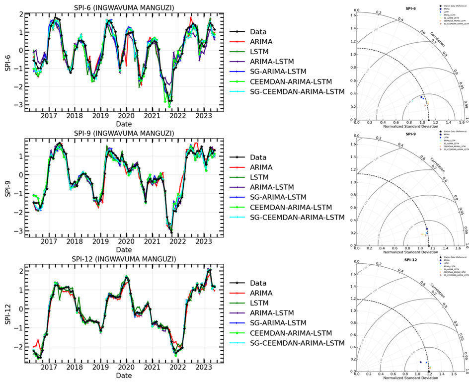
Figure 13 The time series of observations and hybrid forecasting models for SPI prediction (Left) and their Taylor diagram plots at different timescales (Right) for SPI-6, SPI-9, and SPI-12 of Ingwavuma Manguzi meteorological station.

Table 2 presents the results of the Mann-Kendall (MK) and Modified Mann-Kendall (MMK) trend tests for the Standardized Precipitation Index (SPI) over 6-month (SPI-6), 9-month (SPI-9), and 12-month (SPI-12) periods. The results indicate that across five stations all time scales both MK and MMK methods showed significant decreasing trend with negative Z-score values. For example, False Bay Park, Z_MK are $Z_{\text{SPI-6}}=-\mathrm{10.89}$, $Z_{\text{SPI-9}}=-\mathrm{12.89}$, $Z_{\text{SPI-12}}=-\mathrm{13.82}$ and Z_MMK are $Z_{\text{SPI-6}}=-\mathrm{6.27}$, $Z_{\text{SPI-9}}=-\mathrm{6.28}$, $Z_{\text{SPI-12}}=-\mathrm{6.29}$. The p-values of MK and MMK show the significance of the trends, with values way below 0.05 confirming statistically significant trends. In all cases except Riverview, the p-values are extremely low (≪0.05), indicating strong evidence of significant decreasing trends in precipitation for all SPI periods. Both the MK and MMK tests confirm decreasing trends across all time scales, with the Z_MK and Z_MMK values becoming more negative as the SPI period increases, reflecting an intensifying downward trend over longer periods (from SPI-6 to SPI-12). For Riverview station, the results indicate an increasing trend with positive Z-score values, i.e. Z_MK are Z_SPI-6=2.85, Z_SPI-9=3.84, Z_SPI-12=4.59 and Z_MMK are Z_SPI-6=1.19, Z_SPI-9=2.16, Z_SPI-12=2.29. In general, all these results are consistent with those shown using the ITA (see Table 3). The Riverview station experience increasing trend because it is located closer to the coast, hence it is influenced by a combination of geographic, oceanic and climatic factors. For an example, this station could be influenced by the Agulhas Current, which flows southwards along the east coast of South Africa, bringing warm, moist air from the Indian Ocean, and thus enhancing evaporation that brings constant availability of moisture in the atmosphere.

3.3 SPI Time Series Forecasting Results

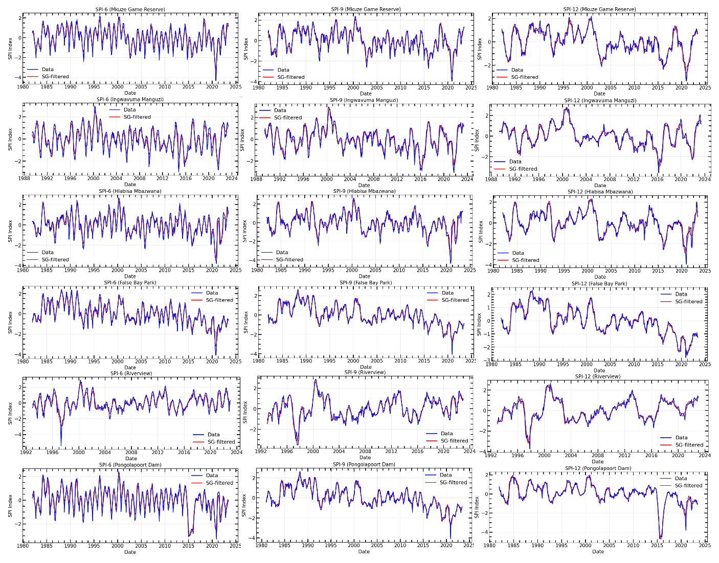
The study proposes a hybrid model that applies the Savitzky-Golay (SG) filter to process raw SPI data, thereby reducing noise and enhancing forecasting analysis. To demonstrate the effectiveness of the SG filter, appropriate parameters such as window size and polynomial order were selected through trial and error using data from the study sites (Sibiya et al., 2024). A window size of 21 and a polynomial order of 5 were chosen for smoothing. Figure 9 shows how the SG filter effectively tracks the general trend while preserving the shape of peaks and minimizing noise. This filter was applied to different time scales of the SPI time series. It autonomously calibrates according to peak distribution, exhibiting optimal performance, particularly with asymmetric peaks, while preserving peak height integrity. The application of the SG filter effectively mitigates short-term fluctuations and eliminates noise from the time series, resulting in cleaner data, thereby enhancing the reliability of the subsequent decomposition process. By reducing noise, decomposition techniques can more accurately capture the authentic underlying patterns and components within the data.

After applying a Savitzky-Golay filter to the series, the CEEMDAN algorithm decomposes the filtered SPI series into six subseries with different amplitudes and frequencies. The results from the False Bay Park station are utilized here as an illustration to prevent repetition. In these results, the decomposed set of time series consists of five IMF components and a residual component, as shown in Fig. 10 (for all time scales). During the decomposition process, white Gaussian noise is added to create noisy signals. The original sequence exhibits high nonlinearity and nonstationarity, with the frequency of the IMF components gradually decreasing. Figure 10 depicts this gradual decrease in frequency as the order of the IMF components increases. As each IMF is further decomposed, it becomes less volatile and cyclical, which aligns with the characteristics of the decomposed IMF. Therefore, by predicting each IMF and the residual, the forecast precision can be enhanced. A forecasting model is then constructed for each component, and the prediction results are obtained by summing up the outputs of all predicted components.

In predictive modeling, this study employed Bayesian optimization for hyperparameter tuning because of its effectiveness in improving model performance for complex, black-box, and non-differentiable functions. The hyperparameter configuration space comprises an n-dimensional functional space that encompasses all possible combinations of hyperparameters for the specified model. The benchmark analysis began with the ARIMA model, using the Box–Jenkins methodology. This process started with an assessment of stationarity through the augmented Dickey–Fuller (ADF) test. The series showed p-values exceeding the 5 % significance threshold, indicating non-stationarity (see Table 4). As a result, differencing was applied to achieve stationarity. This study employed a stepwise approach using the auto_arima(  ) function within the ARIMA framework to identify the optimal parameters (see Table 5). Table 6 delineates the hyperparameter search space employed for tuning the LSTM model utilizing a Bayesian optimization approach. Each hyperparameter is presented alongside its respective range or selected value, which delineates the parameters within which the Bayesian search investigated optimal configurations.

Table 5 Accuracy criteria for different model parameters of the ARIMA model applied in SPI-6, SPI-9 and SPI-12 at different meteorological stations of uMkhanyakude district.

Table 6 Hyperparameter ranges in LSTM–Bayesian search Method.

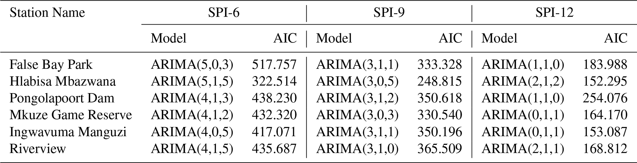
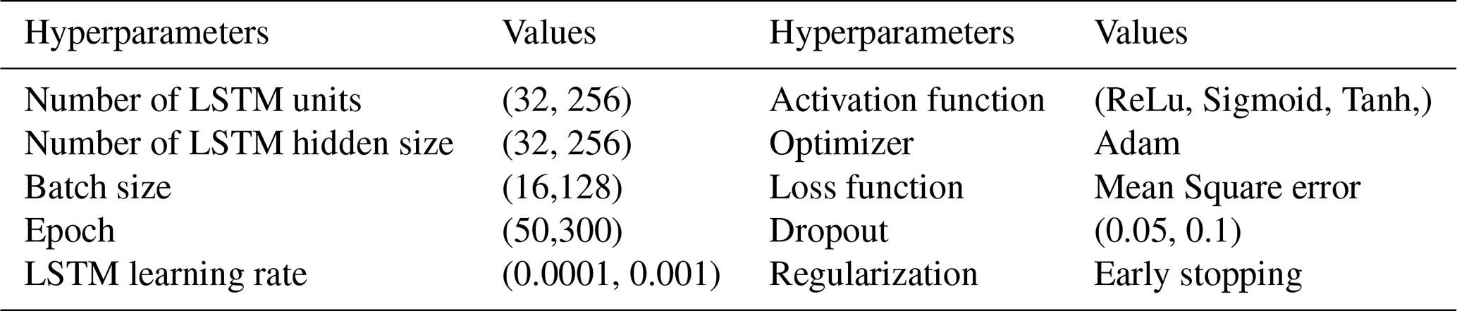
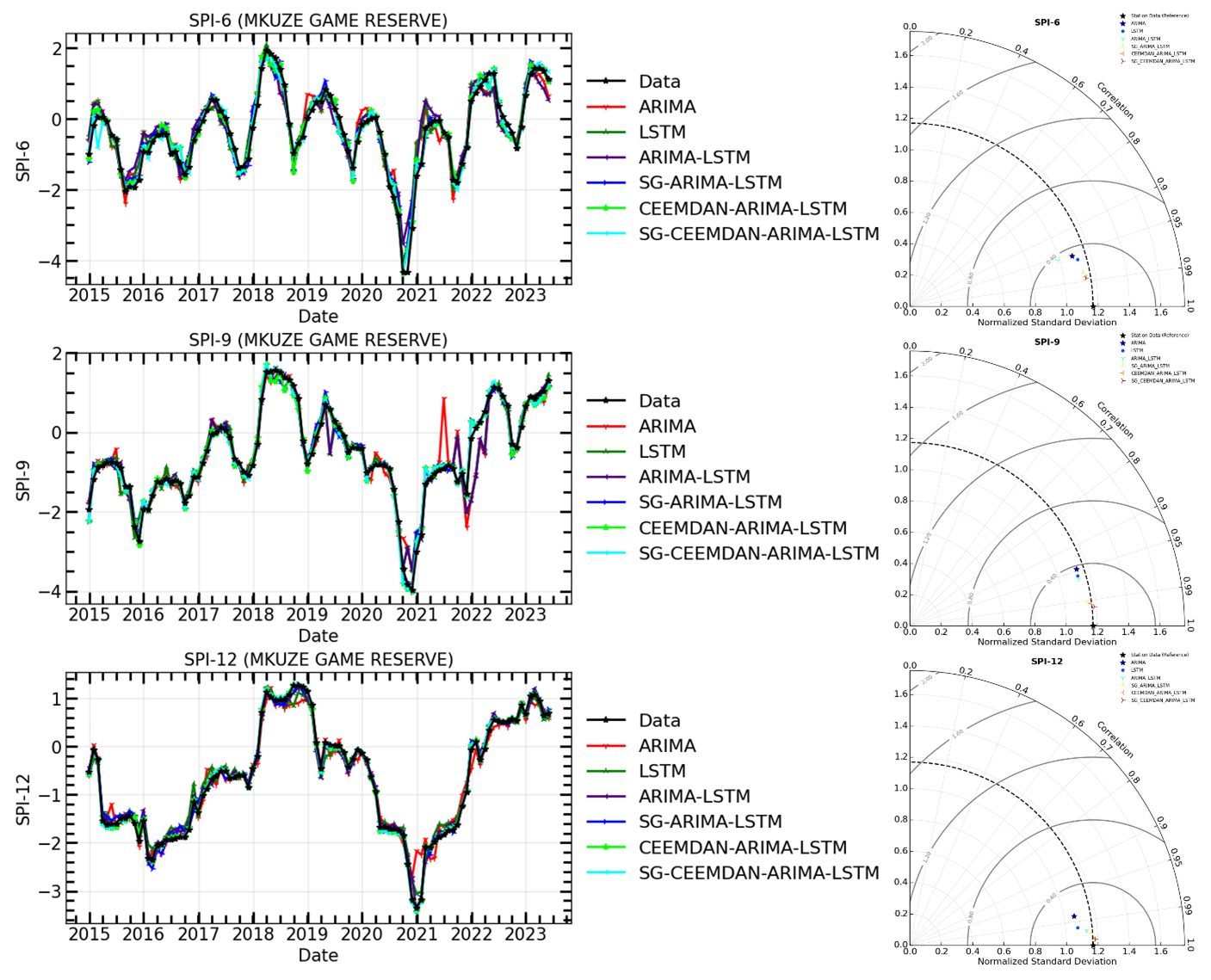
Figure 14 The time series of observations and hybrid forecasting models for SPI prediction (Left) and their Taylor diagram plots at different timescales (Right) for SPI-6, SPI-9, and SPI-12 of Mkuze Game Reserve meteorological station.

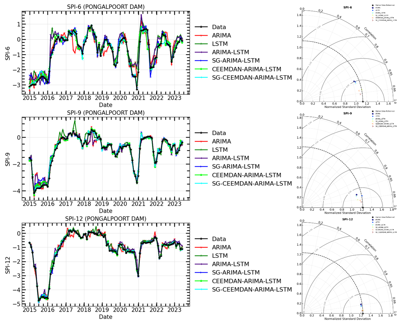
Figure 15 The time series of observations and hybrid forecasting models for SPI prediction (Left) and their Taylor diagram plots at different timescales (Right) for SPI-6, SPI-9, and SPI-12 of Pongolapoort dam meteorological station.

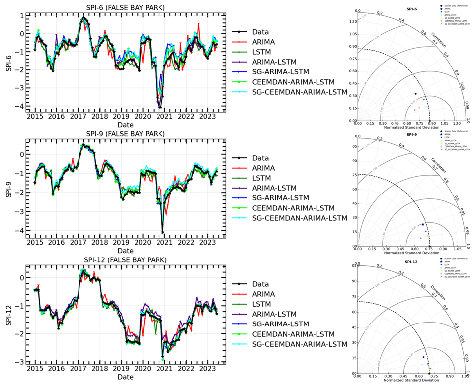
Figure 16 The time series of observations and hybrid forecasting models for SPI prediction (Left) and their Taylor diagram plots at different timescales (Right) for SPI-6, SPI-9, and SPI-12 of False Bay Park meteorological station.

The models in Table 7 were compared for their prediction ability before and after time series decomposition in this research. The objective was to determine if smoothing and decomposing time series improve the model's prediction performance. Figures 11–16 show a comparison of the various models' prediction outcomes using the Taylor diagram. In general, all the models accurately replicate the original SPI time series at all timescales (refer to Figs. 11–16) in terms of the time series plot. However, the SG-CEEMDAN-ARIMA-LSTM model (shown in red) appears to have the closest fit to the data, displaying superior accuracy across different phases, particularly in extreme values. Nonetheless, the hybrid models (SG-ARIMA-LSTM, CEEMDAN-ARIMA-LSTM, and SG-CEEMDAN-ARIMA-LSTM) show better precision in capturing peaks, rapid transitions and troughs compared to the standalone LSTM or ARIMA models. Table 7 displays an assessment of the predictive performance metrics of several models utilising RMSE, R², and DS. As the period extends, the RMSE values decrease; however, the DS and cap R-squared values typically enhance (see Table 7). This indicates that the models' predictive accuracy progressively enhances with an extended duration, reaching its highest point at the 12-month interval. In terms of RMSE, the SG-CEEMDAN-ARIMA-LSTM model outperforms the others, exhibiting the lowest error values across all indices. For example, Riverview station, 0.2165 for SPI-6, 0.0921 for SPI-9, and 0.0566 for SPI-12. This indicates that this model has the smallest prediction error, making it the most accurate in terms of error reduction. Concerning R², which measures how well the model explains the variance in the data, SG-CEEMDAN-ARIMA-LSTM again leads with the highest values: 0.9602 for SPI-6, 0.9846 for SPI-9, and 0.9939 for SPI-12. This shows that the model provides the best fit to the data. The CEEMDAN-ARIMA-LSTM model is the second-best performer, also exhibiting impressive results, particularly in R², where it achieves higher values of 0.9483 for SPI-6, 0.9751 for SPI-9, and 0.9933 for SPI-12. The SG-ARIMA-LSTM model is the third-best hybrid performer, with RMSE values of 0.2262 for SPI-6, 0.1051 for SPI-9, and 0.05639 for SPI-12. The SG-ARIMA-LSTM model is the third-best performer, also exhibiting impressive results, particularly in R², where it achieves higher values of 0.9392 for SPI-6, 0.9763 for SPI-9, and 0.9904 for SPI-12. The SG-ARIMA-LSTM model is the third-best hybrid performer, with RMSE values of 0.2597 for SPI-6, 0.1157 for SPI-9, and 0.0567 for SPI-12. In general, these results highlight the efficacy of hybrid models, particularly those incorporating SG and CEEMDAN processes, in improving predictive accuracy across multiple timescales of SPI, particularly for the SG-CEEMDAN-ARIMA-LSTM model. These results are consistent with the Taylor diagram (see Figs. 11–16), which indicates a significant improvement in prediction accuracy after incorporating the SG and CEEMDAN signal decomposition technique as the hybrid model exhibits superior performance in terms of prediction accuracy across all timescales, surpassing other models. This suggests that the inclusion of these techniques enhances the models' ability to capture both short-term and long-term dependencies, thus making them more robust for drought prediction purposes. Therefore, this hybrid model appears to be the most effective for drought prediction in this analysis. These findings highlight the superiority of the proposed hybrid model in enhancing drought prediction accuracy compared to standalone approaches.

Table 7 Performance measures for the comparison of observed and forecasted data of the models for SPI-6, SPI-9 and SPI-12 across various lead times using statistical criteria.

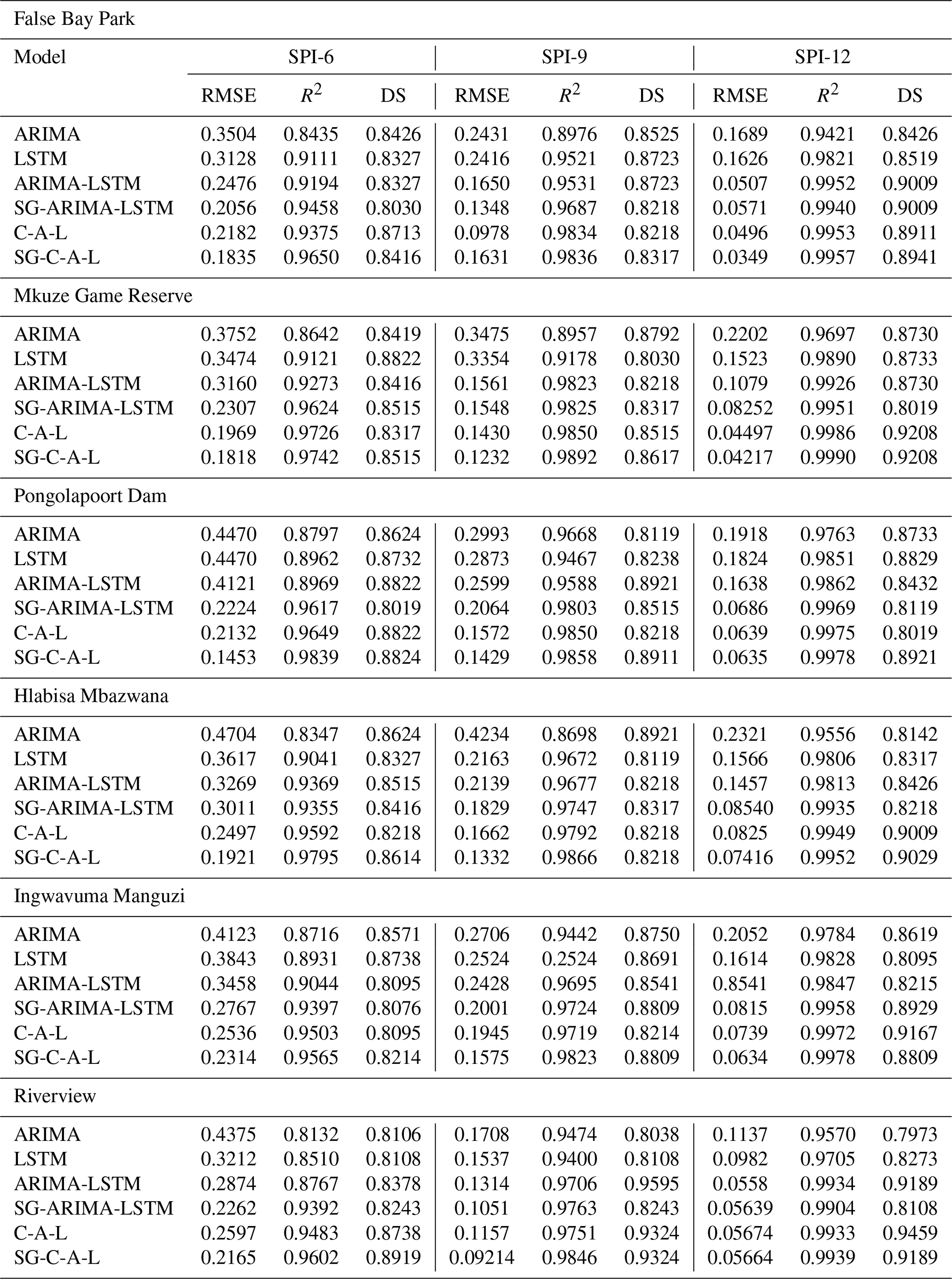
Note: C-A-L = CEEMDAN-ARIMA-LSTM.

4 Discussion

In this study, we utilized the Mann-Kendall and Modified Mann-Kendall tests to determine the drought trend index in meteorological variables within the basin. The MK and MMK trend methods showed a significant decrease in all SPI time scales based on rainfall data from five stations; however, the district, except for the Riverview station, showed an increasing trend in the uMkhanyakude district. The study's findings align with prior research by Kganvago et al. (2021) and Ngwenya et al. (2024). Ngwenya et al. (2024) conducted a study using the Mann-Kendall test to assess the SPI values at a 5 % significance level, revealing sustained drought conditions in the Western Cape region. Kganvago et al. (2021) indicated a notable decline in drought conditions in the Western Cape area of South Africa. We have also employed the ITA, which enhances the MK and MMK tests in identifying trends, and the results underscore the importance of comprehending drought conditions. The findings of our analysis validate previous research by Naik and Abiodun (2020), highlighting the need to conduct trend studies on drought indicators to investigate the impacts of climate change. The study highlights the crucial role of SPI as a primary variable in monitoring and forecasting droughts in the region, and its potential to mitigate the adverse impacts of droughts and water scarcity in the uMkhanyakude district in the future. The objective was to determine if the model's predictive performance is enhanced by smoothing and deconstructing time series data.

According to the statistical metrics in Table 7 and the Taylor diagram (see Figs. 11–16), the effectiveness of hybrid models that incorporate filter and signal decomposition techniques (SG and CEEMDAN) in improving prediction accuracy, particularly for drought forecasting, is highlighted. These findings support other research (Taylan et al., 2021; Elbeltagi et al., 2023; Rezaiy and Shabri, 2024), which highlights the superior accuracy of hybrid drought forecasting models compared to individual models. For example, Taylan et al. (2021) developed a hybrid model to forecast drought using precipitation data from Çanakkale, Gökçeada, and Bozcaada stations between 1975 and 2010. The study found that the hybrid models, which incorporated preprocessing techniques, performed better. Elbeltagi et al. (2023) utilized a hybrid model to estimate the SPI for 3, 6, and 12-month drought periods from 2000 to 2019. The findings demonstrated that RSS-M5P model yielded the most precise SPI predictions, with MAE =0.497, RMSE =0.682, RAE =81.88, RRSE =87.22, and R²=0.507 for SPI-3; MAE =0.452, RMSE =0.717, RAE =69.76, RRSE =85.24, and R²=0.402 for SPI-6 and MAE =0.294, RMSE =0.377, RAE = 55.79, RRSE =59.57, and R²=0.783 for SPI-12. The models employed to analyse drought in Jaisalmer, Rajasthan, yielded the most effective results, exceeding those of RSS-RF and RSS-RT. Additionally, Rezaiy and Shabri (2024b) introduced a W-EEMD-ARIMA model for drought prediction. This model utilises monthly precipitation data from Kabul spanning 1970 to 2019. The R² value was 0.9946, the MAPE was 18.9674, the RMSE was 0.0736, the MAE was 0.0575, and the SPI-12 validation indicated that our model was accurate. The outcomes obtained here surpassed those of the ARIMA, Wavelet-ARIMA, and EEMD-ARIMA models in terms of raw data (RMSE: 0.0858, MAE: 0.0660, MAPE: 24.5411, R²: 0.9925), analytical method (MAE: 0.1874, MAPE: 60.0220, R²: 0.9361), and maximum likelihood estimation (RMSE: 0.1002, MAE: 0.0691, MAPE: 23.7122, R²: 0.9898). During the SPI-3, SPI-6, and SPI-9 periods, our hybrid model consistently outperformed other models. Our proposed hybrid model surpasses ARIMA, Wavelet-ARIMA, and EEMD-ARIMA in enhancing the precision of drought predictions, as evidenced by this data.

In terms of term forecasting accuracy, the hybrid models, particularly SG-CEEMDAN-ARIMA-LSTM, consistently outperformed all other models across all SPI timescales, according to a comparison of this study's results with previous research. All models successfully reproduced the original SPI time series. With the range values of RMSE of 0.1453–0.2314 for SPI-6, 0.0921–0.1631 for SPI-9, and 0.0349–0.07416 for SPI-12, and the highest R² values of 0.9565–0.9839 for SPI-6, 0.9836–0.9892 for SPI-9, and 0.9939–0.9990 for SPI-12 across all timescales, the SG-CEEMDAN-ARIMA-LSTM model showed the most proficiency in capturing extreme values and rapid transitions. That these methods, when combined, improve the models' capacity to represent drought in the uMkhanyakude district, both in the short and long term, is supported by the data. This makes the models far better at foretelling when droughts will occur. In light of the foregoing, our study provides useful information regarding the use of the hybrid SG-CEEMDAN-ARIMA-LSTM model to the forecasting of meteorological droughts.

5 Conclusions

This study examined the trends in the Standardised Precipitation Index (SPI) over different timescales (SPI-6, SPI-9, and SPI-12) utilising the Mann-Kendall (MK), modified Mann-Kendall (MMK) test, and the innovative trend analysis (ITA) protocol. The monthly rainfall data from the uMkhanyakude district, South Africa, covering the years 1980 to 2023, was used for these calculations. Rainfall has been trending downward at a 95 % confidence level, according to the MK and MMK tests. The ITA results supported these findings as well, revealing a declining trend with most of the data points going below the 1:1 line. To predict SPI data over various timescales, this research employed LSTM and autoregressive integrated moving average (ARIMA) models. Researchers used a hybrid model that combines the SG-CEEMDAN processing method with the ARIMA-LSTM model to enhance the precision of SPI forecasts. They also used SG filtering and full ensemble empirical mode decomposition with adaptive noise (CEEMDAN). Figures 11–16 and Table 4 display the results of a thorough comparison examination of the forecast outcomes. The results revealed that the inclusion of preprocessing techniques (SG filtering, CEEMDAN, and SG-CEEMDAN) significantly improved the model performance in forecasting SPI at all timescales. The performance consistently increased with higher timescales, potentially due to lower noise levels. Across different timescales, the SG and CEEMDAN combined hybrid model consistently outperformed the individual models. Notably, the CEEMDAN-ARIMA-LSTM model outperformed the SG-ARIMA-LSTM model at all timescales, while the SG-CEEMDAN-ARIMA-LSTM model consistently exhibited the lowest root mean square error (RMSE) values across all indices. These results demonstrate that combining SG-CEEMDAN with ARIMA-LSTM has the potential to significantly enhance the accuracy of meteorological drought forecasting. The principal conclusion of the study is that ARIMA-LSTM, in conjunction with SG, CEEMDAN, and SG-CEEMDAN, serves as an effective instrument for early warning systems and meteorological drought prediction. The proposed methodology in this paper serves as a framework for modeling complex meteorological phenomena such as drought, which is particularly pertinent in semi-arid regions. Enhancing model performance and creating efficient models for weather forecasting can be achieved through techniques that address data noise, nonlinearity, and nonstationarity. To enhance water resource management, make informed decisions regarding agricultural output and tourism management, and establish regulations, it is essential to acquire extremely effective models for drought prediction. The omission of exogenous environmental variables in the SG-CEEMDAN-ARIMA-LSTM model represents a significant drawback of the study. The model's forecast accuracy and real-world application are limited by disregarding these exogenous effects, which can substantially affect drought conditions. Future studies should aim to include external variables, including temperature, soil moisture, vegetation indices, and anthropogenic factors such as land use and water management, to improve the model's efficacy. This integration would provide a more thorough comprehension of drought dynamics, hence improving the model's accuracy and dependability in drought predictions. Additionally, it is essential to investigate alternate decomposition methods, such as enhanced CEEMDAN (iCEEMDAN), which may provide significant insights.