Exploring seismic mass-movement data with anomaly detection and dynamic time warping

Catastrophic mass movements, such as rock avalanches, glacier collapses, and destructive debris flows, are typically rare events. Their detection is consequently challenging as annotated and verified events used as training data for instrumentation and algorithm tuning are absent or limited. In this work, we explore seismic mass-movement data through the lens of anomaly detection. The idea is to screen out segments of the data that are unlikely to contain mass movements by focusing only on anomalous signals, thereby reducing the number of signals to be studied, making downstream tasks such as expert labeling and clustering of events easier. To extract anomalous signals, we design a triggering algorithm using an anomaly score computed from an isolation forest obtained from sliding windows taken from the continuous data. The extracted signals are subjected to expert labeling and/or further analyzed by dynamic time warping, a popular technique used to evaluate the dissimilarity between different types of signals. We illustrate our approach by (a) mining for seismic signals of hazardous debris-flows in Switzerland's Illgraben catchment and (b) labeling of seismic mass movement data obtained from a Greenland seismometer network.

1 Introduction

Seismic networks record ground unrest and generate large amounts of continuous data in the public domain. Traditionally, global and regional earthquakes are the main focus of existing automated processing workflows by national and international seismological organizations. Event detection and arrival time picking for earthquake source location are consequently standard tasks, which until recently have required experts to manually classify seismic transients into earthquake-related signals or other types of events. Nowadays, however, machine learning takes over these processing routines facilitated by the existence of large manually labeled data volumes available for algorithm training (Woollam et al., 2022, and references therein). Machine learning algorithms can be trained with high-dimensional feature vectors and thus outperform conventional event detectors, like the short-term average over long-term average STA-LTA trigger (Allen, 1978), which operates on signal amplitude, only.

There exists a range of other important natural phenomena, whose seismic signatures often remain hidden in the vast amounts of available continuous data. Although there are ongoing efforts to detect and characterize non-earthquake seismic events (Bahavar et al., 2019), a big part of the available data remains unexplored. The topic of environmental seismology focuses on non-tectonic seismic events that are related to moving masses on the earth's surface (Larose et al., 2015). This includes catastrophic slope collapses in mountain regions (Allstadt et al., 2018), iceberg calving and resulting tsunami waves (Nettles and Ekström, 2010; Walter et al., 2013) as well as smaller events like rockfalls (Hibert et al., 2011), avalanches (van Herwijnen and Schweizer, 2011) and debris flows (Coviello et al., 2019), which nevertheless pose a threat to human lives and infrastructure. Seismometers can detect these events at kilometer distances and in case of the largest events even at hundreds of kilometers. Consequently, reliable detection is of high value for natural hazard research and monitoring.

Compared to earthquakes, the detection of mass movement signals in continuous seismic data is often more intricate: for events involving a granular mass, like avalanches and debris flows, seismic signals are generated by the chaotic superposition of particle-ground impacts (Zrelak et al., 2024, and references therein). This leads to emergent signals without identifiable seismic phases at frequencies above 1 Hz sustained over typical event durations on the minute scale (Provost et al., 2018). Iceberg calving signals are similar, although they also involve merging fractures and interaction with the proglacial water body (Bartholomaus et al., 2012). Events involving millions of cubic meters also produce seismic signals below 0.1 Hz as the bulk mass hinges over a contact point with the glacier terminus in the case of iceberg calving (Tsai et al., 2008) or accelerates along a runout trajectory in the case of slope failure (Ekström and Stark, 2013). In both cases, potentially impacted water bodies may resonate over many hours, which is often referred to as the “seiche” signal (Amundson et al., 2012; Walter et al., 2013; Svennevig et al., 2024).

For the emergent character of mass movement seismograms, statistical learning models have proven useful (Provost et al., 2017; Wenner et al., 2021; Chmiel et al., 2021; Zhou et al., 2025). In the presence of limited or no labels, unsupervised or semi-supervised methods are needed to create and refine catalogs of events (Meyer et al., 2019; Titos et al., 2025; Jiang et al., 2026). These types of analyses are challenging, due to high sampling rates (hundreds to thousands of Hertz) and the long-term measurements, spanning multiple years across multiple stations and networks.

From a data perspective, distinct physical seismic events like earthquakes or mass movements can be interpreted as anomalies in a background noise field. From a geophysical perspective, this background field is very complex, transient and non-stationary (Nakata et al., 2019; Fichtner et al., 2020) – so the term “noise” might be misleading for non-seismologists. Studying the properties of this seismic noise field has revolutionized passive seismology in the last decade, with applications ranging from global-scale subsurface tomography (Sager et al., 2020) to noise source location (Igel et al., 2021) and aquifer monitoring (Rodríguez Tribaldos and Ajo-Franklin, 2021). Compared to the duration of seismic signals from hazardous mass movements (minutes to hours), the rate of change in the background noise field throughout such events is often negligible, taking place on diurnal to seasonal time scales. This motivates us to tackle seismic signal detection from an anomaly detection approach.

Here we explore seismic mass-movement data by combining anomaly detection with semi- and unsupervised learning, using dynamic time warping (DTW) to quantify dissimilarity between signals. The idea is based on the insight that mass-movement signals represent significant statistical anomalies in the seismic data of instruments well-placed to detect these events. From this viewpoint, we should be able to screen out large portions of the data unlikely to contain mass movement signals, thereby reducing the number of signals to be studied. In this work, we consider the isolation forest (IF) algorithm, a classical yet powerful anomaly detection method. We chose this algorithm because of its favorable computational and memory complexity, strong empirical performance (Liu et al., 2008, 2012; Bouman et al., 2024) and minimal number of hyper-parameters to tune. Since unsupervised anomaly detection methods cannot discriminate between different types of anomalies, the extracted signals need to be further analyzed, either by expert labeling or unsupervised/semi-supervised methods. In this work, we pursue both approaches, the latter guided by measuring the dissimilarity between signals using DTW. To illustrate the value of our approach we consider refining an existing catalog of hazardous debris flows in Switzerland's Illgraben catchment, and generate a catalog from scratch for data obtained from a Greenland seismometer network.

2 Methodology

2.1 Preprocessing

We use the Scikit-learn (version 1.4.1) (Pedregosa et al., 2011) and ObsPy (version 1.4.0) (Beyreuther et al., 2010) libraries to implement the training and signal processing procedures. The preprocessing of the raw mini-seed seismic recordings follows standard procedures in seismology. In the first step, we identify gaps in the data and discard all recordings with less than 1000 consecutive samples, as gaps in the data indicate issues on the instrumentation side. We then apply a linear de-trending and de-meaning of each recording to ensure zero-mean recordings without a drift in amplitude, followed by a zero-phase high-pass filter with a corner frequency of 0.3 Hz. Furthermore, all data are re-sampled to the same sampling rate of 100 Hz. We refer to the units of the seismic waveforms after they have been preprocessed as preprocessed counts.

Table 1 Summary of terminology used for the different types of segments.

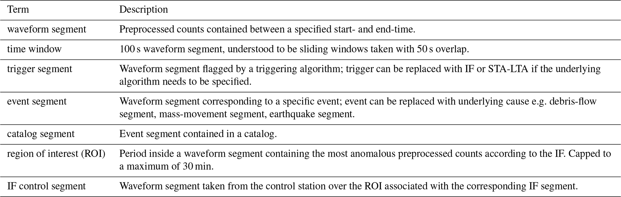
Fixed-size sliding windows have proven useful in converting time series data to a usable format for machine learning algorithms such as random forests, especially in the context of real-time monitoring (Wenner et al., 2021; Chmiel et al., 2021). We follow this convention by considering sliding windows covering 100 s periods taken with 50 s overlap. Generally, we denote the time series of preprocessed counts contained in a sliding window by bold x∈ℝ^T with T = 10 000, and refer to these as time windows for brevity. On the other hand, a waveform segment is characterized by a start- and end-time, and contains the time series of all the preprocessed counts observed over this period. We can take sliding windows over a waveform segment to generate a data set $\mathit{\{}{\mathit{x}}_{\mathrm{i}}:i=\mathrm{1},\mathrm{2},\mathrm{\dots },n\mathit{\}}$ of time windows which can be fed to a machine learning algorithm. If the waveform segment happens to contain time gaps, the sliding windows are taken separately over the contiguous components, and so n will depend on the length of the waveform segment alongside the number and size of the gaps.

In this work, we will refer to various types of waveform segments, which is described in Table 1 for reference. Additionally, to refer to the preprocessed count corresponding to time index t in a time window x we use the unbolded subscript x_t, while for an indexed time window x_i we use x_i,t.

2.2 Isolation forest

The intuition underlying the IF is that when anomalous observations are passed through randomized decision trees they tend to follow short paths to leaf nodes. By randomized decisions trees we mean that at each node a feature to split on is randomly selected, and a splitting point taken from the corresponding observed values in a subsample of the data, also at random. Such trees, which we refer to as isolation trees (iTrees) following Liu et al. (2008, 2012), are typically trained to a specified maximum depth or until a node contains a single observation. The IF itself consists of an ensemble of iTrees, trained on random subsamples of the data, which is used to compute anomaly scores of observations. Within the context of this paper, an observation corresponds to an entire time window and a splitting point to a specified preprocessed count.

We illustrate this intuition in Fig. 1 where we show how three time windows traverse through an iTree taken from the case study of Sect. 3.1. Two of these time windows were taken over a debris flow period and these require 1 and 3 splits, respectively to traverse to a leaf node. The third time window does not correspond to a debris flow and requires 8 splits to reach a leaf, which in this case equals the maximum depth parameter.

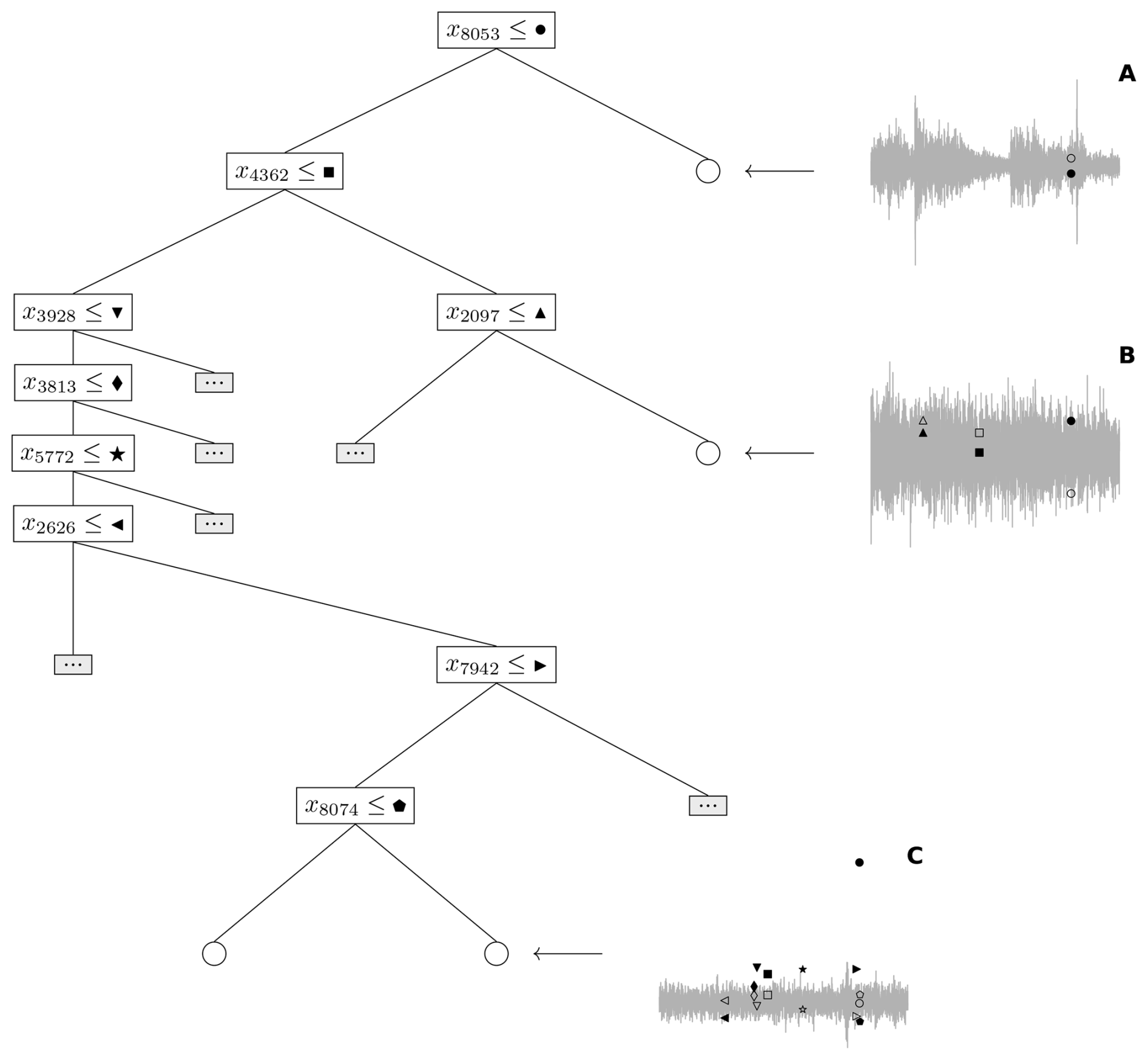
Figure 1 iTree trained to time windows from the waveform segment at ILL18 on 27 May 2018. The rectangular nodes show the preprocessed count represented by a filled marker and corresponding index used as a splitting point, while the circular nodes indicate leaf nodes. We show how three time windows traverse the iTree. The time windows displayed in panels (A) and (B) are taken from waveform segments corresponding to debris flows, while no debris-flow signal is present in the time window of panel (C). For each time window, the splitting points at the relevant time indices are shown alongside unfilled markers to indicate the corresponding preprocessed count of the time window. If the unfilled marker is above the filled one then the time window traverses to the right child of the corresponding node. We collapsed paths in the tree not relevant to the example time windows, these are represented by the small shaded rectangular nodes with ellipsis.

2.2.1 Training and evaluation

To each mini-seed seismic recording contained in a specified training period, we fit an iTree to the time windows extracted from the corresponding waveform segment so that the size of the IF ensemble corresponds to the number of mini-seed recordings. This was done so that the ensemble is representative of the entire training period under consideration. A specific iTree is trained on a random subsample of size ψ=256 taken from the time windows extracted over the corresponding miniseed recording to a maximum depth of log ₂(ψ)=8, so that the overall procedure has linear computational and memory complexity. This sub-sampling size was motivated empirically by Liu et al. (2008), and the choice of the maximum depth is the Scikit-learn default. We remark that a mini-seed recording typically corresponds to a calendar day and contains approximately 1728 time windows when taken with 50 s overlap. In the rare case that a recording do not contain 256 time windows, we upsample randomly with replacement so that the iTrees are always trained to subsamples of the same size.

The above choices can be appreciated via an analogy between the number of steps from root to terminal node for time window x in an iTree, and the path length of an unsuccessful search in a binary search tree (BST). For iTree r in an IF we denote the former by h_r(x) and refer to it as the path length for brevity. Assuming a random BST, the average path length of an unsuccessful search can be computed theoretically as $c\left(\mathit{\psi }\right)=\mathrm{2}H(\mathit{\psi }-\mathrm{1})-\frac{\mathrm{2}(\mathit{\psi }-\mathrm{1})}{\mathit{\psi }}$ with $H\left(j\right)\approx \log \left(j\right)+\mathit{\gamma }$ the harmonic number and γ Euler's constant (Liu et al., 2008). Because iTrees and binary search trees (BST) have an identical typology, c(ψ) serves as a reasonable reference value for the path length, although it is not necessarily true that 𝔼[h_r(x)]=c(ψ) for new time windows x not used to fit the iTree. Returning to Scikit-learn's default behavior, we observe that c(ψ)=𝒪(log ₂(ψ)) so that by default the maximum depth grows in the order of the average path length of an unsuccessful search in a random BST.

During evaluation, the iTrees are kept frozen and an IF anomaly score is computed for all time windows x extracted from the waveform segment covering the evaluation period. The more anomalous the time window x, the lower we expect the average of the path lengths $h\left(\mathit{x}\right)=\frac{\mathrm{1}}{R}{\sum }_{r=\mathrm{1}}^R{h}_{\mathrm{r}}\left(\mathit{x}\right)$ over the iTrees to be. The IF anomaly score for time window x is computed in Scikit-learn as

$$\begin{array}{}\text{(1)}& s\left(\mathit{x}\right)={\mathrm{2}}^{-\frac{\stackrel{\mathrm{̃}}{h}\left(\mathit{x}\right)}{c\left(\mathit{\psi }\right)}}\end{array}$$

where $\stackrel{\mathrm{̃}}{h}\left(\mathit{x}\right)=h\left(\mathit{x}\right)+\frac{\mathrm{1}}{R}{\sum }_{r=\mathrm{1}}^{R}c\left(n_{\mathrm{r}}\right(\mathit{x}\left)\right)$ with n_r(x) the number of time windows in the subsample used to construct iTree r in the corresponding leaf node of x. The additional term is a correction factor to account for the fact that the iTrees are not trained to their maximum granularity. We remark that $\mathrm{0}<s\left(\mathit{x}\right)<\mathrm{1}$ with a higher score indicating a more anomalous time window, and when s(x)=0.5 the corrected expected path length of x is equal to the BST reference value. Given that the iTrees are kept frozen, the evaluation has linear complexity in terms of the number of time windows.

2.2.2 Isolation forest trigger

Our objective is to find waveform segments in the seismic data containing counts that exhibit anomalous behavior. To this end we propose to use a trigger that operates on the IF anomaly scores of time windows, which we call the IF trigger. This trigger is activated when the IF anomaly score of a sliding window exceeds a specified onset threshold. We continue sliding windows until the IF anomaly score drops below a specified offset threshold, and we mark the waveform segment starting from the start time of the onset window until the start time of the offset window as anomalous. We refer to waveform segments flagged by the IF trigger as IF segments.

The onset and offset thresholds can be either preset or calibrated to annotations if available. In the case where calibration is not possible one needs to resort to rule-of-thumb values. While such recommendations are inherently heuristic in nature, we argue that such specifications should meet the following requirements:

1. An IF anomaly score of 0.5 means that the corrected average path length of the corresponding time window over the ensemble is equal to the BST reference value. Since approximately 11.42 % of all time windows considered in the case studies had an IF anomaly score of at least 0.5, this value should serve as a lower bound for both thresholds.

2. In the Case study of Sect. 3.2 there are several waveform segments corresponding to mass movements containing time windows with IF anomaly scores reaching values close to 0.7 (see Table B2) suggesting that this value should serve as an upper bound for both thresholds.

3. In cases where the IF anomaly score spikes briefly, having an offset threshold greater than the onset can lead to spuriously long IF segments, since we need to wait for the anomaly score to spike again above the offset threshold for the trigger to deactivate. To avoid such cases we require the onset threshold to be at least as large as the offset.

Our rule of thumb suggestion is to set the offset- and onset thresholds equal to 0.55 and 0.60, respectively. To further contextualize these choices, we show a quantile-function and histogram plot of all the IF anomaly scores computed in the case studies in Fig. 2. Around 5.05 % and 2.24 % of time windows had an IF anomaly score of at least 0.55 and 0.60, respectively.

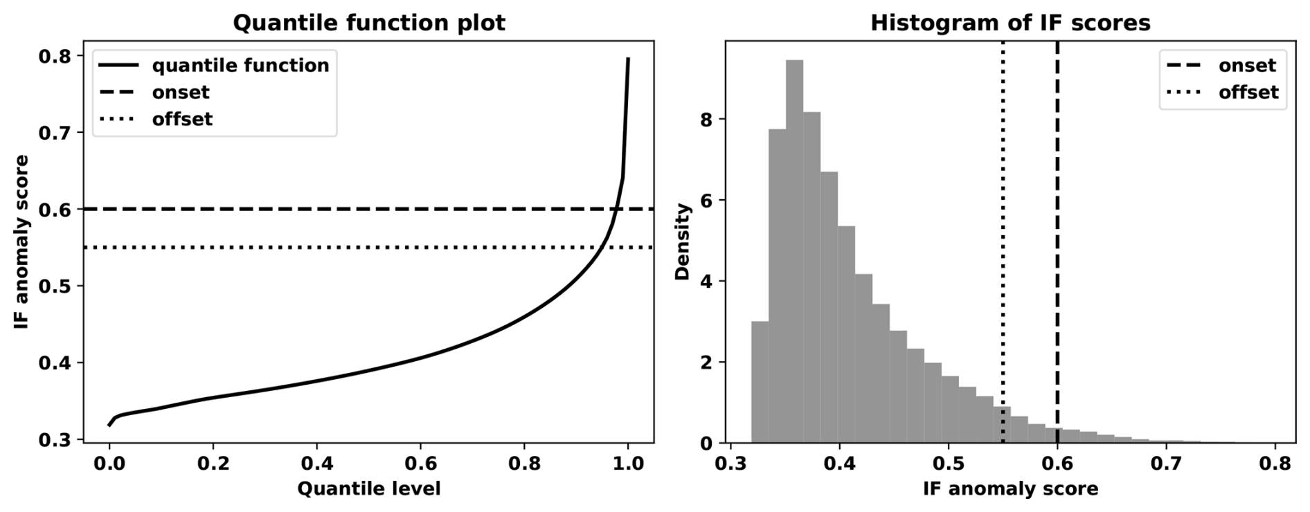
Figure 2 Quantile function plot and histogram of the IF anomaly scores computed for all time windows considered in the case studies.

To quantify the degree of anomalous behavior contained in an IF segment, we use the maximum IF anomaly score associated with the corresponding time windows and call this the IF segment score. This score can be used to propose a ranking of the IF segments for exploration purposes. We define the region of interest (ROI) of a waveform segment as the 30 min sub segment containing the most anomalous preprocessed counts; for segments shorter than 30 min, the ROI is the entire segment. In the case of waveform segments longer then 30 min, the ROI is extracted by identifying the time window with the highest IF anomaly score and iteratively expanding by adding the time window in the direction of the larger IF anomaly score, until the 30 min cap is reached.

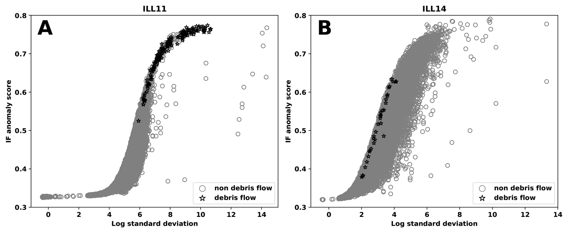
Figure 3 shows scatter plots of the IF anomaly scores against the log standard deviation of time windows observed at stations ILL11 and ILL14 during 2018 in the Illgraben seismic network considered in case study of Sect. 3.1. The scatter plots form a hook-like pattern with time windows related to debris flows ranked highly in terms of the IF anomaly score for fixed log standard deviation values of the seismogram amplitude. The figure suggests that the IF segment score can rank IF segments related to debris flows (or mass movements in general) highly in stations like ILL11, but this will not always be the case, as illustrated by the ILL14 scatter plot. For stations like the latter, additional tools are needed to improve the exploration procedure in both the semi-supervised and unsupervised setting. At the same time, Fig. 3 shows that time windows with higher seismic amplitudes (higher standard deviation) tend to have higher anomaly scores. However, highly anomalous debris flow segments are not associated with the largest standard deviation (in particular, for ILL14). This shows that anomaly is based on waveform information beyond the seismogram amplitudes.

Figure 3 Scatter plots of IF anomaly score against the log standard deviation of time windows observed at station ILL11 (A) and ILL14 (B) during 2018. Similar plots for the remaining stations are shown in Fig. A1.

2.3 Dynamic time warping

To improve exploration of the IF segments we consider measuring dissimilarity between waveform segments using dynamic time warping (DTW). In DTW we align two sequences by matching entries between them such that the overall distance between matched entries are minimized, subject to constraints on how matches can be made. We illustrate this procedure in Fig. 4 showing two time windows taken from debris flow segments from the Illgraben seismic network at station ILL18. Both time windows are normalized to zero mean and unit standard deviation with matched normalized preprocessed counts indicated by gray line segments. Note that the first and last entry of the top time window are matched with the first and last entry of the bottom, respectively, and none of the gray line segments cross. These illustrate the constraints on the way in which the entries of the sequences are allowed to be matched.

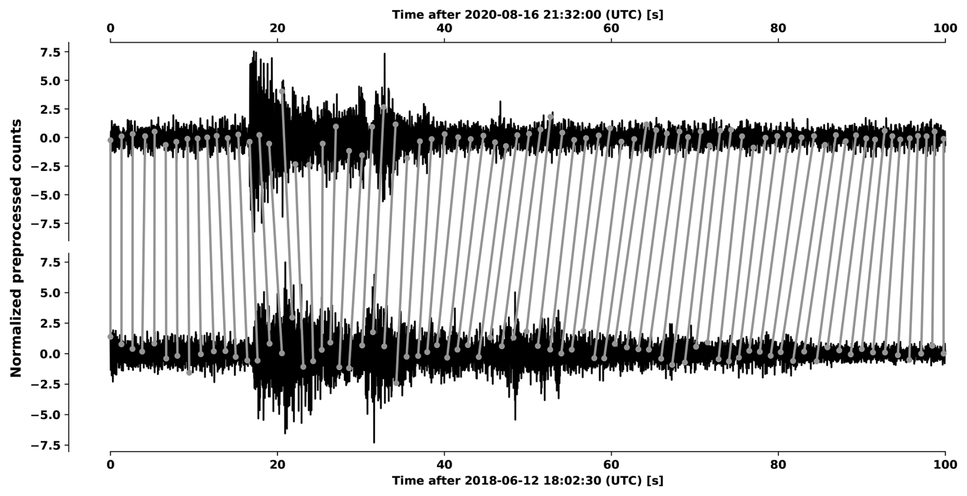
Figure 4 Illustration of DTW between two time windows taken from debris flow segments at station ILL18 of the Illgraben seismic network. To avoid unnecessary clutter, not all matches between the time windows are indicated.

More formally, suppose that we want to align two sequences ${\mathit{x}}_{\mathrm{1}}\in {\mathbb{R}}^{T_{\mathrm{1}}}$ and ${\mathit{x}}_{\mathrm{2}}\in {\mathbb{R}}^{T_{\mathrm{2}}}$, possibly of different lengths. We define a path $p=\mathit{\left\{}\right(i_k,j_k){\mathit{\}}}_{k=\mathrm{1}}^K$ such that $(i,j)\in p$ indicates that element i in x₁ has been matched with element j in x₂. We call a path p valid if it satisfies the following conditions:

1. $(i_{\mathrm{1}},j_{\mathrm{1}})=(\mathrm{1},\mathrm{1})$ and $(i_K,j_K)=(T_{\mathrm{1}},T_{\mathrm{2}})$.

2. $i_k\le i_{k+\mathrm{1}}\le i_k+\mathrm{1}$ and $j_k\le j_{k+\mathrm{1}}\le j_k+\mathrm{1}$.

The second condition ensures that the path respects the flow of time in both sequences; for example if we match element 3 in x₁ with element 10 in x₂ then we are not allowed to match element 20 in x₁ with element 2 in x₂ (this is why gray line segments in Fig. 4 do not cross). We remark that a valid path can contain repeated values with the interpretation of allowing local stretching/compression to align the sequences. The DTW objective is to find the valid path that minimizes the objective

$$\begin{array}{}\text{(2)}& \sum _{k}d(x_{\mathrm{1},i_k},x_{\mathrm{2},j_k}),\end{array}$$

where $d(\cdot ,\cdot )$ is a chosen distance metric such as the Euclidean distance. The minimizing path determines the DTW alignment between the sequences, and the corresponding value of Eq. (2) is called the DTW distance, although it does not define a proper metric since it does not necessarily satisfy the triangle inequality.

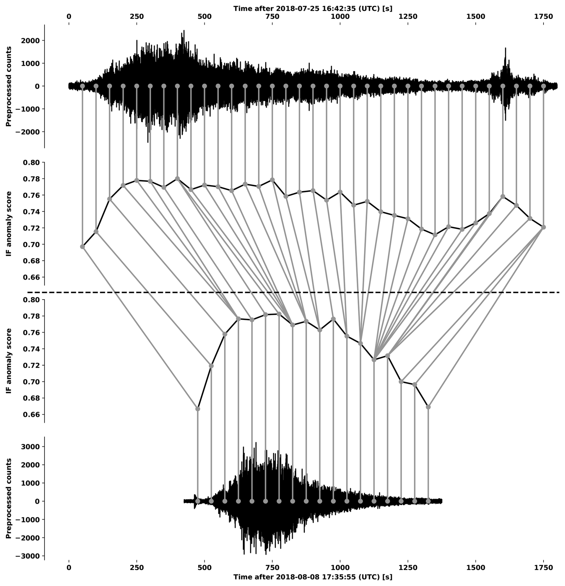
Figure 5 Illustration of segment DTW between two waveform segments corresponding to debris flows taken from station ILL18 in the Illgraben seismic network. The gray circles indicate the midpoints of time windows while the gray lines track the matching of time windows through the alignment of the IF anomaly scores.

The DTW problem can be solved using dynamic programming in 𝒪(T₁⋅T₂) time and storage complexity (Salvador and Chan, 2007). This does pose a computational bottleneck when comparing IF segments since such segments can span hours and therefore contain hundreds of thousands of preprocessed counts. In this work we address this bottleneck using a pre-alignment of time windows contained in segments as depicted in Fig. 5. The pre-alignment is done by extracting the time windows for each segment, computing the corresponding time series of IF anomaly scores and aligning them using DTW. Two time windows are matched if their corresponding anomaly scores were matched in the pre-alignment, and we compute the DTW distance between each pair of matched time windows. These distances are then aggregated into a single value using the median. We refer to this procedure as segment DTW and the corresponding median as the segment DTW distance.

We remark that in all cases time windows are normalized to zero mean and unit standard deviation before DTW is performed, and waveform segments are confined to their corresponding ROIs before application of segment DTW. The DTW alignment between time series of IF anomaly scores is done exactly, while the alignment between time windows is done approximately using the method of Salvador and Chan (2007) with a radius of 1.

2.4 Semi-supervised workflow

In the semi-supervised setting we assume access to an initial catalog of event segments that can be used to guide the exploration procedure in order to obtain a more complete catalog (see Fig. 6). We first split all available mini-seed recordings into a training- and testing period, the former used exclusively for calibrating the procedure. From the training mini-seed recordings we extract only those containing at least one initial catalog segment, and these recordings are used to calibrate a specified triggering algorithm. The calibrated trigger is applied to both the training- and testing recordings to flag segments in the data. These trigger segments are scored and subsequently ranked using a specified scoring method for the training- and testing periods separately. The calibrated trigger and scored segments remain frozen in subsequent updates of the catalog. A score threshold and minimum segment length are calibrated by comparing the trigger segments with segments contained in a specified calibration catalog over the training period. Trigger segments meeting the score threshold- and minimum segment length requirements become detections, separately for the training and testing periods. The detections are then subjected to expert labeling and used to produce an updated catalog. The calibration catalog is set to be the initial catalog during the first round of updates, and replaced with the updated catalog during subsequent ones. We also allow any of the initial catalog, calibration catalog and trigger segments to be pruned before any comparison to allow for the removal of waveform segments connected to an event with a specified degree of uncertainty.

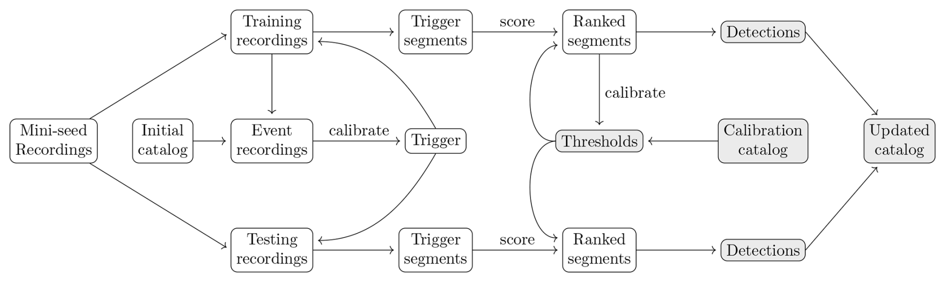
Figure 6 Exploration workflow in the semi-supervised case. The components that change following an update of the event catalog are indicated by shaded nodes.

For calibration purposes we compare a list of waveform segments to segments contained in a specified catalog using the intersection over union (IoU) metric. The IoU metric is defined to be the total time where the waveform segments in the list and catalog segments overlap expressed relative to the total time where either is present. In addition, we define a segment in the catalog to be a true positive if we can find at least one waveform segment in the list that overlaps with it, otherwise it is labeled a false negative. We define a true positive this way to avoid multiple counts of an event in the case where multiple waveform segments in the list overlap with it. If a waveform segment in the list does not overlap with any catalog segment, it is labeled a false positive. Using these definitions, we define

$$\begin{array}{ll}{\displaystyle }\text{recall}& {\displaystyle }={\displaystyle \frac{\text{TP}}{\text{TP}+\text{FP}}}\\ {\displaystyle }\text{precision}& {\displaystyle }={\displaystyle \frac{\text{TP}}{\text{TP}+\text{FN}}}.\end{array}$$

The recall therefore measures the proportion of catalog segments contained in a list of waveform segments, while precision measures the proportion of waveform segments in the list that intersect with catalog segments.

We consider three different versions of the semi-supervised workflow which we call the STA-LTA, IF and IF-DTW workflows. For the first we use the classical STA-LTA trigger where waveform segments are scored with the maximum value of the characteristic function over the corresponding period while for the second we use the IF trigger and score segments with the IF segment score. In the case of the IF-DTW workflow we again use the IF trigger but with an alternative scoring method using segment DTW. For this scoring method, we perform segment DTW between all pairs of initial catalog segments contained in the training period and use the pairwise segment DTW distances to construct a dendrogram under complete linkage. We then remove those initial catalog segments that do not form a sub cluster with other catalog segments before merging with the dendrogram (singleton merges), since such segments are considered unusual w.r.t. the majority of catalog segments according to the segment DTW distance. This procedure is illustrated in Fig. A2. An IF segment is then scored with the average segment DTW distance between the segment and the remaining initial catalog segments. If the IF segment happens to overlap with one of the remaining catalog segments, the corresponding segment DTW distance is excluded when computing the score.

2.5 Unsupervised workflow

In the unsupervised case we run the IF trigger using the rule of thumb thresholds and construct a clustering guided by the segment DTW distance. We found that performing pairwise segment DTW between a large number of IF segments to form a dendrogram can be computationally intractable due to the quadratic number of comparisons. In the case where the number of IF segments exceeds 200, we instead opted for an approach following Wu et al. (2018). The idea is to compute the segment DTW distances between an IF segment and a set of reference segments and use the corresponding distances as features to characterize the IF segments. Beyond the computational advantages, this approach yields a proper metric in the space of segment DTW distances and also allows additional features to be incorporated.

To find suitable reference segments, we first perform segment DTW between the leading 200 IF segments according to the IF segment score, construct a dendrogram using complete linkage, and cluster the segments using the Dynamic Hybrid cut method (Langfelder et al., 2007) with a deep split of 3 and minimum cluster size of 1. Inside each cluster we select the leading IF segment to use as a reference. We also included the IF segment score, length of the ROI and a feature describing the anomalous behavior of waveform segments at a control station over the ROI associated with the IF segments. The control station should be sufficiently far from the target station so that local events (in particular, mass movements) at the latter do not effect the former at the same time, and sufficiently close so that regional/global events (in particular, earthquakes) effect both stations at around the same time. The argument is that if we observe two high anomaly scores at both stations around the same time, this is likely caused by an earthquake rather than a mass movement. We define the IF control segment as the waveform segment taken from the control station over the ROI associated with the corresponding IF segment. Then we fit a new IF to the control station, and take the corresponding maximum IF anomaly score of the IF control segment as the control IF segment score.

To cluster the IF segments we performed min-max scaling of all the features followed by hierarchical clustering under Ward linkage. The Dynamic Hybrid cut method with a deep split of 3 and minimum cluster size of 10 was used to determine the clusters.

3 Case studies

We present two case studies for the application of the methodology described in Sect. 2. The first study aims to refine an existing catalog of debris flows in the Illgraben torrent, Switzerland, while the second focuses on generating a catalog of events from the seismic broadband station KARAT in Greenland. Overviews of these settings and maps of the respective seismic networks are provided in Fig. 7.

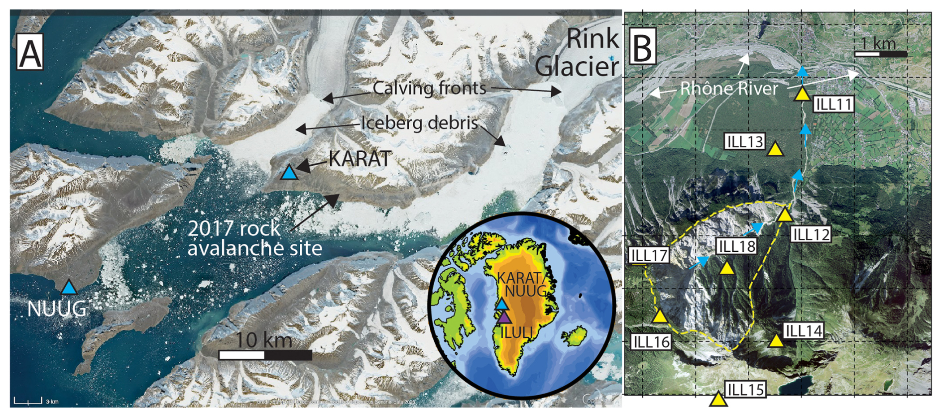
Figure 7 Study sites in Greenland (A) and Switzerland (B). (A) Karrat Fjord with seismic broadband stations (blue triangles), the location of the 2017 rock avalanche and major calving fronts indicated. White ice debris cover on the tidewater results from disintegrating icebergs. Inset shows the location of the site in Greenland. (B) Illgraben torrent with debris-flow-producing upper catchment outlined by yellow dashed lines. Blue arrows indicate flow direction. Yellow triangles represent seismometers. Sources: Copernicus (Sentinel-2 true color image) and inset using the Generic Mapping Toolbox and modified from Clinton et al. (2014) (A), Swisstopo (B).

3.1 Illgraben

3.1.1 Study site

Located in southern Switzerland's Canton Valais, the Illgraben is one of Europe's most active debris flow torrents. Its catchment drains an area of ca. 10 km² and produces sediments at higher elevation, which are mobilized during heavy precipitation to form debris flows and sediment-laden torrential floods. Each year, several such flows with volumes of a few tens of thousands m³ reach the Rhône River (Badoux et al., 2009; Hürlimann et al., 2003). Illgraben's debris flows move at several meters per second and feature the typical boulder-rich fronts, which are efficient seismic sources that can be detected on local seismic networks (Walter et al., 2017). At Illgraben, the Swiss Federal Institute for Forest, Snow and Landscape Research WSL maintains a semi-permanent seismic network that monitors debris flows and consists primarily of 1 Hz seismometers (Fig. 7). In addition, WSL's debris flow observatory at Illgraben contains geophone plates, automatic cameras and depth gauges to measure flow arrival times and flow depths at various points along the torrents, especially at concrete structures stabilizing the channel (“Check Dams”; Badoux et al., 2009). We consider data from the Illgraben seismic network for the period covering 10 April 2018 to 28 August 2022. Summary statistics are given in Table A1 of Appendix A3.

3.1.2 Debris-flow catalog

A debris flow signature can be defined to occur when the seismic waveforms of multiple stations are affected in the expected pattern as a debris flow moves down the torrent. This is illustrated in Fig. 8, where we show waveform segments and the corresponding IF anomaly scores on 6 July 2021 when a debris flow was active in the torrent. We see that the debris flow first effects the upper stations ILL14-ILL18 and subsequently ILL12, ILL13 and ILL11 in order.

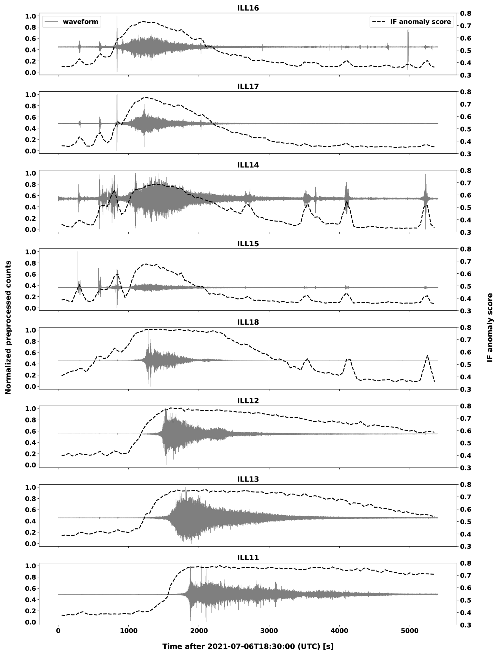
Figure 8 Time series plots of waveform segments and IF anomaly scores for stations in the Illgraben network from 6 July 2021 18:30:00 UTC to 6 July 2021 20:00:00 UTC. Preprocessed counts were normalized to the range [0,1] for each station. The IF anomaly tends to increase significantly before the visible onset of the debris flow particularly at stations ILL11 – ILL13 and ILL18. While this has not been systematically evaluated, we do not consider this early increase in the IF score to be attributable to the acausal filtering described in Sect. 2.1 since such preprocessing tends to suppress the amplitude of waveforms over debris flow events.

An existing catalog of debris flow segments, each coupled with a specific station, was independently curated by cross-referencing detections made by WSL's Illgraben debris flow observatory with the seismic waveforms of the stations in the network, keeping the above definition in mind. Since a debris flow signature does not always manifest as clearly as in Fig. 8, each debris flow segment in the catalog is associated with a confidence level, which is defined as follows:

1. High confidence. The segment is observed during a debris-flow signature and contains a clear signal.

2. Medium confidence. The segment is observed during a debris-flow signature and contains some signal, although somewhat suppressed. We also include here segments with a clear signal where not enough stations were active to establish if a debris-flow signature is present.

3. Low confidence. The segment is observed during a debris-flow signature; however, without the signature present in other stations it is debatable if this signal is related to a debris flow.

The existing catalog will be referred to as the WSL catalog with corresponding summary statistics given in Table A2 of Appendix A3. In the remainder of this section we refer to lower- and medium confidence segments in a catalog as lower-confidence segments. A trigger segment overlapping with a lower-confidence segment in a catalog, but with no high-confidence segment, is called a lower-confidence trigger segment.

3.1.3 Calibration

To each station in the Illgraben seismic network we apply the STA-LTA, IF and IF-DTW workflows of Sect. 2.4 using data from 2018–2020 for training. The calibration of the triggering algorithm for a station is done by using all corresponding segments in the WSL catalog as an initial catalog. The trigger segments are then extracted, scored and kept frozen. For the IF trigger, we select on- and offset thresholds from $\mathit{\{}\mathrm{0.55},\mathrm{0.6},\mathrm{0.65},\mathrm{0.7}\mathit{\}}$ and $\mathit{\{}\mathrm{0.50},\mathrm{0.55},\mathrm{0.6},\mathrm{0.65}\mathit{\}}$ through a grid search of the IoU metric, under the constraint that the onset threshold cannot be lower than the offset threshold. For the classical STA-LTA trigger, we found it difficult to choose a single grid that worked well on all stations and thus opted for a local search method instead. First, we conducted an extensive grid search on ILL11 and found that using a long-term window of 5000 s, a short-term window set to 10 % of the long-term window, and onset and offset thresholds of 6.0 and 0.125, respectively, yielded a high IoU score. This configuration of hyper-parameters was used as a starting point for all stations. We then performed local neighborhood searches, with an exponential step size of 2, until no improvement in the IoU metric can be found. The selected hyper parameters for both triggers are reported in Table A3.

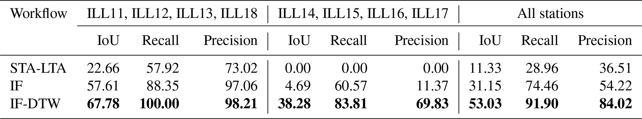
Table 2 Average metrics over different station groups during the test period from 2021–2022. All metrics are displayed as percentages rounded to two decimal places. The average metric of the best performing workflow is indicated in bold which in all cases is IF-DTW. We remark that when the STA-LTA workflow fails to make a detection over the test period at a specified station, the precision cannot be computed and in such cases we simply allocated a zero value to the metric.

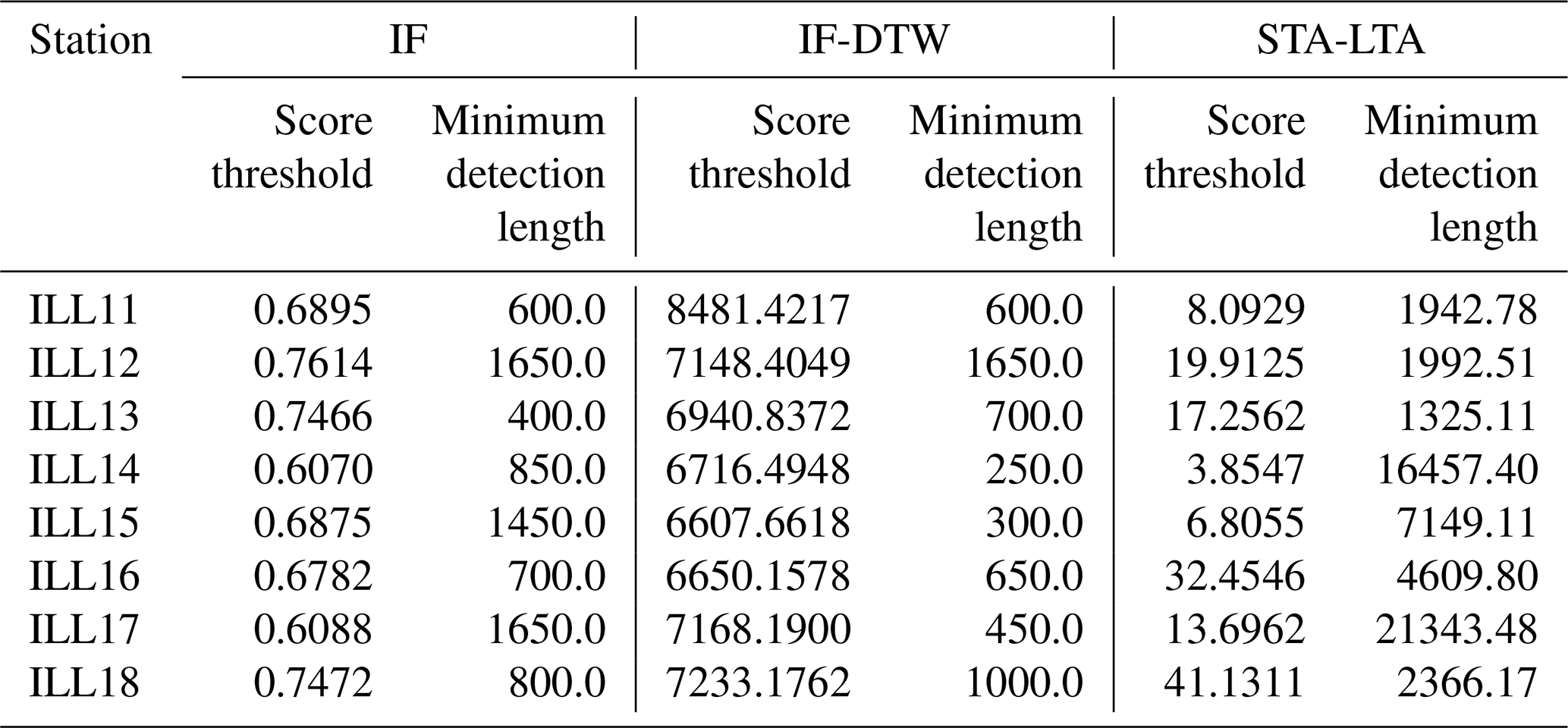
For calibration of the thresholds we used the catalog produced in the preprint version of this paper (Kamper et al., 2025). This catalog was produced following three major updates of the WSL catalog using the workflow of Fig. 6, but where a simpler form of DTW was used to score the segments. We provide more detail in Appendix A5, but note that after the second update in the formulation of this catalog the lower-confidence class was expanded to include other types of mass movements such as rockfalls, landslides and slope failures. For a chosen station we prune away lower-confidence catalog and trigger segments according to the preprint catalog before computing the IoU metric. In this way the lower-confidence segments are explicitly encouraged to be included in the trigger segments, and to become detections if they happen to be recovered alongside high-confidence segments. The selected score thresholds and minimum detection lengths for all the workflows are reported in Table A4.

3.1.4 Evaluation

Following the calibration procedure the detections made were used to update the preprint catalog and form a final evaluation catalog. In the formulation of this catalog, to keep the number of detections to investigate manageable, we excluded detections from stations ILL14, ILL15, ILL16 and ILL17 from the IF and STA-LTA workflows. These stations are located above Illgraben's upper catchment near substantial noise sources associated with a water reservoir, a skiing resort, cow grazing and human activity around various buildings. For IF-DTW, all detections were used to update the catalog. As in the calibration of the thresholds, for a given station, we prune away lower-confidence catalog segments and detections, this time according to the evaluation catalog. The corresponding pruned detections and catalog segments over a given time period are compared and used to calculate IoU, recall and precision metrics. We provide detailed tables of these values over the training and test periods in Tables A5 and A6, respectively, where the test period was taken to be 2021–2022. The respective number of low, medium and high confidence segments increased from 14, 23, 209 in the WSL catalog to 197, 44, 257 in the final updated catalog.

Table 2 provides average IoU, recall and precision metrics over the test period for three different station groups. The first station group containing stations ILL11, ILL12, ILL13 and ILL18 represents stations where the performance of all the methods is better relative to the second group, which contains stations ILL14, ILL15, ILL16 and ILL17. The third group corresponds to all the stations. With detection IoU, recall and precision of up to 68 %, 100 % and 98 %, respectively, we see that the IF-DTW outperforms the IF workflow. The IF workflow, in turn, outperforms the STA-LTA workflow in terms of the averages for all metrics and in all groups. While the performance of all methods are worse for the ILL14, ILL15, ILL16 and ILL17 station groups, the degradation is more severe for the STA-LTA and IF workflows.

We found that the STA-LTA trigger tends to prefer exceedingly long window sizes (see Table A3) to manage sensitivity towards amplitude, in order to avoid flagging an excessive number of false positive segments (see Fig. A3). However, these long window sizes lead to event masking, where a first event will suppress the characteristic function over a neighboring subsequent event inviting false negatives. We illustrate this in Fig. 9 where two debris flows segments associated with ILL18 on 31 July 2021 are shown. Due to the long window sizes, the characteristic function of the flows are suppressed by preceding increased amplitude in the seismic waveforms. We include more examples in Figs. A4 and A5.

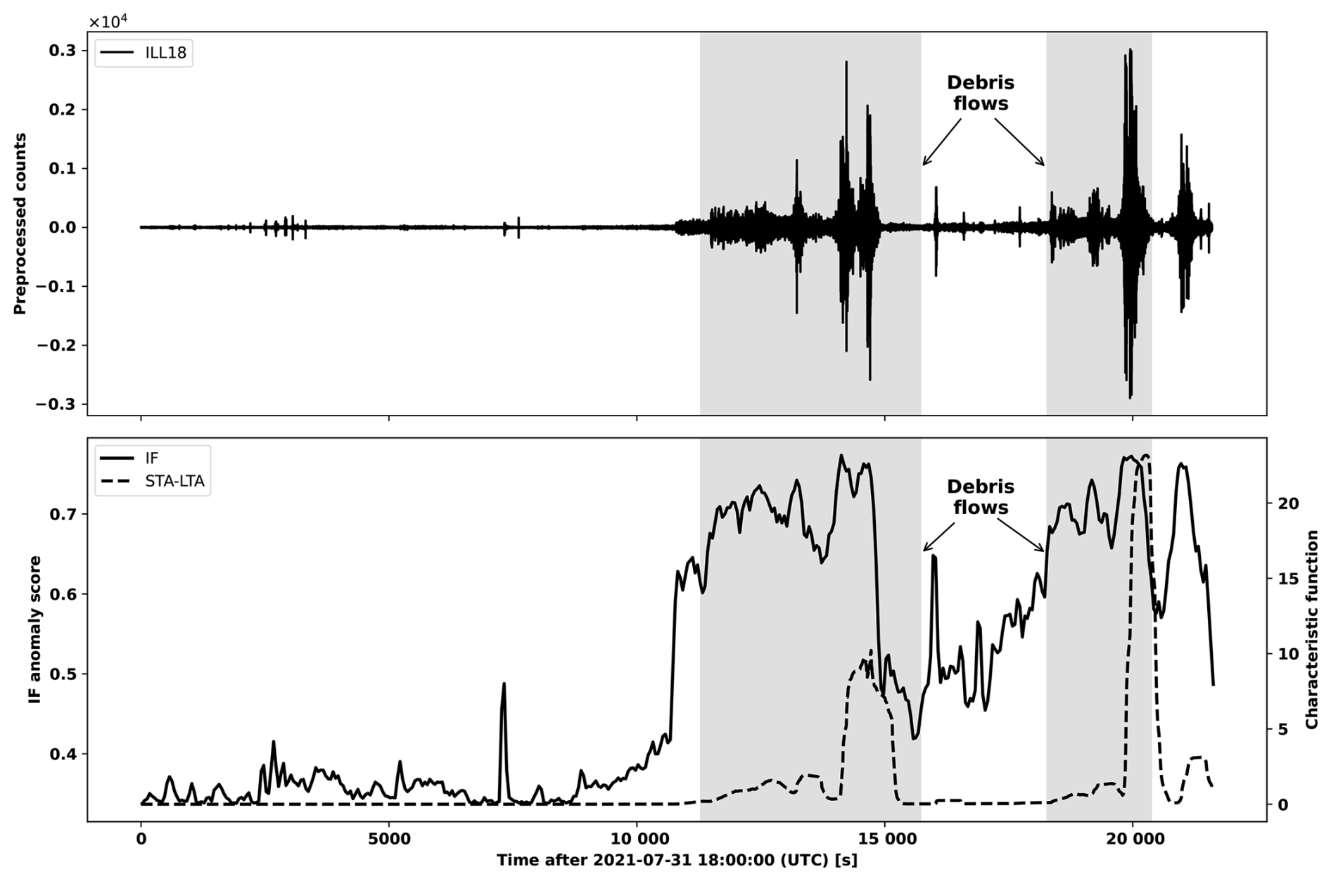
Figure 9 Illustration of the behavior of the STA-LTA characteristic function relative to the IF anomaly score at ILL18 on 31 July 2021. Debris flows are represented by the shaded regions.

The sensitivity of the STA-LTA trigger to amplitude and its proneness to event masking means that it is difficult to find a configuration of hyper parameters where both the number of false positives and false negatives are small. On the other hand, the IF anomaly score has a natural robustness to amplitude due to the threshold splits along the time axis used to construct iTrees (see Fig. 1). This is why the IF workflow provides superior metrics in terms of the IoU, recall and precision with an increase of 19.82 %, 45.50 % and 17.71 % on average for all stations over those produced by the STA-LTA workflow. We remark that since the IF anomaly score is computed from the path lengths in iTrees, which are built in a randomized manner, there is nothing explicitly guiding the score to discriminate between different types of events. This is in contrast to IF-DTW, where the score reflects the dissimilarity between the IF segment and debris flow segments according to the segment DTW distance. At stations ILL11–ILL13 and ILL18 the average improvement for the IoU, recall and precision metrics offered by the IF-DTW over the IF workflow is 10.17 %, 11.65 % and 1.15 %, respectively, and this increases to 33.59 %, 23.24 % and 58.46 % for stations ILL14–ILL17. The reason for the difference in the scale of the improvement is because the IF anomaly score happens to rank debris-flow time windows highly at stations ILL11-ILL13 and ILL18 (see Figs. 3 and A1).

3.2 Greenland

3.2.1 Study site

Our Greenlandic site locates on the western coast at the Karrat Fjord (Fig. 7). In this fjord system a 35–58 million  m³ rock avalanche occurred on 17 June 2017 generating a tsunami wave that destroyed parts of the nearby village Nuugaatsiaq and claimed 4 fatalities (Svennevig et al., 2020). The rock avalanche and precursory slip events left clear seismic signatures on the nearby broadband station NUUG, installed in the village Nuugaatsiaq (Poli, 2017; Seydoux et al., 2020). To investigate the detectability of the 17 June 2017 rock avalanche and comparable signals, we focus on station NUUG as well as KARAT, a broadband seismometer that was installed in summer 2022 about 6 km west of the rock avalanche epicenter. Finally, we also use the broadband station ILULI, which has been operating since 2009 in the village of Ilulissat, approximately 280 km south of Karrat Fjord.

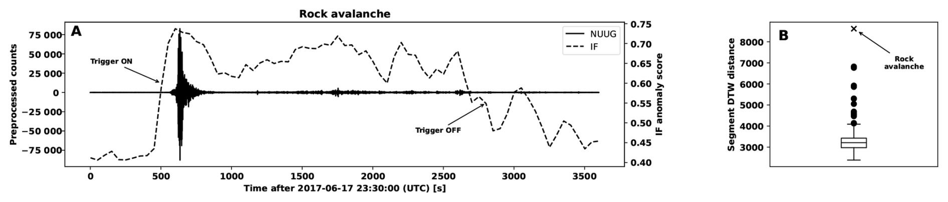
Figure 10 (A) Rock avalanche waveform segment observed at the NUUG station overlaid with the IF anomaly scores. (B) Boxplot of the heights at which individual IF segments merge with the remainder inside a dendrogram constructed from the pairwise segment DTW distances under complete linkage.

While our primary focus is the generation of a catalog of events for the KARAT station, we illustrate the unsupervised exploration procedure of Sect. 2.5 by applying it to waveforms obtained from NUUG over the period 1 January 2017 to 28 June 2017, using waveforms from ILULI over the period 1 January 2017 to 31 December 2017 as the control station (see Table B1 for summary statistics). The IF trigger flagged 194 segments in the corresponding waveforms. The highest ranking IF segment according to the IF segment score corresponds to the rock avalanche discussed in the preceding paragraph, with a corresponding value of 0.7373 and control IF segment score of 0.7171 (both accurate to four decimals). Time series of the preprocessed counts and IF anomaly scores contained in the rock avalanche segment are shown in Fig. 10. The same figure contains a boxplot of the heights at which individual IF segments merge with the remainder inside a dendrogram constructed from the pairwise segment DTW distances between the 194 IF segments under complete linkage. The larger the merge height, the more dissimilar the corresponding IF segment is with respect to the remaining segments. The rock avalanche segment achieved the largest height with a value of 8618.74. We emphasize that its enormous volume made this event a rare example of a mass movement that is strong enough to show up as a highly anomalous seismic signal at both NUUG and the control station ILULI.

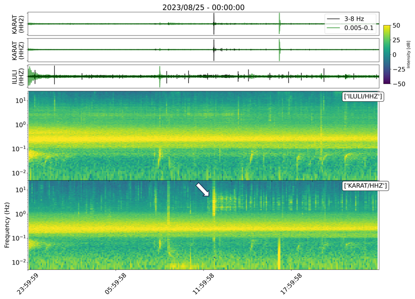
Figure 11 Seismic waveforms and corresponding spectrogram around the segment in cluster 8 flagged by the IF trigger on 25 August 2023. The IF trigger flags a typical calving seismogram.

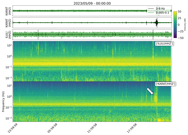
Figure 12 Seismic waveforms and corresponding spectrogram around the segment in cluster 9 flagged by the IF trigger on 9 May 2023. The IF trigger flags a typical calving seismogram.

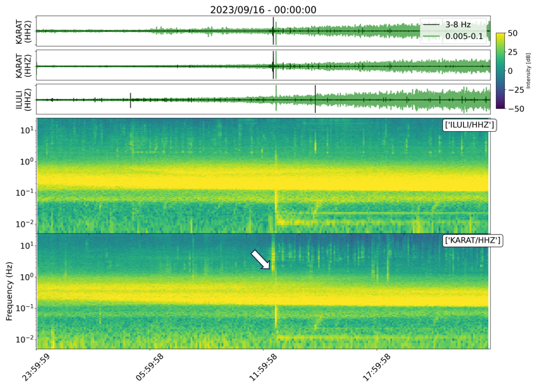
Figure 13 Seismic waveforms and corresponding spectrogram around the segment flagged in cluster 10 by the IF trigger on 16 September 2023 around the time when the Dixon fjord rock avalanche and tsunami occurred.

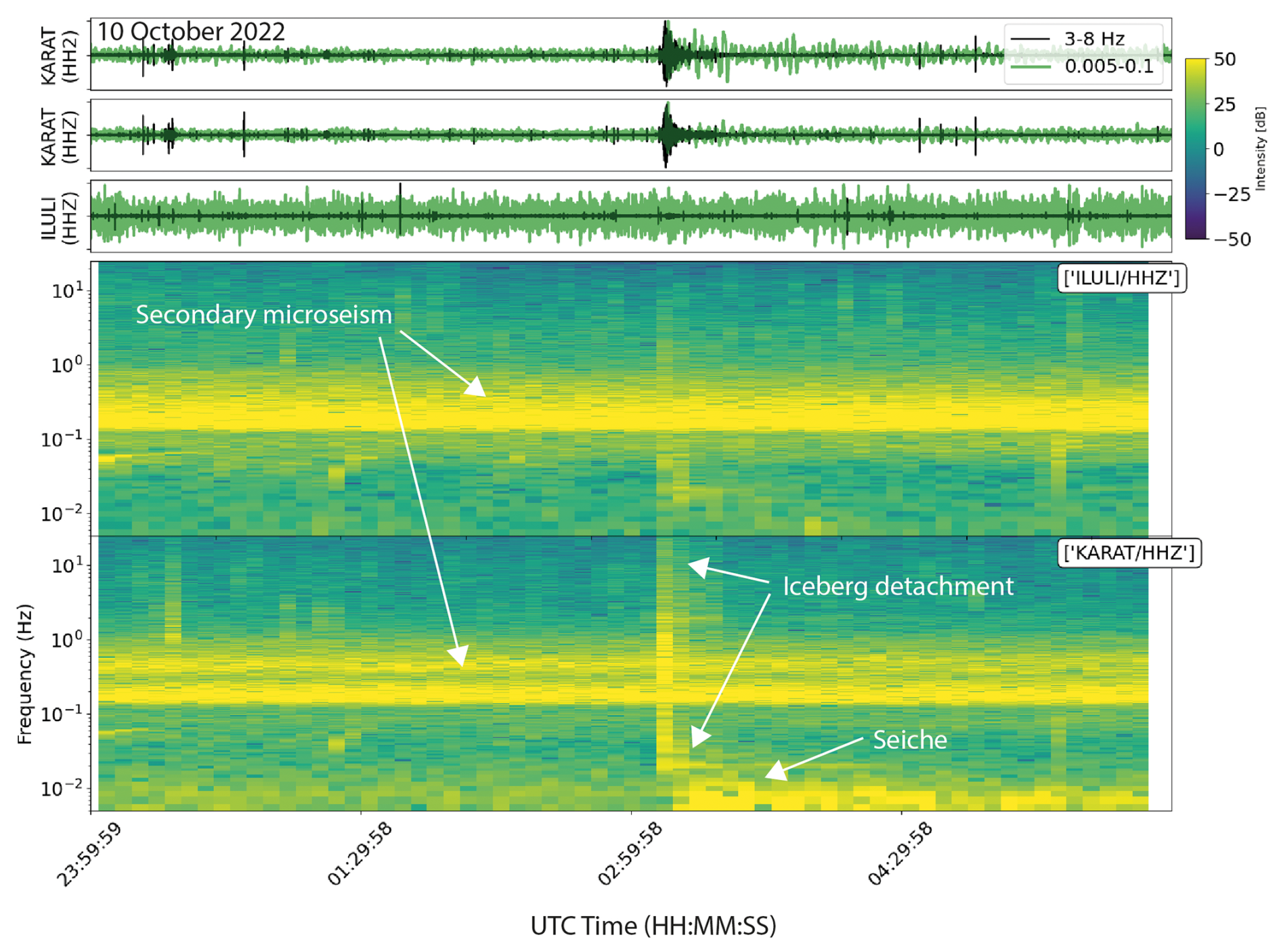
Figure 14 Seismic waveforms and corresponding spectrogram around the segment flagged in cluster 12 by the IF trigger on 10 October 2022 which according to satellite images constitutes a calving event (Fig. 15). One horizontal component (HH2) and the vertical component (HHZ) are shown for KARAT and the vertical component is shown for ILULI. The spectrograms show the continuous energy of the secondary microseism generated by standing waves in ocean basins (Longuet-Higgins, 1950; McNamara and Buland, 2004). The IF trigger flags a typical calving seismogram with broadband signals representing the iceberg detachment (Walter et al., 2012) and a low-frequency (< 0.01 Hz) signal generated by calving-induced water oscillations within the fjord (“seiche”; Amundson et al., 2012).

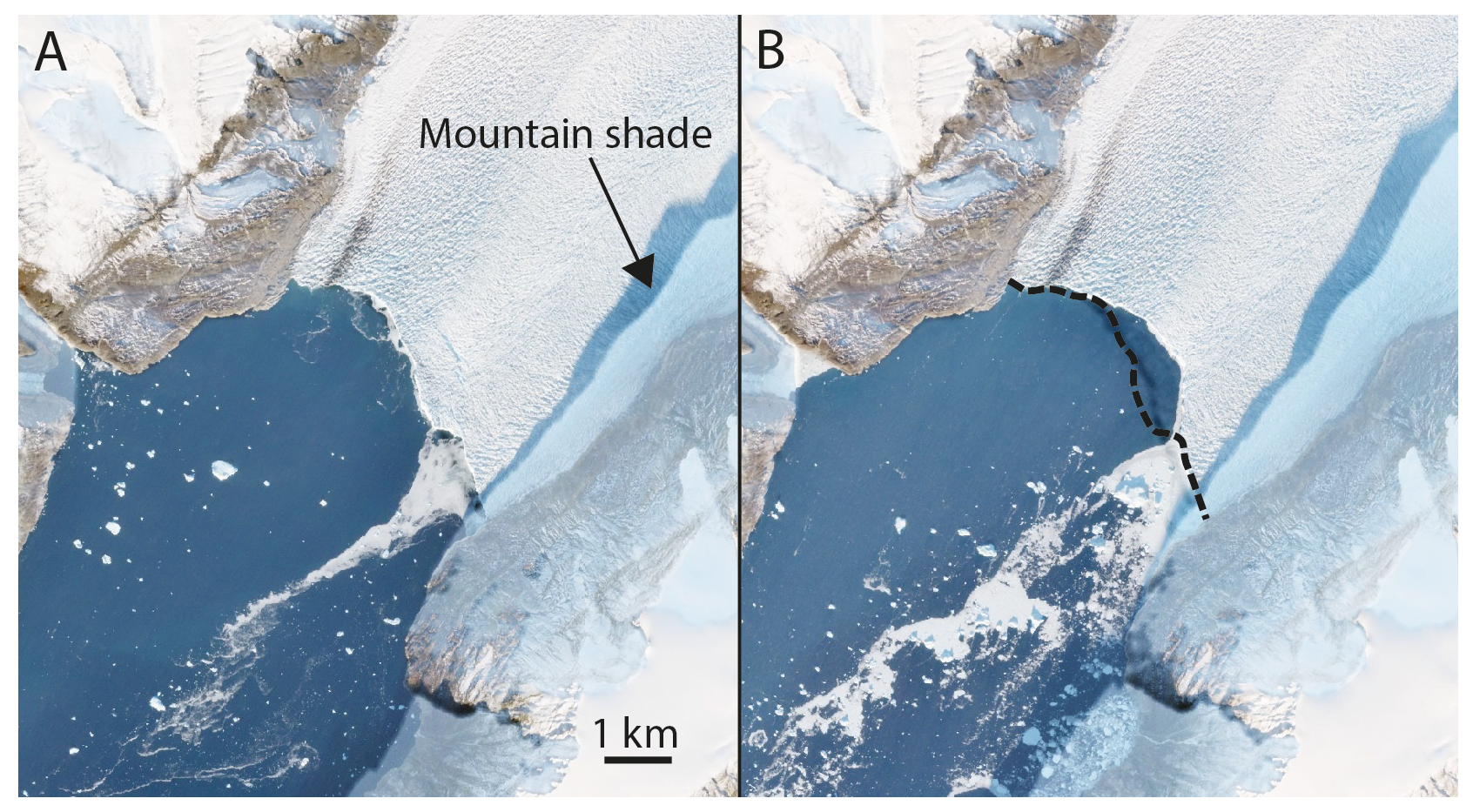
Figure 15 Satellite image pair of Rink Glacier calving front (Fig. 7) on 7 October 2022 (A) and 12 October 2022 (B) before and after the calving event 10 October 2022, respectively. The black dashed line represents the before-calving terminus and the missing area indicates a calving volume of about 0.5 km³ assuming a terminus thickness of 500–600 m (Medrzycka et al., 2016). Source: Sources: Copernicus (Sentinel-2 true color image).

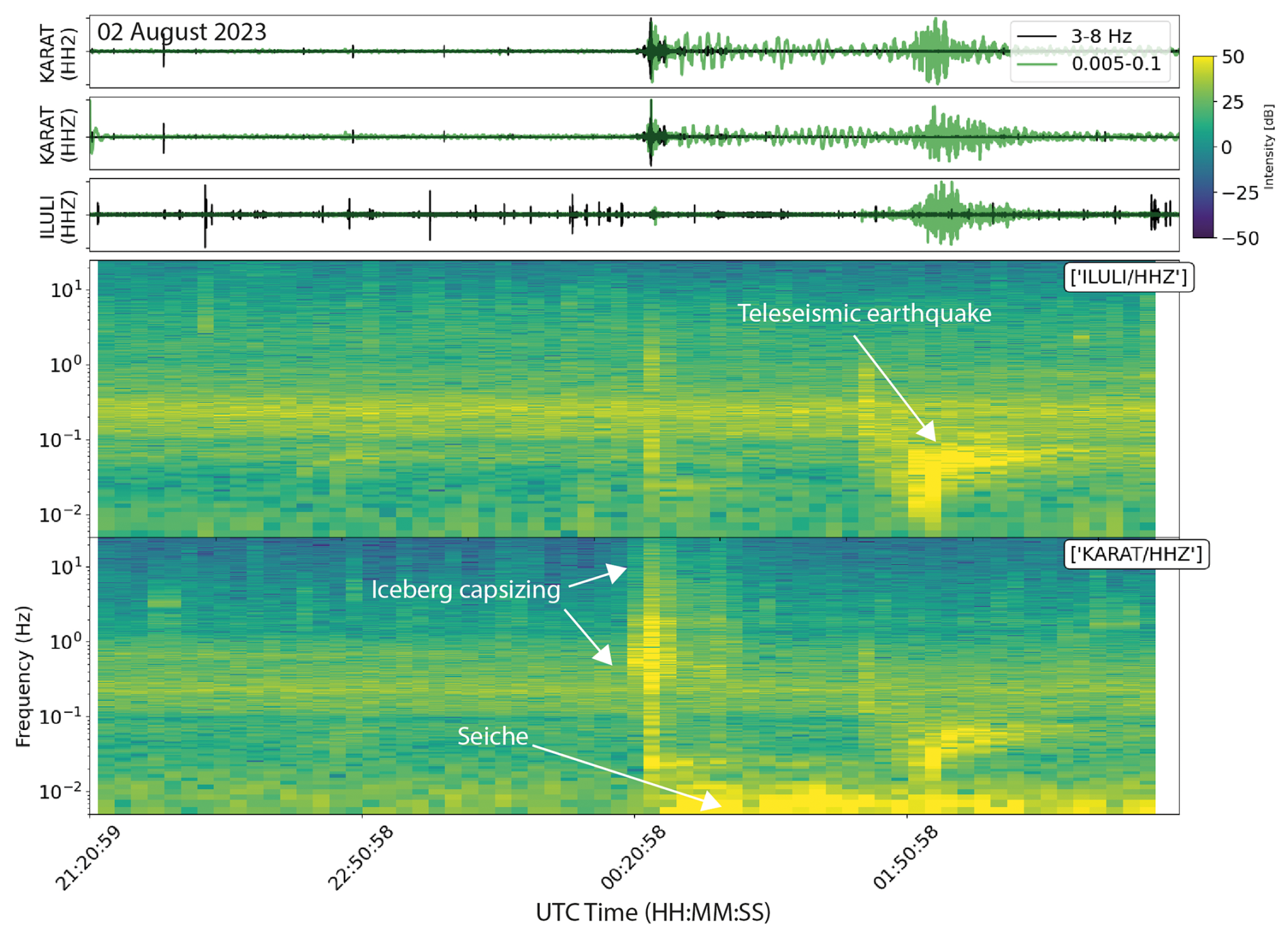
Figure 16 Seismic waveforms and corresponding spectrograms around the segment flagged in cluster 12 by the IF trigger on 3 August 2023, which according to satellite images constitutes the capsizing of a tabular iceberg (Fig. 17). The tabular iceberg was within 500 m of the calving front and thus likely contacted the calving front as it capsized. This generated a broadband signal similar to iceberg detachment (Fig. 14). Shortly after the capsizing, both KARAT and ILULI recorded a teleseismic earthquake (M 5.9, 266 km South of Burica, Panama, UTC time: 3 August 2023 01:25:21, location 5.640° N, 82.606° W) (U.S. Geological Survey, 2023).

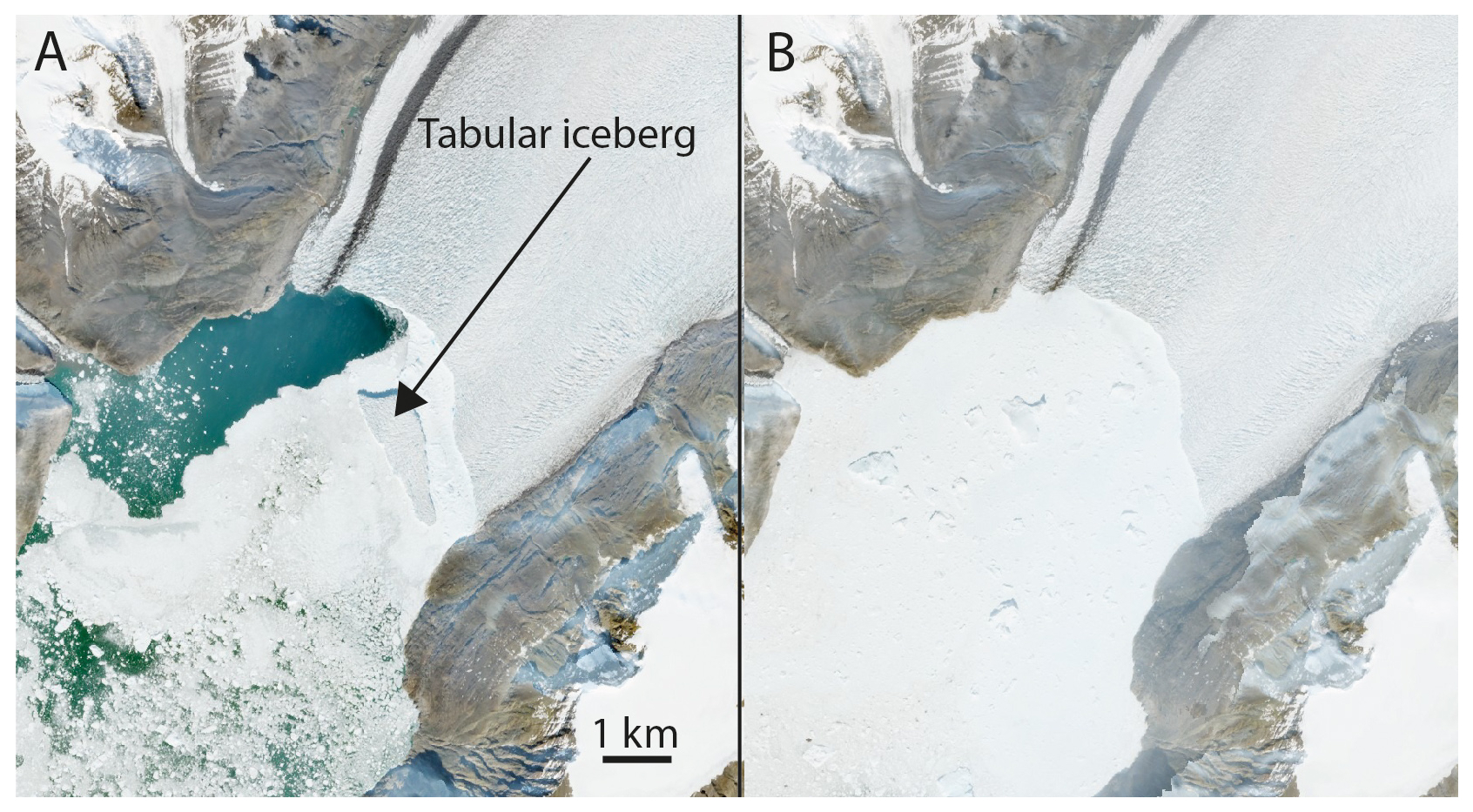
Figure 17 Satellite image pair of Rink Glacier calving front (Fig. 7) on 1 August 2023 (A) and 3 August 2023 (B) before and after the IF trigger segment on 3 August 2023, respectively. Assuming a full-thickness iceberg with a depth of 500–600 m (Medrzycka et al., 2016), the iceberg had a volume of about 0.5 km³ and may have contacted the terminus during capsize. Source: Copernicus (Sentinel-2 true color image).

3.2.2 KARAT clustering

We apply the exploration procedure of Sect. 2.5 to waveforms obtained from the KARAT station for the period 30 May 2022 to 20 October 2023 using waveforms from ILULI over the period 1 January 2022 to 31 December 2023 as the control station (see Table B1 for summary statistics). The IF trigger flagged a total of 605 segments in the KARAT waveforms of which we could relate 96 to mass movements, most of which are likely iceberg calving events. To determine if an IF segment is related to a mass movement the seismic waveforms and corresponding spectograms around the segment flagged by the IF trigger are investigated by a domain scientist and a mass-movement label is recommended based on well-known characteristics of calving seismograms (see Figs. 11–14 and 16). Once such a label is recommended, additional verification is performed using satellite images if available. A clearly missing piece of a glacier terminus confirms a calving event (Fig. 15). In some cases, the capsizing of a large tabular iceberg may produce a similar seismic signature (Fig. 17). An equivalent procedure is used to confirm whether an IF segment is related to a teleseismic or regional earthquake, with additional verification from the United States Geological Survey and the Geological Survey of Denmark and Greenland (U.S. Geological Survey, 2023; Geological Survey of Denmark and Greenland, 2025) earthquake catalogs. Fig. B2 shows for each $k\in \mathrm{1},\mathrm{2},\mathrm{\dots },\mathrm{605}$ the proportion of the k leading IF segments that are related to mass movements. The graph spikes fairly quickly with a maximum value of 45.83 % at k=48 showing that the IF segment score tends to rank mass movements highly.

Table 3 Summary of clusters from exploration procedure of Sect. 2.5 applied to the waveforms from the KARAT station. Shown are the membership percentages for the 4 categories. The tags EQ and MM stand for earthquakes and mass movements, respectively. The last column contains references to representative figures containing waveform-spectrogram plots for representative IF segments from chosen clusters. The bolded rows represent clusters in which we could find a relatively large number of mass-movement related IF segments.

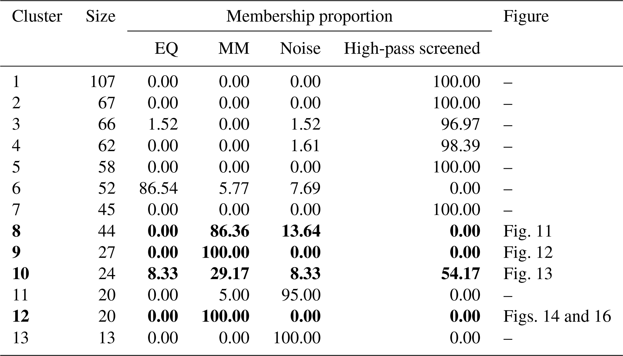
The unsupervised workflow split the 605 IF segments into 13 clusters as summarized in Table 3; the corresponding Ward linkage dendrogram and clustering of the IF segments are shown in Fig. B1. Cluster 13 is exclusively populated by highly ranked IF segments flagged before 15 August 2022 when the instrument was streaming sporadically and with high amplitudes (see Fig. B3). Since these likely correspond to issues on the instrumentation side, these segments are labeled as instrument-related noise. The noise class was expanded to include IF segments corresponding to anthropogenic events such as installation and service work near the station, helicopters arriving and departing from the station alongside electronic glitches/spikes. The majority of the IF segments in cluster 11 correspond to these events, with one IF segment possibly related to a mass movement, but with a degree of uncertainty. Around 29.91 % of the IF segments in cluster 1 were extracted from 25 and 26 September 2022, 2 d with 198 and 192 gaps in the corresponding recordings, so that spectrograms could not be computed. These segments contained unusually enhanced low-frequency (< 0.5 Hz) content. This was confirmed by observing that none of the IF segments inside the cluster survived a high-pass screening procedure whereby the raw waveforms over the IF segments are extracted, preprocessed by increasing the corner frequency of the zero-phase high-pass filter to 0.5 Hz and reapplying the IF trigger with no retraining. In the case of cluster 4, 95.16 % of the IF segments were extracted from 25 September 2022 and application of the high-pass screening process reduced the cluster to a single IF segment corresponding to noise. Similarly, we found that clusters 2, 3, 5, 7, 10 contain IF segments flagged due to increased low-frequency content, particularly during the months of September–January (see Fig. B3). Wind noise, ocean swell, snow cover and other meteorological conditions may explain this observation. Based on these findings, we explore a cluster only if at least one of the IF segments remaining after the high-pass screening can be related to a mass movement, otherwise the cluster is not explored further.

The results of the high-pass screening procedure left clusters 6, 8, 9, 10 and 12 to be inspected. Clusters 9 and 12 consisted of IF segments, which all resembled mass movements signatures. We give representative waveform-spectrogram plots of these clusters in Figs. 12, 14 and 16. Mass-movement related IF segments make up 86.36 % of cluster 8 which also contains a few noise related events; a representative example is given in Fig. 11. Cluster 10 consists of a number of exceedingly long IF segments with an average duration of 10.77 h. The the high-pass screening procedure left 14 IF segments, 10 of which are related to mass movements (some of the original IF segments are split into multiples by the high-pass screening). Included in the remaining IF segments is the Dixon fjord rock avalanche and tsunami (Svennevig et al., 2024) which is illustrated in Fig. 13. One of the remaining segments is related to a regional earthquake, another to a teleseismic earthquake and the remaining 2 to noise. The majority of the IF segments in cluster 6 correspond to earthquakes (86.54 %) alongside a few mass-movement- and noise related segments. One of these mass-movement events corresponds to a major calving event that occurred on 27 July 2023 and reached the ILULI station.

4 Summary, Conclusion and Outlook

We have showcased the ability of the IF trigger to flag mass movements in seismic waveforms to the degree that the method can be considered as an alternative to conventional algorithms when mining seismic data for such events. Applied to continuous seismic records from a debris flow catchment, our IF and STA-LTA triggers had been subjected to minimal preprocessing, and showed that the IF trigger can improve over the classical STA-LTA trigger up to 2.75 times in terms of the average IoU metric. The performance of both the IF and STA-LTA trigger could likely be improved by further data processing like band-pass filtering to focus on the most relevant frequencies. However, this requires prior knowledge as source-station distances affect peak frequencies of debris flow seismograms and background noise may pollute certain frequency bands, rendering them less suitable for seismic monitoring (Walter et al., 2017; Lai et al., 2018). It was the goal of this study to mine for mass movements without such prior knowledge, and our results show that in this sense the IF trigger is better suited than the STA-LTA trigger.

The potential of using DTW to measure dissimilarity between waveform segments for the purpose of mass-movement identification was illustrated in both a semi-supervised and unsupervised setting. In the case of the former, an improvement of 8.16 times in terms of the average IoU metric was observed over a pure IF workflow to explore for debris flows in the Illgraben catchment at selected stations.

Since reasonable mass movement detectors can be obtained at some stations just by thresholding the IF anomaly score, this score could serve as a useful feature when building more sophisticated classifiers in addition to those, for example, used in Chmiel et al. (2021); Zhou et al. (2025). Furthermore, running the IF trigger over a network of seismic stations can provide insights into how the network responds to mass movements and other events. Such insights could include (a) difficulty of detecting mass movements from different stations, (b) identification of other sources significantly affecting stations, and (c) examples of how these sources manifest in the seismic waveforms.

The isolation forest is a popular anomaly detection algorithm and has inspired many subsequent developments (Staerman et al., 2019; Cao et al., 2025). Notable extensions include the extended isolation forest (Hariri et al., 2021), deep isolation forest (Xu et al., 2023) and an IF variant that can identify anomalous subsequences in stationary time series data (Ting et al., 2024). Although identification of anomalous subsequences considered in the latter work aligns with our use of the isolation forest, the assumption of stationarity is too restrictive when considering seismic data. The extended isolation forest (EIF) has been shown to outperform the standard isolation forest in many applications (Bouman et al., 2024) and can serve as a ready-made replacement for IF in our applications. In the deep isolation forest data are fed through various randomly initialized multi-layer perceptrons (MLPs) and subsequently processed by classical IFs. By exchanging the MLP with other neural network architectures, dynamics related to how mass movements propagate through space and time can be encoded into the anomaly score which could improve corresponding detection. More broadly, alternative anomaly detection methods in the time series domain can be explored as reasonable alternatives to isolation-based methods (Blázquez-García et al., 2021; Schmidl et al., 2022; Herzen et al., 2022; Liu and Paparrizos, 2024). Features describing the anomalous behavior of waveform segments have been used as part of feature sets for supervised learning in seismological studies (Dempsey et al., 2020; Zhou et al., 2024, 2025). We remark that such feature sets and others used in a similar context (Chmiel et al., 2021; Zhou et al., 2025) can be processed through the isolation forest to produce an anomaly score. In this work, since our objective is exploration, we did not commit to a specific feature set and chose to work directly with the waveforms.

The use of DTW for waveform searching over cross correlation was suggested by Kumar et al. (2022) and the DTW distance matrix used as a basis for k-means clustering of waveform segments by Ida et al. (2022). In the case of the latter, 90 waveform segments were manually extracted over a 10 h period and provided to the clustering algorithm. Since the extracted waveform segments spanned periods of 2–7 s, the computation of the pairwise DTW distances is computationally feasible. We did explore performing exact DTW between aggregated values of time windows, including time series of the IF anomaly scores and principal component (PCA) projections, but this degraded the performance of exploration procedures. Alternatively, DTW can be applied in a multivariate context to time series features of time windows as discussed in the preceding paragraph or inspiration can be draw from application of DTW in the audio domain (Sakoe and Chiba, 1978). More ambitiously, self-supervised neural network approaches (Franceschi et al., 2019; Yue et al., 2022) or contrastive learning in the presence if weakly labeled data (Meyer et al., 2021) can be used to learn features of waveform segments either to apply DTW to, or use directly in a clustering or semi-supervised procedure. Approximate differentiable DTW distance functions (Cuturi and Blondel, 2017) can be incorporated into neural network architectures to learn features of waveform segments. Highly optimized applications of DTW (Rakthanmanon et al., 2012; Zhu et al., 2012; Begum et al., 2015) should be considered in future work, either to accelerate the use of DTW in this work or to apply it in a different manner.

While the focus of this work was exploring existing seismic waveforms, the methods considered could be extended to the online setting so that they can be used for mass movement detection in real time. In fact, assuming appropriate preprocessing, the IF version of the workflow depicted in Fig. 6 is already online since a detection can be labeled as a mass movement the moment the IF anomaly score hits the score threshold, subject to the minimum detection length requirement. Generalization of the IF to larger seismometer networks should be relatively easy given the computational and memory efficiency of the method. The DTW methods can be extended to the online setting by streaming the corresponding distances as soon as the IF trigger activates, although overcoming the computational challenges in such a step is critical.

Appendix A: Illgraben supplementary information

A1 Isolation forest anomaly scores

Figure A1 shows the IF anomaly score plotted against log standard deviation for stations in the Illgraben seismic network (excluding ILL11 and ILL14) in 2018. Time windows overlapping with debris flow segments with high confidence are indicated by star marks and other confidence levels were excluded. The hook-like pattern observed in Fig. 3 persists. Debris-flow time windows are highly ranked by the IF anomaly score at stations ILL12, ILL13 and ILL18.

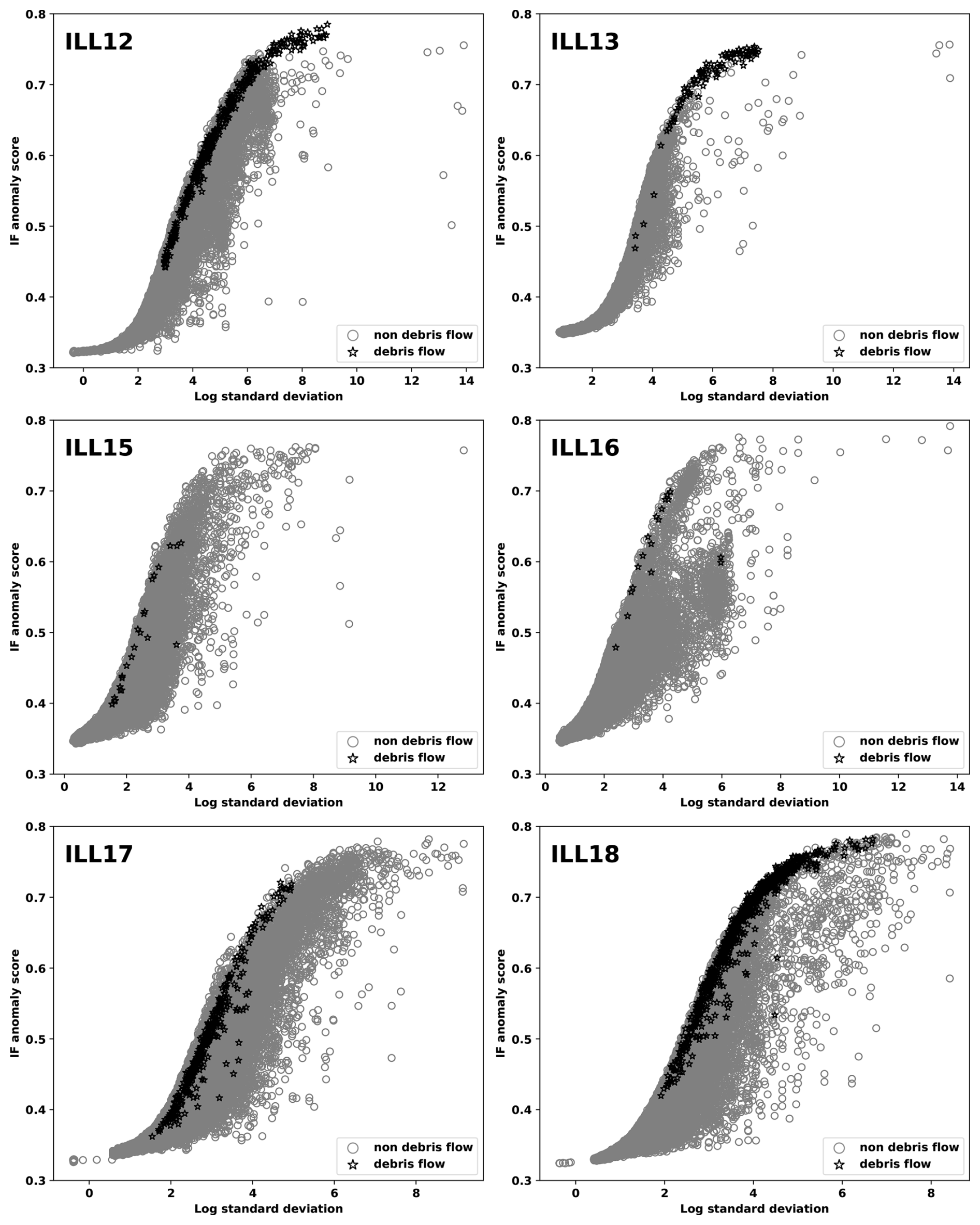
Figure A1 Scatter plots of IF anomaly score against the log standard deviation of time windows observed at stations ILL12, ILL13, ILL15, ILL16, ILL17 and ILL18 during 2018.

A2 Dendrograms

Figure A2 shows complete linkage dendrograms for each station corresponding to the segment DTW distances between high-confidence segments in the WSL catalog over the training period. Singleton merges are defined as those segments that do not merge with a sub cluster and are indicated by bolded lines. These segments are removed before the mean DTW segment distances of IF trigger segments are computed.

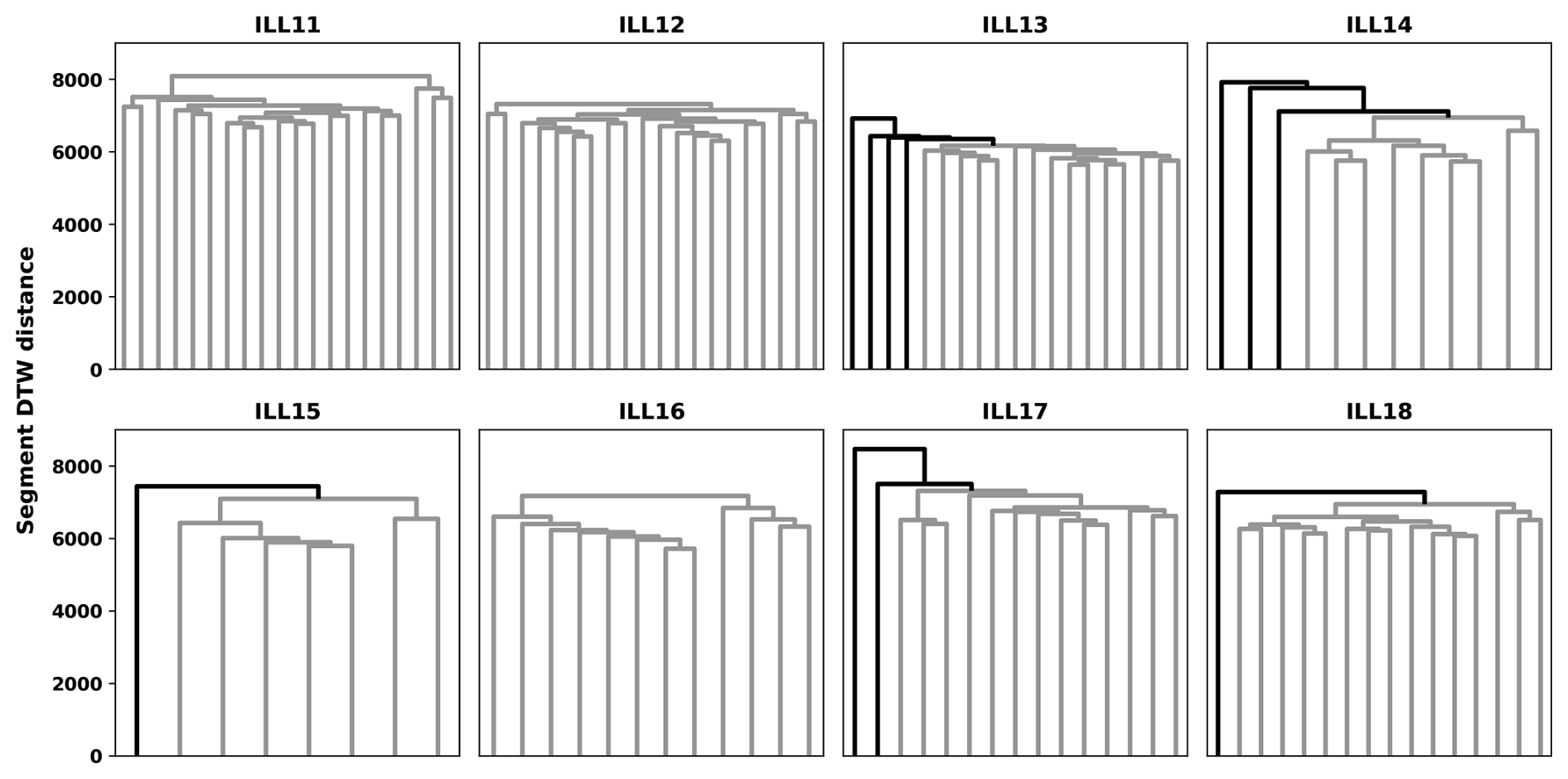
Figure A2 Dendrograms constructed for high-confidence training segments in the WSL catalog for each station in the Illgraben seismic network.

A3 Summary statistics

We give the following summary statistics for the Illgraben seismic network:

• Table A1 contains statistics related to sample sizes.

• Table A2 contains counts of the number of event segments of different confidence levels for each station and year pair, in the WSL and final evaluation catalog.

Table A1 Number of mini-seed recordings (top of each cell) and counts (bottom of each cell) for each station by year in the Illgraben seismic network, before any preprocessing is performed.

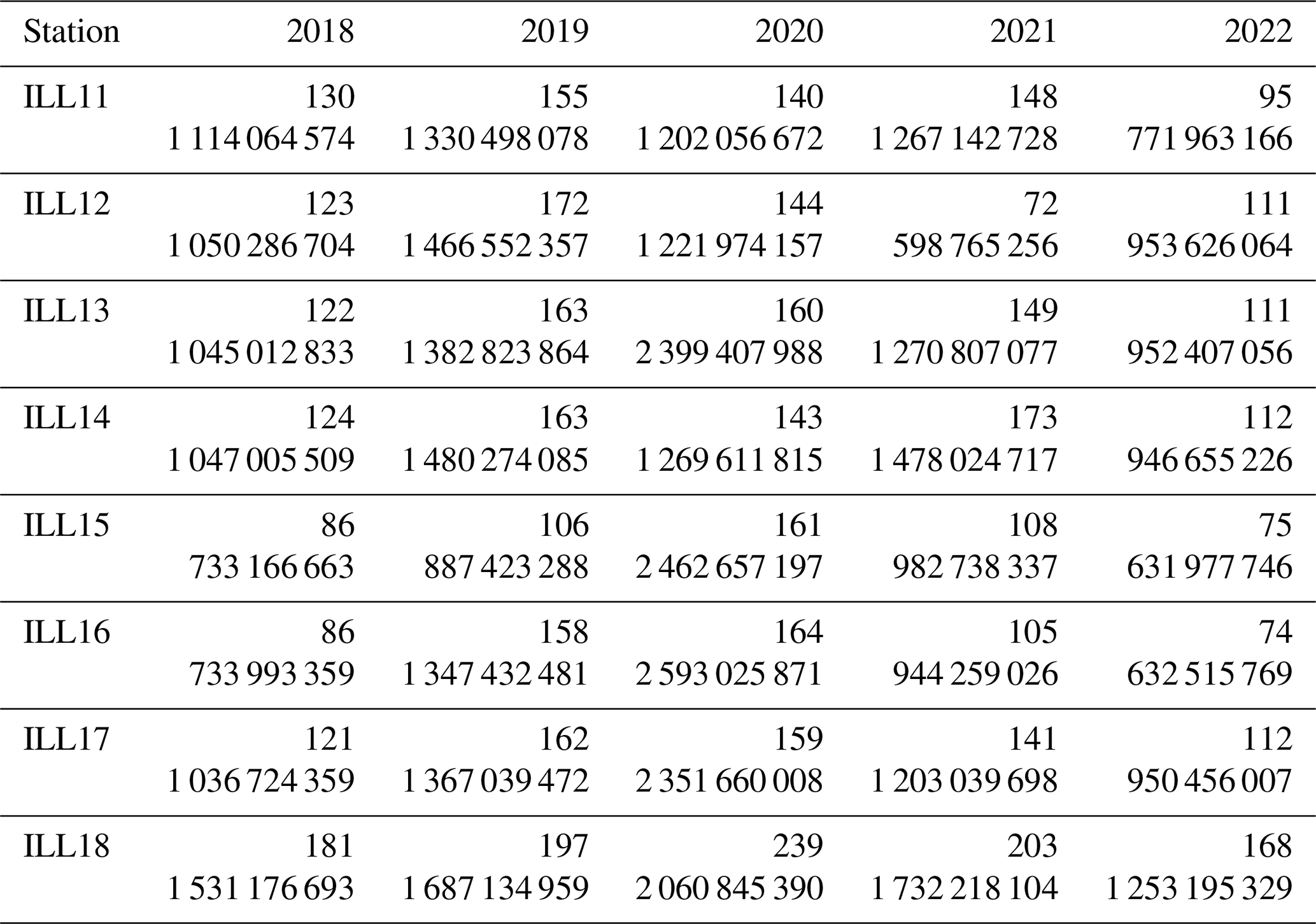
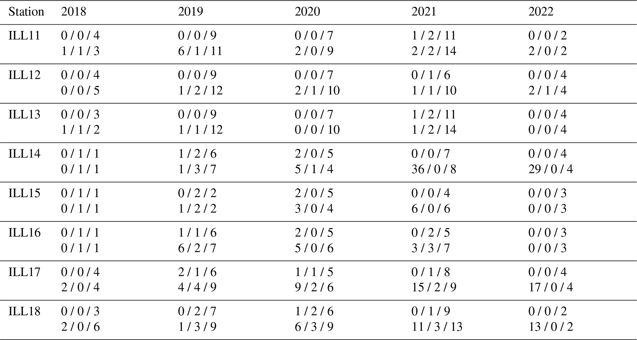
Table A2 Counts of the number of event segments in the initial (above in each cell) and final evaluation (below in each cell) catalogs subdivided by station and year. An entry of $a/b/c$ refers to the number of counts of events of low-, medium- and high confidence.

A4 Hyper parameters

Table A3 contains the chosen hyper parameters for the IF and STA-LTA trigger while Table A4 contain the calibrated thresholds for IF, IF-DTW and STA-LTA workflows.

Table A3 Hyper parameters selected for the IF- and classical STA-LTA trigger. Window sizes are given in seconds.

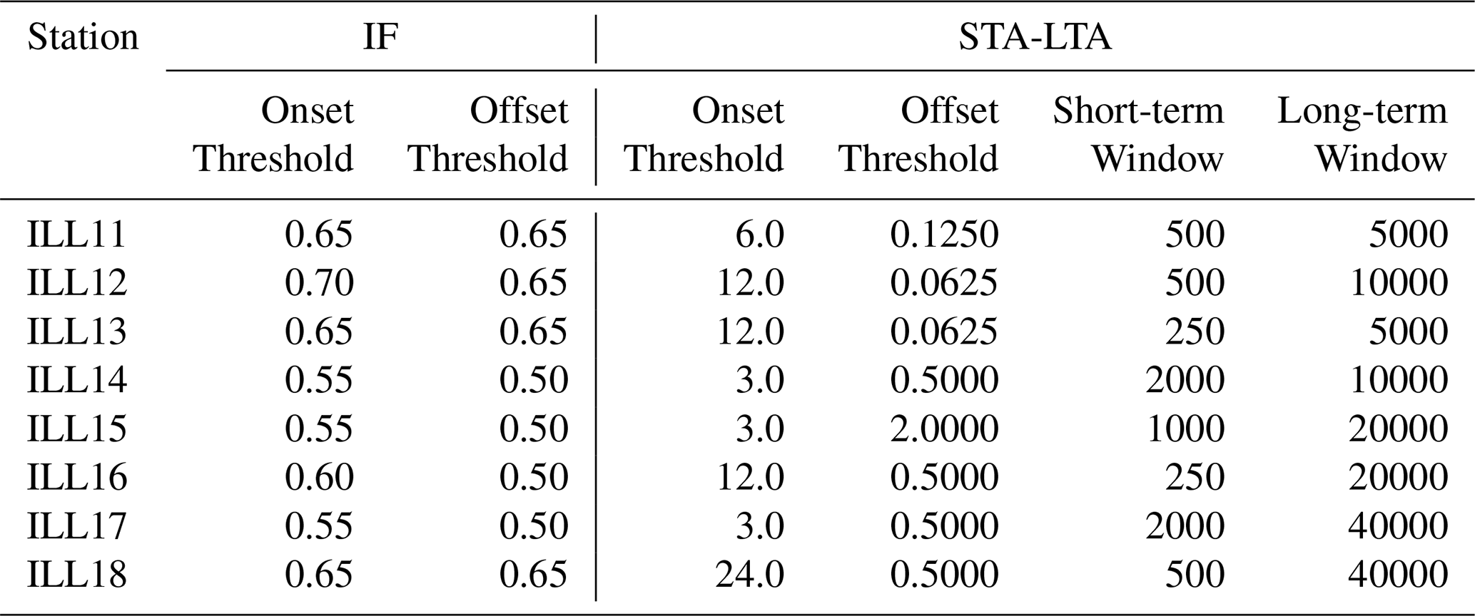
Table A4 Score thresholds and minimum detection lengths calibrated for the IF, IF-DTW and STA-LTA semi-supervised workflows. The score thresholds are given accurate to 4 decimals and minimum detection lengths are given in seconds.

A5 Preprint catalog

The preprint catalog was generated by three major updates of the WSL catalog using the methodology of Fig. 6, and a few smaller updates due to, for example, small experiments. As in the update described in Sect. 3.1.4 the detections made by the IF and STA-LTA workflows at stations ILL14, ILL15, ILL16 and ILL17 were not considered in these updates. Detections at station ILL15 from the IF-DTW workflow was excluded as well because we could not obtain meaningful results here in the preprint. Following two rounds of updates we notice that the upper stations frequently flag segments related to catchment activity as being similar to debris-flows. Such activity includes events such as rockfalls, landslides, and slope failures. Since we are exploring the data, and because this type of activity could related to debris flows, these detections were included as low-confidence debris flow segments in the catalog. After making these changes, one more update of the catalog was performed.

A6 Metrics

Tables A5 and A6 contain comprehensive metrics for each station in the Illgraben network over the training and testing periods, respectively. Tables A7 and A8 show the recall achieved by the IF, IF-DTW and STA-LTA workflows of the lower-confidence catalog segments over the training and test period, respectively. There are more lower- than medium-confidence debris flow segments partly due to the inclusion of catchment and other activity in the lower-confidence class. Overall, the IF-DTW workflow exhibit the highest recall, followed by IF and then STA-LTA.

A7 STA-LTA examples

STA-LTA triggers are known to be sensitive to changes in the amplitude of seismic waveforms. To better capture debris flows, the STA-LTA trigger accommodates for this by taking exceedingly long window lengths, sometimes spanning hours (see Table A3). We illustrate this in Fig. A3, where we study the behavior of the STA-LTA trigger in relation to the seismic waveform observed at ILL11 on 12 June 2018, which contains a debris flow. In all plots, the debris flow is represented by the shaded region. The top graph shows the preprocessed waveform, and the second graph shows the characteristic function of the STA-LTA trigger with the short- and long-term windows given in Table A3. In the remaining plots the window sizes of the STA-LTA trigger are successively divided by two as we proceed towards the bottom. As the window sizes become smaller, it becomes harder to see where the debris flow manifests in the characteristic function.

Having longer window sizes is not without consequence. One particular issue arises when there is increased amplitude (for whatever reason) in the seismic waveform within the long-term or short-term window before a debris flow occurs. Here, the averaging suppresses the characteristic function over the debris-flow period relative to the case if the increase in amplitude did not occur. Managing the trade-off between this phenomenon and the sensitivity towards amplitude can be difficult, particularly in more active stations. We give three examples in Figs. A4, A5 and 9 where two debris-flows occur relatively close in time. The characteristic function over the period associated with the second debris flow is suppressed by the increased amplitude in the seismic waveform over the period associated with the first, leading to false negatives. The IF anomaly score does not suffer from this issue.

Table A5 Metrics over the training period based on the final evaluation catalog. The numbers in brackets in the recall and precision columns represent the number of false negatives and false positives, respectively. All percentages are displayed accurately up to two decimals.

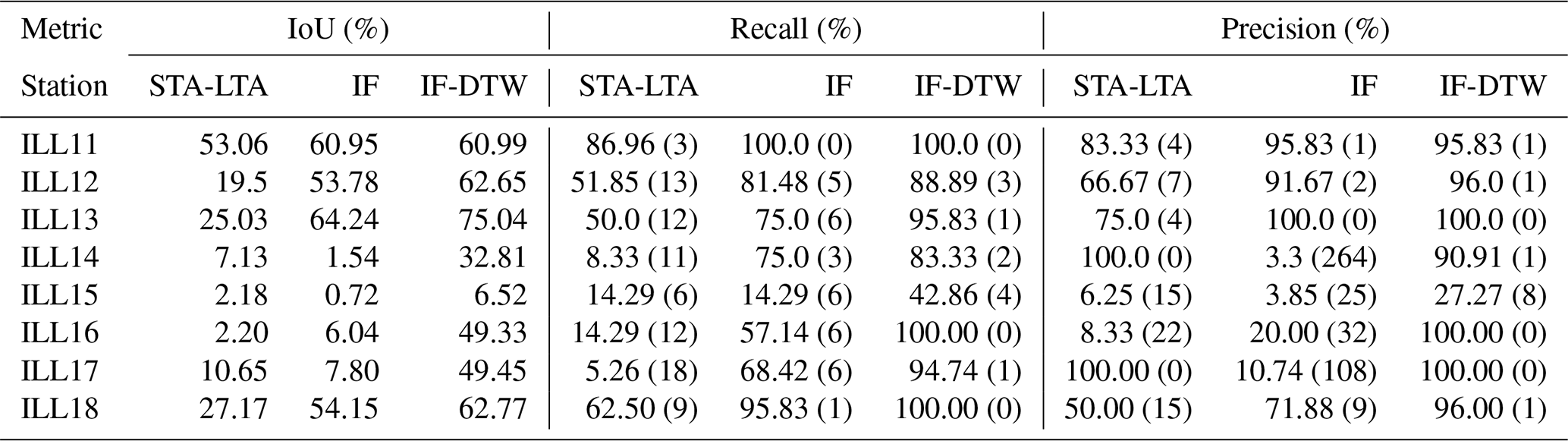
Table A6 Metrics over the testing period based on the final evaluation catalog. The numbers in brackets in the recall and precision columns represent the number of false negatives and false positives, respectively. All percentages are displayed accurately up to two decimals. The symbol “–” means that the corresponding metric could not be computed because no detections were made over the testing period.

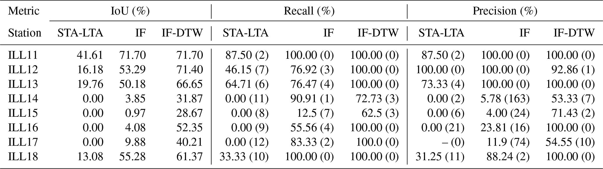
Table A7 Number of events for each confidence class and recall of lower-confidence segments for the different semi-supervised workflows over the training period according to the final evaluation catalog. All values displayed are accurate up to two decimals.

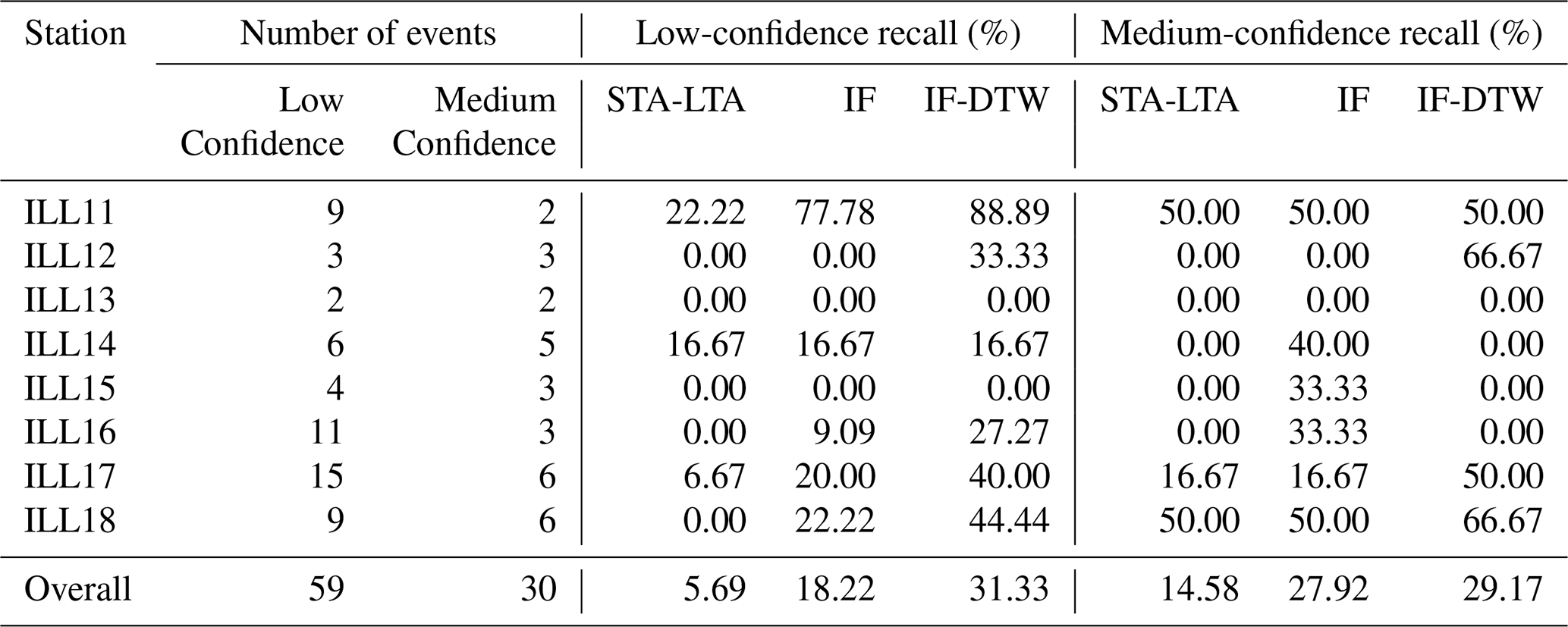
Table A8 Number of events for each confidence class and recall of lower-confidence segments for the different semi-supervised workflows over the testing period according to the final evaluation catalog. All values displayed are accurate up to two decimals.

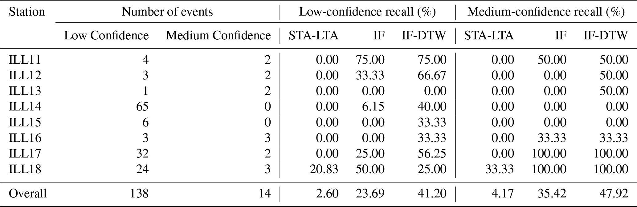
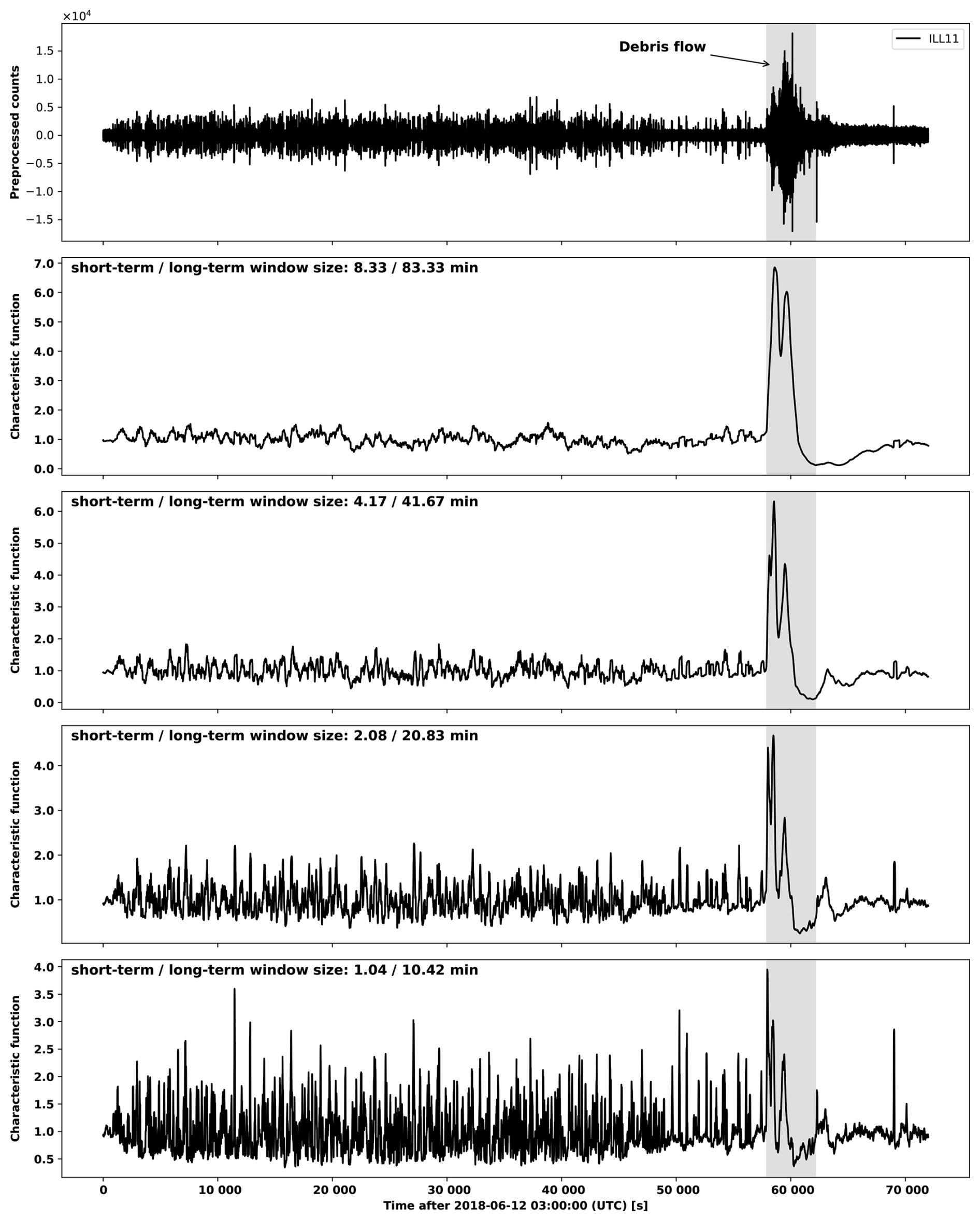
Figure A3 Illustration of the effect of the window sizes on the characteristic function of the STA-LTA trigger.

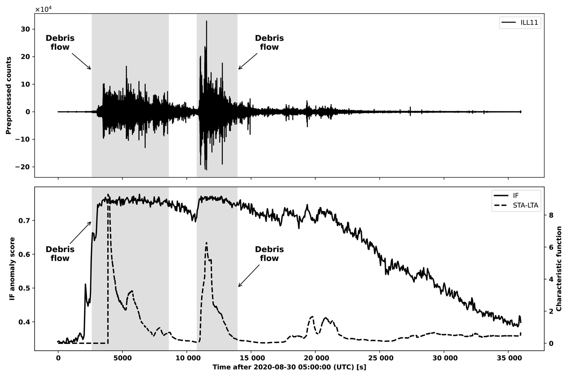
Figure A4 Illustration of the behavior of the STA-LTA characteristic function relative to the IF anomaly score at ILL11 on 30 August 2020. Debris flows are represented by the shaded regions.

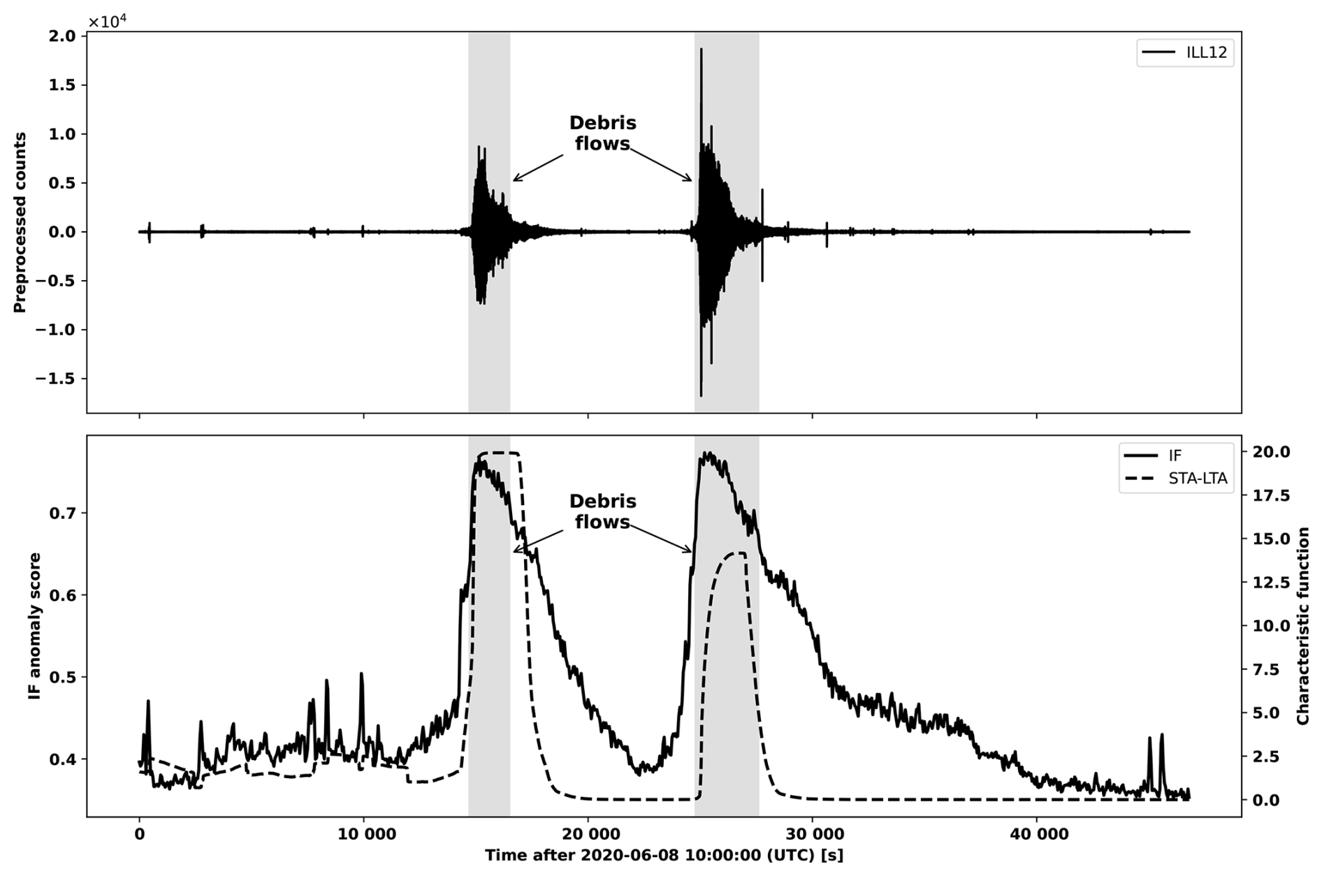
Figure A5 Illustration of the behavior of the STA-LTA characteristic function relative to the IF anomaly score at ILL12 on 8 June 2020. Debris flows are represented by the shaded regions.

Appendix B: Greenland supplementary information

We include the following supplementary information for the case study of Sect. 3.2:

1. Table B1 shows the number of mini-seed recordings and counts for NUUG, KARAT and ILULI.

2. Table B2 shows the leading 10 IF segments among those that are related to mass movements.

3. Figure B1 shows the Ward-linkage dendrogram of the IF segments extracted from the KARAT station.

4. Figure B2 plots the cumulative fraction of mass-movements contained among the leading k IF segments for $k\in \mathit{\{}\mathrm{1},\mathrm{2},\mathrm{\dots },\mathrm{605}\mathit{\}}$.

5. Figure B3 contain time series plots of the amplitude of seismic waveforms and the IF anomaly score for the KARAT station.

Table B1 Number of mini-seed recordings and counts contained in the data used for the case study of Sect. 3.2, before any preprocessing is performed. The relevant years over which the statistics are extracted are contained in the Station column following the colon.

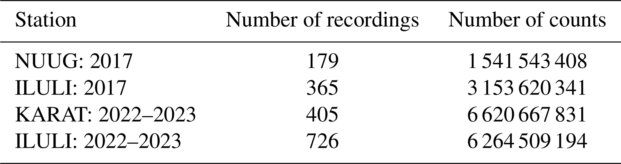
Table B2 Top ranking mass movements detected at KARAT, Greenland. Shown are the starting times of the most anomalous time window according to the IF for each event and the corresponding IF anomaly score. CAL and ID stands for calving and iceberg disintegration events.

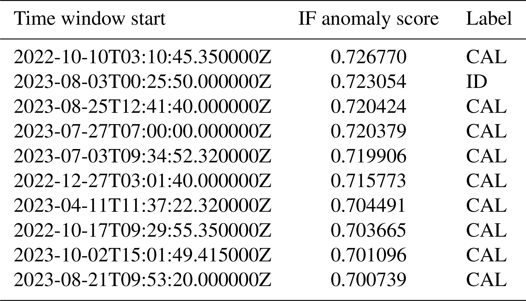
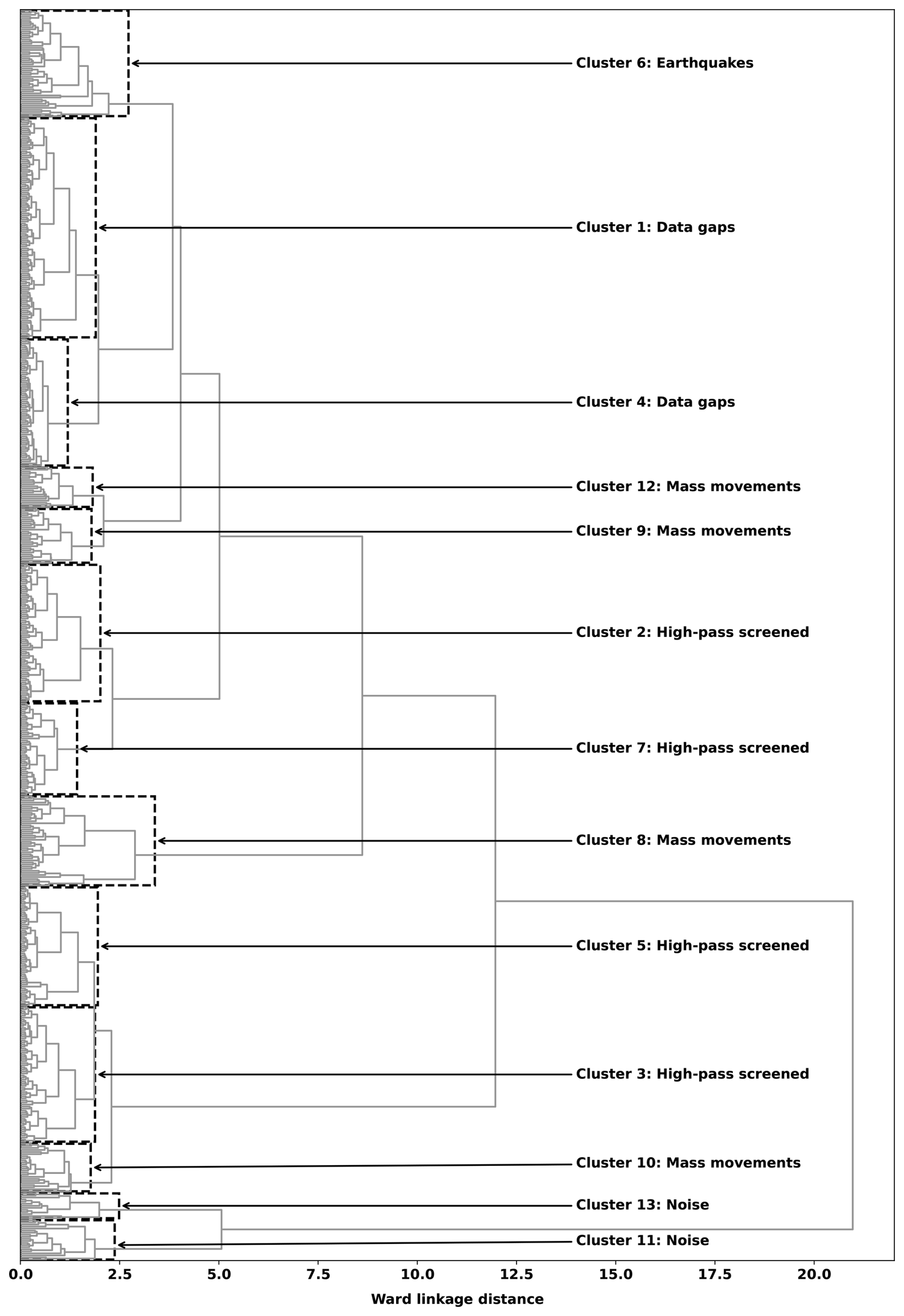
Figure B1 Ward linkage dendrogram of the 605 IF segments flagged at KARAT. Clusters are indicated by bounding boxes. High-pass screened means that after applying the high-pass screening rule described in Sect. 3.2.2 none of the remaining IF segments could be related to mass movements and was not explored further.

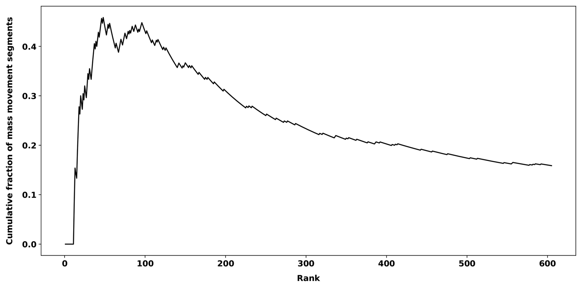
Figure B2 Cumulative fraction of mass-movements contained in the leading $k\in \mathit{\{}\mathrm{1},\mathrm{2},\mathrm{\dots },\mathrm{605}\mathit{\}}$ IF segments according to the IF anomaly score. The index k is represented by the rank label on the x axis.

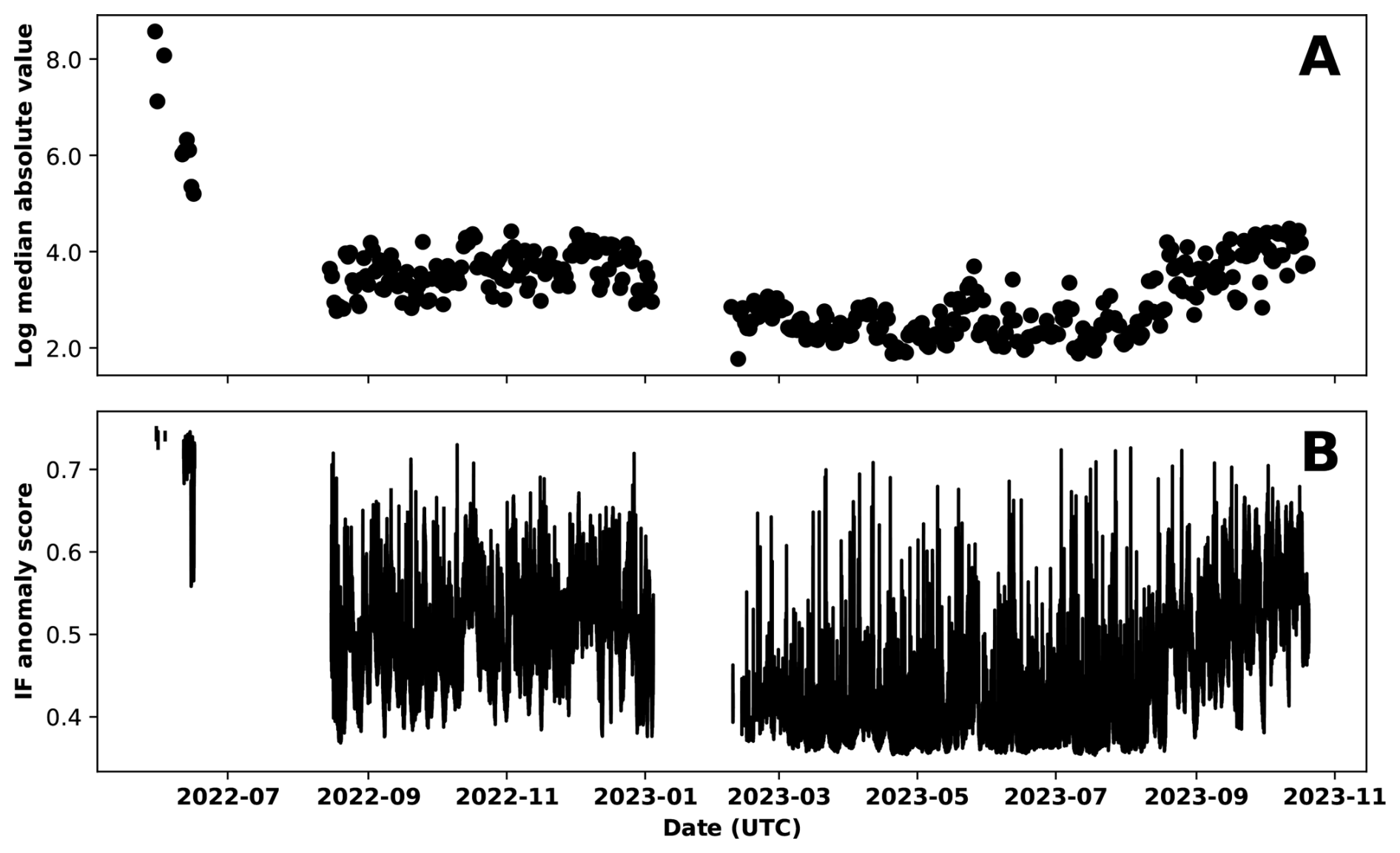
Figure B3 Log median absolute value of the daily preprocessed waveforms (A) and IF anomaly score (B) observed at KARAT.