Buried and displaced: moving characteristics of building fragments in debris flows

Buildings can be destroyed and displaced from their original position in large-scale debris flows and flow-type landslides. Accurate prediction of the relocated position of buildings within debris-flow deposits is urgently needed for emergency rescue. This has been proven to be challenging due to the intricate nature of physical processes. In this study, an elucidation of the complicated physical mechanisms associated with the movement of building fragments within debris flows is provided. Well-controlled flume experiments are conducted and an inertial measurement unit is embedded within the model of the building block to monitor the block's movement mode. An analytical model considering the hydrodynamic drag force, earth pressure, and basal friction is further established. Dimensionless parameters are derived to clarify the underlying physical mechanisms. The results demonstrate that the deposition position of building fragments is predominantly governed by the basal sliding velocity of debris flow. The dimensionless parameter αFr² informs optimal model selection to enhance predictive accuracy within this framework. These findings provide useful reference for post-disaster emergency rescue by enabling precise positioning of buried structures.

1 Introduction

Debris flow is a hydrological phenomenon that possesses immense destructive power. The core characteristic of a debris flow is its low effective stress, corresponding to a high degree of liquefaction (Iverson et al., 2015). The damage inflicted upon buildings by debris flows comes in several forms: dynamic impact, static inundation, and abrasion (Wang et al., 2023; Zeng et al., 2014; Zhao et al., 2025). The most significant hazard posed by large-scale debris flows is the burial and displacement of damaged buildings and the victims trapped inside. Buildings are displaced from their original locations (Luo et al., 2019), making emergency rescue considerably challenging.

A typical example is exhibited in the 2010 Zhouqu debris flow (Hu et al., 2012). A debris flow with a height of several meters caused “collapse like dominoes”, completely destroying 33 buildings, causing death of 1557 individuals, with 284 reported missing. Similarly, the landslide-debris flow in Guangming, Shenzhen, China (Fig. 1), had a maximum mobility of 1120 m and a deposition thickness of 8–20 m. It destroyed and buried 33 buildings, with 77 victims missing. Post-event field surveys revealed that the horizontal displacement of the building could reach up to 150 m (Luo et al., 2019), which poses significant challenges for rescuers to locate victims trapped in displaced buildings. In 2019, the landslide-debris flow in Shuicheng, Guizhou, China (Zhao et al., 2020) travelled over 1250 m, with 21 buildings damaged or buried and 9 victims missing. Due to the steep terrain, some buildings were displaced as far as 400–500 m downstream. In the 2014 Oso landslide in the United States, the travel distance exceeded 1 km, resulting in 43 deaths or missing persons. Survivors were displaced approximately 210 m in a wooden house, with a lower density than that of the flow (Wartman et al., 2016). Given these characteristics, it was recommended that rescuers search for trapped individuals at the front of the deposition, rather than at the original location of the buildings.

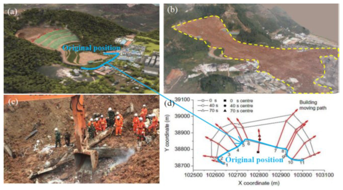
Figure 1 A typical case of landslide-debris flow at Guangming, Shenzhen, China (Yin et al., 2016). (a) Landform before landslide; (b) buried area after landslide; (c) state of buried building fragment (https://www.chinadaily.com.cn/, last access: 20 December 2015); and (d) moving direction and displacement of buildings (Luo et al., 2019).

The highly destructive power of debris flows is attributed to their high mobility and loads. Recent studies have emphasized the importance of solid-liquid coupling (Iverson, 2015) in regulating debris-flow mobility and dynamic loads (Song et al., 2023). By considering the particle dilation and pore-water pressure at the microscopic level, Iverson and George (2014) studied the physical mechanism behind the high mobility of Oso landslide. It is confirmed that an increase in pore-water pressure caused by particle shearing in loose soil (an increase in overall degree of liquefaction) is the primary factor controlling debris-flow mobility and its ability to displace and bury buildings. Through field investigation and numerical analysis, Collins and Reid (2020) revealed that local liquefaction in the contact area with the bed caused the high mobility of Oso landslide. The debris and buildings displaced above the liquefied layer displayed characteristics of integral movement (Zhang et al., 2021), contributing to the preservation of building integrity. The regulation of solid-liquid coupling in debris flows also plays a crucial role in the interaction between the debris flow and structures such as buildings. When a high-concentration debris flow, where friction plays a dominant role, comes into contact with a structure, the generated local shear quickly dissipates the kinetic energy (Song et al., 2019) and transforms into static deposition (Song et al., 2017). Therefore, the force acting on the building is a combination of the dynamic load of the flow and the static load of the deposition. For both dry granular (Faug, 2015) and two-phase granular-fluid flows (Sturm et al., 2018), this force can be expressed as a function of the Froude number of the incoming flow.

Currently, a few studies have focused on the movement of individual boulders in debris flows, which provide a valuable reference for the study of building fragments movement in debris flows. Ng et al. (2021) derived a theoretical model of a single boulder under the drag force of a debris flow and verified the theoretical prediction through large-scale flume experiments. However, the theoretical model does not consider the interaction between the block and bed, i.e., the basal friction. In coastal engineering, the movement of individual blocks by tsunamis has been well studied, and the proposed theoretical models for boulder movement under tsunami traction also provide useful reference for the study of building fragment movement. It is revealed that the shape (Goto et al., 2007; Harry et al., 2019; Oetjen et al., 2020), density, quantity (Nandasena and Tanaka, 2013), flow direction (Iwai and Goto, 2021), and block orientation (Goto et al., 2007; Liu et al., 2014; Nandasena and Tanaka, 2013) all affect its mode of movement and deposition. Moreover, the opacity of debris flows increases the difficulty of studying the movement of internal blocks. By placing inertial measurement units (IMUs) within a block, researchers and engineers can gather real-time information about the block's behavior and response to debris flows, which helps in understanding the dynamics of block motion (Caviezel et al., 2021; Maniatis, 2021). Based on USGS large-scale debris-flow flume experiments, Harding et al. (2014) integrated an inertial measurement unit (IMU) into a sealed block to track its trajectory within a debris flow by recording the acceleration and angular velocity, but the calculation of position is subject to significant errors due to the orientation bias of the IMU gyros.

Currently, there is a critical gap in the fundamental understanding of the physical mechanisms governing interactions between debris flows and structural fragments. This knowledge deficit significantly hampers the accurate localization of trapped victims and compromises the effectiveness of emergency rescue operations. In this study, well-controlled experiments are carried out to reveal the physical processes of building fragments movement within debris flows. An analytical model is further proposed to predict the location of building fragments within debris-flow deposition. The model performance is verified against the experimental results. The primary objective of this study is to elucidate the key factors governing the displacement of building fragments by debris flows. By achieving this goal, the study aims to provide valuable reference for emergency rescue.

2 Model experiments and physical processes revealed

Scaled laboratory experiments serve as a prevalent methodology in research of debris flow dynamics, which allow researchers to exert precise control over experimental parameters and facilitate systematic measurement. Consequently, the obtained results facilitate to reveals the physical processes of debris flow-building fragments interaction and provide robust validation for theoretical models' predictions.

2.1 Experimental model setup

A bilinear flume is adopted to model the block movement under the action of debris flow (Fig. 2a). The upstream section is 4 m long and inclined at 25°. The top 1 m acts as a reservoir that is isolated by an uplift gate for releasing debris material. The downstream section has a length of 6 m and is inclined at 5° which is a typical slope for the deposition area. The width of the flume is 0.3 m, and the sidewall is transparent for observing the movement of the block. Spherical glass beads (0.6 mm) are used to roughen the flume bed, which is also used as the solid phase of debris flow. A flat aluminium block is positioned 0.75 m downstream from the smooth transition zone (Fig. 2a).To ensure that the block only moves by sliding rather than rolling and saltation, the block is designed as a flat shape, and the edges are rounded. The dimension of the block is 40 mm × 40 mm × 10 mm (Fig. 2b). The debris flow accelerated after being released upstream and began to decelerate (deposit) after reaching the 5° section.

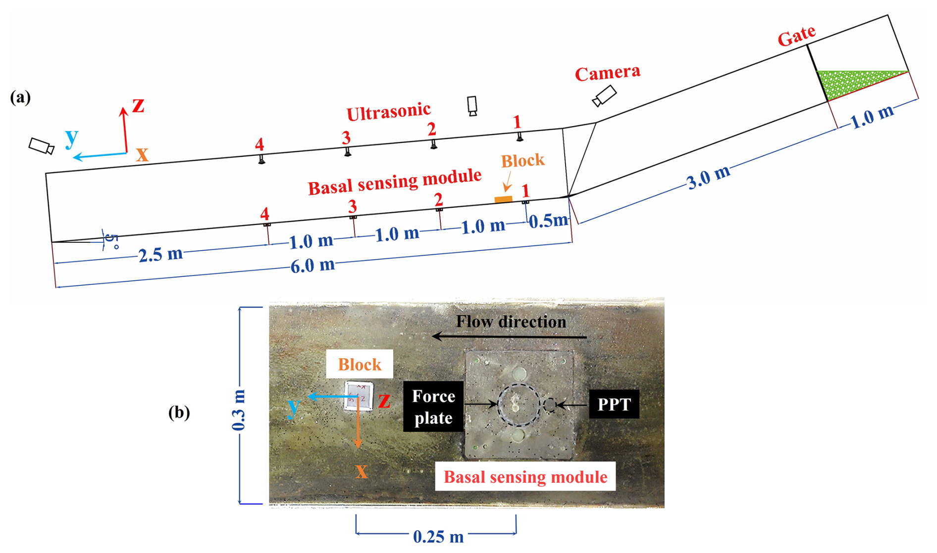
Figure 2 Experimental setup and instrumentation: (a) flume set-up; (b) basal sensing module for measurement of normal/shear stresses and pore-water pressure, and a 40 mm × 40 mm × 10 mm block with inertial measurement unit (IMU).

2.2 Instrumentation and materials

The flume bed contains 4 basal sensing modules (Fig. 2a), and each module is equipped with a triaxial load cell (LH-SZ-02, 50N, ±0.1 % BSL) located at the center of the force plate (Fig. 2b). These load cells are used to measure normal and shear stresses. Additionally, each module has a pore-water pressure transducer (PPT, OMEGA PX409, 6.9 kPa/34.5 kPa, ±0.08 % BSL) upstream of the force plate (Fig. 2b) to measure pore-water pressure. Above each basal sensing module, there is an ultrasonic sensor (BANNER U-GAGE T30UXUA, 0.1–1.0 m, resolution 0.1 % of distance) to measure the flow depth. The whole data acquisition system (National Instruments) is set to a sampling rate of 500 Hz. To derive the frontal velocity prior to contact, a high-speed camera (PHONTRON FASTCAM Mini WX50) with resolution of 1280 × 1024 pixels is placed at the sidewall of the flume. The frame rate of the high-speed camera is set at 250 fps. Three video cameras (DJI Osmo Action 4, resolution 3648 × 2736 pixels, 120 fps) are used to capture the movement kinematics.

Owing to the incomplete transparency of the modeled debris flow, the block movement is not easily observable by eye. Therefore, employing a micro inertial measurement unit (IMU) is imperative for analyzing its movement mode (Curley et al., 2021; Maniatis, 2021). A commercial IMU (WITMOTION, WT901SDCL) is embedded into the block. It has an acceleration range of ±16 g with accuracy of 0.0005 g per LSB (least significant bit), and an angular velocity range of ±2000° s⁻¹ with resolution of 0.061 (° s⁻¹) per LSB. The sampling rate of the IMU is 200 Hz. The IMU can be switched on and off manually before and after the experiments. Through the images captured by the high-speed camera, the response of IMU can be manually synchronized with the flow depth and stress measurements.

For the basal sensing modules, the raw data from the load cells and the pore-water pressure transducer exhibit substantial noise. To facilitate data visualization and comparison, a moving average filtering (with interval of 0.02 s) is employed to smooth these datasets. The raw data from the IMU are retained without filtering.

In this study, glass beads with diameters of 0.6 mm and densities of 2540 kg m⁻³ are used as the solid phase of debris flows. A solution of glycerol and water is used as the fluid phase. The blocks have a density (2700 kg m⁻³) close to that of reinforced concrete.

2.3 Test program

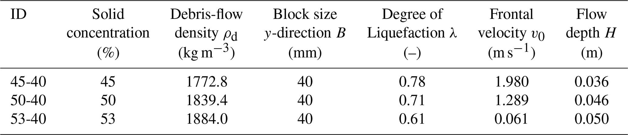
To investigate the mechanism of debris flows displacing building blocks under different flow conditions, debris flows are modeled with volumetric solid concentrations of 45 %, 50 %, and 53 % (Table 1). The fluid viscosity is kept at 0.01 Pa s, i.e., ten times that of water. The solid particles and fluid phase are thoroughly mixed using a mixer before release. The debris-flow volume is 50 L. A steady flow with relatively constant height is generated by adjusting the opening of the gate. The test program of this study is summarized in Table 1.

Table 1 Test program and measured parameters.

2.4 Experimental results

2.4.1 Observed kinetics of blocks displaced by debris flows

Figure 3 illustrates the interaction process of a 50 % concentration debris flow with the block (Test 50-40, Movie S2 in the Supplement). The flow front contacts the block and forms a slight jump (Fig. 3b). Then, the block starts to be displaced and buried by debris (Fig. 3c), and finally stops in the debris-flow deposition (Fig. 3d and e). Throughout the entire process, the flow depth of the debris flow remains constant, and the frontal velocity decreases gradually. The block movement under debris flows with solid concentrations of 45 % and 53 % can be found in Movies S1 and S3.

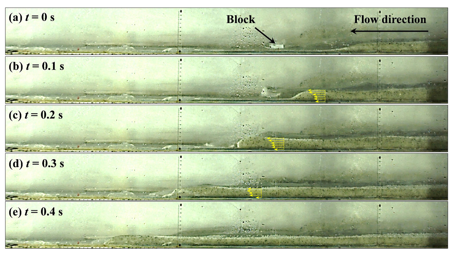
Figure 3 Sequence of side-view images of Test 50-40. (a) The incoming flow with steady flow depth; (b) the flow front contacts the block, (c) the block is buried and displaced by subsequent flow, and (d–e) block stops in the deposition. The velocity profiles are shown by yellow arrows.

Based on high-speed photography, Particle Image Velocimetry (geoPIV8, Take, 2015) analysis is conducted to determine the velocity profile within the debris flow (Fig. 3b–d). The results reveal distinct basal sliding, evidenced by non-zero flow velocities in the near-bed region. The basal slip has also been observed at the Lattenbach catchment, Tyrol, Austria, particularly during surge phases and granular flow fronts (Nagl et al., 2026). The velocity profile exhibits a predominantly linear distribution extending from the free surface to the substrate interface. Quantitative analysis demonstrates that the basal sliding velocity attains approximately 60 % of the frontal flow velocity.

2.4.2 State of debris flow revealed by basal measurement

Figure 4 presents the measured normal stress, shear stress, and pore-water pressure of the modeled debris flows. Figure 4a–c illustrate the data collected from the experiments with a 45 % concentration. Owing to its high mobility (high degree of liquefaction), the debris flow passes through three basal sensing modules (B1, B2, and B3). For the experiment with a 53 % concentration, which has low mobility (low degree of liquefaction), only basal sensing module B1 is covered by debris flow (Fig. 4f). For the experiment with a 50 % concentration, which has intermediate mobility, basal sensing modules B1 and B2 are covered by debris flow (Fig. 4d-e). The passage of debris flow is reflected by the sharp increase in stress and pore-water pressure, and the debris-flow average velocity between two basal sensing modules is calculated based on the difference of response time.

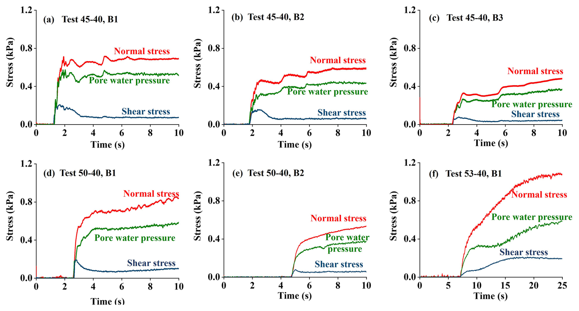
Figure 4 Measured basal normal stress, shear stress, and pore-water pressure. (a–c) Test 45-40 at basal sensing module B1and B2, and B3; (d–e) Test 50-40 at B1 and B2; (f) Test 53-40 at B1.

Solid concentration is the key factor controlling the flow state of debris flows. The 45 %-concentration debris flow is more mobile than the 50 %- and 53 %-concentration flows. Furthermore, the degree of liquefaction of debris flow is positively correlated with the solid concentration. Specifically, the lower the solid concentration, the higher the degree of liquefaction and the weaker the effective stress (e.g., 0.78 for 45 %-concentration vs. 0.61 for 53 %-concentration in Table 2), resulting in a higher mobility of the debris flow (Collins and Reid, 2020). Modeled debris flows with low concentrations have higher flow velocities and shallower flow depths compared to those with high concentrations (Movies S1, S2, and S3).

Table 2 Test results and dimensionless parameters.

A low concentration leads to a high Fr with a high flow velocity and low flow depth, resulting in a rapid increase in the stress response (Fig. 4a) and quickly reaching a stable value. In contrast, debris flows with a high solid concentration have low Fr values, low flow velocities, high flow depths, and gradual increases in stress (Fig. 4f). The rapid increase in stress and pore pressure affects the acceleration of the block upon contact with the debris flow. The trend of stress and pore pressure rises faster, and the block experiences a greater acceleration at the moment of contact (further see Fig. 6). This poses risks to building integrity and victim safety.

2.4.3 Block position within debris-flow deposition

To determine the depositional position of blocks within debris-flow deposits and facilitate comparative analysis of experimental results, the relative block position is quantified as the ratio of block displacement distance (L) to debris-flow deposit length (S) as $L/S$. This dimensionless parameter, summarized in Table 2, is subsequently adopted as the predictive output in our theoretical framework.

The debris-flow deposition profile and block position are illustrated in Fig. 5. The deposition depth is measured at intervals of 0.5 m along the transparent sidewall, and the block position is determined by manual search. Clearly, the high degree of liquefaction of low-concentration debris flows results in less resistance and thus the greatest runout distance. As the concentration increases, the debris-flow runout distance decreases, and the block travel distance shortens accordingly (Fig. 5). However, experiments with 53 %-concentration debris flows have the highest $L/S$, followed by 50 % and 45 % (Fig. 5). The block position is closer to the deposition front, because earth pressure dominates in high-concentration debris flows.

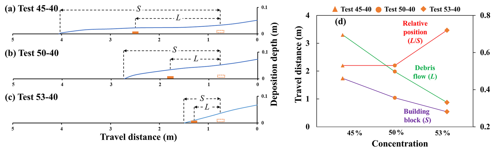
Figure 5 The debris-flow deposition profile and block position in the deposition. (a) Test 45-40; (b) Test 50-40; (c) Test 53-40; and (d) comparison of travel distance and relative position.

2.4.4 The block posture revealed by the inertial measurement unit

The flow depths of debris flows are greater than the block height, resulting in complete submersion of the block. The triaxial acceleration of the block with embedded IMU are shown in Fig. 6. The x, y, and z axes represent pitch, roll, and heading angles, respectively.

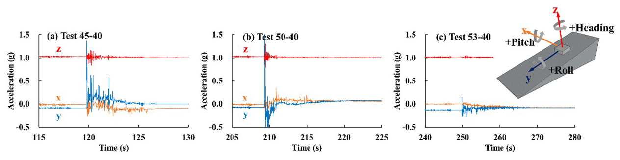
Figure 6 Measured triaxial acceleration of (a) Test 45-40, (b) Test 50-40, and (c) Test 53-40. When the block is at rest, the z axis has an acceleration of nearly 1 g and the acceleration of the y axis of the block is not zero due to the 5° slope of flume.

We adopt the measured acceleration to infer the real-time state of the displaced block. At the moment of contact, the y-axis acceleration increases sharply, resulting in downward block movement. Meanwhile, the z axis maintains a constant upward acceleration of 1 g throughout the entire process, indicating that the direction of the z axis does not change during the whole process. That is, the block does not roll over (y direction). For Test 45-40, after debris-flow deposition, the accelerations of the x and y axes are swapped (Fig. 6a), indicating that the block rotated 90° around the z axis. For Test 50-40, the x and y axes exhibit similar accelerations after deposition (Fig. 6b), indicating that the block rotated 45° around the z axis from its original position.

Debris flows with low concentration and high mobility lead to sharp increase in acceleration during the initial contact with the block. The fluctuations reflect the duration of the entire interaction process, including the initial contact of the debris flow on the block and the subsequent slow movement of the deposition. For instance, in debris flow with 53 % concentration, the acceleration and angular velocity fluctuations persist for 20 s. In contrast, the debris flow with 45 % solid concentration only lasts 5 s before the block comes to stop.

Based on the data from the IMU, the block exhibits impulsive acceleration characteristics during the initial contact. This indicates that the block gains high initial velocity through contact with the flow front. By integrating the y axis acceleration within the initial 0.2 s, the initial velocity of the block can be obtained. We determine the dimensionless initial velocity m (block initial velocity over the velocity of debris flow) of the block as m = 0.9 for experiments with 45 % and 50 % solid concentration and m = 1.0 for 53 % solid-phase concentration. These dimensionless initial velocities serve as input for the model prediction in the next section.

3 Development of the analytical model

In this section, we first introduce the well-known leading-edge model (Takahashi and Yoshida, 1979), and then derive the governing equations for fragment movement based on this model. Nondimensionalization of governing equations results in the identification of several new dimensionless numbers. Next, we classify the models and their solutions according to the magnitude of these dimensionless numbers.

3.1 The leading-edge model

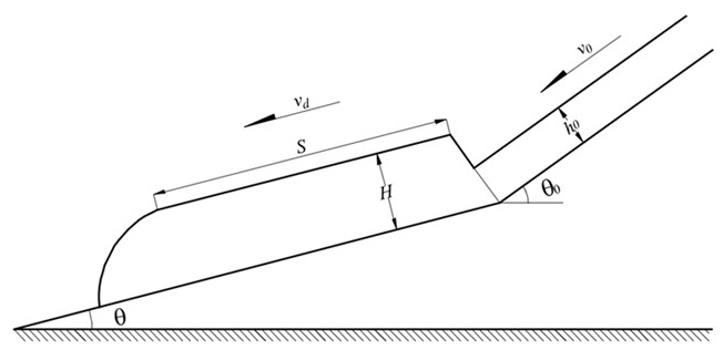
The leading-edge model developed by Takahashi and Yoshida (1979) is introduced. When the debris flow (with velocity v₀ and depth h₀) enters into deposition area (slope θ), the velocity v_d slows down, and the flow depth H thickens. The debris-flow deposition is regarded as a cohesive whole. Compared with the original model, we further consider the influence of the degree of liquefaction on basal friction resistance.

Figure 7 Schematic diagram of leading-edge model.

According to the conservation of mass and momentum in the flow area and accumulation zone, the governing equations (conservation of mass and momentum) are expressed:

$$\begin{array}{}\text{(1)}& {\displaystyle }HS=h_{\mathrm{0}}{v}_{\mathrm{0}}t\text{(2)}& {\displaystyle }\begin{array}{l}\frac{\mathrm{d}}{\mathrm{d}t}\left({\mathit{\rho }}_{\mathrm{d}}HvS\right)={\mathit{\rho }}_{\mathrm{d}}gHS\sin \mathit{\theta }\mathrm{\text{Gravitational driving force}}\\ -{\mathit{\rho }}_{\mathrm{d}}gHS\cos \mathit{\theta }\left(\mathrm{1}-\mathit{\lambda }\right){\mathit{\mu }}_{\mathrm{d}}\mathrm{\text{Frictional resistance}}\\ +\left({\mathit{\rho }}_{\mathrm{d}}{h}_{\mathrm{0}}{v}_{\mathrm{0}}\right)v_{\mathrm{0}}\cos \left({\mathit{\theta }}_{\mathrm{0}}-\mathit{\theta }\right)\mathrm{\text{Momentum flux of upstream}}\\ +{\displaystyle \frac{\mathrm{1}}{\mathrm{2}}}k{\mathit{\rho }}_{\mathrm{d}}g{h}_{\mathrm{0}}^{\mathrm{2}}\cos {\mathit{\theta }}_{\mathrm{0}}\cos \left({\mathit{\theta }}_{\mathrm{0}}-\mathit{\theta }\right)\mathrm{\text{Earth pressure of upstream}}\end{array}\end{array}$$

where ρ_dHvS is the momentum of deposition, and its time derivative is the force on the deposition. On the right-hand side of Eq. (2), all the forces acting upon the deposition are summed up. The first row is gravitational driving force, and the component of the gravity of deposition along the flow direction; the second row is the frictional force generated by self-weight considering the degree of liquefaction λ and friction coefficient between flow and bed μ_d; the third row is the momentum flux of the incoming flow, where v₀, h₀, and θ₀ are velocity, depth, and slope of upstream; the last row is the earth pressure from the upstream to the downstream, and k is the earth pressure coefficient. Substitute Eq. (1) into Eq. (2):

$$\begin{array}{}\text{(3)}& \begin{array}{l}\frac{\mathrm{d}}{\mathrm{d}t}\left(v_{\mathrm{d}}t\right)=g\left(\sin \mathit{\theta }-\cos \mathit{\theta }\left(\mathrm{1}-\mathit{\lambda }\right){\mathit{\mu }}_{\mathrm{d}}\right)t\\ +v_{\mathrm{0}}\cos \left({\mathit{\theta }}_{\mathrm{0}}-\mathit{\theta }\right)\left(\mathrm{1}+\frac{k}{\mathrm{2}{\mathit{Fr}}_{\mathrm{0}}^{\mathrm{2}}}\right)\\ =-G_{\mathrm{d}}t+v_{\mathrm{1}}\end{array}\end{array}$$

where G_d = $g\left({\mathit{\mu }}_{\mathrm{d}}\cos \mathit{\theta }(\mathrm{1}-\mathit{\lambda })-\sin \mathit{\theta }\right)$ is the acceleration of the deposition downslope, v₁ = $v_{\mathrm{0}}\cos \left({\mathit{\theta }}_{\mathrm{0}}-\mathit{\theta }\right)\left(\mathrm{1}+\frac{k}{\mathrm{2}{\mathit{Fr}}_{\mathrm{0}}^{\mathrm{2}}}\right)$ is the equivalent upstream inflow velocity, Fr₀ = $\frac{v_{\mathrm{0}}}{\sqrt{g{h}_{\mathrm{0}}\cos {\mathit{\theta }}_{\mathrm{0}}}}$ is the Froude number of upstream incoming flow. We further solve Eq. (3) and obtain the velocity of debris flow:

$$\begin{array}{}\text{(4)}& \begin{array}{l}{v}_{\mathrm{d}}=-\frac{\mathrm{1}}{\mathrm{2}}g\left(\cos \mathit{\theta }\left(\mathrm{1}-\mathit{\lambda }\right){\mathit{\mu }}_{\mathrm{d}}-\sin \mathit{\theta }\right)t\\ +v_{\mathrm{0}}\cos \left({\mathit{\theta }}_{\mathrm{0}}-\mathit{\theta }\right)\left(\mathrm{1}+\frac{k}{\mathrm{2}{\mathit{Fr}}_{\mathrm{0}}^{\mathrm{2}}}\right)\\ =-\frac{G_{\mathrm{d}}}{\mathrm{2}}t+v_{\mathrm{1}}\end{array}\end{array}$$

From the solution, the debris flow in the deposition area is in uniform deceleration motion, and the deceleration is $\frac{G_{\mathrm{d}}}{\mathrm{2}}$. The equivalent upstream inflow velocity v₁ is not used in the next sections, because the velocity of the debris flow at the downstream can be directly measured in the experiment, and v₀ is used to represent the initial frontal velocity of debris flow at the downstream start. The deposition length of debris flow can be obtained by integrating the velocity:

$$\begin{array}{}\text{(5)}& \begin{array}{l}S=v_{\mathrm{1}}t-\frac{\mathrm{1}}{\mathrm{4}}{G}_{\mathrm{d}}{t}^{\mathrm{2}}\\ =\frac{\mathrm{2}{v}_{\mathrm{1}}^{\mathrm{2}}}{G_{\mathrm{d}}}\end{array}\end{array}$$

3.2 Model of debris flow displacing a building fragment

Based on the aforementioned leading-edge model, we developed a model where the kinematic behavior of building blocks is exclusively governed by the debris flow dynamics, with negligible feedback effects on the flow regime. This hypothesis generally requires the ratio between mass of debris flow (discharge) and the mass of block to be higher than 10.

As a preliminary study focusing on mechanisms, the proposed model in this study only considers the movement of one single building fragment. This means the complicated destruction process of buildings is not covered. Without a deep understanding on the mechanisms of a simplified scenario, it is pessimistic to further forward our understanding into the complicated real-world cases. When the density of building fragment is higher than that of debris flow, the fragment sinks and contacts the bed (Fig. 8). The motion of a fragment sinking to the bed can be influenced by flow conditions and local terrain, leading to various forms of movement, such as sliding, rolling, and saltation (Imamura et al., 2008; Nandasena and Tanaka, 2013). The movement of a fragment can also be affected by factors such as its shape, size, and density, as well as the forces it experiences. Since the fragments of destroyed buildings are mostly flat, we consider that the movement mode of the fragment (block) is sliding.

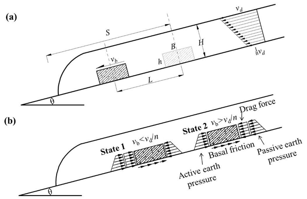
Figure 8 Schematic diagram of (a) block moving along with decelerating debris flow, with velocity profile; (b) forces acting on the block: drag force, basal friction, and active/passive earth pressures.

Based on Takahashi and Yoshida's model, a flat block sinks at the bed under a decelerating incoming flow condition and is displaced a certain distance from its initial position. During the movement, we assume that the forces acting on the block can be described as the sum of its own gravity, buoyancy, friction resistance, dynamic drag force, and active/passive earth pressures (Fig. 8). Compared to the drag force, the fluid viscous force is negligible (with the Friction number; Iverson, 2015; higher than 100), hence it is not considered in the model. The governing equation of block movement can be expressed:

$$\begin{array}{}\text{(6)}& \begin{array}{l}{\mathit{\rho }}_{\mathrm{b}}{V}_{\mathrm{b}}\frac{\mathrm{d}{v}_{\mathrm{b}}}{\mathrm{d}t}=C_{\mathrm{d}}{\mathit{\rho }}_{\mathrm{d}}A{\left(\frac{v_{\mathrm{d}}}{n}-v_{\mathrm{b}}\right)}^{\mathrm{2}}\text{Sgn}\left(\frac{v_{\mathrm{d}}}{n}-v_{\mathrm{b}}\right)\mathrm{\text{Dynamic drag force}}\\ +{\displaystyle \frac{\mathrm{1}}{\mathrm{2}}}\left(k_{\mathrm{p}}-k_{\mathrm{a}}\right)\left(\mathrm{1}-\mathit{\lambda }\right)\mathit{\rho }gA\left(\mathrm{2}H-h\right)\\ \cos \mathit{\theta }\text{Sgn}\left({\displaystyle \frac{v_{\mathrm{d}}}{n}}-v_{\mathrm{b}}\right)\mathrm{\text{Earth pressure force}}\\ +\left({\mathit{\rho }}_{\mathrm{b}}-{\mathit{\rho }}_{\mathrm{d}}\right)g{V}_{\mathrm{b}}\sin \mathit{\theta }\mathrm{\text{Gravity-bouyancy driving force}}\\ -\left({\mathit{\rho }}_{\mathrm{b}}-{\mathit{\rho }}_{\mathrm{d}}\right)g{V}_{\mathrm{b}}{\mathit{\mu }}_{\mathrm{b}}\cos \mathit{\theta }\left(\mathrm{1}-\mathit{\lambda }\right)\mathrm{\text{Frictonal resistance}}\end{array}\end{array}$$

The left hand-side of Eq. (6) is the derivative of block momentum with respect to time, where ρ_b and V_b are the density and volume of the block, respectively. On the right-hand side, all the forces acting upon the block are summed. The first row represents the dynamic drag force, which is proportional to the square of the velocity difference and the block's frontal area A, and C_d is the drag coefficient. The ratio of basal sliding velocity to frontal flow velocity defined as $\mathrm{1}/n$, and the basal sliding velocity is expressed as $v_{\mathrm{d}}/n$. The second row represents the coupled active and passive earth pressures, where k_a and k_p are the active and passive earth pressure coefficients, respectively (Iverson and Denlinger, 2001), and H and h are the heights of debris flow and block. The third row represents the component of the block's gravity down slope, which excludes the buoyancy. The last row represents the frictional resistance, where μ_b is the friction coefficient between the block and bed, the frictional resistance is influenced by the degree of liquefaction, when the degree of liquefaction is 0, the model is applicable to dry granular flows, and when the degree of liquefaction is unity, the model is applicable to pure fluid flows.

The directions of drag force, active and passive earth pressures change with the relative movement between the block and debris flow (Fig. 8b). As the velocity of the block is lower than the velocity of debris flow, active earth pressure acts on the front of block, passive earth pressure acts on the rear end, and the direction of drag force is the same as the flow direction (State 1 in Fig. 8b). As the velocity of block is greater than the velocity of debris flow, the acting directions of the earth pressures and drag force are opposite (State 2 in Fig. 8b). Here, a function Sgn() is introduced in Eq. (7) to define the directions of the drag force and earth pressures. The movement of block can be divided into two states:

$$\begin{array}{}\text{(7)}& \text{Sgn}\left({\displaystyle \frac{v_{\mathrm{d}}}{n}}-v_{\mathrm{b}}\right)=\left\{\begin{array}{rll}-\mathrm{1},& \frac{v_{\mathrm{d}}}{n}<v_{\mathrm{b}}& \text{State 1}\\ \mathrm{0},& \frac{v_{\mathrm{d}}}{n}=v_{\mathrm{b}}& \\ \mathrm{1},& \frac{v_{\mathrm{d}}}{n}>v_{\mathrm{b}}& \text{State 2}\end{array}\right.\end{array}$$

Substituting the debris-flow movement governing Eq. (4) into the block's movement Eq. (6), a model of block movement can be obtained:

$$\begin{array}{}\text{(8)}& \begin{array}{l}-\frac{\mathrm{d}\mathrm{\Delta }v}{\mathrm{d}t}=\frac{C_{\mathrm{d}}{\mathit{\rho }}_{\mathrm{d}}}{B{\mathit{\rho }}_{\mathrm{b}}}{\left(\mathrm{\Delta }v\right)}^{\mathrm{2}}\text{Sgn}\left(\mathrm{\Delta }v\right)\\ +\frac{\mathrm{1}}{\mathrm{2}}\left(k_{\mathrm{p}}-k_{\mathrm{a}}\right)\left(\mathrm{1}-\mathit{\lambda }\right)\frac{g{\mathit{\rho }}_{\mathrm{d}}}{B\cos \mathit{\theta }{\mathit{\rho }}_{\mathrm{b}}}\left(\mathrm{2}H-h\right)\text{Sgn}\left(\mathrm{\Delta }v\right)\\ +\frac{G_{\mathrm{d}}}{\mathrm{2}n}-\left(\mathrm{1}-\frac{{\mathit{\rho }}_{\mathrm{d}}}{{\mathit{\rho }}_{\mathrm{b}}}\right)G_{\mathrm{b}}\end{array}\end{array}$$

The right-hand side of Eq. (8) comprises only three elements (Eq. 7 has four elements), resulting from the combination of gravity and basal friction (the third row of Eq. 8), because the two forces jointly affect block sliding on the slope. Then, G_b = $g\left[\sin \mathit{\theta }-{\mathit{\mu }}_{\mathrm{b}}\cos \mathit{\theta }\left(\mathrm{1}-\mathit{\lambda }\right)\right]$ is introduced into Eq. (8), which represents the equivalent acceleration of block sliding on the bed. The term $\frac{v_{\mathrm{d}}}{n}-v_{\mathrm{b}}$ is further replaced by Δv.

3.3 Nondimensionalization and model simplification

Established evidences indicate that the Froude number governs key dynamic characteristics of debris flows – including impact, superelevation, and overflow behavior. Therefore, the theoretical framework incorporates a simplification scheme predicated on gravitational and inertial dominance. By using the following dimensionless form of each parameter (^* denoting dimensionless):

$$\begin{array}{}\text{(9)}& \mathrm{\Delta }{v}^{*}={\displaystyle \frac{\mathrm{\Delta }v}{v_{\mathrm{0}}}},t^{*}={\displaystyle \frac{gt}{v_{\mathrm{0}}}}\end{array}$$

A dimensionless form of Eq. (8) can be obtained:

$$\begin{array}{}\text{(10)}& -{\displaystyle \frac{\mathrm{d}\left(\mathrm{\Delta }{v}^{*}\right)}{\mathrm{d}{t}^{*}}}=D^{*}{\left(\mathrm{\Delta }{v}^{*}\right)}^{\mathrm{2}}\text{Sgn}\left(\mathrm{\Delta }{v}^{*}\right)+K^{*}\text{Sgn}\left(\mathrm{\Delta }{v}^{*}\right)+G^{*}\end{array}$$

Equation (10) expresses the dimensionless time derivative of the relative velocity between the block and debris flow on its left-hand side. Its solution determines the dimensionless velocity difference $\frac{v_{\mathrm{d}}^{*}}{n}-v_{\mathrm{b}}^{*}$. Hence, with knowledge of debris-flow velocity and block-bed characteristics, the block velocity can be calculated. There are three dimensionless numbers on the right-hand side of Eq. (10):

$$\begin{array}{}\text{(11)}& {\displaystyle }{D}^{*}={\displaystyle \frac{C_{\mathrm{d}}{v}_{\mathrm{0}}^{\mathrm{2}}}{{\mathit{\rho }}^{*}gB}}\text{(12)}& {\displaystyle }{K}^{*}={\displaystyle \frac{\mathrm{1}}{\mathrm{2}}}\left(k_{\mathrm{p}}-k_{\mathrm{a}}\right)\left(\mathrm{1}-\mathit{\lambda }\right){\displaystyle \frac{h}{{\mathit{\rho }}^{*}B\cos \mathit{\theta }}}\left({\displaystyle \frac{\mathrm{2}H}{h}}-\mathrm{1}\right)\text{(13)}& {\displaystyle }{G}^{*}={\displaystyle \frac{G_{\mathrm{d}}^{*}}{\mathrm{2}n}}-\left(\mathrm{1}-{\displaystyle \frac{\mathrm{1}}{{\mathit{\rho }}^{*}}}\right)G_{\mathrm{b}}^{*}\end{array}$$

These three dimensionless numbers have distinct physical meanings. $D^{*}(\mathrm{\Delta }{v}^{*}{)}^{\mathrm{2}}$ represents the magnitude of drag force relative to weight of block. K^* represents the magnitude of earth pressure relative to weight of block. G^* is the dimensionless deceleration difference between the debris flow $G_{\mathrm{d}}^{*}/\mathrm{2}n$ and block $G_{\mathrm{b}}^{*}$, with correction of the relative density ρ^*.

$$\begin{array}{}\text{(14)}& {\mathit{\rho }}^{*}={\displaystyle \frac{{\mathit{\rho }}_{\mathrm{b}}}{{\mathit{\rho }}_{\mathrm{d}}}},G_{\mathrm{d}}^{*}={\displaystyle \frac{G_{\mathrm{d}}}{g}},G_{\mathrm{b}}^{*}={\displaystyle \frac{G_{\mathrm{b}}}{g}}\end{array}$$

G^* > 0 means that the debris flow has a greater equivalent acceleration than that of block and G^* < 0 indicates that the debris flow has a lower equivalent acceleration, and the present experimental investigation is confined to scenarios where G^* < 0.

By comparing the magnitudes of the dimensionless dynamic drag force and the earth pressure at the initial time:

$$\begin{array}{}\text{(15)}& \begin{array}{rl}& {\left.{\displaystyle \frac{D^{*}{\left(\mathrm{\Delta }{v}^{*}\right)}^{\mathrm{2}}}{K^{*}}}\right|}_{t^{*}=\mathrm{0}}\\ & ={\displaystyle \frac{C_{\mathrm{d}}}{n^{\mathrm{2}}\left(k_{\mathrm{p}}-k_{\mathrm{a}}\right)\left(\mathrm{1}-\mathit{\lambda }\right)\left(\mathrm{1}-\frac{h}{\mathrm{2}H}\right)}}{\displaystyle \frac{v_{\mathrm{0}}^{\mathrm{2}}}{gH\cos \mathit{\theta }}}\\ & =\mathit{\alpha }{\mathit{Fr}}^{\mathrm{2}}\end{array}\end{array}$$

A relationship between D^* and K^* can be expressed in terms of the Froude number (Fr) of incoming flow. The coefficient α comprises the drag coefficient C_d, earth pressure coefficients k_a and k_p, degree of liquefaction λ, and ratio between block height h and debris-flow height H. A higher Froude number indicates a debris flow with high mobility where the dynamic drag force governs the block movement, while earth pressure dominates when Fr is lower (Table 2). When the dimensionless parameter αFr² attains elevated magnitudes, the dynamic drag force D^* is far larger than the earth pressure K^*, and K^* can be ignored. Equation (10) can be simplified:

$$\begin{array}{}\text{(16)}& -{\displaystyle \frac{\mathrm{d}\left(\mathrm{\Delta }{v}^{*}\right)}{\mathrm{d}{t}^{*}}}=D^{*}{\left(\mathrm{\Delta }{v}^{*}\right)}^{\mathrm{2}}\text{Sgn}\left(\mathrm{\Delta }{v}^{*}\right)+G^{*}\end{array}$$

For configurations where αFr² falls below critical thresholds, the effects of earth pressure K^* are greater than those of dynamic drag force D^*, and D^* can be ignored. Equation (10) can be simplified as another form:

$$\begin{array}{}\text{(17)}& -{\displaystyle \frac{\mathrm{d}\left(\mathrm{\Delta }{v}^{*}\right)}{\mathrm{d}{t}^{*}}}=K^{*}\text{Sgn}\left(\mathrm{\Delta }{v}^{*}\right)+G^{*}\end{array}$$

The general governing Eq. (10) is suitable for situations in which the contributions of dynamic drag force and earth pressure to block displacement cannot be ignored. We refer to the general form of Eq. (10) as Model I. The model with high value of αFr² (Eq. 16) is named Model II, which is suitable for fast flow considering only the dynamic drag force. The model with low value of αFr² (Eq. 17) is referred to as Model III and is suitable for slow-moving flow where earth pressure dominates.

3.4 Solutions for the models

3.4.1 Model classification

The dimensionless debris-flow velocity can be expressed as $v_{\mathrm{d}}^{*}$ = $\mathrm{1}-\frac{G_{\mathrm{d}}^{*}}{\mathrm{2}}{t}^{*}$ (a dimensionless form of Eq. 4), where $G_{\mathrm{d}}^{*}/\mathrm{2}$ refers to the dimensionless equivalent deceleration of the debris flow. Therefore, a single dimensionless number $G_{\mathrm{d}}^{*}/\mathrm{2}$ can represent the macroscopic movement process of a debris flow, with initial velocity equal to 1, deceleration equal to $G_{\mathrm{d}}^{*}/\mathrm{2}$, movement duration equal to $\mathrm{2}/G_{\mathrm{d}}^{*}$, and deposition length S^* = $\mathrm{1}/G_{\mathrm{d}}^{*}$.

The general form of the governing equation (Eq. 10) of block movement is an ordinary differential equation. Its solution depends on the sign of the coefficients, which depends on the stress state of the block. As revealed in the flume experiment, the block gains initial velocity from the first contact with the debris flow front (Fig. 6). A dimensionless initial velocity m is assigned to the block, which is expressed as the ratio of block initial velocity over the front velocity of debris flow. The block initial velocity (close to that of debris flow frontal velocity) exceeds the debris flow's basal velocity. Therefore, the block movement can be divided into two states according to the change in stress state (State 1 for Δv^* < 0 and State 2 for Δv^* > 0). Specifically, State 1 and State 2 together constitute the process of a debris flow displacing a block (Eq. 7).

During State 1, both drag force and earth pressure develop as coupled resistance, the block movement manifests a deceleration pattern, with the velocity difference between the block and the basal part of debris flow progressively diminishing.

The critical transition condition of State 1 and State 2 is that the block velocity reaches the same velocity as the basal layer of debris flow, and the block progressively achieves kinematic synchronization with the basal layer. Upon reaching velocity equivalence, the block movement enters State 2. Mathematically, the block velocity curve and the debris-flow velocity curve have an intersection point (when t^* = $t_{\mathrm{1}}^{*}$, Δv^* = 0, denoted by the red point in Fig. 9), which is within the debris-flow stop time ($\mathrm{2}/G_{\mathrm{d}}^{*}$), i.e., $t_{\mathrm{1}}^{*}$ < $\mathrm{2}/G_{\mathrm{d}}^{*}$. Otherwise, the block movement will never enter State 2, i.e., the block velocity is always less than the debris-flow velocity.

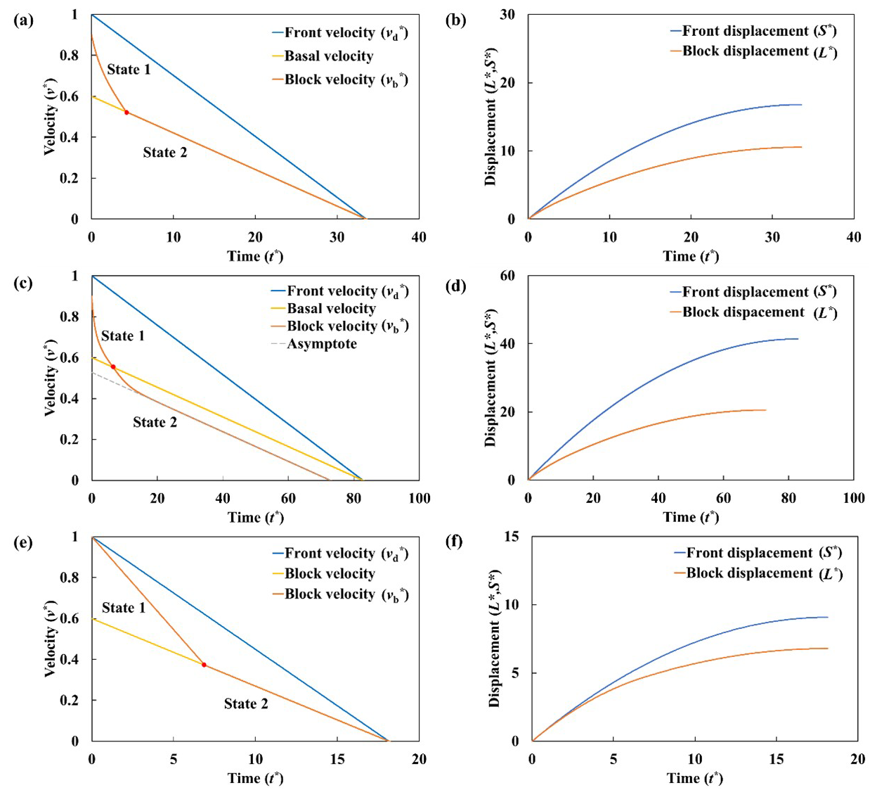
Figure 9 The velocity and displacement predicted by the models. Velocity time history of debris flow and block of (a) Model I, (c) and Model II, (e) Model III; displacement time history of debris flow and block of (b) Model I, (d) Model II, and (f) Model III. S^* is debris-flow deposition length (front displacement) and L^* is block displacement. Model I incorporates experimental data from Test 50-40, Model II utilizes data from Test 45-40, and Model III employs data from Test 53-40 (Table 2). Red points demarcate critical thresholds between State 1 and State 2.

At the start of State 2, the dynamic drag force is 0 (t^* = $t_{\mathrm{1}}^{*}$, Δv^* = 0), so only the earth pressure drives the block forward. If the earth pressure can compensate for the acceleration difference between the block and debris flow (K^* > $\left|G^{*}\right|$), the block will maintain the same velocity as the debris flow until the end of movement (Sect. S2 in Supplement). If not (K^* < $\left|G^{*}\right|$), the block velocity will be lower than the debris-flow velocity and approaches an asymptote.

When the earth pressure K^* is not considered (Model II) or is less than $\left|G^{*}\right|$ (case of Model I), the asymptote is parallel to the debris-flow velocity curve. The existence of an asymptote means that the velocity difference between the debris flow and block tends to be constant and the difference between the driving and resistance forces on the block reaches a steady state, indicating that the block motion tends to uniformly decelerate.

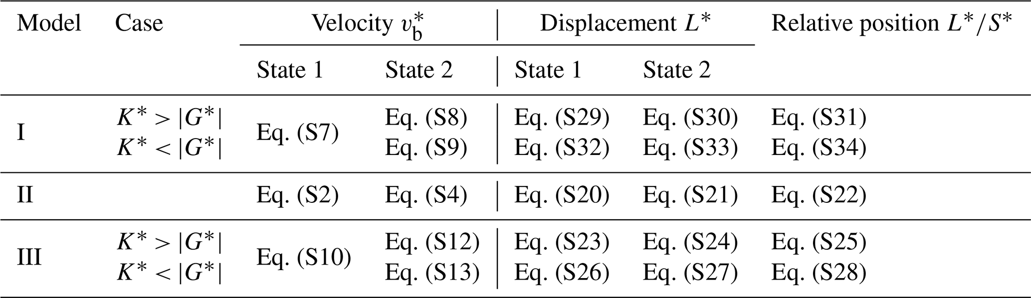
Based on the aforementioned constraints incorporated in the model solution framework, Table 3 systematically categorizes the computational approaches adopted for Models I–III. Details of the solutions can be found in the Supplement.

Table 3 Model classification and their corresponding solutions.

3.4.2 An example of the model solution

This section demonstrates the solution for Model II (Fig. 9c and d, 45 % concentration), as well as how to derive the velocity time history of block motion. When only the dynamic drag force is considered, the dimensionless momentum can be expressed as Eq. (16).

The block's movement process can be divided into two states:

State 1. Δv^* < 0. This state occurs during the initial states of debris flow displacing blocks, where both velocities are decreasing. Throughout this process, the block velocity persistently surpasses the debris-flow basal velocity (Fig. 9c, State 1), and the block velocity solution can be expressed:

$$\begin{array}{}\text{(18)}& \begin{array}{rl}& v_{\mathrm{b}}^{*}={\displaystyle \frac{\mathrm{1}}{n}}\left(\mathrm{1}-{\displaystyle \frac{G_{\mathrm{d}}^{*}}{\mathrm{2}}}{t}^{*}\right)-\sqrt{-{\displaystyle \frac{G^{*}}{D^{*}}}}\tan \\ & \left[-\sqrt{-G^{*}{D}^{*}}{t}^{*}+\arctan \left(\left(m-{\displaystyle \frac{\mathrm{1}}{n}}\right)\sqrt{-{\displaystyle \frac{D^{*}}{G^{*}}}}\right)\right]\end{array}\end{array}$$

According to Eq. (18), the dimensionless time ($t_{\mathrm{1}}^{*}$) when debris flow and block attain the same velocity (Red dot in Fig. 9c) is given by:

$$\begin{array}{}\text{(19)}& t_{\mathrm{1}}^{*}={\displaystyle \frac{\mathrm{1}}{\sqrt{-G^{*}{D}^{*}}}}\arctan \left(\left(m-{\displaystyle \frac{\mathrm{1}}{n}}\right)\sqrt{-{\displaystyle \frac{D^{*}}{G^{*}}}}\right)\end{array}$$

State 2. Δv^* > 0. This state occurs after the time $t_{\mathrm{1}}^{*}$ and block velocity is lower than debris-flow basal velocity (Fig. 9c, State 2), where the drag force acts as driving force to block. The solution can be expressed:

$$\begin{array}{}\text{(20)}& \begin{array}{rl}& v_{\mathrm{b}}^{*}={\displaystyle \frac{\mathrm{1}}{n}}\left(\mathrm{1}-{\displaystyle \frac{G_{\mathrm{d}}^{*}}{\mathrm{2}}}{t}^{*}\right)-\sqrt{-{\displaystyle \frac{G^{*}}{D^{*}}}}\tanh \\ & \left[\sqrt{-G^{*}{D}^{*}}{t}^{*}-\arctan \left(\left(m-{\displaystyle \frac{\mathrm{1}}{n}}\right)\sqrt{{\displaystyle \frac{D^{*}}{G^{*}}}}\right)\right]\end{array}\end{array}$$

The right side of Eq. (20) is the combination of debris-flow basal velocity and a hyperbolic tangent function (y = tanh (x)). As the independent variable x increases, tanh (x) is infinitely close to 1. Therefore, with the increase of dimensionless time $t_{\mathrm{1}}^{*}$, the dimensionless block velocity $v_{\mathrm{b}}^{*}$ tends to an asymptote, which is parallel to the dimensionless debris-flow basal velocity curve (Fig. 9c). The asymptote is given by:

$$\begin{array}{}\text{(21)}& v_{\mathrm{b}}^{*}{\mathrm{|}}_{\mathrm{asymptote}}={\displaystyle \frac{\mathrm{1}}{n}}\left(\mathrm{1}-{\displaystyle \frac{G_{\mathrm{d}}^{*}}{\mathrm{2}}}{t}^{*}\right)-\sqrt{-{\displaystyle \frac{G^{*}}{D^{*}}}}\end{array}$$

The displacement of the block is obtained by integrating its velocity. Due to the different solution forms of velocities in the two states, the block displacement can be divided into two states as well. By integrating Eq. (18) and applying the prescribed boundary conditions, the block displacement in State 1 (Fig. 9d) can be derived:

$$\begin{array}{}\text{(22)}& \begin{array}{l}{L}^{*}={\int }_{\mathrm{0}}^{t^{*}}\frac{\mathrm{1}}{n}\left(\mathrm{1}-\frac{G_{\mathrm{d}}^{*}}{\mathrm{2}}{t}^{*}\right)\mathrm{d}{t}^{*}\\ +{\displaystyle \frac{\mathrm{1}}{D^{*}}}\ln \left\{\cos \left[-\sqrt{-G^{*}{D}^{*}}{t}^{*}+\arctan \left(\left(m-{\displaystyle \frac{\mathrm{1}}{n}}\right)\sqrt{-{\displaystyle \frac{D^{*}}{G^{*}}}}\right)\right]\right\}\\ -{\displaystyle \frac{\mathrm{1}}{D^{*}}}\ln \left[\cos \left(\arctan \left(m-{\displaystyle \frac{\mathrm{1}}{n}}\right)\sqrt{-{\displaystyle \frac{D^{*}}{G^{*}}}}\right)\right]\end{array}\end{array}$$

Through integration of Eq. (20) under boundary conditions, the block displacement in State 2 (Fig. 9d) can be derived:

$$\begin{array}{}\text{(23)}& \begin{array}{l}{L}^{*}={\int }_{t_{\mathrm{1}}^{*}}^{T^{*}}\frac{\mathrm{1}}{n}\left(\mathrm{1}-\frac{G_{\mathrm{d}}^{*}}{\mathrm{2}}{t}^{*}\right)\mathrm{d}{t}^{*}\\ -\frac{\mathrm{1}}{D^{*}}\ln \left\{\cosh \left[-\sqrt{-G^{*}{D}^{*}}{T}^{*}+\arctan \left(\frac{\mathrm{1}}{n}\sqrt{-\frac{D^{*}}{G^{*}}}\right)\right]\right\}\end{array}\end{array}$$

where T^* is the stop time of block. The total block displacement throughout the kinematic process is obtained by superposition of the two displacement components. The normalized ratio $L^{*}/S^{*}$, defined as the block displacement relative to the debris flow deposition length, quantifies the block's relative position within the depositional zone:

$$\begin{array}{}\text{(24)}& \begin{array}{l}\frac{L^{*}}{S^{*}}=\frac{{\int }_{\mathrm{0}}^{T^{*}}\frac{\mathrm{1}}{n}\left(\mathrm{1}-\frac{G_{\mathrm{d}}^{*}}{\mathrm{2}}{t}^{*}\right)\mathrm{d}{t}^{*}}{{\int }_{\mathrm{0}}^{\frac{\mathrm{2}}{G_{\mathrm{d}}^{*}}}\left(\mathrm{1}-\frac{G_{\mathrm{d}}^{*}}{\mathrm{2}}{t}^{*}\right)\mathrm{d}{t}^{*}}\\ -\frac{G_{\mathrm{d}}^{*}}{D^{*}}\ln \left(\cos \left(\arctan \left(\left(m-\frac{\mathrm{1}}{n}\right)\sqrt{-\frac{D^{*}}{G^{*}}}\right)\right)\right)\\ -\frac{G_{\mathrm{d}}^{*}}{D^{*}}\ln \left(\cosh \right(\sqrt{-G^{*}{D}^{*}}{T}^{*}\\ -\arctan \left(m-\frac{\mathrm{1}}{n}\right)\left(\sqrt{-\frac{D^{*}}{G^{*}}}\right)\left)\right)\end{array}\end{array}$$

4 Model Validation and Discussion

The theoretical model initially derives velocity profiles for both debris flow and block (Fig. 9a, c, and e). Subsequent integration of these velocity time histories yields corresponding displacement trajectories (Fig. 9b, d, and f). Consequently, given known physical parameters of the debris flow and building fragment, the model predicts the relative position $L^{*}/S^{*}$. Under constant αFr², parametric variations in D^* and K^* generate the theoretical prediction curves for $L^{*}/S^{*}$ shown in Fig. 10.

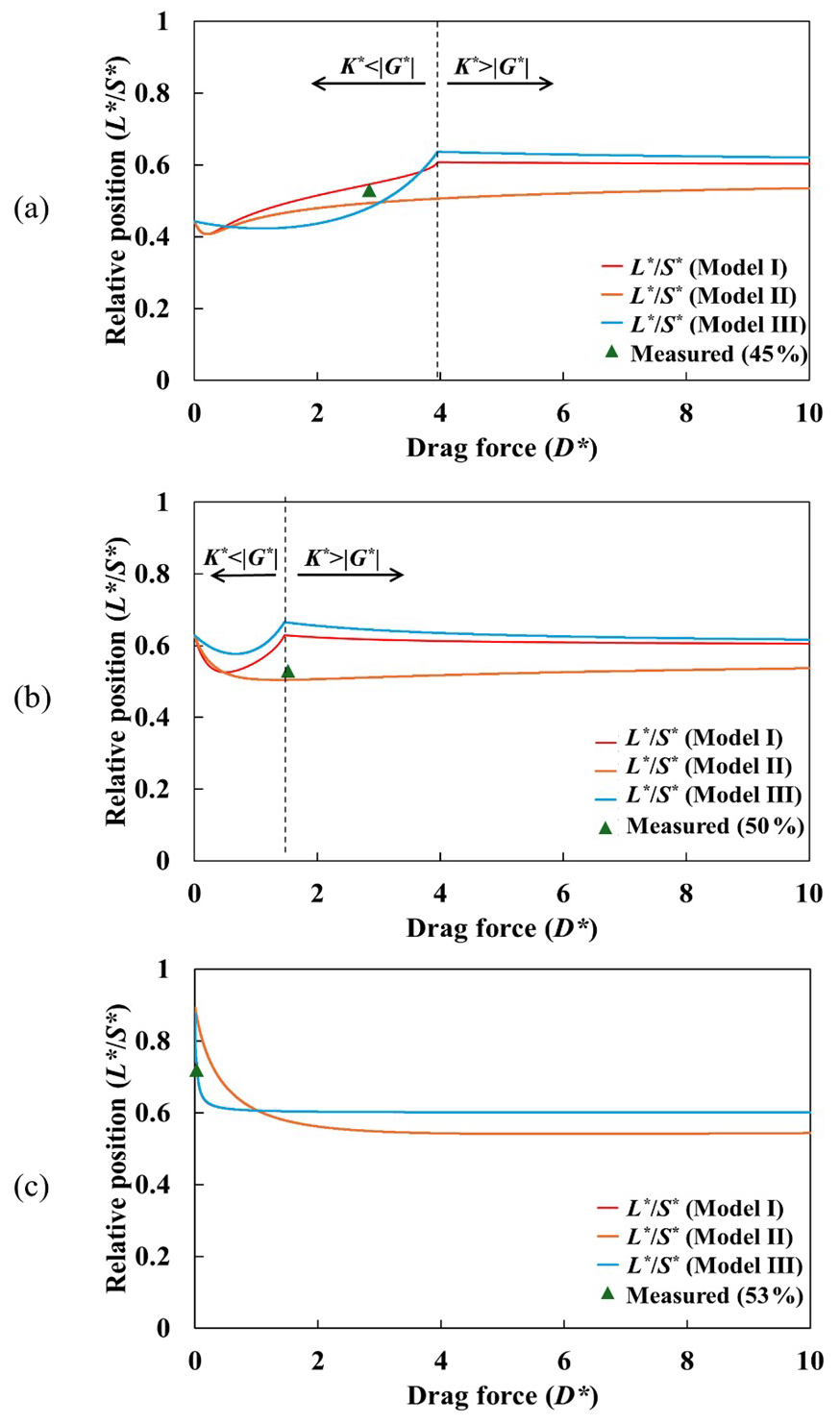
Figure 10 Verification of theoretical prediction against experimental results. (a) 45 % concentration; (b) 50 % concentration; and (c) 53 % concentration, where Model I and Model II exhibit congruent prediction trajectories.

4.1 Prediction for relative position ($L^{*}/S^{*}$)

The selection of parameters in the theoretical model is based on the physical characteristics of the experimental flume, the materials, and the measurements of the sensors (Table 4). In all experiments, the internal friction coefficient μ_d of debris flow solid particles is taken as 0.51, and the friction coefficient between debris flow solid particles and the bed is also 0.51. The friction coefficient μ_b between the block and bed is taken as 0.70. The drag coefficient C_d is assigned a typical value of 0.50, and the magnitude of the difference between the active and the passive earth pressure coefficient (k_p-k_a) amounts to 0.10.

Table 4 Physical parameters for model validation.

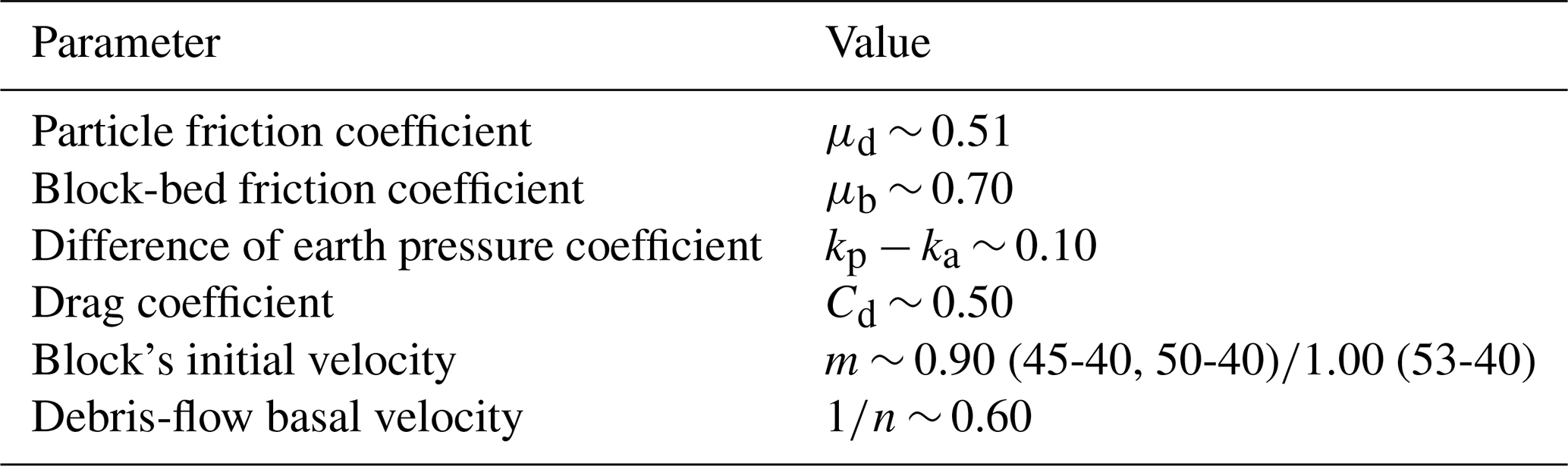
Figure 10 compares the theoretical predictions with the experimental results. The horizontal axis represents the magnitude of the force acting on the block. Since the drag force and earth pressure exhibit a linear relationship (αFr²) (Eq. 15), the horizontal axis can equivalently represent either drag force or earth pressure. Consequently, comparisons of theoretical predictions from three models are performed for experiments with three distinct solid-phase concentrations.

In the model classification, both Model I and Model III incorporate earth pressure considerations. During the model-solving process, the solutions can be categorized into two distinct classes based on the relative magnitudes of K^* and $\left|G^{*}\right|$. In Fig. 10, the left hand side of the dashed line represents scenarios where K^* < $\left|G^{*}\right|$, while the right hand side corresponds to situations where K^* > $\left|G^{*}\right|$. The critical distinction between these two cases lies in whether the block velocity in State 2 achieves synchronization with the debris flow velocity.

For Models I and III, when K^* < $\left|G^{*}\right|$, the normalized block position $L^{*}/S^{*}$ within the debris flow initially decreases and subsequently increases as the combined drag force and earth pressure intensify (Fig. 10). This phenomenon arises from the theoretical velocity prediction curve of the block (Fig. 9). In State 1, where the block's initial velocity is higher than that of the basal velocity of debris flow, both the drag force and earth pressure act as resistive forces. Larger magnitudes of these forces induce faster deceleration of the block. In State 2, the block's velocity falls below the basal flow velocity and asymptotically approaches a limited value. The difference between this asymptote and basal velocity curve is governed by the drag force and earth pressure: greater forces result in a smaller difference. Consequently, as the drag force and earth pressure increase, the block's velocity in State 2 gradually converges toward the debris flow velocity. Therefore, during State 1, the block's displacement exceeds the displacement of the debris flow front, whereas in State 2, the block's displacement becomes smaller than that of the flow front. The total block displacement is the sum of these two phases. The dynamic interplay between displacements in these two states governs the evolution of the relative position, ultimately leading to the non-monotonic trend (initial decline followed by an increase) in the $L^{*}/S^{*}$ curve when K^* < $\left|G^{*}\right|$.

In contrast, when K^* > $\left|G^{*}\right|$, the earth pressure ensures synchronization between the block's motion in State 2 and debris-flow basal velocity. Consequently, the block position depends on the duration of the deceleration phase in State 1. Higher drag force and earth pressure enhance deceleration, shortening the duration of State 1 and reducing the displacement difference between the block and debris flow front. Thus, the block position decreases monotonically with increasing drag force and earth pressure under K^* > $\left|G^{*}\right|$.

For Model II, no such critical boundary exists (Fig. 10), and the block velocity consistently remains higher than that of the basal flow velocity. The drag force modulates both (1) the rate at which the block asymptotically approaches its terminal velocity and (2) the magnitude of the difference between this asymptote and the basal flow velocity. The dynamic equilibrium between these two effects still induces a non-monotonic trend in the normalized accumulation position $L^{*}/S^{*}$, characterized by an initial decrease followed by an increase.

4.2 Model predictions vs. measured results

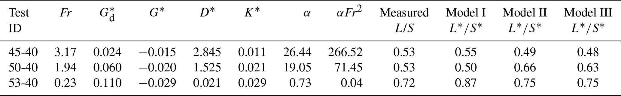
The αFr² of the 45 %-concentration experiment is 266.52 (Table 2), indicating that the dynamic drag force dominates the block movement. For the prediction of the 45 %-concentration experiment, the prediction of Model II is the closest (Fig. 10a). However, for the results of the 53 %-concentration experiment, the predictions of Model I and III almost overlap due to the negligible contribution of the dynamic drag force. The value of αFr² is 0.04, indicating that earth pressure plays a dominant role (Fig. 10c). For the 50 %-concentration experiment with αFr² = 71.45, the three theoretical predictions exhibit minor discrepancies (Fig. 10b). Neither of the two forces can be neglected, and Model I would provide appropriate prediction for the 50 %-concentration experiment. The relative deposition positions ($L^{*}/S^{*}$) for block across three solid concentrations yield: 0.53 (Test 45-40), 0.53 (Test 50-40), and 0.72 (Test 53-40), while the corresponding model predictions demonstrate close agreement: 0.49 (Test 45-40, Model II), 0.50 (Test 50-40, Model I), 0.75 (Test 53-40, Model III).

Experimental measurements establish the basal sliding velocity at 0.6 times the frontal velocity. The relative deposition positions ($L^{*}/S^{*}$ ∼ 0.49–0.75) from both experiments and theoretical prediction exhibit significant correlation to basal velocity (0.6).

4.3 Discussion

Conventional understanding posits that debris flows – as free-surface flows governed by gravitational and inertial forces – exhibit distinct regimes dictated by the dominance hierarchy between these forces, quantified through the Froude number (Fr). Consequently, the transport and deposition of blocks are presumed to demonstrate Fr-regime-dependent variability in relative deposition distance ($L^{*}/S^{*}$). Contrary to this paradigm, our theoretically derived curves for Models I–III exhibit remarkable congruence, showing negligible divergence across Fr regimes (Fig. 10).

Analysis of velocity time histories under varying solid concentrations reveals a universal characteristic: irrespective of whether transport is dominated by earth pressures or dynamic drag forces, block velocities invariably converge toward basal flow velocities at the block's equilibrium position (Fig. 9). This kinematic convergence results in deposition distances that remain invariant to gravitational-inertial dominance transitions. The basal sliding velocity exerts a dominant control on block position, fundamentally governing the prediction envelope of $L^{*}/S^{*}$. Specifically, adopting a basal sliding velocity of 0.6v_d (where v_d is frontal velocity) yields theoretical and experimental $L^{*}/S^{*}$ values consistently converging at 0.6, demonstrating the control of basal sliding velocity on the position of building block. This practical finding enables emergency responders to predict final block position (and the trapped victims) solely from debris-flow velocity profiles (basal sliding velocity).

5 Conclusions

• 1.

  Quantitative experimental measurements reveal substantial divergence in flow regimes across three solid concentrations (45 %, 50 %, and 53 %), manifested through different flow velocities, depths, and degrees of liquefaction. Critically, high-speed imaging analysis confirms pervasive basal sliding phenomena, with measured basal velocities attaining ≈ 0.6 times the frontal flow velocity. Based on the data from the IMU, the block exhibits impulsive acceleration characteristics during the initial contact. IMU-derived kinematic data demonstrate block initial velocity up to 0.9–1.0 times the frontal flow velocity upon initial contact, followed by progressive deceleration during burial.

• 2.

  This study proposes an analytical model to predict the relative position ($L^{*}/S^{*}$) of building fragment in debris-flow deposition, which is governed by several dimensionless numbers (Fr, $G_{\mathrm{d}}^{*}$, G^*, D^*, K^*). These dimensionless parameters consider various physical processes, including terrain characteristics (slope, basal friction), incoming-flow characteristics (degree of liquefaction, flow inertia, static load), block characteristics (relative density with debris flow), drag of debris flow, and active and passive earth pressures. Based on the flow regime of debris flows and the dominant force of the process, we categorize the models into three types: Model I governed by the combined action of dynamic drag force and earth pressure, Model II dominated by dynamic drag force, and Model III dominated by earth pressure.

• 3.

  Based on a comparative analysis of model predictions and experimental results, we find that the position of blocks within the depositional zone of debris flows is dominated by basal sliding effects. Regardless of the flow regime, the block velocity consistently tends to approach the basal flow velocity of the debris flow. Consequently, the relative position of blocks in the deposition converges toward the ratio of the basal flow velocity to the flow front velocity.

This study has significant practical implications for post-disaster emergency rescue, particularly in locating the positions of buried buildings within debris flow deposits. Moreover, findings of this study could have practical implications for locating the position of other objects (e.g., cars) in rock avalanches or snow avalanches. Nevertheless, substantial simplification has been made to achieve the above findings. Specially, the modelled building block lies in a 2D deposition zone, rather than a deposition fan. By modelling a high-density flat block contacting the channel bed, the rotation along the flow direction is constrained. In terms of the modelled debris flow, the mono-sized spherical particles mixed with Newtonian fluid is an idealization of prototype debris flows. The analytical model is built on a uniform deceleration model, which only reflects a specific scenario on the deposition area. Only the prediction of a single building fragment position in debris flow deposition is provided, rather than the distribution range of building fragments, which is beyond the capacity of deterministic analytical models. Further study, including large-scale experiments and well-calibrated numerical modelling, is needed to shed light on this complicated problem.

Appendix A: Notation

α	Coefficient combining drag coefficient, earth pressure coefficients, degree of liquefaction, and relative block height
λ	Degree of liquefaction
μb	Friction coefficient between block and bed
μd	Friction coefficient between debris flow and bed; Internal friction coefficient
ρ*	Relative density
ρb	Density of block
ρd	Density of debris flow
θ	Slope angle
θ0	Slope angle of the upstream section
A	Frontal area of block exposed to flow
B	Block dimension in y direction (width)
Cd	Drag coefficient
D*	Dimensionless number related to drag force
Fr	Froude number
g	Gravitational acceleration
G*	Dimensionless acceleration difference between debris flow and block
Gb	Equivalent acceleration of block
$G_{\mathrm{b}}^{*}$	Dimensionless equivalent acceleration of block
Gd	Equivalent deceleration of debris flow
$G_{\mathrm{d}}^{*}$	Dimensionless equivalent deceleration of debris flow
h	Height of block
h0	Frontal depth of the upstream incoming debris flow
H	Flow depth of debris flow
k	Earth pressure coefficient
ka	Active earth pressure coefficient
kp	Passive earth pressure coefficient
K*	Dimensionless number related to earth pressure
L	Block displacement
L*	Dimensionless block displacement
m	Ratio of block initial velocity to frontal debris flow velocity
n	Ratio of basal sliding velocity to frontal flow velocity
S	Debris-flow deposition length
S*	Dimensionless debris-flow deposition length
t	Time
t*	Dimensionless time
$t_{\mathrm{1}}^{*}$	Dimensionless time when block and basal flow velocities become equal
T*	Dimensionless stop time of block
v0	Frontal velocity of upstream incoming debris flow
v1	Equivalent upstream inflow velocity
vb	Velocity of block
$v_{\mathrm{b}}^{*}$	Dimensionless velocity of block
vd	Velocity of debris flow
$v_{\mathrm{d}}^{*}$	Dimensionless velocity of debris flow
Δv	Difference between basal sliding velocity and block velocity
Δv*	Dimensionless difference between basal sliding velocity and block velocity
Vb	Volume of block