the Creative Commons Attribution 4.0 License.
the Creative Commons Attribution 4.0 License.
 | 12 Jun 2026
Hybrid forest disturbance classification using Sentinel-1 and inventory data: a case-study for Southeastern USA
Franziska Müller
Laura Eifler
Felix Cremer
Pieter Beck
Gustau Camps-Valls
Ana Bastos
Forest ecosystems are increasingly threatened by disturbances such as fires, droughts, storms, and insect and pathogen outbreaks. Accurate and timely disturbance mapping is essential for understanding their dynamics and informing mitigation strategies to combat widespread forest decline. Traditional inventories, such as the U.S. Forest Service’s Insect and Disease Survey (IDS), provide detailed information on biotic and abiotic disturbances; however, they have varying coverage and inherent uncertainties in the location, extent, and timing of disturbances due to data-collection constraints. Other approaches, such as satellite remote sensing, can, in principle, overcome some of these challenges by providing large-scale coverage and continuous spatio-temporal observations. However, robust disturbance classification algorithms need to be developed, which in turn require good-quality labels.
We present a novel approach for refining disturbance classification labels by combining IDS with Sentinel-1 radar backscatter change detection to produce a new reference dataset, Sentinel-1 Disturbance Mapping (S1DM). The disturbed patches identified by Sentinel-1 are typically located within 200–330 m of IDS locations and generally agree on disturbance timing. Sentinel-1 tends to detect bark beetle disturbances up to 2 years earlier than IDS, and some defoliator events are also detected 1 year prior to IDS. When statistically examined against manual labels from high-resolution images from PlanetScope, we found that S1DM performed better than IDS for wind and bark beetle disturbances, but not for defoliators. For bark beetle disturbances, S1DM improves the median Intersection over Union from 0.007 to 0.076, an absolute gain of 6.9 % over IDS.
By integrating spatial and temporal information on disturbance occurrence from Sentinel-1 change detection with information on the corresponding disturbance agent from IDS, S1DM provides a high-quality forest disturbance reference dataset for developing remote sensing forest classification models.
Our approach highlights the benefits of combining satellite-based remote sensing with traditional aerial survey data, reducing aerial survey costs while providing a scalable method adaptable to various regions.
- Article
(5209 KB) - Full-text XML
- BibTeX
- EndNote


Forests play a critical role in mitigating climate change by acting as carbon sinks, storing carbon in their biomass (e.g., leaves and roots) and in the soil (Pan et al., 2024). Recent observations suggest that climate change is likely contributing to recent tree mortality events (Hartmann et al., 2022; Bauman et al., 2022; Hammond et al., 2022). Tree mortality is driven by a combination of natural disturbances (e.g., wildfires, storms, insects and pathogens) (Schuldt et al., 2020; Senf et al., 2020; Hicke et al., 2016, 2020; Kautz et al., 2017; Anderegg et al., 2015) and changes in land management. Both factors can undermine forests' capacity to act as carbon sinks (Winkler et al., 2023; Harris et al., 2016, 2012; Nabuurs et al., 2013; Korosuo et al., 2023). In some cases, disturbances can temporarily convert forests into carbon sources, thereby amplifying global carbon emissions (Kurz et al., 2008; Hicke et al., 2012; European Environment Agency (EU body or agency), 2024; Byrne et al., 2024).
As climate change accelerates, the frequency and intensity of disturbances – including wildfires (Canadell et al., 2021a; Jones et al., 2022), storms (Senf and Seidl, 2021b), and insects and pathogens (Graziosi et al., 2020; Seidl et al., 2017) – are increasing and heightening forest vulnerability (Forzieri et al., 2021; Altman et al., 2024). These changes in disturbance regimes threaten vital ecosystem services, including carbon sequestration, water regulation, soil protection, and biodiversity conservation, which are essential for environmental and societal well-being (McDowell et al., 2020; Richter et al., 2022; Trumbore et al., 2015; Seidl et al., 2014; Thom and Seidl, 2016).
Despite the growing impact of forest disturbances on ecosystems worldwide, understanding their dynamics remains challenging due to the uneven global distribution of forest disturbance data (Kautz et al., 2017). A common approach to monitoring forest disturbances is through inventories, in which trained surveyors document disturbances across large forested areas (McDowell et al., 2020; Coleman et al., 2018). However, the quality and extent of reporting vary significantly across regions. For example, FAO (2020) shows that the availability of disturbance reports (i.e., data availability) differs considerably by disturbance type and geographic region. Between 2002 and 2016, data availability for insect disturbance reports covered 98 % of forested areas in North and Central America and 86 % in Europe, but only 45 % in Asia (FAO, 2020). Coverage of reports on severe weather disturbances included 50 % of forest areas in North America, 86 % in Europe, and just 8 % in Asia. These disparities highlight the uneven spatial coverage and inconsistencies in the types of natural disturbances recorded in inventory data.
Although many inventories have limitations in spatial and temporal coverage, several notable efforts provide more comprehensive datasets. These include the Forest Service’s Insect & Disease Detection Surveys (IDS) and the Canadian Forest Service’s National Forestry Database (NFD), both of which rely on aerial surveys to monitor large-scale disturbances such as insects, diseases, wildfires, and droughts. In Europe, critical datasets on forest damage from insects and diseases include the Database of Forest Disturbances in Europe (Patacca et al., 2021, DFDE), the Dataset of Wind Disturbances in European Forests (Forzieri et al., 2020, FORWIND), and the Database of European Forest Insect and Disease Disturbances (Forzieri et al., 2023, DEFID2), with variable coverage in space and time. However, human errors, low sampling frequency, spatial inaccuracies, and inconsistent collection methods across countries affect inventory data, creating spatial biases, making dataset aggregation challenging, and preventing broader harmonized assessments (Forest Service U.S. Department of Agriculture, 2024; McConnell, 2000; Coleman et al., 2018; Eifler et al., 2026; Forzieri et al., 2023).
Because traditional forest inventory datasets are limited and unevenly distributed (Kautz et al., 2017; FAO, 2020), remote sensing has emerged as a crucial alternative for monitoring forest disturbances. Remote sensing provides spatially and temporally consistent and cost-effective solutions for tracking forest conditions across large areas and extended periods. Several long-running satellite missions and sensors support these efforts, including MODIS (operational since 1999; Justice et al., 1998), the Landsat program (initiated with Landsat 1 in 1972 and most recently continued with Landsat 8 launched in 2013; Markham and Helder, 2012; Hansen and Loveland, 2012), and the Sentinel satellite fleet operated by ESA, with multiple satellite missions launched between 2014 and 2025 (ESA, 2015). Satellite time series of vegetation-related variables have allowed the detection of forest disturbances, monitor forest cover changes (Hansen et al., 2013; Popp et al., 2020), and assess disturbance and regrowth patterns caused by wildfires, drought, and logging (Seidl and Turner, 2022; Senf et al., 2019; Heinrich et al., 2021; Senf and Seidl, 2021a), leading to global disturbance maps for these agents (Chuvieco et al., 2018; Vicente-Serrano et al., 2013; Curtis et al., 2018). In contrast, comprehensive mapping and classification of other disturbance agents, such as wind-throw or insects and pathogens outbreaks, remains limited, despite their known potential to cause substantial changes to forest ecosystems (Harris et al., 2016; Kautz et al., 2018, 2017). Global satellite-based estimates of forest disturbances caused by windstorms or biotic agents, such as insect outbreaks, do not currently exist (FAO, 2020; Kautz et al., 2017). This is primarily due to the difficulty in detecting smaller or slower disturbances – like droughts or subtle, temporary impacts from defoliators – where trees may recover after the event, making the damage harder to capture (McDowell et al., 2015). However, regional case studies have shown that it is possible to detect individual wind-throw events, bark beetle outbreaks, and defoliator attacks using existing satellite sensors such as Sentinel-2, Landsat, or MODIS (Negrón-Juárez et al., 2018; Senf et al., 2015; Eklundh et al., 2009; Meddens et al., 2012). Optical sensors provide extensive multispectral data, enabling the detection of disturbance hotspots, canopy health decline, and recovery across large areas (Senf and Seidl, 2018; Candotti et al., 2022; Hall et al., 2016; Hicke et al., 2016). However, their reliance on cloud-free conditions and their limited ability to detect subtle disturbances, such as those induced by biotic stress or drought (McDowell et al., 2015) – can limit the range of their applications.
An alternative solution is provided by Radio Detection and Ranging (RADAR) and Light Detection and Ranging (LiDAR) sensors, which offer information on structural changes. Radar imaging at high temporal and spatial resolution provided by the Sentinel-1 mission has shown potential for detecting different types of forest disturbances in regional case studies, including windthrows (Rüetschi et al., 2019), defoliation events (Bae et al., 2022), and bark beetle infestations (Dalponte et al., 2024). Since radar operates in the microwave range, it is not affected by cloud cover, making it particularly useful for continuous monitoring in all weather conditions. Furthermore, radar backscatter is sensitive to changes in vegetation water content (Konings et al., 2021), and thus potentially more suitable to detect early states of slow-onset disturbances, such as insect outbreaks, and changes in canopy structure, driven, for example, by windthrow events.
Increasingly, remote sensing studies use data-driven approaches (e.g., Artificial Intelligence) to detect, map, and classify forest disturbances, demonstrating their ability to capture complex spatiotemporal patterns (Andresini et al., 2024; Bárta et al., 2021; Hawryło et al., 2018; Gibson et al., 2020). The effectiveness of these models depends on high-quality reference data, as accurate ground-truth labels are essential for training and validating disturbance detection algorithms. This data-hungry approach creates a bottleneck because labeling forest disturbances requires extensive labor and expertise to distinguish agents such as insects, drought, or biotic stress.
In this study, we develop a hybrid forest disturbance benchmark dataset that integrates satellite observations with disturbance inventory data, focusing on three key disturbance types: bark beetles, defoliators, and wind. This choice is motivated both by their ecological importance (Seidl et al., 2017; Hicke et al., 2020; US Forest Service, 2013; Heaton et al., 2023) and the known challenges and persistent gaps in remote sensing-based classification of these disturbance types (McDowell et al., 2015; Kautz et al., 2017; Schleeweis et al., 2020). For example, bark beetles have killed approximately 3.8 billion trees in western North America between 1997 and 2018 (Hicke et al., 2020), and the defoliating gypsy moth (Lymantria dispar) has affected over 21.5 million ha in the northeastern United States from 1924 to 2015 (Karel and Man, 2017). Insect disturbances are responsible for substantial carbon losses (10 ± 1.3 Tg C yr−1), comparable to those attributed to fire (7 ± 1.0 Tg C yr−1) in the United States (Harris et al., 2016). Wind disturbances, while sparse in time, can be catastrophic, as exemplified by Hurricane Hugo, which damaged around 1.8 million ha of forest in South Carolina (Heaton et al., 2023), and storms have been associated with carbon losses of up to 5 ± 0.7 Tg C yr−1 during the period 2006–2010 (Harris et al., 2016). Here, we aim to support advances in wind and insect disturbance classification by combining C-band Synthetic Aperture Radar (SAR) data from Sentinel-1 with inventory-based information. As the SAR signal is sensitive to structural and moisture changes that are not easily captured by optical sensors and visual inspection, and can penetrate through clouds, and given Sentinel-1's spatially and temporally continuous information, this approach allows for refining inventory-based disturbance maps and reducing spatial and temporal uncertainties. To support validation and quality control, we additionally incorporate a Tree Canopy Cover (TCC) dataset, which provides independent high-resolution estimates of forest canopy cover, and use high-resolution Planet imagery with manual labeling to assess whether this approach leads to significantly improved disturbance detection.
2.1 Study area
This study focuses on a specific region within the United States – the southeastern area classified by the United States Department of Agriculture (USDA) as Region 8 (Fig. 1). This region spans approximately 73 million hectares of forest across 13 states, with a wide variety of forest types and disturbance regimes, making it an ideal area for studying large-scale forest dynamics and disturbances.
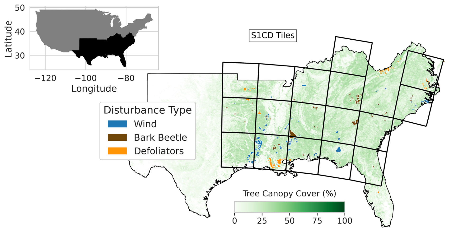
Figure 1Spatial overview of USDA Region 8, with detailed disturbance and canopy cover data. The inset map (top left) shows the location of Region 8 within the United States, highlighted in black. The main map displays the outline of Region 8, with 2015 Tree Canopy Cover (TCC) shaded in green, representing the percentage of canopy cover. Overlaid on the TCC map are visually enlarged disturbance patches for three selected disturbance types (wind, bark beetles, and defoliators) based on preprocessed Insect and Disease Survey (IDS) data (Forest Service U.S. Department of Agriculture, 2024) from 2016 to 2020, showing disturbances under 15 km2 in size. The grid outlines represent the spatial coverage of the Sentinel-1 Change-Detection (S1CD) dataset (Cremer et al., 2020; this study). This figure illustrates the spatial distribution of tree canopy cover, disturbance events, and the S1CD grid tiles used for analysis across Region 8.
The forests in this vast region exhibit high diversity, with a mix of broadleaf and coniferous species flourishing across a spectrum of climate conditions. From the humid subtropical zones of coastal and lowland areas to the temperate mixed forests of higher elevations, these ecosystems support a rich array of ecological functions and forest management practices, each uniquely shaped by the interplay of climate, topography, and species composition. In the Interior Highlands and Interior Plains (the central and northern parts of the study area), low-elevation mountains and flat terrain are dominated by deciduous species, including White Oak (Quercus alba), Red Oak (Quercus rubra), and various Hickory species (Carya spp.). In contrast, the Atlantic Plains (southern regions), with their wetter conditions and extensive wetlands, support deciduous species like Baldcypress (Taxodium distichum), Water Tupelo (Nyssa aquatica), and Sweetgum (Liquidambar styraciflua). The Appalachian Highlands, with higher elevations and cooler climates, contribute to further diversity, featuring mixed species such as Sugar Maple (Acer saccharum), Yellow-poplar (Liriodendron tulipifera), and Eastern White Pine (Pinus strobus). A comprehensive species list is available in Appendix Table A1 and the US Forest Service Map for Tree Species in the Southeastern United States (Woudenberg et al., 2010).
The study region spans a broad climatic gradient typical of the southeastern United States. Mean annual temperatures generally range from approximately 12–14 °C in the northern and higher-elevation areas to 20–22 °C in the southern coastal and lowland regions. Annual precipitation is relatively high across the region, typically ranging from about 1100 to 1600 mm, with higher rainfall in coastal zones and the Appalachian Highlands. The region is characterized by humid subtropical conditions in the south and east, transitioning to more temperate climates at higher elevations and latitudes. In addition, large portions of the study area lie within the North Atlantic hurricane track, making the region frequently exposed to tropical storms and hurricanes that bring strong winds and heavy rainfall, particularly in coastal and lowland areas. These climatic gradients and extreme weather events strongly influence forest composition, productivity, and disturbance regimes, including insect outbreaks, storm damage, and drought-related stress.
This diverse forest composition, with varying ecological zones and management strategies – from conservation-driven national parks to privately managed timberlands – creates a complex landscape in which disturbances manifest in various ways across the region. We do not focus on a single tree species or management practice, but instead conduct a complex yet holistic analysis of disturbances applicable to a wide range of forest types.
To analyze forest disturbances affecting this region, we use three key datasets: the Insect and Disease Survey (IDS), Sentinel-1 Change-Detection (S1CD), and Tree Canopy Cover (TCC). These datasets form the foundation of our analysis, providing complementary information on forest disturbances, structural changes in canopy cover, and the presence/absence of trees. Table 1 summarizes their key characteristics, with further details discussed in the following sections.
Throughout this paper, we use consistent terminology to refer to spatial representations of disturbances. We use the term polygon to describe the vector-based geometries in the IDS dataset, reflecting the original IDS data format and nomenclature. In contrast, patch refers to the disturbance outlines derived from the S1CD dataset in raster format, which are later converted to polygons for analysis.
Table 1Key characteristics of the datasets used in this study: the Insect and Disease Survey (IDS), Sentinel-1 Change Detection (S1CD), Tree Canopy Cover (TCC), and Planet imagery. The table summarizes the information content, data format, spatial resolution, temporal availability, and role of each dataset in the analysis.
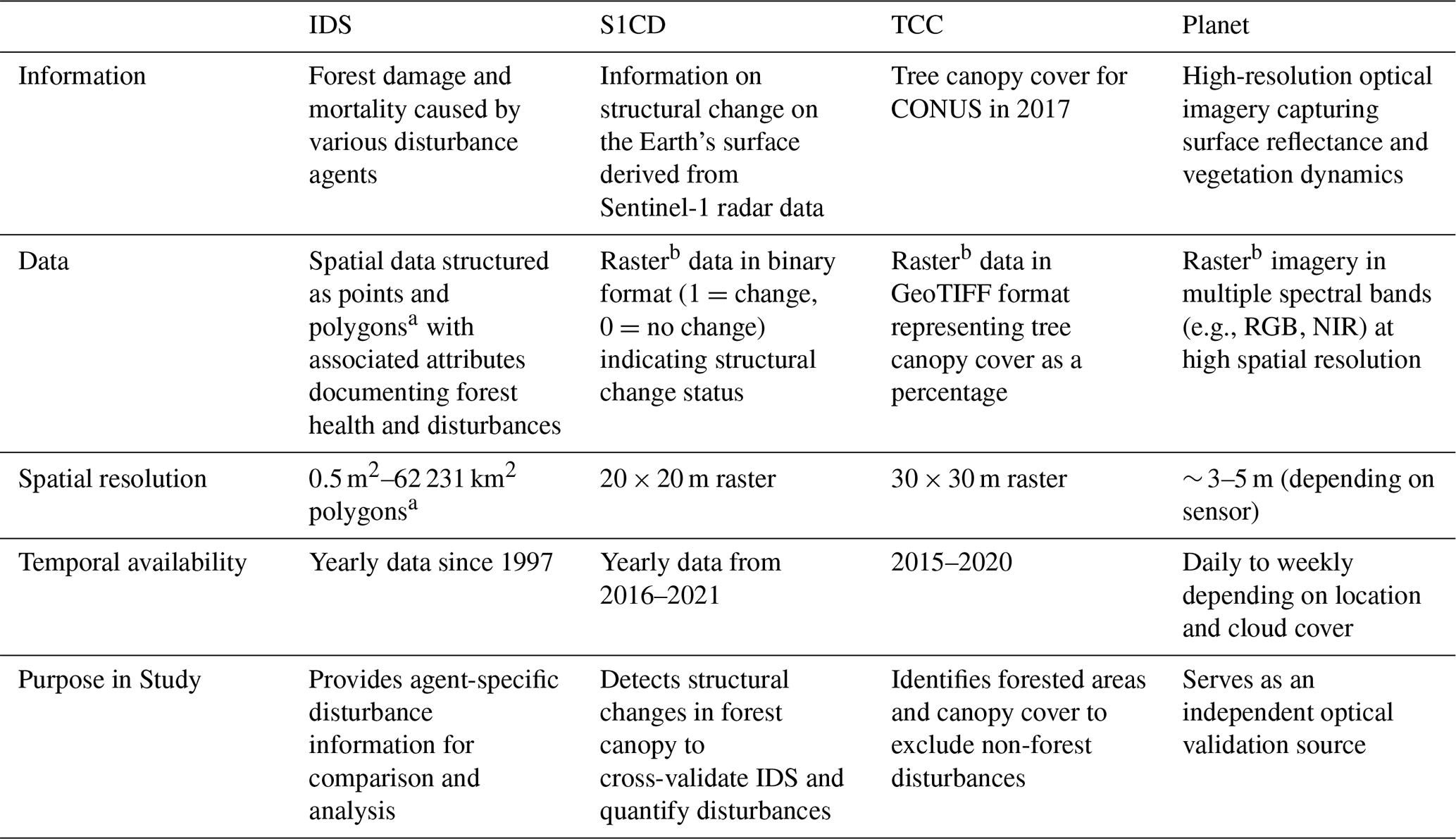
a Polygons are vector-based, representing features with precise boundaries using points, lines, and polygons. b Raster data is pixel-based, representing space as a grid of cells with values. A disturbance (single pixel or multiple pixels) is referred to as a patch.
2.2 Insect and Disease Detection Survey (IDS)
The Insect and Disease Survey (IDS), is conducted by the United States Department of Agriculture (USDA) Forest Service (Forest Service U.S. Department of Agriculture, 2024) and monitors forest damage and mortality resulting from various disturbance agents. Since 1997, the IDS has monitored disturbance agents across the United States and its territories, including fires, wind, bark beetles, defoliating insects, and fungal diseases.
Disturbances are mapped as geo-referenced polygons that represent areas where damage was observed, though not all trees within a polygon are necessarily affected. For each polygon, surveyors record a range of attributes (USDA Forest Service, 2022, 2005); those used in this study include the affected tree species, the causal agent, the survey year, the damage type (e.g., mortality, defoliation percentage, crown dieback, branch breakage, or other non-mortality damage), and the severity class, expressed as the percentage of live and damaged trees within the polygon (Very Light: 1 %–3 % through Very Severe: >50 %). For the causal agents, the IDS database includes more than 1000 fine-grained disturbance agent codes, which are hierarchically organized into 28 broader categories. To reduce interpreter uncertainty and ensure analytical consistency, the 63 bark beetle and 210 defoliator agents were aggregated to their broader categories in IDS (Table A5), while wind, formally a subgroup of the abiotic damage category, was considered separately due to its distinct disturbance characteristics. The resulting aggregated disturbance categories used here, namely wind, bark beetles, and defoliators, are referred to as DCA_ID.
In our study region 8, the IDS recorded a total of 2992 disturbances from 2017 to 2020. Bark beetle outbreaks were the most frequent (1177 events), followed by wind (478) and defoliators (213). Annual disturbance counts varied considerably, from 210 events in 2017 to 1374 in 2018. The total disturbed area also varied by type and year: defoliation affected the most significant area in 2018 (119 km2), while wind caused the largest area loss in 2020 (343 km2). Bark beetle outbreaks were widespread but generally affected smaller areas per event, whereas wind and defoliation events often covered larger contiguous areas.
IDS data is collected primarily through aerial detection surveys (ADS) conducted by trained professionals. While ground-based surveys are used to verify specific disturbances or assess localized events, ADS provides the most effective method for large-scale disturbance monitoring, especially for extensive forest areas (Coleman et al., 2018).
Although mapping disturbances across large areas, such as the United States, would be impossible without ADS, this method presents several challenges. Surveyors must contend with factors such as the aircraft's high speed (approximately 100 mph), the angle of observation, and the complexity of detecting disturbances in a constantly changing landscape. Despite the aid of geo-referencing tools, these challenges often result in imprecise delineations, sometimes including healthy trees or non-forest areas, especially during large-scale outbreaks when time constraints limit accuracy (Backsen and Howell, 2013; Coleman et al., 2018; Kautz, 2014). This uncertainty is explicitly acknowledged in the IDS protocol: for each mapped polygon, the attribute “percent affected” provides a standardized estimate of the proportion of trees within the area that the identified disturbance agent impacts. Although quick decisions are necessary during ADS, surveyors generally correctly attribute disturbance agents, making false positives (Type I errors, where a disturbance is recorded but did not actually occur) rare. However, compound disturbance events, i.e., events that occur in quick succession, simultaneously, or that trigger one another, can create overlapping effects. For example, a drought may increase bark beetle activity, or storms may be followed by bark beetle outbreaks. These overlapping influences make it difficult to disentangle individual agents, sometimes leading to false negatives (Type II errors, where a real disturbance impact is missed or misattributed), resulting in specific disturbance effects going unnoticed (Coleman et al., 2018).
Biotic disturbances, such as defoliators and bark beetles, occur within specific temporal windows of activity that must be captured accurately through timely ADS. However, weather, funding, and surveyor availability can delay flights, preventing surveys from being conducted during these critical windows. As a result, disturbances may be missed or monitored at suboptimal times (McConnell, 2000). Additionally, some disturbances may not be detectable until after they occur, resulting in a time lag between the actual disturbance and its detection, as seen with bark beetles (Kautz, 2014). Due to the large areas that must be covered, flight patterns often change from year to year, and some regions may not be surveyed at all in a given season. Survey coverage follows specific flight paths rather than encompassing every forested area, and the extent of the flown area is made available annually as a geodatabase. This information is particularly important for interpreting records from 2020 and 2021, when COVID-19 restrictions limited aerial surveys and protocols shifted toward greater use of remote sensing. This variability in flight coverage can introduce biases and inconsistencies, particularly in disturbance attribution, since areas may not always be flown at the optimal time for detecting damage.
Given these spatial and temporal uncertainties, ground verification is used to validate aerial survey data and investigate anomalies. However, due to time, funding, and data volume constraints, less than 1 % of the mapped polygons are verified annually (Coleman et al., 2018).
Despite these challenges, the IDS dataset offers invaluable insights into large-scale forest disturbances. With nearly 27 years of data since 1997, it provides a unique perspective for analyzing short- and long-term disturbance patterns. Another strength is its broad spatial extent, spanning the entire United States, including remote and difficult-to-reach areas where ground-based monitoring is impractical. Importantly, it covers both public and private lands, thereby reducing biases related to forest management practices, land ownership, and tree species. The dataset captures a wide range of disturbance agents, including fires, wind, bark beetles, defoliating insects, and fungal diseases, along with detailed metadata on damage severity, affected tree species, and other critical factors. While it has limitations in spatial and temporal accuracy and verification, its extensive coverage, variety of disturbance agents, and detailed metadata make it an indispensable tool for understanding forest dynamics and disturbance patterns across the United States.
2.3 Tree Canopy Cover (TCC)
To focus exclusively on forested areas, we used the Tree Canopy Cover dataset (NLCD TCC; Housman et al., 2025) from the Forest Service of the U.S. Department of Agriculture. The data is available for CONUS for the years 2015–2020 at a 30 m × 30 m spatial resolution and used to distinguish forested areas from non-forest areas in the study.
2.4 Sentinel-1 backscatter data
Here, we aim to produce an independent, satellite-based dataset of forest disturbances using Sentinel-1 C-Band Synthetic Aperture Radar (SAR) data (Torres et al., 2012). Unlike optical sensors, SAR is unaffected by cloud cover or sunlight, allowing consistent, year-round monitoring at high temporal (12 d) and spatial (20 m × 20 m) resolution (Torres et al., 2012). The C-band radar (5.4 GHz, 5.6 cm wavelength), and particularly the Vertical transmit/Horizontal receive (VH) backscatter, is sensitive to canopy water content and structure (Wu et al., 2025; Huang et al., 2018), making it particularly well-suited to capture the three disturbance types that are the focus of this study. Bark beetle outbreaks reduce canopy moisture (Kautz et al., 2024), defoliators minimize leaf area and wind can remove branches or uproot entire trees, creating gaps and altering canopy structure – all of which can be detected by radar even when foliage remains green to human observers or spectral satellite sensors. Bark beetle outbreaks reduce canopy moisture (Kautz et al., 2024), defoliators minimize leaf area (Woodman et al., 2021; Helbig et al., 2021), and wind can remove branches or uproot entire trees (Mitchell, 2013), creating gaps and altering canopy structure – all of which can be detected by radar even when foliage remains green to human observers or spectral satellite sensors (Tanase et al., 2019).
Here used the VH data from the Sentinel-1 Backscatter Datacube produced by Wagner et al. (2021), extracted for 17 tiles covering our study region for the period 2016–2021 (see Fig. 1, Table A2). These data are orthorectified and topographically corrected, and provided on a 20 m × 20 m resolution grid in the EQUI7 grid system (Bauer-Marschallinger et al., 2014).
2.5 PlanetScope
We used Planet data in this study to manually validate the new dataset and statistically assess whether the methodology produced a significantly improved product compared to IDS. We acquired the PlanetScope imagery through the Planet Education and Research (E&R) Standard Program (PBC, 2025), which provides limited, non-commercial access to PlanetScope and RapidEye imagery for university-affiliated students, faculty, and researchers. Access to the program requires a valid university email address; in this case, imagery was obtained using an institutional email from the University of Leipzig, granting permission to use PlanetScope data for research purposes.
PlanetScope imagery consists of high-resolution optical data acquired from a constellation of CubeSats, with a nominal daily revisit, although actual coverage can be affected by clouds, acquisition gaps, or satellite scheduling. Each scene has a spatial resolution of approximately 3–5 m and includes four spectral bands: Blue, Green, Red, and Near-Infrared, suitable for monitoring vegetation and detecting forest disturbances.
RapidEye imagery complements PlanetScope with 5 m multispectral data, including a Red Edge band in addition to Blue, Green, Red, and Near-Infrared, enhancing vegetation health assessment. Both datasets are orthorectified and radiometrically calibrated, allowing consistent analysis over time and across study areas. Their high temporal frequency and spectral information make them particularly useful for tracking fine-scale forest disturbances and vegetation dynamics.
Figure 2 outlines the key steps used to preprocess, intersect, and analyze the data. These steps are described in more detail below. We performed all data processing using Python (see Code Availability).
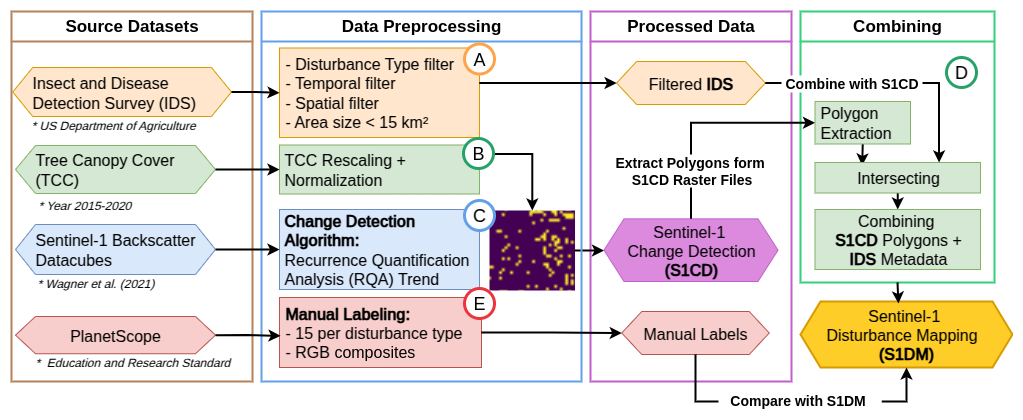
Figure 2Workflow illustrating the methodology used to create the radar-enhanced dataset and analyze the results. Rectangles represent processes or functions (data transformations), while hexagons represent datasets. The main processing steps include: (a) Preprocess the IDS dataset to filter and prepare disturbance polygons for analysis; (b) Preprocess the TCC dataset to standardize tree canopy cover information; (c) Apply the Sentinel-1 SAR Change Detection algorithm to identify disturbed patches; (d) Intersect and combine IDS and Sentinel-1 Change Detection (S1CD) datasets to obtain the final S1DM dataset; (e) Acquire and manually label PlanetScope (Education & Research Standard) data to statistically compare the size and shape of disturbances with the IDS and S1DM dataset.
3.1 IDS Preprocessing
The original IDS dataset provided extensive detail, including 47 metadata variables describing disturbance agents, host tree species, damage severity, disturbance year, tree mortality rates, and additional contextual information. However, the complete list of these details was beyond the scope of our analysis. Following the approach described by Eifler et al. (2026), we implemented several preprocessing steps to clean, simplify, and streamline the data, thereby aligning it more closely with our research needs.
We focused on events within the study area (USDA Region 8) and analyzed disturbances from 2016 to 2020. This period aligned with the availability of Sentinel-1 data (launched in 2014, with consistent coverage beginning in 2016). To select the disturbances of interest, we extracted eleven key variables from the IDS metadata. The damage-causing agent (DCA_ID, DCA_CODE) was recorded both as text and as a numerical code, representing agents such as wind, bark beetles, or defoliators. The survey year (SURVEY_YEA) indicated when the disturbance was observed, and the region (REGION_ID) specified the USDA region in which it occurred. The damage type (DAMAGE_TYP, DAMAGE_T_1) was recorded both as a text description (e.g., defoliation, mortality, crown dieback) and as a numerical code. The percentage of affected trees (PERCENT_AF) indicated the proportion of trees within the polygon that were damaged, while the host species (HOST, HOST_CODE) identified the affected tree species in both text and numeric form. Finally, the geometry variable defined the spatial extent of the disturbance polygon. Together, these variables allowed us to identify disturbance agents, quantify the extent of damage, and link disturbances to specific tree species. Based on the 26 disturbance agents identified by IDS, we aggregated disturbances into three categories: wind, bark beetles, and defoliators. Following Eifler et al. (2026), we aggregated spatially overlapping polygons from the same survey year and disturbance category into single events (IDE).
To prioritize the most severe disturbances, which are more likely to be identified by satellite, we retained only events classified as “Severe” or “Very Severe” (more than 30 % of trees affected), as well as polygons without a recorded value for the percentage of affected trees (PERCENT_AF). According to Eifler et al. (2026), some IDS polygons contained predominantly non-forest areas, had irregular shapes, or covered unrealistically large extents. However, such cases were extremely rare, with fewer than 1 % of polygons exceeding 15 km2. Despite their rarity, these large polygons represented very extensive and poorly defined disturbance areas (mean size ≈121 km2), and we removed them to avoid introducing bias and uncertainty into our analysis. While Eifler et al. (2026) excluded only events larger than 2000 km2, we applied a stricter filter by excluding polygons larger than 15 km2. We did not apply a tree canopy cover filter because, as discussed in Sect. 2.2, the IDS may contain spatial location inaccuracies, and we did not want to exclude events that were spatially misaligned but still relevant.
Forest disturbances often occur in combination, where one disturbance may trigger or amplify another (e.g., bark beetle outbreaks following drought stress; Seidl et al., 2014). This pattern is often observed in IDS data, where multiple polygons overlap in both space and time. However, given our aim to develop a dataset that could serve as a reference for training forest disturbance classification models, we focused on disturbances that occurred independently to capture a cleaner signal for each disturbance type. We excluded all overlapping events within a ± 5-year window to eliminate spatially and temporally compounded events. We kept overlapping events with the same disturbance type, as these likely represented continuous disturbances.
3.2 Tree Canopy Cover
To restrict our analysis to forested areas, we first processed the Tree Canopy Cover (TCC) dataset for the years 2015–2020. We resampled the original 30 m × 30 m raster to 20 m × 20 m resolution using nearest-neighbor interpolation to ensure consistency with the Sentinel-1 SAR data. We then reprojected the dataset to the EPSG:4326 coordinate reference system and clipped it to the boundaries of the study region.
Pixel values in the TCC dataset ranged from 0 to 255, representing scaled canopy cover percentages (0=0 %, 255 ≈ 100 %). We normalized the values to a 0–1 range for further processing. For each year from 2015 to 2020, we used the previous years TCC data to mask the following year’s Sentinel-1 SAR files. We classified pixels with TCC ≥ 30 % as forested, and pixels below this threshold as non-forest. We applied a 30 % TCC threshold, which is stricter than the FAO forest definition (≥ 10 % canopy cover; FAO, 2020), to ensure that detected disturbed patches correspond to forest disturbances and not changes in vegetation structure driven by other processes, such as agricultural practices. Using a 10 % threshold yielded very similar results, with fewer than 80 additional events per disturbance type.
3.3 Sentinel-1 Change Detection (S1CD)
Based on the Sentinel-1 VH backscatter data for the years 2016–2021 over our study region described in Sect. 2.4, we applied the pixel-wise change detection method described by Cremer et al. (2020) to identify forest disturbance patches at 20 m × 20 m spatial resolution. The approach relies on Recurrence Quantification Analysis (RQA; Marwan et al., 2007) of time-series of VH data, which is applied to each pixel individually. The purpose of the RQA approach is to quantify the similarity between time steps in a time series. Here, for each calendar year within the study period (2016–2020), we select a two-year window spanning July of the previous year to June of the following year in order to evaluate the presence of a disturbance in that calendar year (i.e., 60 time-steps). The main elements of the RQA algorithm are illustrated in Fig. A2.
In brief, the method plots the time series against itself to generate a Recurrence Plot (RP), where each point in the time series is compared with all others (i.e., 60×60 time-steps in this case), and a recurrence condition (true/false) is assigned based on the absolute difference of the backscatter signal. Here, the recurrence threshold (ϵ) was set to 3 dB. We computed the RP following Cremer et al. (2020) by using the RecurrenceAnalysis.jl package.
By definition, the main diagonal is composed of ones (Fig. A2c). Then, a Recurrence Rate (RR) can be calculated for each diagonal of varying length, defined as the fraction of recurrent points along the diagonal relative to its length, resulting in a recurrence line quantifying the recurrence fraction per length (Fig. A2d). The slope of this line (RQA-TREND) reflects the temporal dynamics of the pixel: a slope of zero indicates no change over the whole period, whereas negative or positive slopes indicate decreasing or increasing recurrence, respectively. We applied an RQA-TREND threshold of −1.28 to distinguish between stable and disturbed pixels. This threshold was selected based on a preliminary analysis of the 5th percentile of the RQA-TREND over a known disturbance event, consistent with the results Cremer et al. (2020) for deforestation events. The choice of 5th percentile is based on Kellndorfer (2019) as an appropriate value to detect forest loss in SAR data, and validated in Cremer et al. (2020) for case studies of deforestation. To test the robustness and validity of this choice on our study area, we performed a sensitivity test on a subset of 3 Planetscope manually labeled disturbance patches (see Sect. 3.5), one for each disturbance (see Fig. A3). We tested a range of RQA-TREND thresholds and evaluated their performance using the F1 score and Intersection over Union (IoU) for each disturbance type (DCA_ID). The optimal thresholds differed among disturbance agents, with stronger trends performing better in detecting bark beetles and wind (−2.78), and more moderate thresholds for defoliators (F1 peaking at −1.28 to −0.78, with very similar values).
Given the preliminary sensitivity test, we selected the threshold of −1.28, which lies within the overlapping range of effective thresholds across the three disturbance types. This compromise provides a balanced performance between detecting true disturbances and limiting overestimation, although it is somewhat restrictive for capturing defoliator disturbances. We classified pixels with RQA-TREND values above −1.28 as showing no significant change, and those below this threshold as indicating a structural change in that year. This process produced a binary raster per year, where each pixel indicated whether a structural change in forest cover occurred during that year. Finally, we projected this resulting WGS84 coordinate system (EPSG:4326) to ensure compatibility with the other spatial datasets used in this study.
To exclude non-forest areas from the raster, we used the preprocessed CONUS Tree Canopy Cover (TCC) dataset to filter out non-forest areas (refer to Sect. 3.2). Lastly, we converted the binary raster pixels into polygons to ensure a consistent, polygon-based dataset format. In the following, we refer to this dataset as S1CD (Sentinel-1 Change Detection).
3.4 Sentinel 1 Disturbance Map (S1DM)
The two datasets – the IDS and the yearly change detection via S1CD – provided complementary and independent information on forest disturbances and their causes. We first compared the two datasets spatially and temporally to identify S1CD-disturbed patches that best matched the reported IDS disturbances. To focus on refining the spatio-temporal attributes of known disturbances, rather than detecting new events, we considered only S1CD elements located within a buffer around IDS polygons, excluding all areas outside both the buffer and the flown survey paths. With this, we aimed to extract a subset of disturbed patches that could be enhanced with disturbance-agent information from IDS. To account for spatial uncertainty in the aerial survey data (Eifler et al., 2026), we tested buffer distances from 100 to 1000 m, and selected 500 m as the optimal balance between retaining relevant events and minimizing noise. Accordingly, we applied a 500 m buffer around each IDS event. We used a temporal buffer of ± 2 years for the S1CD data to account for the inherent temporal uncertainties in the IDS and S1CD datasets. This choice was necessary because the Sentinel-1 change detection algorithm introduced a ±0.5-year uncertainty due to its time window from July of the previous year to June of the following year (Sect. 3.3). Additionally, Eifler et al. (2026) reported a ± 3.7-year uncertainty in the disturbance years recorded in the IDS dataset compared to forest inventory data (FIA). Considering these overlapping uncertainties, we opted for a ± 2-year buffer to achieve a more reliable temporal alignment between the two datasets.
We then intersected both the IDS and S1CD datasets (see Fig. A2 and restricted our analysis to areas along the survey's flight paths where IDS data were available. Since multiple S1CD patches could overlap with a single IDS disturbance, we treated them as scattered patterns from the same event and combined them into a single unified multipolygon. We then removed any aggregated disturbances larger than 15 km2, aligning the S1CD-derived dataset (S1DM) with the same size threshold used for IDS, thus focusing our analysis on small- to medium-sized disturbances.
The resulting dataset, Sentinel 1 Disturbance Mapping (S1DM), contained all disturbed patches detected by Sentinel-1 that aligned with IDS-recorded disturbances in space and time, given the uncertainty considered.
We recorded each disturbance event as a separate entry in a GeoDataFrame (Table A4). We linked events spanning multiple years based on spatial adjacency and continuity of the affected area, with all related entries assigned the same event ID (IDX_D). Recording each year separately allowed us to track temporal changes in shape and extent, providing insights into the evolution of each event over time.
To assess the spatial agreement between IDS and S1DM, we first analyzed the direct overlap of polygons without applying the 500 m buffer used in previous alignment steps. For each disturbance type (Fig. 5), we calculated: (a) the percentage of IDS polygons covered by S1DM, calculated as , and (b) the percentage of S1DM polygons that overlap with IDS, expressed as .
To complement this, we then examined the spatial characteristics of individual S1DM disturbances compared to IDS (without buffer). We calculated three key metrics – the disturbance area, the convex hull area, and the centroid distance – to quantify differences in size, shape, and position. We measured the disturbance area AD as the actual size of each detected patch, providing a direct measure of the affected area. While IDS recorded each disturbance as a single contiguous polygon, S1DM often contained multiple smaller, scattered polygons forming a multipolygon. To account for the overall spatial spread of the fragmented area, we computed the convex hull area ACH, which encloses all individual polygons within the smallest possible convex boundary. This metric helped us understand the overall spatial spread of an event, providing insight into how disturbances extend spatially compared to IDS. Lastly, we calculated the centroid distance Δcentroid, as the Euclidean distance between the centroids () of corresponding polygons in the two datasets. These metrics allowed us to quantify differences in size, shape, and spatial positioning between IDS and S1DM disturbances, providing insights into the degree of alignment between the two datasets in terms of scale and location.
3.5 Verification with PlanetScope Data
We compared the original IDS dataset with our new S1DM dataset to assess whether integrating Sentinel-1 data improved spatial accuracy and boundary delineation for disturbance events. To further validate the precision of S1DM, we used PlanetScope for spatial verification.
We selected 15 events per disturbance type where the disturbed areas could be clearly identified. We used imagery from the PlanetScope and RapidEye satellite constellations (Planet Labs Education and Research Standard Account; accessed August–September 2024 PBC, 2025), captured by the Dove satellites with four spectral bands (blue, green, red, and near-infrared), a nominal daily temporal resolution, and a spatial resolution of 3–5 m. We selected only images with less than 10 % cloud cover to ensure clear visual interpretation. For each event, we visually interpreted and delineated the disturbed areas.
Although we systematically interpreted the imagery, we acknowledge that it may be subject to bias. For example, for some recurrent events, it was difficult to distinguish the original disturbance from subsequent changes, such as regrowth, new tree-line damage, or clear-cuts. To minimize these issues, we focused on extracting the disturbance outline as accurately as possible, emphasizing the largest and clearest extent of the natural disturbance prior to any clear-cut. For each event found in PlanetScope, we recorded the first disturbance date, any subsequent disturbance years, and, when applicable, the year of clear-cutting.
To quantitatively evaluate the spatial agreement between IDS and S1DM disturbance maps and manually delineated reference polygons, we computed two complementary metrics for each event. Manual polygons, visually validated using PlanetScope imagery, were considered the ground truth. For each polygon of IDS or S1DM, we computed the spatial overlap (Eq. 1) and the Intersection over Union (IoU) (Jaccard, 1902) (Eq. 2) with the corresponding manual polygon.
The overlap (O) between the polygon areas was defined as the fraction of the manual polygon area covered by the candidate polygon, with values ranging from 0 % to 100 %:
The Intersection over Union (IoU) ranges from 0 (no overlap) to 1 (perfect match) and was calculated as:
To evaluate the performance of IDS and S1DM in capturing the spatial features of disturbance events, we analyzed the distributions of spatial overlap and Intersection over Union across samples for each disturbance type. We assessed differences between paired observations using a one-sided Wilcoxon signed-rank test, which does not assume normally distributed differences and suits small sample sizes (n=15). The test evaluated whether S1DM systematically captured the spatial characteristics of disturbance events (as identified by manual labeling) better than IDS. We considered a primary significance threshold of α=0.05 (denoted by *) and a secondary threshold of α=0.1 (+). We generated RGB composites from PlanetScope imagery to visually compare the datasets. For each manually labeled event, we selected the best available image after the earliest manually identified disturbance date. We overlaid polygons for manual labels, IDS, and S1DM to illustrate the spatial extent and alignment of the detected disturbance areas.
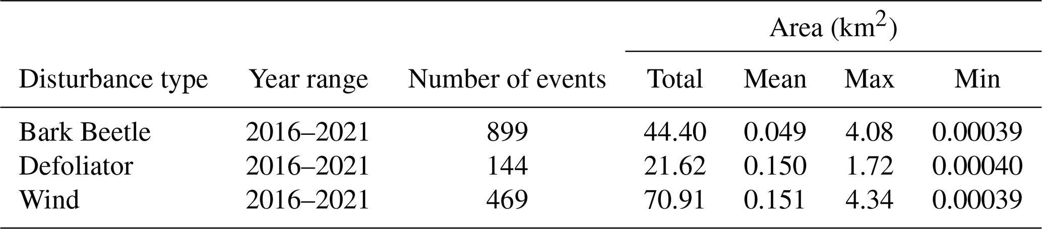
Table 2 summarizes the S1DM disturbance events, showing that bark beetle disturbances are numerous but small in area, defoliator events are fewer but larger on average, and wind disturbances are intermediate in both frequency and size.
Table 2Summary statistics of S1DM disturbance events by type over 2016–2021. The table shows the number of detected events and the total, mean, maximum, and minimum areas (km2) for each disturbance type.
4.1 Spatial and temporal agreement of IDS and radar-based disturbance detection
Specifically, we assessed how many IDS disturbance events contained a corresponding S1DM signal within a 500 m buffer around each IDS patch.
Figures 3 and 4 show that the detection effectiveness of S1DM varies by disturbance type. Wind disturbances have the highest agreement, with 98.4 % of IDS wind events having a corresponding S1DM signal within the 500 m buffer (469 of 478 events). Bark beetle disturbances follow, with 76.3 % of IDS patches matched by S1DM (899 of 1177 events). Agreement is lower for defoliator disturbances, with only 67.8 % of IDS-disturbed areas captured by S1DM (144 of 213 events). The percentages in Fig. 4 refer to totals across all years and match the absolute numbers reported in Fig. 3.
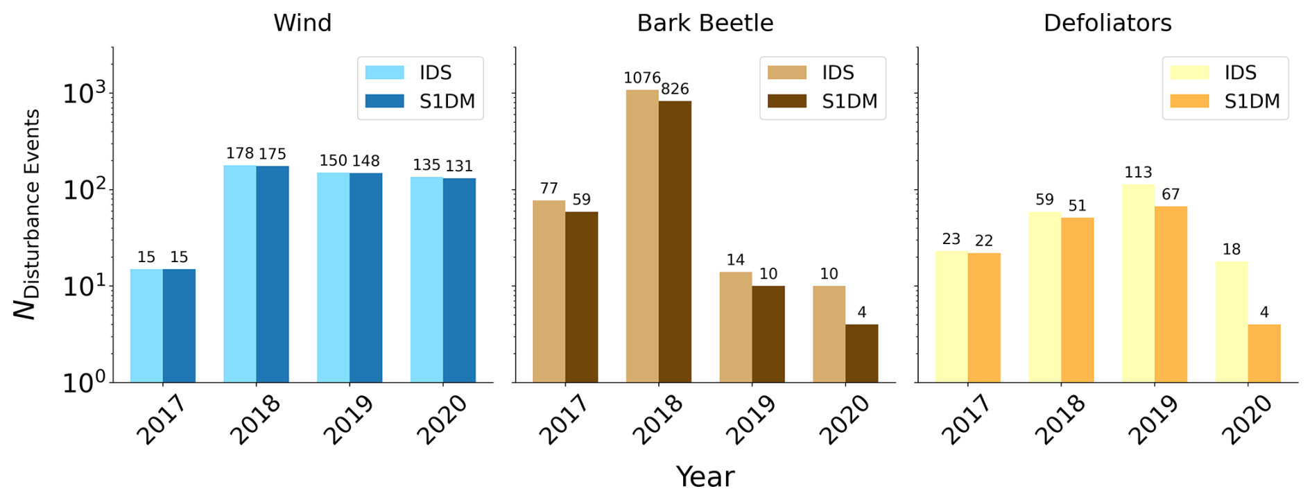
Figure 3Detection efficiency of various disturbance types using Radar Change Detection. The bar plot shows the number of events on the y-axis (log scale) for each disturbance type on the x-axis, with IDS shown in light color and S1DM in darker color. The total number of IDS disturbance events that had a corresponding S1DM signal within the 500 m buffer was 469 for wind (S1DM: 469; IDS: 478), 899 for bark beetles (S1DM: 899; IDS: 1177), and 144 for defoliators (S1DM: 144; IDS: 213).
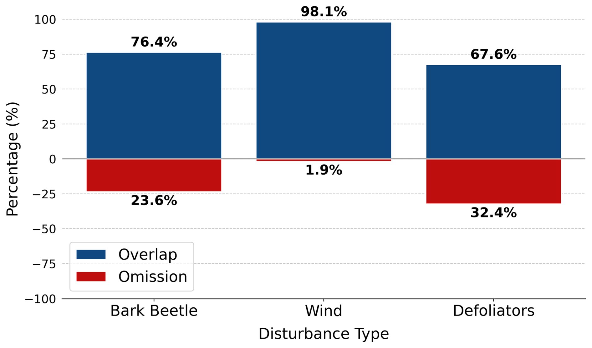
Figure 4Overlap (blue) and omission (red) of IDS disturbance events with Sentinel-1 detections. The x-axis shows disturbance types (bark beetles, wind, defoliators), while the y-axis indicates the percentage of IDS events that were either detected by the Sentinel-1 Change detection or omitted. Blue bars represent IDS events with overlapping Sentinel-1 detections, and red bars show IDS events without a corresponding Sentinel-1 detection (omission).
We analyzed the event size and spatial position of S1DM relative to IDS (without buffer). To quantify this relationship, we examine the spatial agreement between IDS and S1DM for each disturbance type (Fig. 5) by calculating (a) the percentage of IDS polygons covered by S1DM and (b) the percentage of S1DM polygons that overlap with IDS. When examining the overlap without a buffer, we find that IDS is covered to a limited extent by S1DM polygons, with median coverage across all disturbance types remaining below 10 %. There is no overlap for most bark beetle events, and for all other disturbance types, IDS is covered by less than 16 % of S1DM polygons in 50 % of the cases. When examining S1DM polygons, the proportion of each polygon's area that overlaps with IDS is generally low for bark beetle and defoliator events. Only for wind disturbances is the median overlap higher, with more than half of the S1DM polygons showing substantial IDS coverage, indicating better agreement between the datasets for this disturbance type.
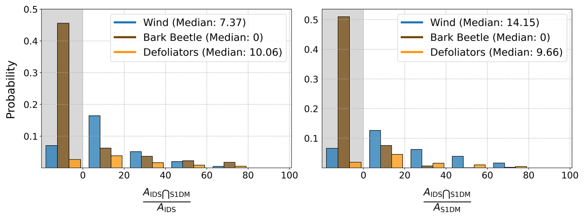
Figure 5Probability of (a) IDS polygons being covered by S1DM, and (b) S1DM polygons overlapping with IDS, for each disturbance type. Disturbance types are color-coded as follows: wind (blue), bark beetles (brown), and defoliators (yellow). Median probabilities for each disturbance type are indicated in parentheses in the legend.
To explore whether overlap differences arise from variations in polygon sizes, spatial spread, or spatial offsets between IDS and S1DM events, we analyzed these three spatial properties (calculated in Sect. 3.3) for the disturbance events in IDS and S1DM, as shown in Fig. 6 and Table 3.
Table 3Summary of disturbance area and centroid shift metrics for IDS and S1DM datasets. The table compares the median (50 %) and 90th percentile of detected disturbance areas (AD) and convex hulls (ACH), as well as centroid shift (ΔCentroid) between datasets.
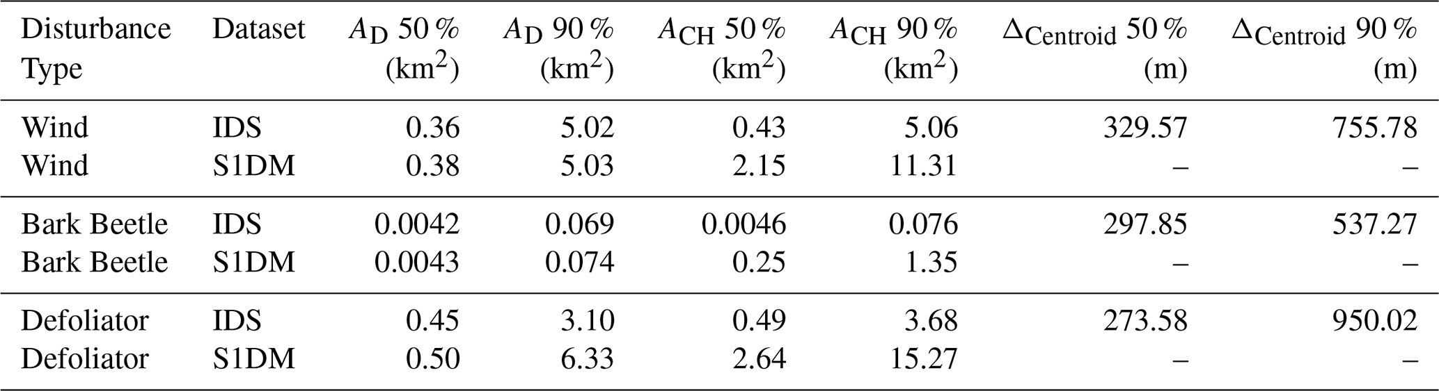
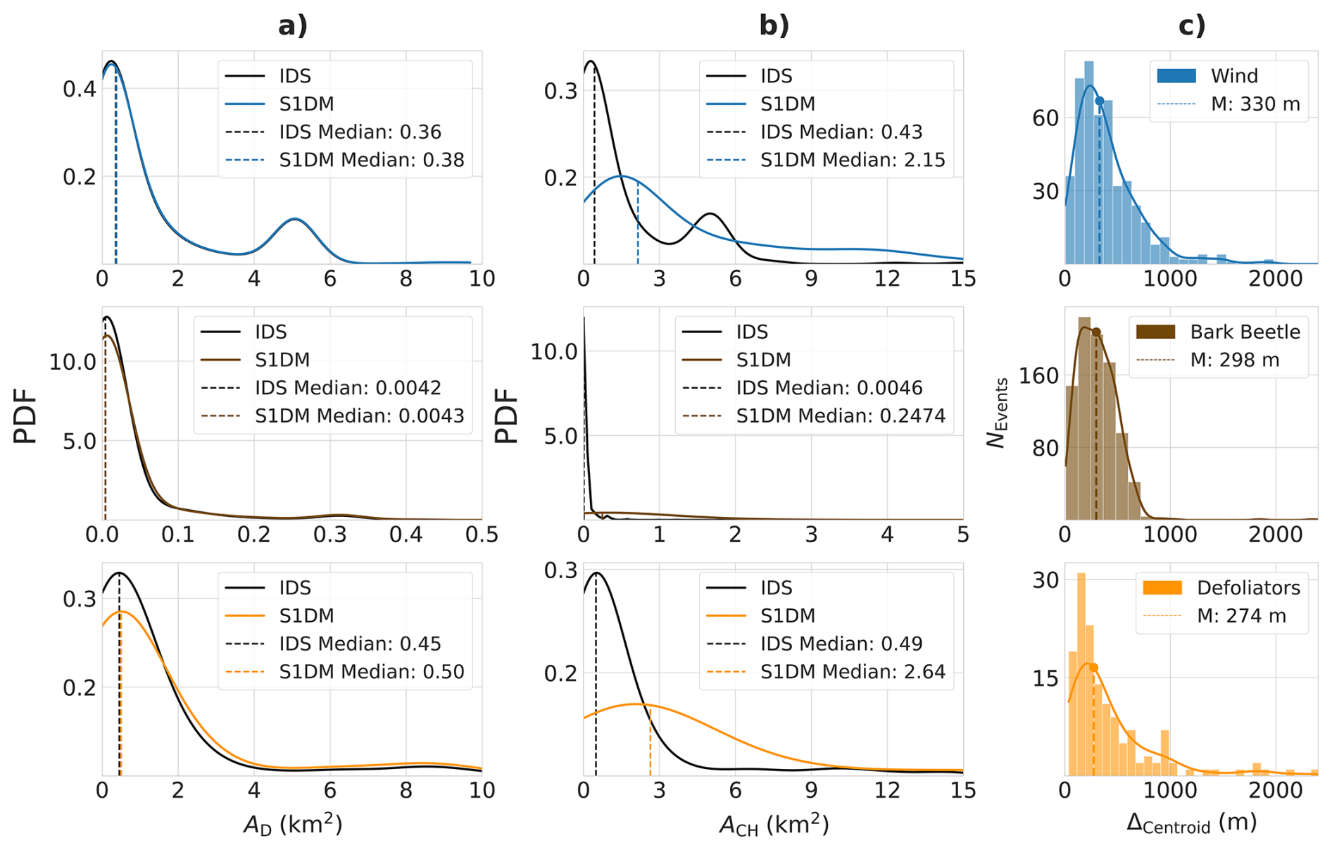
Figure 6Comparison of disturbance size (in km2) and spatial bias (in m) between the IDS and S1DM datasets. The figure consists of three vertical panels, each displaying the results for three disturbance types: wind (top, blue), bark beetles (second, brown), and defoliators (third, green). (a) shows the probability density function (PDF) of disturbance patch areas for IDS (black lines) and S1DM (colored lines) across the four disturbance types. (b) presents the PDF of the convex-hull (CH) areas, representing the spatial spread of the disturbance polygons, using the same color scheme for S1DM and IDS as in the left panel. (c) displays histograms and corresponding PDFs of the spatial distance between IDS and S1DM centroids for each disturbance type.
Our findings reveal no notable differences in the individual size of disturbances across different types of events (Fig. 6a). We find that wind disturbances tend to be the largest events, with 50 % of events having a size of 0.36 km2 or smaller (90 % smaller than 5.02 km2), followed by defoliators with a median area of 0.45 km2 (90 % below 3.10 km2) and bark beetles with the smallest patches, with a median value of 0.0042 km2 (90 % smaller than 0.07 km2).
Overall, disturbance areas derived from S1DM closely match those from IDS, with only minor differences across disturbance types. Bark beetle disturbances show the strongest agreement, with nearly identical median areas (IDS: 0.0042 km2; S1DM: 0.0043 km2) and 90 % of events in both datasets smaller than 0.08 km2. For wind disturbances, median S1DM events are slightly larger than IDS (0.38 vs. 0.36 km2), while the 90th percentile areas are nearly identical (5.02 vs. 5.03 km2). Figure 6a shows a pronounced peak in the probability density function at approximately 4–6 km2 for wind-related disturbances, which is consistently observed in both the IDS and S1DM datasets. Defoliator disturbances tend to be larger in S1DM than in IDS, with similar median values (0.50 vs. 0.45 km2) but substantially larger upper-tail events, where the 90th percentile in S1DM is nearly twice that of IDS (6.33 vs. 3.10 km2).
Figure 6b illustrates the area of the convex hulls enclosing the IDS and S1DM polygons, which serves as an indicator of how spatially dispersed each disturbance event is. In the IDS dataset (without buffer), each event is represented by a single, compact polygon. In contrast, the corresponding S1DM event may consist of multiple scattered polygons (a multipolygon) that encompass all S1CD patches within the 500 m buffer used during S1DM generation. This results in spatially fragmented event structures, as shown in Fig. A1. Accordingly, Fig. 6b demonstrates that S1DM events exhibit a substantially larger spatial extent than the corresponding IDS polygons across all disturbance types. These ratios, reflecting the relative spatial spread of S1DM to IDS, are also summarized and calculated from the values in Table 3. The median convex hull area of S1DM polygons is 5.3 times greater for defoliators (0.49 (IDS) → 2.64 (S1DM) km2) and 5 times greater for wind (0.43 → 2.15 km2) than for the respective IDS polygons. At the 90th percentile, these differences narrow, with the S1DM spread being 4.1 times larger for defoliators (3.68 → 15.27 km2) and 2.2 times larger for wind (5.06 → 11.31 km2). Bark beetle disturbances show the most pronounced increase, with the convex hull area more than 50 times larger for 50 % of events (0.0046 → 0.25 km2) and 17.8 times larger for 90 % of events (0.076 → 1.35 km2), although their overall affected area remains comparatively small, as discussed in Fig. 6a.
We further analyze the spatial bias between the centers of IDS and S1DM disturbance events (Fig. 6c). Despite the pronounced differences in spatial extent and fragmentation, the centroids of corresponding events in both datasets remain closely aligned. Most S1DM centroids fall within 200–350 m of their respective IDS polygon centroids, indicating a strong spatial correspondence between mapped disturbance locations. Even at the 90th percentile, centroid distances remain below 1 km for the majority of events, suggesting that while S1DM polygons are more spatially dispersed, their overall positioning relative to IDS remains consistent.
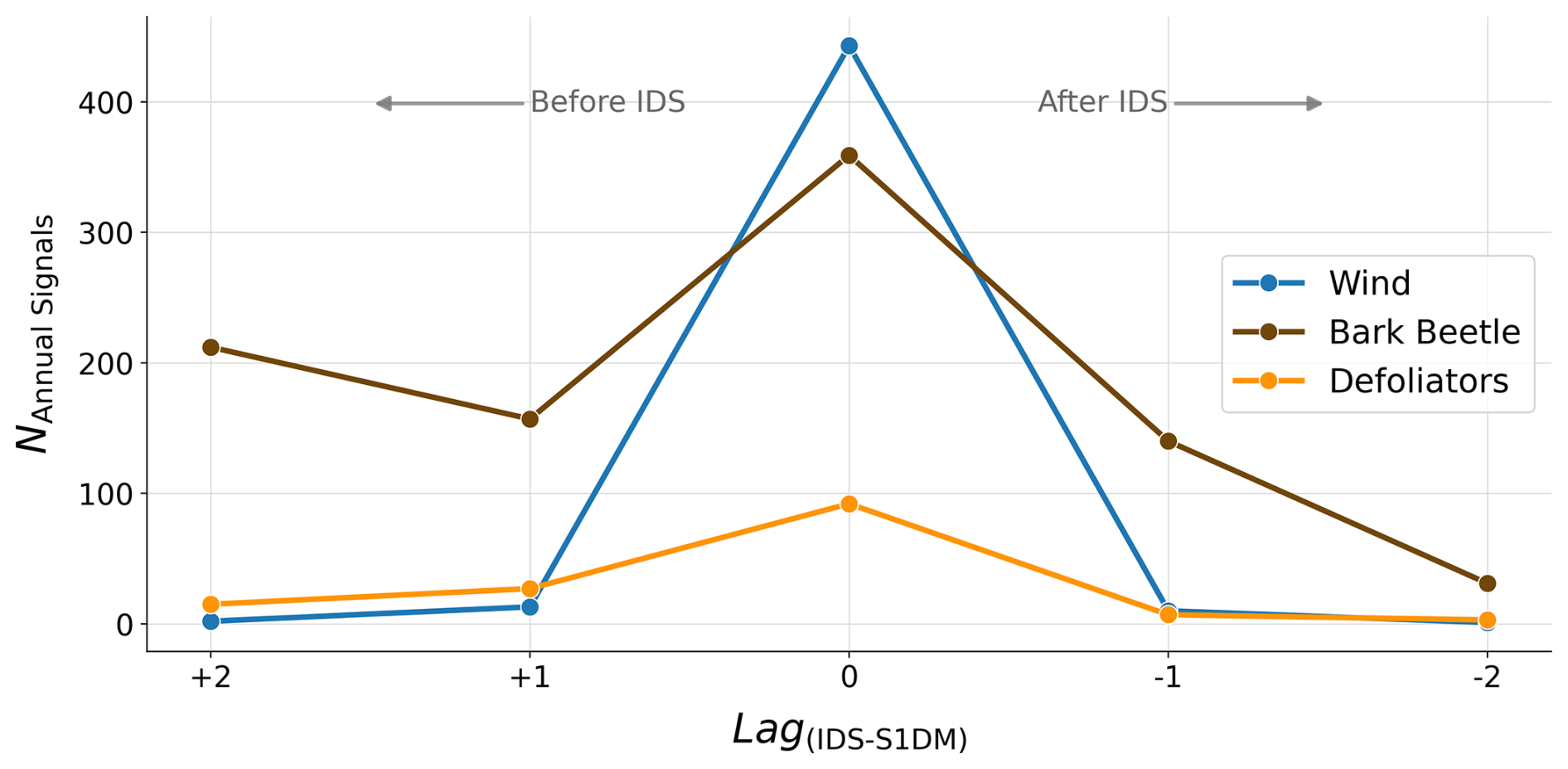
Figure 7Temporal relationship between disturbance detection by S1DM and IDS. The x-axis represents the temporal yearly agreement with IDS – S1DM. The y-axis shows the count of events corresponding to each year's lag, with different disturbance types represented by distinct colored lines. We focus on the single S1DM timestamp closest to the IDS year for each event. We calculate the temporal lag by subtracting the S1DM detection year from the IDS year. Negative values indicate that S1DM detection occurred after IDS, while positive values indicate earlier radar detection.
We analyzed the temporal agreement between corresponding events in IDS and S1DM (Fig. 7). We assess the temporal agreement between the datasets by identifying, for each IDS event, the S1DM detection year that is closest in time. This allows us to quantify how many of the S1DM-detected disturbances correctly coincide in time with those reported by IDS. Overall, S1DM accurately captures the timing of most disturbance events, as reflected by the high number of events detected at a temporal lag of zero (Lag =0) across all disturbance types. Specifically, for wind disturbances, 443 out of 469 S1DM events (94.5 %) occur in the same year as the corresponding IDS events, indicating excellent temporal agreement. For defoliators, 92 out of 144 S1DM detections (63.9 %) coincide with the IDS year (Lag =0), demonstrating moderate agreement but a clear temporal correspondence between the two datasets. Both wind and defoliator events exhibit only limited temporal mismatch, with detections outside the IDS year (Lag or ±2) accounting for less than 3 % of wind and 29 % of defoliator events, respectively. This indicates that, for these disturbance types, S1DM tends to identify a disturbance within the correct year. In contrast, bark beetle disturbances display a broader temporal distribution. While the largest proportion of events, 359 out of 899 (39.9 %), are detected by S1DM in the same year as IDS (Lag =0), a substantial number fall within the ±1-year window around the IDS detection year, with 140 events (15.6 %) detected one year earlier and 157 events (17.5 %) one year later. Notably, 212 events (23.6 %) are detected by S1DM approximately two years earlier than IDS, representing the second-largest peak after Lag =0. This pattern suggests that bark beetle disturbances may be identified earlier in radar-based data, potentially capturing the onset of canopy-structure changes before visible defoliation is recorded in IDS.
The temporal agreement of the S1CD signal should, however, be interpreted cautiously, as we find prolonged signals within the ±2-year time window used for the trend-break detection Fig. A2. For example, due to the detection algorithm, it is possible for a wind event to be detected over multiple consecutive years, although such events are in fact abrupt. Furthermore, temporally continuous signals may reflect other changes, such as clear-cutting or post-disturbance restoration activities. This issue will be further explored in Sect. 5.
4.2 Assessment of spatial patterns in disturbed patches
Since both the S1DM and the IDS datasets exhibit spatial and temporal uncertainties (see Sect. 2.2), we assessed their temporal and spatial accuracy against a set of 15 manually labeled events per disturbance type, derived from PlanetScope images (see Methods). Figure 8 illustrates three representative disturbance events for wind (first row), bark beetles (second row), and defoliators (third row), where the polygons of our manual labels, IDS and S1DM, are overlayed on the RGB composite of the first image showing a disturbance event in that location. For these examples, S1DM appears to capture the spatial extent of disturbances more accurately than IDS. For example, for defoliator and bark beetle events, IDS identifies a smaller area than the RGB composite indicates, whereas for wind disturbances, both IDS and S1DM appear to identify disturbed areas that are not evident in the RGB composite (and thus our manually defined polygon). Overall, the S1DM polygons also appear to show more patchy and irregular spatial outlines compared to both manual and IDS polygons, reflecting the finer resolution and method used for their generation.
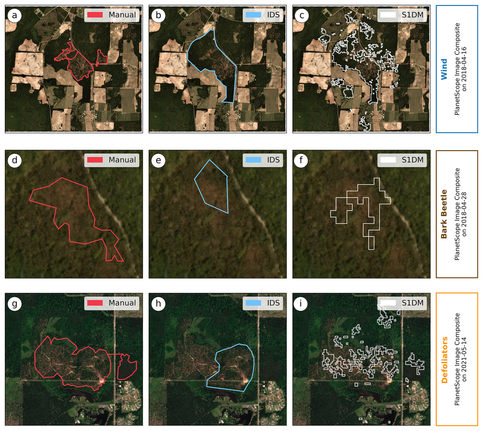
Figure 8Spatial analysis of forest disturbance datasets using PlanetScope (3 m) imagery, illustrating different labeling approaches: manual delineation (red), IDS (blue), and S1DM (white). Images are arranged row-wise by disturbance type (wind, defoliators, bark beetles) and displayed over the corresponding PlanetScope scene composites. In the first column (a, d, g), the manually delineated polygons using PlanetScope imagery are shown. The second column (b, e, h) shows the corresponding IDS polygons in light blue, while the third column (c, f, i) presents the S1DM polygons in white.
In Fig. 9, we quantify the spatial agreement of IDS and S1DM polygons with the 3 × 15 manually labeled polygons from PlanetScope imagery, using both percentage overlap and the Intersection over Union (see Methods Sect. 3.5). S1DM polygons show substantially higher agreement with manual labels than IDS for wind and bark beetle disturbances, with median values (see Table A6) of IoU (panel (a)) of 0.157 and 0.076 for wind and bark beetle events detected by S1DM, respectively, compared to 0.092 and 0.007 for IDS. For the spatial overlap, S1DM estimates a median value of 44.3 %, 20.1 %, and 22.2 % for wind, bark beetles and defoliators, compared to 12.3 %, 0.7 %, and 22.7 % for IDS.
One-sided Wilcoxon rank tests indicate that the improvement in the spatial agreement is significant for both wind and bark beetles with both metrics, although for wind only at 90 % significance for the Intersection over Union. No statistically significant improvement is observed for defoliator disturbances according to the one-sided Wilcoxon rank test. It is worth noting that the Intersection over Union remains generally low, consistently below 0.4, while the percentage overlap ranges from 0 % to 60 %. This might be due to uncertainties in both S1DM and IDS, as well as to the visual labeling approach that relies on the RGB signal.
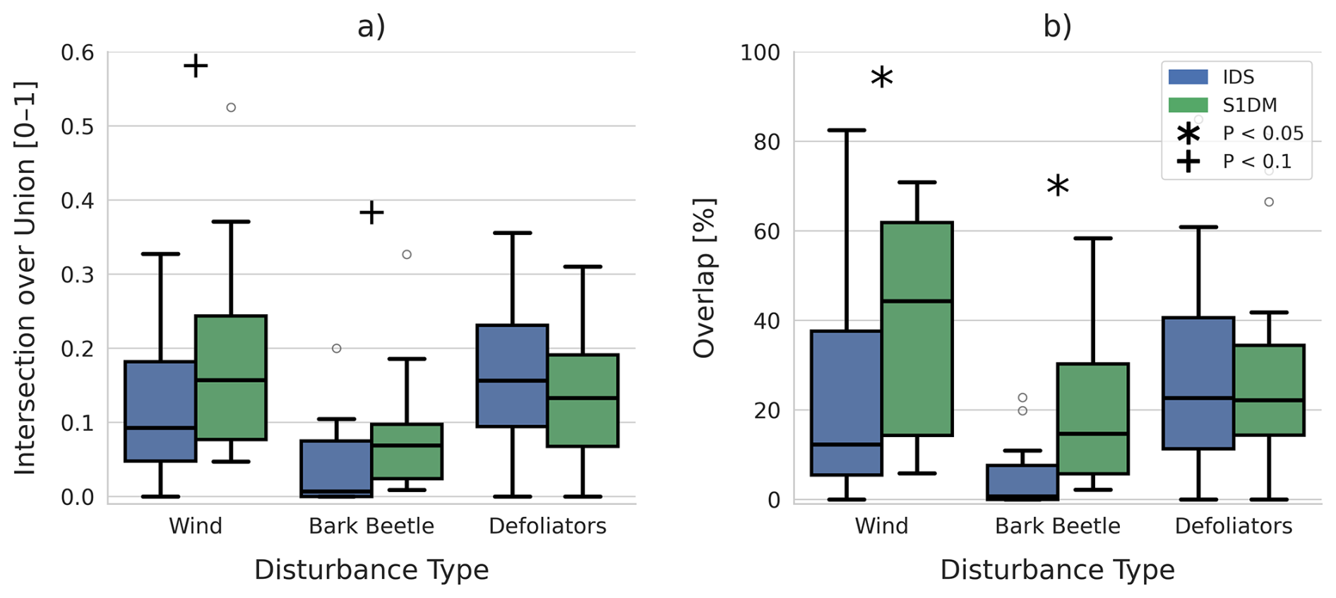
Figure 9Comparison of agreement between IDS and S1DM disturbance maps with manually delineated reference polygons. Panel (a) shows the Intersection over Union, and panel (b) shows area overlap (in percentage), both displayed as box plots. Statistical significance from a one-sided Wilcoxon rank test is indicated by a black star for p<0.05 and a black cross for p<0.1.
We aimed to improve forest disturbance mapping by combining IDS inventory data with Sentinel-1 radar change detection, leveraging IDS’s detailed disturbance-agent information while reducing uncertainty in disturbance size, location, and timing. We find that integrating radar data substantially improves the spatial and temporal characterization of disturbance events, particularly for bark beetle outbreaks and wind damage. The resulting dataset captures both the location and timing of disturbances more accurately than IDS alone. These improvements provide a robust foundation for applications such as training data-intensive, data-driven models for disturbance classification.
5.1 Capabilities and Limitations of Sentinel-1 Change Detection to Improve Forest Disturbance Monitoring
Here, we produced new forest disturbance maps for the southeastern USA covering the period 2016–2021 based on the Sentinel-1 radar backscatter trend detection algorithm by Cremer et al. (2020), S1CD. This algorithm enhanced forest disturbance monitoring by leveraging Sentinel-1's frequent, consistent, and cloud-penetrating radar data to detect significant structural changes in forests. S1CD effectively identified disturbances associated with structural damage, such as bark beetle infestations and storms. As shown in Fig. 3, S1CD successfully detected over 75 % of IDS-recorded wind and bark beetle disturbances in the study region and selected period. However, detection rates dropped significantly for more subtle disturbances, such as those caused by defoliators, with only 67 % of disturbances reported by IDS identified by S1CD.
This limitation is consistent with known challenges in remote sensing of forest disturbances, where gradual or low-intensity disturbances often remain undetected (McDowell et al., 2015). In this case, the low sensitivity of S1CD to subtle and slow-onset disturbances may stem from the change detection threshold, which we set at −1.28 based on the method described in Cremer et al. (2020) and correspondence with the authors. Since the method was optimized to detect abrupt, permanent structural changes, disturbances that unfold gradually or cause only minor canopy loss are likely to have gone undetected. Although lowering the threshold could improve the sensitivity to these subtle disturbances, it would risk increasing noise, leading to more false positives and reducing the detection reliability. Thus, while the Sentinel-1 Change Detection method applied here was highly effective in capturing severe disturbances such as wind-throw and bark beetle outbreaks, its limitations in detecting milder, gradual, or recovering disturbances must be acknowledged.
Additionally, in our IDS preprocessing, we excluded all temporally compound events to retrieve a clear disturbance signal for each disturbance agent. However, by excluding such events, we introduced bias into the dataset, so that our hybrid S1–IDS dataset (S1DM) should not be considered for exhaustive characterization of disturbance occurrence in the study region. While not representative of all disturbance events, the dataset provides a set of “noise-free” disturbance events for each of the three agents considered, which should allow for better training of unsupervised classification models. Below, we discuss the improvements introduced by our hybrid dataset.
5.1.1 Location and delineation of disturbance patches
Previous studies (Backsen and Howell, 2013; McConnell, 2000) noted the challenges in accurately mapping disturbances using aerial surveys, mainly due to the high speeds at which these surveys are conducted. Aircraft speeds of 144–200 km h−1 (100 mph) and altitudes ranging from 305 to 762 m above the canopy make the accurate delineation of disturbance patches difficult (Coleman et al., 2018). To address this limitation, we applied a 500 m buffer around disturbance locations, as determined in the Methods Sect. 3.4 to be an optimal trade-off between retaining relevant events and minimizing noise. The results, shown in Fig. 6c) and Table 3, indicated that 50 % of S1DM disturbance centers fall within 200–355 m of IDS centroids, with most events within 950 m. This suggests that the centers of disturbance patches in both datasets are generally well aligned, given the inherent uncertainty of aerial detection surveys.
The peak at approximately 5 km2 for wind disturbances reflects a combination of genuine large-scale wind damage and methodological artifacts in the IDS data. In 2020, several major tropical cyclones (including Cristobal, Marco, Laura, Delta, and Zeta) affected the region between Houston and New Orleans, producing extensive areas of wind-disturbed forests. In addition, aerial survey procedures were modified due to COVID-19 restrictions, leading to the use of alternative mapping approaches. This resulted in more uniform, often square-shaped disturbance polygons of similar size, particularly in this region, which contributes to the observed peak. Despite this artifact, the mapped polygons still capture the spatial footprint of severe wind-induced forest disturbances.
Our results align with studies showing limitations to the accuracy of aerial surveys, particularly their tendency to overestimate disturbance areas and include healthy, unaffected trees (Hall et al., 2016; Kautz, 2014). We found that the total disturbed area was generally consistent between the two datasets. For 50 % of disturbance events, the size difference was less than 0.2 km2 (Fig. 6a). However, spatial discrepancies remain important. Specifically, Fig. 5 shows that, on average, less than 10 % of the area of IDS disturbance polygons overlaps with S1DM polygons. Similarly, less than 15 % of an S1DM polygon's area is covered by its corresponding IDS polygon, highlighting substantial differences in the spatial distribution of disturbances between the two datasets.
The limited spatial overlap between IDS and S1DM disturbance patches arises from several factors. IDS polygons tend to be large, single polygons, whereas S1DM polygons are often multipolygons, with gaps and holes, resulting in only partial spatial correspondence (Fig. 8). In addition, IDS patches, particularly for wind and defoliator events, often exhibit artificial geometric shapes such as rectangles or squares. These shapes are atypical for natural disturbances and may include healthy, unaffected trees within the polygons (Hall et al., 2016; Kautz et al., 2017; Kautz, 2014). In contrast, S1DM identifies smaller, more irregular patches that better reflect the natural variation of disturbance processes.
S1DM disturbances are frequently distributed around IDS polygons, forming multiple discrete patches that aggregate to a similar total area but with minimal spatial overlap (Fig. 8b, c, and e, f). Slight misalignments or offsets between IDS and S1DM patches further reduce overlap, even when the disturbance sizes are similar (Fig. 8b, d). This pattern is supported by the analyses in Fig. 6 and Table 3, which indicate that S1DM disturbances often cover a wider area compared to IDS.
However, Fig. 8 also illustrates that S1DM can sometimes miss patches entirely, as exemplified in panel i, while in other cases it aligns well with IDS patches (panels b–c). This is primarily due to the threshold applied during Sentinel-1 change detection, where some polygons may not meet the disturbance criteria or fall below the detection threshold.
Our quantitative analysis (Fig. 9) further supports these observations. Randomly sampled elements indicate that wind and bark beetle events are captured more consistently by S1DM than by IDS and align more closely with manual assessments. Only defoliator events show no significant improvement relative to IDS. This highlights both the strengths of S1DM in representing disturbance processes more realistically and its limitations, where the detection threshold can lead to missed events.
Importantly, our analysis underscores that IDS and S1DM can complement each other. While IDS offers a broad, initial assessment, S1DM excels at delineating disturbance patches in greater detail and detecting patches that may be missed due to spatial misalignments or IDS's limited ability to capture the full extent of disturbances. This advantage of S1DM is particularly evident for wind and bark beetle disturbances, where it provides clearer and more realistic patch delineations. However, for defoliator events, S1DM does not show the same improvement over IDS. Therefore, we are confident that our hybrid dataset, S1DM, can provide an improved reference dataset for disturbed areas, facilitating the development of remote-sensing-based classification models.
5.1.2 Timing of disturbances
Accurately assigning the timing of a given disturbance event is generally challenging. Both IDS and S1DM are subject to inherent temporal uncertainties due to their acquisition methods and characteristics. For IDS, temporal uncertainties stem from the nature of aerial surveys. Flights do not always happen at optimal times due to weather, logistics, or survey schedules, leading to disturbances being recorded late or at suboptimal times (McConnell, 2000). This issue is particularly pronounced for biotic disturbances, such as defoliators and bark beetles. Defoliators must be mapped while actively feeding; if surveyors fly too early or too late, the disturbance may be underestimated or missed entirely. Similarly, bark beetle outbreaks often go undetected until tree mortality becomes widespread, creating a delay between the initial attack and recorded detection (Kautz, 2014). Recent work by (Eifler et al., 2026) estimated an average delay of one year between IDS and plot-scale forest inventory information.
Given that IDS already has an average temporal misalignment of over a year, we applied a two-year buffer when comparing IDS and S1DM to ensure a more realistic temporal intersection. Figure 7 illustrates the challenge of precisely pinpointing the timing of the disturbance. The left panel shows that S1DM detected change signals for all disturbance types in the years surrounding the IDS disturbance year. Still, the right panel focuses on the S1DM signal that aligns most closely in time with the IDS disturbance year for each event.
For those events in which S1DM detects a disturbance earlier than IDS, the event likely began the year before it was detected by aerial surveys, indicating potentially a better ability of S1DM for early detection of the onset of disturbance. However, we cannot exclude artifacts resulting from S1DM’s built-in ±0.5-year temporal buffer for trend detection that can cause some disturbances to be attributed to the wrong year. The uncertainty due to the temporal buffer in S1DM could also explain the later detection compared to IDS. However, it could also have a physical cause, especially for events in which human-driven post-disturbance actions, such as salvage logging or clear-cutting, result in more pronounced changes in forest structure that are better captured by the trend detection algorithm.
Biotic disturbances further complicate this, as insect outbreaks can persist for multiple years. Recurring defoliation attacks, for instance, can result in consecutive-year detections that do not necessarily indicate misattribution but rather repeated disturbances. While we excluded disturbed patches that temporally and spatially overlapped in IDS, we cannot exclude the detection of such compound events in S1DM in their close vicinity. Similarly, changes in signals after post-disturbance years in fire and wind events may reflect salvage logging rather than ongoing disturbance.
Disturbance events occur within a complex ecosystem influenced by multiple factors. Gradual mortality, delayed detection, and human-driven post-disturbance actions (e.g., salvage logging or clear-cutting) further complicate the precise determination of disturbance timing. Because we cannot fully disentangle these complexities, we considered the IDS survey year as the reference for further analysis. Figure 7 shows that for most disturbance events, at least part of the detected disturbance was assigned the same year as the IDS survey. However, a notable exception is the number of bark beetle events detected two years before IDS.
5.2 Alternative to Manual Labeling Practices
In addition to providing an improved hybrid forest disturbance reference dataset for disturbance agent classification, our approach aimed to move beyond the traditional, labor-intensive method of manual labeling. The Sentinel-1 Change Detection (S1CD) algorithm enables analysts to bypass the time-consuming task of manually refining disturbance locations, outlines, and timing by using high-resolution radar-based information on forest structure and change. By employing the trend-break detection method of Cremer et al. (2020), we successfully automated much of the re-labeling process, creating an efficient and scalable system that requires a smaller contribution from expert knowledge. This not only reduces the need for manual inspection but also offers a viable alternative to manual labor, minimizing reliance on private, sometimes exploitative labor platforms located in developing countries, as is often the case for deep learning label generation (Aloisi, 2016; Hawkins and Mittelstadt, 2023).
Our semi-automatic labeling method was initially developed to address specific challenges in reference dataset quality (see Sect. 1). A key advantage of our semi-automated labeling method is its adaptability to different regions, as long as some form of inventory-based disturbance data, e.g., the Canadian Forest Service’s National Forestry Database (NFD), the Database of Forest Disturbances in Europe (Patacca et al., 2021, DFDE), the Dataset of wind Disturbances in European Forests (Forzieri et al., 2020, FORWIND), or the Database of European Forest Insect and Disease Disturbances (Forzieri et al., 2023, DEFID2), is available. Sentinel-1 data, available globally since 2014, provides a consistent and uninterrupted record of forest dynamics. Unlike optical datasets, such as Sentinel-2, which are susceptible to cloud cover and atmospheric interference, Sentinel-1’s radar data enable reliable time-series analysis across diverse climatic conditions. This robustness makes it particularly valuable for monitoring large-scale and long-term disturbances.
However, Sentinel-1 data is affected by terrain-induced distortions in mountainous regions, which can reduce classification accuracy (Small, 2011; Imperatore, 2021). Users should exercise caution when applying this method in areas with significant elevation changes, as radar signal distortions can impact data reliability. Despite this limitation, our approach remains broadly applicable, especially in flat or gently sloping landscapes, where radar performance is more stable.
5.3 Methodological Assumptions and Limitations
In this study, several methodological decisions had to be made that could potentially influence our results. To combine disturbance information from IDS and S1CD, we used a spatial buffer of 500 m and a temporal buffer of ±2 years centered on the IDS disturbance date. This spatial and temporal buffer was introduced to account for the spatial and temporal uncertainty in both the IDS dataset Eifler et al. (2026) as well as in the disturbance date detection by S1CD.
Previous work by Eifler et al. (2026) analyzed the spatial and temporal agreement in reported disturbances for IDS and the Forest Inventory and Analysis (Woudenberg et al., 2010) for the continental U.S. An analysis of spatial buffers of 800 and 1600 m, showed that increasing buffer size introduced additional uncertainty. The disturbance timing differed by 0.7 years on average, for a buffer size of 800 m. We have tested the effect of using different spatial buffer sizes of 100, 250, 500, and 1000 m on the number of events retained for analysis, and found that buffer sizes of 100–250 m resulted in too few events being selected, while 1000 m did not retain considerably more events. Furthermore, our change detection algorithm is based on recurrence analysis trends over 2-year-long windows, meaning that the difference in the timing of disturbance with IDS could be up to 2 years, if the disturbance happened at the end of the analysis period. Therefore, our choice of 500 m and 2-year windows represents a balance between retaining information and minimizing the risk of introducing additional uncertainties. Future work could explore in greater detail the impact of spatial uncertainty between inventory datasets and satellite observations to refine buffer selection.
Another key methodological limitation concerns the selection of the temporal threshold for classifying structural changes. Like most other disturbance detection approaches (van der Woude et al., 2026; Hirschmugl et al., 2017; Kennedy et al., 2010), our algorithm requires a change in the temporal structure of the VH signal that is sharp enough to be distinguished from normal variability. In this study, we applied a threshold of −1.28 of the RQA-TREND calculated over a 2-year window centered around each year's summer to distinguish between stable and disturbed pixels. While this value was empirically derived from reference datasets, it remains a heuristic choice and can influence the spatial coherence and apparent patchiness of detected disturbances. We tested the effect of this choice by evaluating the performance of the S1CD in detecting the set of manually labeled disturbance patches from PlanetScope for different values of the RQA-TREND and per disturbance type (Fig. A3). The results indicate that the optimal thresholds differ among disturbance agents, with wind and Bark-beetle requiring sharp changes in the temporal structure of the SAR signal, while defoliators are better captured if less strict thresholds are used. The selected threshold of −1.28 falls within the broader range of optimal values across disturbance types and metrics, representing a compromise solution that ensures consistent applicability across all disturbance categories. We explicitly acknowledge this dependency as a limitation of our workflow. The analysis highlights that, in principle, a universal “one-size-fits-all” change-detection threshold does not exist. These results are consistent with and underscore the challenges in monitoring from space disturbance with very different spatial and temporal characteristics, as discussed, e.g., by McDowell et al. (2015). We therefore recommend adopting disturbance-specific threshold calibration strategies, as global fixed thresholds are known to produce biased results across ecosystems and disturbance types due to differences in vegetation structure, disturbance dynamics, and sensor response (McDowell et al., 2015; Cohen et al., 2010; Verbesselt et al., 2010; Zhu and Woodcock, 2014; Senf and Seidl, 2018).
A key limitation in disturbance detection workflows is the propagation of errors through sequential processing steps; for example, a misclassification in one dataset can influence the final combined disturbance map. Our framework is explicitly designed to reduce error propagation by integrating multiple sources of disturbance information, including Sentinel-1 change detection. While direct field validation would provide the strongest confirmation of disturbances, this is not possible in our case: the events we analyze occurred 5–9 years ago over a very large region, and many affected areas have likely recovered (for example, defoliator impacts often recover within a year). Previous work has explicitly assessed inconsistencies and uncertainties in IDS. Eifler et al. (2026) compared IDS with independent inventory data and found good temporal agreement with FIA, suggesting that temporal errors in IDS are generally low. Our results support this finding, as IDS timing largely aligns with S1DM (Fig. 7), except that some bark beetle disturbances are detected earlier by S1DM than reported in IDS. However, because FIA lacks sufficiently detailed spatial information, spatial event-level errors cannot be quantified using inventory data alone. To address this limitation, we employed Planet imagery as an independent, spatially explicit proxy for validation. Although this cannot fully replace field observations, it allows us to evaluate the plausibility of disturbances in areas where ground data are no longer available.
In this study, our analysis was constrained to areas covered by the IDS dataset, which provides detailed, spatially explicit information on disturbance agents. While Sentinel-1 offers global coverage and the potential to detect disturbances beyond regions surveyed by aerial or ground-based inventories, the lack of independent reference data limits our ability to confidently attribute detected disturbances to specific causal agents in areas outside IDS coverage. Consequently, the current framework cannot fully evaluate the performance of Sentinel-1-based disturbance detection across unsurveyed regions or in landscapes where IDS data are absent. Future work should address these limitations by integrating Sentinel-1 disturbance detection with high-resolution, independent reference datasets, such as manual delineations from Planet imagery, and by using tree canopy cover products to exclude non-forested areas. Expanding the analysis in this way would allow for a more comprehensive assessment of Sentinel-1’s capabilities and its potential for large-scale, autonomous forest disturbance monitoring.
5.4 Generalizability and applications of the proposed approach
Our study demonstrates that integrating Sentinel-1 spatio-temporal information can help refine disturbance mapping from inventory datasets. The data processing pipeline is provided alongside this study (see GitHub in Code Availability), so that it can be extended to other regions, as well as different combinations of inventory and satellite-based datasets. We discuss some possible applications and considerations regarding the generalizability of this approach below.
The approach proposed here can be easily applied to other inventory datasets and satellite missions, provided they have overlapping spatial and temporal coverage. The structural information inherent in SAR backscatter data and the high spatial resolution of Sentinel-1 offer opportunities to enrich existing forest disturbance inventories, improve temporal and spatial resolution, and reduce uncertainty in forest loss mapping. For IDS, which is already spatially explicit, S1CD improved the spatial delineation of the disturbed patches, especially for bark beetles and wind (Fig. 9). Therefore, our study shows that SAR-based change detection provides a valuable complementary source of information to aerial surveys and field inventories. For point-based inventory datasets, such as National Forest Inventories (Woudenberg et al., 2010), S1CD provides a means to expand the spatial information of the data, provided that precise coordinates are available for forest inventory plots. The pipeline can also be adapted to other existing satellite-based forest disturbance datasets, such as the Global Forest Change (Hansen et al., 2024), or the European Forest Disturbance Atlas (Viana-Soto and Senf, 2025). The main bottleneck for extending the application to other regions remains the limited availability of suitable inventory datasets, i.e., with large-scale spatial and temporal coverage and detailed and consistent forest disturbance agent information, ideally spatially explicit and with precise coordinates, and that are publicly available and that follow FAIR principles (findable, accessible, interoperable, and reusable). However, recent efforts to compile information on specific forest disturbances, (e.g. Forzieri et al., 2020, 2023; Urquiza-Muñoz et al., 2024) might still be useful. With appropriate reference datasets, however, there are no inherent technical limitations that prevent extending the methodology to other regions or larger spatial extents. Therefore, initiatives such as European Union's proposal for a Forest Monitoring Framework (European Commission, 2023), aiming to facilitate access to forest-relevant data, including forest disturbances (Migliavacca et al., 2025) would allow expanding and testing our approach in other regions.
An open question that remains is whether this approach is transferable to regions with complex topography, such as mountainous areas. Our study region is limited to the southeastern United States, which is relatively flat and was selected because of its high incidence of wind disturbances. The absence of large mountains avoids topographic-induced uncertainties known to affect Sentinel-1 observations (Shi et al., 2024; Borlaf-Mena et al., 2020). While the framework performs well under these conditions, its application in more mountainous regions would require additional testing. In addition, differences in forest structure and species composition may require region- or forest-type-specific adjustments to parameters, particularly for backscatter dynamics and disturbance signatures. In this context, other satellite-based information sources could replace, or complement the S1CD mapping, for example, vegetation indices reflecting other canopy properties from spectral imagery (Senf et al., 2015; Senf and Seidl, 2018; Canadell et al., 2021b; Hall et al., 2016), or hyperspectral information from new missions such as ENMAP (Vanguri et al., 2024).
Various forest disturbance classification algorithms have been developed to separate different disturbance types (Schleeweis et al., 2020; Senf and Seidl, 2021b; Senf et al., 2015; Oeser et al., 2017; Helmer et al., 2010; Baumann et al., 2014). The three disturbances considered here, wind, bark beetles, and defoliators, are particularly hard to disentangle, given their particular spatial and temporal characteristics (e.g. McDowell et al., 2015; Schleeweis et al., 2020; Viana-Soto and Senf, 2025). With increasing interest in exploring machine learning (ML) or deep learning (DL) models for forest disturbance classification (Stahl et al., 2023; Kislov et al., 2021; Chen et al., 2021), having large-scale spatially and temporally consistent data on the different disturbance types is key either as training labels for supervised models, or else as evaluation data for new classification models in general. The S1DM dataset addresses this need, in that it contains a subset of IDS-based disturbed patches for these three disturbance types, with refined spatial delineation (Fig. 9) and temporal information, as S1CD tends to detect bark beetle, and to some extent also defoliator, disturbances earlier than they are reported in IDS (Fig. 7). This reduced set of disturbed patches is still large enough (469, 899, and 144 samples for wind, bark beetles, and defoliators, respectively, over a region of 1 701 214.39 km2) to support the development of dedicated and data-intensive classification algorithms to separate these different disturbance types.
In this way, the refined dataset provides a foundation for the development of adaptive classification frameworks that can generalize across regions, forest types, and disturbance regimes.
Reliable, spatially and temporally consistent information on forest disturbances, particularly wind, bark beetles and defoliator insects, remains a major bottleneck for large-scale disturbance attribution and modeling (Kautz et al., 2017; Rodríguez Paulino et al., 2024). In this study, we directly address this limitation by refining the widely used legacy Insect & Disease Survey (IDS) by integrating Sentinel-1-based radar change detection (S1DM). This hybrid approach leverages the complementary strengths of both datasets: the long-term, agent-specific information provided by IDS (Forest Service U.S. Department of Agriculture, 2024) and the spatially and temporally continuous, cloud-independent structural sensitivity of C-band SAR observations.
Our analysis specifically targets three key sources of uncertainty in legacy disturbance inventories: disturbance location, disturbance outline, and disturbance timing (Eifler et al., 2026; Coleman et al., 2018; Andrus et al., 2025). Although S1CD shows reduced sensitivity to subtle canopy changes, such as those associated with defoliator activity, it performs well for structurally significant disturbances, including wind damage and bark beetle outbreaks, a performance consistent with (Bruggisser et al., 2021), that demonstrated that Sentinel-1 can reliably detect decreases in forest height greater than 10 m. Spatially, disturbance centers were generally within 200–950 m of one another. Although the overall disturbed area remained similar, the S1DM dataset identified more physically plausible disturbance patterns, with wind and bark beetles showing significantly improved agreement with independent manual reference data compared to IDS (see Fig. 9).
Improving disturbance mapping enables downstream calculations, such as quantifying actual forest loss, estimating carbon emissions by disturbance type, and correcting uncertainty in carbon loss (Harris et al., 2016). The new hybrid dataset proposed here also addresses key challenges in forest disturbance classification and prediction algorithms, particularly those based on machine- and deep learning models (ML and DL, respectively) (Rodríguez Paulino et al., 2024). These data-intensive methods require large amounts of reliable, agent-specific training data. By reducing spatial and temporal noise in IDS, S1DM provides a publicly available, standardized benchmark dataset for training and validating methods for forest disturbance classification and prediction. Combined with complementary remote sensing products such as Sentinel-2 or Landsat, this approach has the potential to improve disturbance detection and classification, including the differentiation of subtle disturbance types, such as between different insect disturbance agents or between wind and bark beetle compound events. Previous studies have demonstrated that such distinctions are possible at local or site scales for individual events using optical or multi-sensor data (Eklundh et al., 2009; Meddens et al., 2012; Senf et al., 2015; Negrón-Juárez et al., 2018; Senf and Seidl, 2018; Candotti et al., 2022). However, the systematic and large-scale application of these approaches remains challenging due to limited reference data and the complexity of disturbance dynamics. In this context, S1DM provides a resource that supports the development of scalable, automated disturbance classification frameworks and facilitates the study of ecologically relevant disturbance processes across broader spatial and temporal extents.
Despite these advances, some uncertainties remain, particularly regarding the precise timing and duration of gradual disturbances. Future work could explore integrating additional data streams, such as Sentinel-2 time series, and advanced learning strategies to further reconcile information from IDS, S1DM, and optical observations, particularly in cases where neither dataset fully captures the disturbance signal. Overall, our approach offers a scalable and substantially less labor-intensive alternative to manual labeling and is readily transferable to other regions and legacy inventories (FORWIND; Forzieri et al., 2020; DEFID2; Forzieri et al., 2023). By improving the reliability of disturbance reference data, this work lays the groundwork for more robust data-driven analyses of forest disturbance dynamics across large spatial and temporal scales.
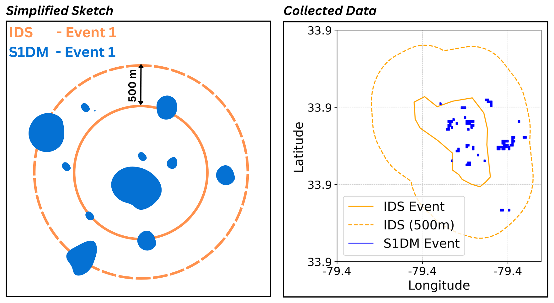
Figure A1Schematic (left) and data-driven (right) representations of the intersection between IDS and S1CD. On the left, a conceptual diagram illustrates how each S1CD polygon intersecting with an IDS event's buffered (500 m) boundary is combined into a multi-polygon, effectively merging multiple S1CD polygons associated with a single IDS event. The right panel illustrates this process applied to real data, where intersecting S1CD polygons are grouped and treated as a single unified event, similar to the treatment of IDS polygons.
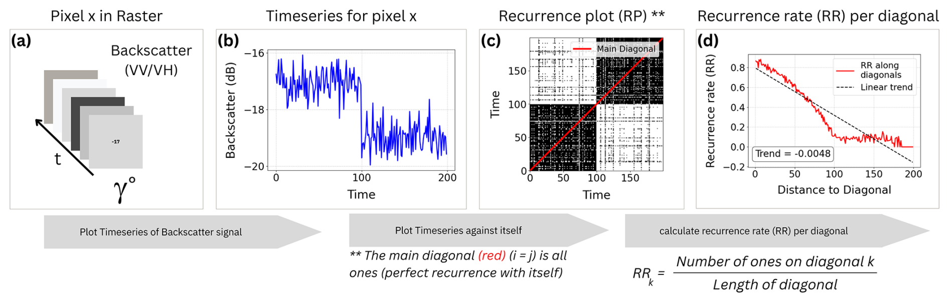
Figure A2Schematic representation of recurrence analysis for a Gamma backscatter pixel. (a) Singular Pixel of one Sentinel-1 Raster Tile (b) Time series of the pixel showing a sudden change (“break”) in backscatter values. (c) Recurrence plot (RP) highlighting times when the signal revisits similar states; the main diagonal is shown in red. (d) Recurrence rate (RRi) computed along off-diagonals of the RP, with a linear trend (dashed line) indicating the rate of drift in the system. The slope of the trend quantifies whether the process is stationary or drifting over time.
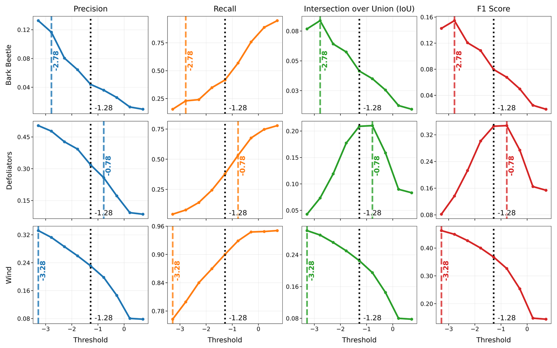
Figure A3Comparison of classification metrics across thresholds for each disturbance agent (DCA_ID). For each metric – Precision, Recall, Intersection over Union, and F1 Score – the curves show the metric values as a function of the applied threshold. Vertical colored dashed lines indicate the “best threshold” that maximizes F1 for each DCA_ID, while the dotted black line marks the fixed medium threshold of −1.28 used across all agents in this study. The figure illustrates the variation in optimal thresholds between disturbance types and highlights the compromise inherent in selecting a universal threshold for consistent application across multiple disturbance agents.
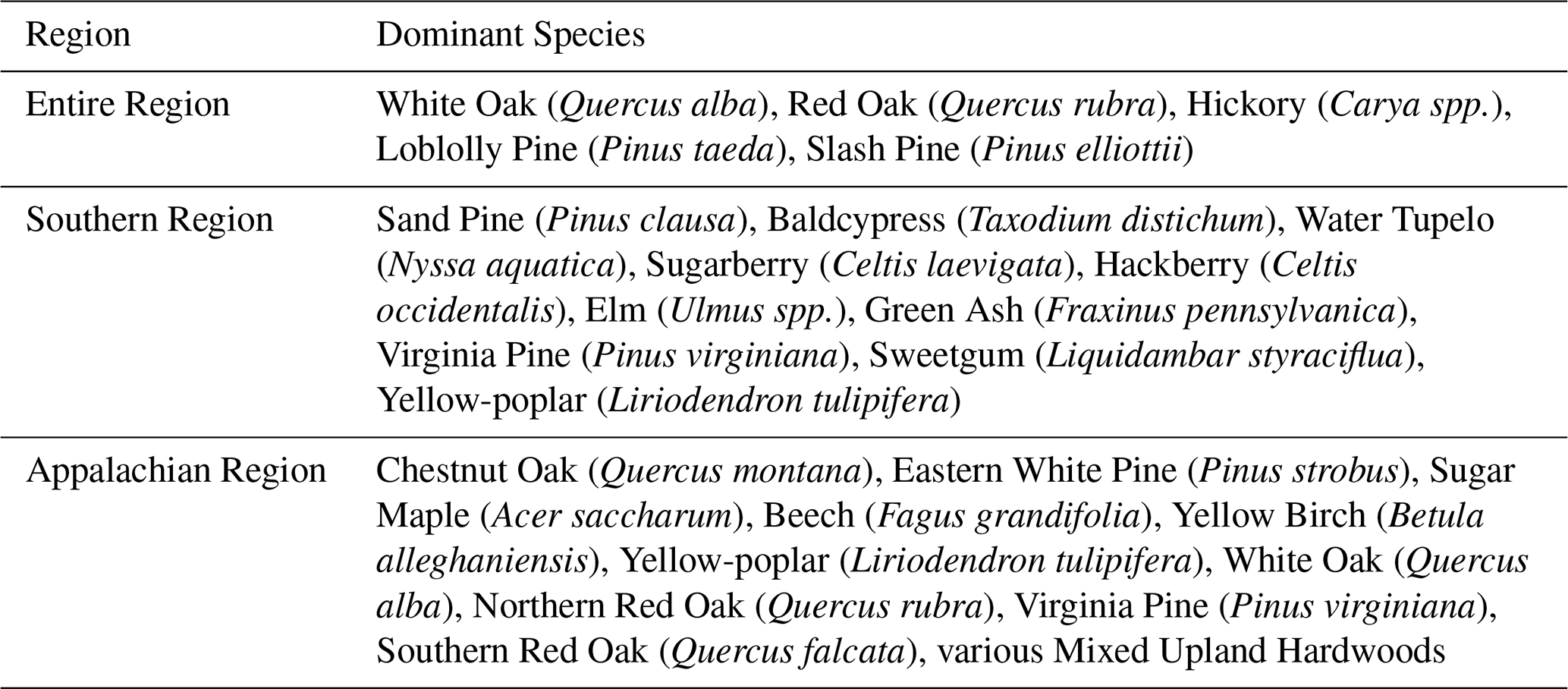
Table A2Equi7 Sentinel-1 Change Detection Grid Cells used over the region in North America, downloaded from Sentinel-1.
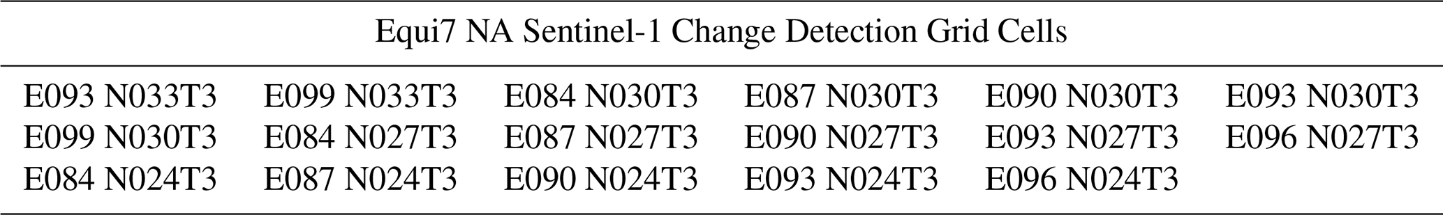
Table A3Event filtering workflow used to derive the final disturbance dataset. Counts represent the number of disturbance events before and after each filtering step. Two branches are created after compound-event detection: (a) compound-free disturbance events and (b) recurring disturbance events occurring within two years.
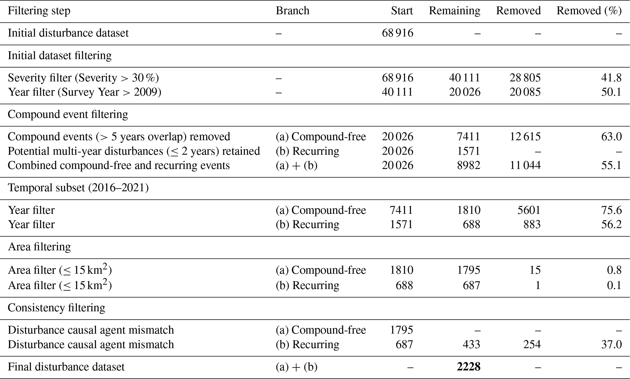
Table A4Key columns in the S1DM geodataframe, documenting attributes of the disturbance events recorded by IDS and detected via the S1CD radar satellite.
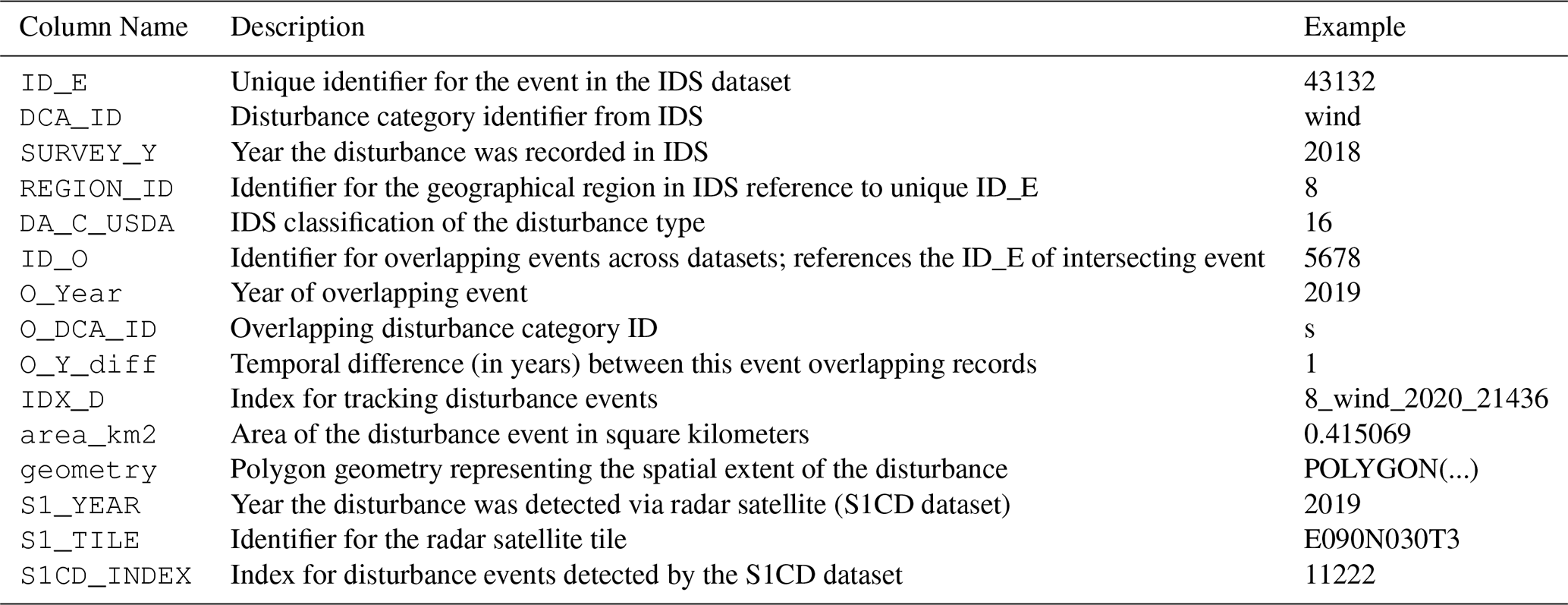
Table A5Codes of the 28 major disturbance-agent categories used in the IDS Damage Causal Agent (DCA) classification, along with the number of subcategories defined under each category and selected examples of subgroups, as described in the Aerial Survey Geographic Information System Handbook of the U.S. Forest Service (USDA Forest Service, 2005).
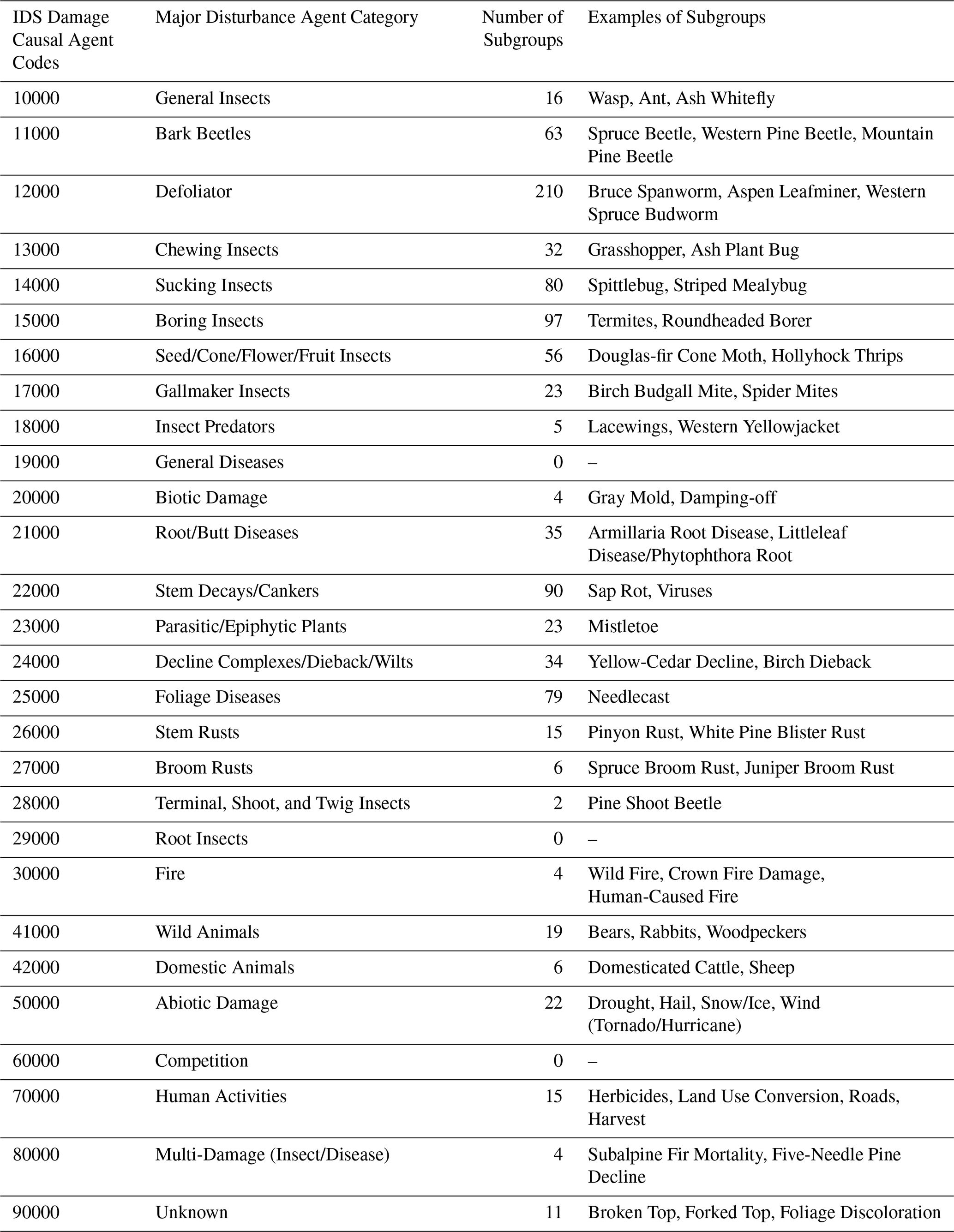
Table A6Median Intersection over Union (IoU) and area overlap (%) for IDS and S1DM polygons compared to manually labelled references.
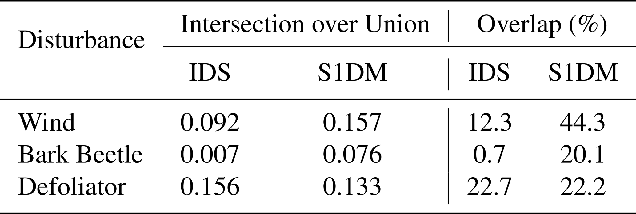
The code is publicly availabe on https://github.com/Franziska279/ForExD-WP1-P1 (last access: 10 June 2026).
Insect and Disease Survey data by the U.S. Department of Agriculture can be downloaded at https://www.fs.usda.gov/science-technology/data-tools-products/fhp-mapping-reporting/detection-surveys (last access: 1 June 2026); Tree Canopy Cover data from the U.S. Forest Service’s Geospatial Technology and Applications Center is available at https://data.fs.usda.gov/geodata/rastergateway/treecanopycover/ (last access: 1 June 2026). The Sentinel-1 change detection dataset (S1CD) is available at https://doi.org/10.5281/zenodo.16903909 (Cremer and Gans, 2025) and the Sentinel-1 disturbance map (S1DM) is available at https://doi.org/10.5281/zenodo.15672487 (Müller et al., 2026).
AB and FM designed the study. LE performed IDS data preprocessing, FC conducted Sentinel-1 Change Detection, and FM managed overall data preprocessing (IDS, S1CD, and Sentinel-2) and analysis, with scientific and technical input from AB, GCV, PB and LE. FM wrote the first draft of the paper. All authors contributed to the final manuscript.
The contact author has declared that none of the authors has any competing interests.
Publisher's note: Copernicus Publications remains neutral with regard to jurisdictional claims made in the text, published maps, institutional affiliations, or any other geographical representation in this paper. The authors bear the ultimate responsibility for providing appropriate place names. Views expressed in the text are those of the authors and do not necessarily reflect the views of the publisher.
FM and AB acknowledge funding by the European Union (ERC StG, ForExD, grant agreement No. 101039567). GC-V thanks funding from the European Research Council (ERC) under the ERC Synergy Grant USMILE (grant agreement 855187) and the H2020 project XAIDA (grant agreement 101003469). This work uses Copernicus Sentinel data 2016-2022. The generation of the S1CD data was supported by the ESA Network of Resources Initiative and the Copernicus – eoSC AnaLytics Engine (C-SCALE) project, which received funding from the European Union's Horizon 2020 research and innovation program under grant agreement No. 101017529. The views expressed are purely those of the writers and may not in any circumstances be regarded as stating an official position of the European Commission.
This work was supported by the HORIZON EUROPE European Research Council under the projects ForExD (Forest vulnerability to compound extremes and disturbances in a changing climate, grant no. 101039567) and USMILE (Understanding and Modelling the Earth System with Machine Learning, grant no. 855187), by the European Union under the projects XAIDA (eXtreme events: Artificial Intelligence for Detection and Attribution, grant no. 101003469) and C-SCALE (Copernicus – eoSC AnaLytics Engine, grant no. 101017529), by the European Space Agency through the ESA Network of Resources, and by Schmidt Futures (grant no. G-23-64959).
Supported by the Open Access Publishing Fund
of Leipzig University.
This paper was edited by Mihai Niculita and reviewed by two anonymous referees.
Aloisi, A.: Commoditized Workers. Case Study Research on Labour Law Issues Arising from a Set of “On-Demand/Gig Economy” Platforms, https://doi.org/10.2139/ssrn.2637485, 2016. a
Altman, J., Fibich, P., Trotsiuk, V., and Altmanova, N.: Global pattern of forest disturbances and its shift under climate change, Sci. Total Environ., 915, 170117, https://doi.org/10.1016/j.scitotenv.2024.170117, 2024. a
Anderegg, W. R. L., Hicke, J. A., Fisher, R. A., Allen, C. D., Aukema, J., Bentz, B., Hood, S., Lichstein, J. W., Macalady, A. K., Mcdowell, N., Pan, Y., Raffa, K., Sala, A., Shaw, J. D., Stephenson, N. L., Tague, C., and Zeppel, M.: Research review Tree mortality from drought, insects, and their interactions in a changing climate, New Phytol., 208, 674–683, https://doi.org/10.1111/nph.13477, 2015. a
Andresini, G., Appice, A., and Malerba, D.: A Deep Semantic Segmentation Approach to Map Forest Tree Dieback in Sentinel-2 Data, IEEE J. Sel. Top. Appl., 17, 17075–17086, https://doi.org/10.1109/JSTARS.2024.3460981, 2024. a
Andrus, R. A., Hicke, J. A., and Meddens, A. J. H.: Spatiotemporal characteristics of tree mortality from bark beetle outbreaks vary within and among bark beetle-host tree associations in the western United States, Forest Ecol. Manag., 576, 122382, https://doi.org/10.1016/j.foreco.2024.122382, 2025. a
Backsen, J. C. and Howell, B.: Comparing Aerial Detection and Photo Interpretation for Conducting Forest Health Surveys, West. J. Appl. For., 28, 3–8, https://doi.org/10.5849/wjaf.12-010, 2013. a, b
Bae, S., Müller, J., Förster, B., Hilmers, T., Hochrein, S., Jacobs, M., Leroy, B. M. L., Pretzsch, H., Weisser, W. W., and Mitesser, O.: Tracking the temporal dynamics of insect defoliation by high-resolution radar satellite data, Methods Ecol. Evol., 13, 121–132, https://doi.org/10.1111/2041-210X.13726, 2022. a
Bauer-Marschallinger, B., Sabel, D., and Wagner, W.: Optimisation of global grids for high-resolution remote sensing data, Comput. Geosci., 72, 84–93, https://doi.org/10.1016/j.cageo.2014.07.005, 2014. a
Bauman, D., Fortunel, C., Delhaye, G., Malhi, Y., Cernusak, L. A., Bentley, L. P., Rifai, S. W., Aguirre-Gutiérrez, J., Menor, I. O., Phillips, O. L., McNellis, B. E., Bradford, M., Laurance, S. G. W., Hutchinson, M. F., Dempsey, R., Santos-Andrade, P. E., Ninantay-Rivera, H. R., Chambi Paucar, J. R., and McMahon, S. M.: Tropical tree mortality has increased with rising atmospheric water stress, Nature, 608, 528–533, https://doi.org/10.1038/s41586-022-04737-7, 2022. a
Baumann, M., Ozdogan, M., Wolter, P. T., Krylov, A., Vladimirova, N., and Radeloff, V. C.: Landsat remote sensing of forest windfall disturbance, Remote Sens. Environ., 143, 171–179, https://doi.org/10.1016/j.rse.2013.12.020, 2014. a
Borlaf-Mena, I., Santoro, M., Villard, L., Badea, O., and Tanase, M.: Investigating the Impact of Digital Elevation Models on Sentinel-1 Backscatter and Coherence Observations, Remote Sens., 12, 3016, https://doi.org/10.3390/rs12183016, 2020. a
Bruggisser, M., Dorigo, W., Dostálová, A., Hollaus, M., Navacchi, C., Schlaffer, S., and Pfeifer, N.: Potential of Sentinel-1 C-Band Time Series to Derive Structural Parameters of Temperate Deciduous Forests, Remote Sens., 13, 798, https://doi.org/10.3390/rs13040798, 2021. a
Byrne, B., Liu, J., Bowman, K. W., Pascolini-Campbell, M., Chatterjee, A., Pandey, S., Miyazaki, K., van der Werf, G. R., Wunch, D., Wennberg, P. O., Roehl, C. M., and Sinha, S.: Carbon emissions from the 2023 Canadian wildfires, Nature, 633, 835–839, https://doi.org/10.1038/s41586-024-07878-z, 2024. a
Bárta, V., Lukeš, P., and Homolová, L.: Early detection of bark beetle infestation in Norway spruce forests of Central Europe using Sentinel-2, Int. J. Appl. Earth Obs., 100, 102335, https://doi.org/10.1016/j.jag.2021.102335, 2021. a
Canadell, J. G., Meyer, C. P. M., Cook, G. D., Dowdy, A., Briggs, P. R., Knauer, J., Pepler, A., and Haverd, V.: Multi-decadal increase of forest burned area in Australia is linked to climate change, Nat. Commun., 12, 6921, https://doi.org/10.1038/s41467-021-27225-4, 2021a. a
Canadell, J. G., Monteiro, P. M., Costa, M. H., Cotrim da Cunha, L., Cox, P. M., Eliseev, A. V., Hensen, S., Ishii, M., Jaccard, S., Koven, C., Lohila, A., Patra, P. K., Piao, S., Rogelj, J., Syampungani, S., Zaehle, S., and Zickfeld, K.: Global carbon and other biogeochemical cycles and feedbacks, IPCC, https://doi.org/10.1017/9781009157896.007, 2021b. a
Candotti, A., De Giglio, M., Dubbini, M., and Tomelleri, E.: A Sentinel-2 Based Multi-Temporal Monitoring Framework for Wind and Bark Beetle Detection and Damage Mapping, Remote Sens., 14, 6105, https://doi.org/10.3390/rs14236105, 2022. a, b
Chen, X., Zhao, W., Chen, J., Qu, Y., Wu, D., and Chen, X.: Mapping Large-Scale Forest Disturbance Types with Multi-Temporal CNN Framework, Remote Sens., 13, https://doi.org/10.3390/rs13245177, 2021. a
Chuvieco, E., Lizundia-Loiola, J., Pettinari, M. L., Ramo, R., Padilla, M., Tansey, K., Mouillot, F., Laurent, P., Storm, T., Heil, A., and Plummer, S.: Generation and analysis of a new global burned area product based on MODIS 250 m reflectance bands and thermal anomalies, Earth Syst. Sci. Data, 10, 2015–2031, https://doi.org/10.5194/essd-10-2015-2018, 2018. a
Cohen, W. B., Yang, Z., and Kennedy, R. E.: Detecting trends in forest disturbance and recovery using yearly Landsat time series: 2. Time series analysis, Remote Sens. Environ., 114, 2897–2910, https://doi.org/10.1016/j.rse.2010.07.010, 2010. a
Coleman, T. W., Graves, A. D., Heath, Z., Flowers, R. W., Hanavan, R. P., Cluck, D. R., and Ryerson, D.: Accuracy of aerial detection surveys for mapping insect and disease disturbances in the United States, Forest Ecol. Manag., 430, 321–336, https://doi.org/10.1016/j.foreco.2018.08.020, 2018. a, b, c, d, e, f, g, h
Cremer, F. and Gans, F.: Satellite-Based Forest Disturbance Dataset from Sentinel-1 SAR (2016–2021) (1.0.0), Zenodo [data set], https://doi.org/10.5281/zenodo.16903909, 2025. a
Cremer, F., Urbazaev, M., Cortés, J., Truckenbrodt, J., Schmullius, C., and Thiel, C.: Potential of Recurrence Metrics from Sentinel-1 Time Series for Deforestation Mapping, IEEE J. Sel. Top. Appl., 13, 5233–5240, https://doi.org/10.1109/JSTARS.2020.3019333, 2020. a, b, c, d, e, f, g, h
Curtis, P. G., Slay, C. M., Harris, N. L., Tyukavina, A., and Hansen, M. C.: Classifying drivers of global forest loss, Science, 361, 1108–1111, https://doi.org/10.1126/science.aau3445, 2018. a
Dalponte, M., Sassi, R., Gianelle, D., Bruzzone, L., and Marinelli, D.: Exploring the Detection of Bark Beetle Attacks in Norway Spruce Forests in Sentinel-1 Image Time Series, IEEE, https://doi.org/10.1109/IGARSS53475.2024.10641531, 2024. a
Eifler, L., Müller, F., and Bastos, A.: Evaluating the consistency of forest disturbance datasets in continental USA, Biogeosciences, 23, 1291–1325, https://doi.org/10.5194/bg-23-1291-2026, 2026. a, b, c, d, e, f, g, h, i, j, k, l
Eklundh, L., Johansson, T., and Solberg, S.: Mapping insect defoliation in Scots pine with MODIS time-series data, Remote Sens. Environ., 113, 1566–1573, https://doi.org/10.1016/j.rse.2009.03.008, 2009. a, b
ESA: ESA's Living Planet Programme: Scientific Achievements and Future Challenges – Scientific Context of the Earth Observation Science Strategy for ESA, ESA SP-1329/2, European Space Agency (ESA), Noordwijk, the Netherlands, ISBN 978-92-9221-427-2, 2015. a
European Commission: Proposal for a Regulation of the European Parliament and of the Council on a Monitoring Framework for Resilient European Forests, https://eur-lex.europa.eu/legal-content/EN/TXT/?uri=CELEX:52023PC0728, (last access: 22 November 2023), 2023. a
European Environment Agency (EU body or agency): European climate risk assessment: executive summary, Publications Office of the European Union, ISBN 978-92-9480-627-7, https://doi.org/10.2800/204249, 2024. a
FAO: Global Forest Resources Assessment 2020 (FRA2020), Tech. rep., Food and Agriculture Organization of the United Nations, Rome, https://doi.org/10.4060/ca9825en, 2020. a, b, c, d, e
Forest Service U.S. Department of Agriculture: Detection Surveys, https://www.fs.usda.gov/science-technology/data-tools-products/fhp-mapping-reporting/detection-surveys (last access: 15 August 2024), 2024. a, b, c, d
Forzieri, G., Pecchi, M., Girardello, M., Mauri, A., Klaus, M., Nikolov, C., Rüetschi, M., Gardiner, B., Tomaštík, J., Small, D., Nistor, C., Jonikavicius, D., Spinoni, J., Feyen, L., Giannetti, F., Comino, R., Wolynski, A., Pirotti, F., Maistrelli, F., Savulescu, I., Wurpillot-Lucas, S., Karlsson, S., Zieba-Kulawik, K., Strejczek-Jazwinska, P., Mokroš, M., Franz, S., Krejci, L., Haidu, I., Nilsson, M., Wezyk, P., Catani, F., Chen, Y.-Y., Luyssaert, S., Chirici, G., Cescatti, A., and Beck, P. S. A.: A spatially explicit database of wind disturbances in European forests over the period 2000–2018, Earth Syst. Sci. Data, 12, 257–276, https://doi.org/10.5194/essd-12-257-2020, 2020. a, b, c, d
Forzieri, G., Girardello, M., Ceccherini, G., Spinoni, J., Feyen, L., Hartmann, H., Beck, P. S. A., Camps-Valls, G., Chirici, G., Mauri, A., and Cescatti, A.: Emergent vulnerability to climate-driven disturbances in European forests, Nat. Commun., 12, 1081, https://doi.org/10.1038/s41467-021-21399-7, 2021. a
Forzieri, G., Dutrieux, L. P., Elia, A., Eckhardt, B., Caudullo, G., Álvarez Taboada, F., Andriolo, A., Bălăcenoiu, F., Bastos, A., Buzatu, A., Castedo Dorado, F., Dobrovolný, L., Duduman, M.-L., Fernandez-Carrillo, A., Cescatti, A., A Beck, P. S., Giovanni Forzieri, C., and Commission, E.: The Database of European Forest Insect and Disease Disturbances: DEFID2, Glob. Change Biol., https://doi.org/10.1111/gcb.16912, 2023. a, b, c, d, e
Gibson, R., Danaher, T., Hehir, W., and Collins, L.: A remote sensing approach to mapping fire severity in south-eastern Australia using sentinel 2 and random forest, Remote Sens. Environ., 240, 111702, https://doi.org/10.1016/j.rse.2020.111702, 2020. a
Graziosi, I., Tembo, M., Kuate, J., and Muchugi, A.: Pests and diseases of trees in Africa: A growing continental emergency, Plants, People, Planet, 2, 14–28, https://doi.org/10.1002/ppp3.31, 2020. a
Hall, R., Castilla, G., White, J., Cooke, B., and Skakun, R.: Remote sensing of forest pest damage: a review and lessons learned from a Canadian perspective, Can. Entomol., 148, S296–S356, https://doi.org/10.4039/tce.2016.11, 2016. a, b, c, d
Hammond, W. M., H., Williams, A. P., Abatzoglou, J. T., Adams, H. D., Klein, T., López Rodríguez, R., Sáenz-Romero, C., Hartmann, H., Breshears, D. D., and Allen, C. D.: Global field observations of tree die-off reveal hotter-drought fingerprint for Earth's forests, Nat. Commun., 13, 1761, https://doi.org/10.1038/s41467-022-29289-2, 2022. a
Hansen, M., Potapov, P. V., Moore, R., Hancher, M., Turubanova, S., Tyukavina, A., Thau, D., Stehman, S., Goetz, S., Loveland, T., Kommareddy, A., Egorov, A., Chini, L., Justice, C., and Townshed, J.: Global Forest Change 2000–2024 Data Download, https://storage.googleapis.com/earthenginepartners-hansen/GFC-2024-v1.12/download.html (last access: 22 July 2024), 2024. a
Hansen, M. C. and Loveland, T. R.: A review of large area monitoring of land cover change using Landsat data, Remote Sens. Environ., 122, 66–74, https://doi.org/10.1016/j.rse.2011.08.024, 2012. a
Hansen, M. C., Potapov, P. V., Moore, R., Hancher, M., Turubanova, S. A., Tyukavina, A., Thau, D., Stehman, S. V., Goetz, S. J., Loveland, T. R., Kommareddy, A., Egorov, A., Chini, L., Justice, C. O., and Townshend, J. R.: High-resolution global maps of 21st-century forest cover change, Science, 342, 850–853, https://doi.org/10.1126/SCIENCE.1244693, 2013. a
Harris, N. L., Brown, S., Hagen, S. C., Saatchi, S. S., Petrova, S., Salas, W., Hansen, M. C., Potapov, P. V., and Lotsch, A.: Baseline Map of Carbon Emissions from Deforestation in Tropical Regions, Science, 336, 1573–1576, https://doi.org/10.1126/science.1217962, 2012. a
Harris, N. L., Hagen, S. C., Saatchi, S. S., Pearson, T. R. H., Woodall, C. W., Domke, G. M., Braswell, B. H., Walters, B. F., Brown, S., Salas, W., Fore, A., and Yu, Y.: Attribution of net carbon change by disturbance type across forest lands of the conterminous United States, Carbon Balance and Management, 11, 24, https://doi.org/10.1186/s13021-016-0066-5, 2016. a, b, c, d, e
Hartmann, H., Bastos, A., Das, A. J., Esquivel-Muelbert, A., Hammond, W. M., Martínez-Vilalta, J., McDowell, N. G., Powers, J. S., Pugh, T. A., and Ruthrof, K. X.: Climate change risks to global forest health: emergence of unexpected events of elevated tree mortality worldwide, Annu. Rev. Plant Biolo., 73, 673–702, 2022. a
Hawkins, W. and Mittelstadt, B.: The ethical ambiguity of AI data enrichment: Measuring gaps in research ethics norms and practices, in: Proceedings of the 2023 ACM Conference on Fairness, Accountability, and Transparency, FAccT '23, pp. 261–270, Association for Computing Machinery, New York, NY, USA, ISBN 979-8-4007-0192-4, https://doi.org/10.1145/3593013.3593995, 2023. a
Hawryło, P., Bednarz, B., Wężyk, P., and Szostak, M.: Estimating defoliation of Scots pine stands using machine learning methods and vegetation indices of Sentinel-2, Eur. J. Remote Sens., 51, 194–204, https://doi.org/10.1080/22797254.2017.1417745, 2018. a
Heaton, R., Song, B., Williams, T., Conner, W., Baucom, Z., and Williams, B.: Twenty-Seven Year Response of South Carolina Coastal Plain Forests Affected by Hurricane Hugo, Plants, 12, 691, https://doi.org/10.3390/plants12040691, 2023. a, b
Heinrich, V. H. A., Dalagnol, R., Cassol, H. L. G., Rosan, T. M., de Almeida, C. T., Silva Junior, C. H. L., Campanharo, W. A., House, J. I., Sitch, S., Hales, T. C., Adami, M., Anderson, L. O., and Aragão, L. E. O. C.: Large carbon sink potential of secondary forests in the Brazilian Amazon to mitigate climate change, Nat. Commun., 12, 1785, https://doi.org/10.1038/s41467-021-22050-1, 2021. a
Helbig, C. E., Müller, M. G., and Landgraf, D.: Effects of Leaf Loss by Artificial Defoliation on the Growth of Different Poplar and Willow Varieties, Forests, 12, https://doi.org/10.3390/f12091224, 2021. a
Helmer, E. H., Ruzycki, T. S., Wunderle Jr., J. M., Vogesser, S., Ruefenacht, B., Kwit, C., Brandeis, T. J., and Ewert, D. N.: Mapping tropical dry forest height, foliage height profiles and disturbance type and age with a time series of cloud-cleared Landsat and ALI image mosaics to characterize avian habitat, Remote Sens. Environ., 114, 2457–2473, https://doi.org/10.1016/j.rse.2010.05.021, 2010. a
Hicke, J. A., Allen, C. D., Desai, A. R., Dietze, M. C., Hall, R. J., Kashian, D. M., Moore, D., Raffa, K. F., Sturrock, R. N., Vogelmann, J., and others: Effects of biotic disturbances on forest carbon cycling in the United States and Canada, Glob. Change Biol., 18, 7–34, 2012. a
Hicke, J. A., Meddens, A. J., and Kolden, C. A.: Recent Tree Mortality in the Western United States from Bark Beetles and Forest Fires, Forest Sci., 62, 141–153, https://doi.org/10.5849/forsci.15-086, 2016. a, b
Hicke, J. A., Xu, B., Meddens, A. J. H., and Egan, J. M.: Characterizing recent bark beetle-caused tree mortality in the western United States from aerial surveys, Forest Ecol. Manag., 475, 118402, https://doi.org/10.1016/j.foreco.2020.118402, 2020. a, b, c
Hirschmugl, M., Gallaun, H., Dees, M., Datta, P., Deutscher, J., Koutsias, N., and Schardt, M.: Methods for Mapping Forest Disturbance and Degradation from Optical Earth Observation Data: a Review, Current Forestry Reports, 3, 32–45, https://doi.org/10.1007/s40725-017-0047-2, 2017. a
Housman, I. W., Heyer, J. P., Ruefenacht, B., Schleeweis, K., Megown, K., Bogle, S., Reischmann, J., and Ryerson, D.: National Land Cover Database Tree Canopy Cover Methods v2023.5, Technical Report GO-10268-RPT2, U.S. Department of Agriculture, Forest Service, Field Services and Innovation Center–Geospatial Office, Salt Lake City, UT, https://data.fs.usda.gov/geodata/rastergateway/treecanopycover/docs/TCC_v2023-5_Methods.pdf (last access: 1 June 2026), 2025. a
Huang, X., Ziniti, B., Torbick, N., and Ducey, M. J.: Assessment of Forest above Ground Biomass Estimation Using Multi-Temporal C-band Sentinel-1 and Polarimetric L-band PALSAR-2 Data, Remote Sens., 10, https://doi.org/10.3390/rs10091424, 2018. a
Imperatore, P.: SAR Imaging Distortions Induced by Topography: A Compact Analytical Formulation for Radiometric Calibration, Remote Sens., 13, 3318, https://doi.org/10.3390/rs13163318, 2021. a
Jaccard, P.: Lois de distribution florale dans la zone alpine, Bulletin de la Société Vaudoise des Sciences Naturelles, 38, https://doi.org/10.5169/SEALS-266762, 1902. a
Jones, M. W., Abatzoglou, J. T., Veraverbeke, S., Andela, N., Lasslop, G., Forkel, M., Smith, A. J. P., Burton, C., Betts, R. A., van der Werf, G. R., Sitch, S., Canadell, J. G., Santín, C., Kolden, C., Doerr, S. H., and Le Quéré, C.: Global and Regional Trends and Drivers of Fire Under Climate Change, Rev. Geophys., 60, e2020RG000726, https://doi.org/10.1029/2020RG000726, 2022. a
Justice, C., Vermote, E., Townshend, J., Defries, R., Roy, D., Hall, D., Salomonson, V., Privette, J., Riggs, G., Strahler, A., Lucht, W., Myneni, R., Knyazikhin, Y., Running, S., Nemani, R., Wan, Z., Huete, A., van Leeuwen, W., Wolfe, R., Giglio, L., Muller, J., Lewis, P., and Barnsley, M.: The Moderate Resolution Imaging Spectroradiometer (MODIS): land remote sensing for global change research, IEEE T. Geosci. Remote, 36, 1228–1249, https://doi.org/10.1109/36.701075, 1998. a
Karel, T. H. and Man, G.: Major forest insect and disease conditions in the United States: 2015, 45 pp., U.S. Department of Agriculture, Forest Service, https://www.fs.usda.gov/foresthealth/publications/ConditionsReport_2015.pdf (last access: 10 June 2026), 2017. a
Kautz, M.: On correcting the time-lag bias in aerial-surveyed bark beetle infestation data, Forest Ecol. Manag., 326, 157–162, https://doi.org/10.1016/j.foreco.2014.04.010, 2014. a, b, c, d, e
Kautz, M., Meddens, A. J. H., Hall, R. J., and Arneth, A.: Biotic disturbances in Northern Hemisphere forests-a synthesis of recent data, uncertainties and implications for forest monitoring and modelling, Global Ecol. Biogeogr., 26, 533–552, https://doi.org/10.1111/geb.12558, 2017. a, b, c, d, e, f, g, h
Kautz, M., Anthoni, P., Meddens, A. J. H., Pugh, T. A. M., and Arneth, A.: Simulating the recent impacts of multiple biotic disturbances on forest carbon cycling across the United States, Glob. Change Biol., 24, 2079–2092, https://doi.org/10.1111/gcb.13974, 2018. a
Kautz, M., Feurer, J., and Adler, P.: Early detection of bark beetle (Ips typographus) infestations by remote sensing – A critical review of recent research, Forest Ecol. Manag., 556, 121595, https://doi.org/10.1016/j.foreco.2023.121595, 2024. a, b
Kellndorfer, J.: Using SAR data for mapping deforestation and forest degradation, in: Synthetic Aperture Radar (SAR) Handbook: Comprehensive Methodologies for Forest Monitoring and Biomass Estimation, edited by: Flores-Anderson, A. I., Herndon, K. E., Thapa, R. B., and Cherrington, E., chap. 3, SERVIR Global Science Coordination Office, National Space Science and Technology Center, Huntsville, AL, 47–66, https://doi.org/10.25966/nr2c-s697, 2019. a
Kennedy, R. E., Yang, Z., and Cohen, W. B.: Detecting trends in forest disturbance and recovery using yearly Landsat time series: 1. LandTrendr – Temporal segmentation algorithms, Remote Sens. Environ., 114, 2897–2910, https://doi.org/10.1016/j.rse.2010.07.008, 2010. a
Kislov, D. E., Korznikov, K. A., Altman, J., Vozmishcheva, A. S., and Krestov, P. V.: Extending deep learning approaches for forest disturbance segmentation on very high-resolution satellite images, Remote Sensing in Ecology and Conservation, 7, 355–368, https://doi.org/10.1002/rse2.194, 2021. a
Konings, A. G., Saatchi, S. S., Frankenberg, C., Keller, M., Leshyk, V., Anderegg, W. R. L., Humphrey, V., Matheny, A. M., Trugman, A., Sack, L., Agee, E., Barnes, M. L., Binks, O., Cawse-Nicholson, K., Christoffersen, B. O., Entekhabi, D., Gentine, P., Holtzman, N. M., Katul, G. G., Liu, Y., Longo, M., Martinez-Vilalta, J., McDowell, N., Meir, P., Mencuccini, M., Mrad, A., Novick, K. A., Oliveira, R. S., Siqueira, P., Steele-Dunne, S. C., Thompson, D. R., Wang, Y., Wehr, R., Wood, J. D., Xu, X., and Zuidema, P. A.: Detecting forest response to droughts with global observations of vegetation water content, Glob. Change Biol., 27, 6005–6024, https://doi.org/10.1111/gcb.15872, 2021. a
Korosuo, A., Pilli, R., Abad Viñas, R., Blujdea, V. N. B., Colditz, R. R., Fiorese, G., Rossi, S., Vizzarri, M., and Grassi, G.: The role of forests in the EU climate policy: are we on the right track?, Carbon Balance and Management, 18, 15, https://doi.org/10.1186/s13021-023-00234-0, 2023. a
Kurz, W. A., Dymond, C. C., Stinson, G., Rampley, G. J., Neilson, E. T., Carroll, A. L., Ebata, T., and Safranyik, L.: Mountain pine beetle and forest carbon feedback to climate change, Nature, 452, 987–990, https://doi.org/10.1038/nature06777, 2008. a
Markham, B. L. and Helder, D. L.: Forty-year calibrated record of earth-reflected radiance from Landsat: A review, Remote Sens. Environ., 122, 30–40, https://doi.org/10.1016/j.rse.2011.06.026, 2012. a
Marwan, N., Romano, M. C., Thiel, M., and Kurths, J.: Recurrence Plots for the Analysis of Complex Systems, Phys. Rep., 438, 237–329, https://doi.org/10.1016/j.physrep.2006.11.001, 2007. a
McConnell, T. J.: A Guide to Conducting Aerial Sketchmapping Surveys, U.S. Department of Agriculture, Forest Service, Forest Health Technology Enterprise Team, U.S. Department of Agriculture internal, https://www.fs.usda.gov/foresthealth/technology/pdfs/Sketchmapping.pdf (last access: 10 June 2026), 2000. a, b, c, d
McDowell, N. G., Coops, N. C., Beck, P. S., Chambers, J. Q., Gangodagamage, C., Hicke, J. A., Huang, C.-y., Kennedy, R., Krofcheck, D. J., Litvak, M., Meddens, A. J., Muss, J., Negrón-Juarez, R., Peng, C., Schwantes, A. M., Swenson, J. J., Vernon, L. J., Williams, A. P., Xu, C., Zhao, M., Running, S. W., and Allen, C. D.: Global satellite monitoring of climate-induced vegetation disturbances, Trends Plant Sci., 20, 114–123, 2015. a, b, c, d, e, f, g
McDowell, N. G., Allen, C. D., Anderson-Teixeira, K., Aukema, B. H., Bond-Lamberty, B., Chini, L., Clark, J. S., Dietze, M., Grossiord, C., Hanbury-Brown, A., Hurtt, G. C., Jackson, R. B., Johnson, D. J., Kueppers, L., Lichstein, J. W., Ogle, K., Poulter, B., Pugh, T. A. M., Seidl, R., Turner, M. G., Uriarte, M., Walker, A. P., and Xu, C.: Pervasive shifts in forest dynamics in a changing world, Science, 368, eaaz9463, https://doi.org/10.1126/science.aaz9463, 2020. a, b
Meddens, A. J. H., Hicke, J. A., and Ferguson, C. A.: Spatiotemporal patterns of observed bark beetle-caused tree mortality in British Columbia and the western United States, Ecol. Appl., 22, 1876–1891, 2012. a, b
Migliavacca, M., Grassi, G., Bastos, A., Ceccherini, G., Ciais, P., Janssens-Maenhout, G., Lugato, E., Mahecha, M., Novick, K., Peñuelas, J., Pilli, R., Reichstein, M., Avitabile, V., Beck, P. S. A., Barredo, J. I., Forzieri, G., Herold, M., Korosuo, A., Mansuy, N., Mubareka, S., Orth, R., Rougieux, P., and Cescatti, A.: Securing the forest carbon sink for the European Union’s climate ambition: Scientific action to anticipate the evolution of the forest carbon sink, Nature, 643, 1203–1213, https://doi.org/10.1038/s41586-025-08967-3, 2025. a
Mitchell, S. J.: Wind as a natural disturbance agent in forests: a synthesis, Forestry, 86, 147–157, https://doi.org/10.1093/forestry/cps058, 2013. a
Müller, F., Eifler, L., Cremer, F., Beck, P. S. A., Camps-Valls, G., and Bastos, A.: Sentinel-1 Disturbance Map. In Natural Hazards and Earth System Sciences (NHESS) (1.0.0), European Geosciences Union General Assembly 2024 (EGU 2024), Vienna, Zenodo [data set], https://doi.org/10.5281/zenodo.15672487, 2026. a
Nabuurs, G.-J., Lindner, M., Verkerk, H., Gunia, K., Deda, P., Michalak, R., and Grassi, G.: First signs of carbon sink saturation in European forest biomass, Nat. Clim. Change, 3, https://doi.org/10.1038/nclimate1853, 2013. a
Negrón-Juárez, R. I., Holm, J. A., Marra, D. M., Rifai, S. W., Riley, W. J., Chambers, J. Q., Koven, C. D., Knox, R. G., McGroddy, M. E., Vittorio, A. V. D., Urquiza-Muñoz, J., Tello-Espinoza, R., Muñoz, W. A., Ribeiro, G. H. P. M., and Higuchi, N.: Vulnerability of Amazon forests to storm-driven tree mortality, Environ. Res. Lett., 13, 054021, https://doi.org/10.1088/1748-9326/aabe9f, 2018. a, b
Oeser, J., Pflugmacher, D., Senf, C., Heurich, M., and Hostert, P.: Using Intra-Annual Landsat Time Series for Attributing Forest Disturbance Agents in Central Europe, Forests, 8, 251, https://doi.org/10.3390/f8070251, 2017. a
Pan, Y., Birdsey, R. A., Phillips, O. L., Houghton, R. A., Fang, J., Kauppi, P. E., Keith, H., Kurz, W. A., Ito, A., Lewis, S. L., Nabuurs, G.-J., Shvidenko, A., Hashimoto, S., Lerink, B., Schepaschenko, D., Castanho, A., and Murdiyarso, D.: The enduring world forest carbon sink, Nature, 631, 563–569, https://doi.org/10.1038/s41586-024-07602-x, 2024. a
Patacca, M., Schelhaas, M.-J., Zudin, S., and Lindner, M.: Database on Forest Disturbances in Europe (DFDE)-Technical report History, State of the Art, and Future Perspectives, Project I-Maestro (ERA-NET Cofund ForestValue), 2021. a, b
PBC, P. L.: Education and Research Program –Planet, https://www.planet.com/industries/education-and-research/ (last access: 20 October 2025), 2025. a, b
Popp, T., Hegglin, M. I., Hollmann, R., Ardhuin, F., Bartsch, A., Bastos, A., Bennett, V., Boutin, J., Brockmann, C., Buchwitz, M., Chuvieco, E., Ciais, P., Dorigo, W., Ghent, D., Jones, R., Lavergne, T., Merchant, C. J., Meyssignac, B., Paul, F., Quegan, S., Sathyendranath, S., Scanlon, T., Schröder, M., Simis, S. G. H., and Willén, U.: Consistency of Satellite Climate Data Records for Earth System Monitoring, B. Am. Meteor. Soc., 101, E1948–E1971, https://doi.org/10.1175/BAMS-D-19-0127.1, 2020. a
Richter, R., Ballasus, H., Engelmann, R. A., Zielhofer, C., Sanaei, A., and Wirth, C.: Tree species matter for forest microclimate regulation during the drought year 2018: disentangling environmental drivers and biotic drivers, Sci. Re., 12, 17559, https://doi.org/10.1038/s41598-022-22582-6, 2022. a
Rodríguez Paulino, E., Schlerf, M., Röder, A., Stoffels, J., and Udelhoven, T.: Forest disturbance characterization in the era of earth observation big data: A mapping review, Int. J. Appl. Earth Obs., 128, 103755, https://doi.org/10.1016/j.jag.2024.103755, 2024. a, b
Rüetschi, M., Small, D., and Waser, L. T.: Rapid Detection of Windthrows Using Sentinel-1 C-Band SAR Data, Remote Sens., 11, 115, https://doi.org/10.3390/rs11020115, 2019. a
Schleeweis, K. G., Moisen, G. G., Schroeder, T. A., Toney, C., Freeman, E. A., Goward, S. N., Huang, C., and Dungan, J. L.: US National Maps Attributing Forest Change: 1986–2010, Forests, 11, 653, https://doi.org/10.3390/f11060653, 2020. a, b, c
Schuldt, B., Buras, A., Arend, M., Vitasse, Y., Beierkuhnlein, C., Damm, A., Gharun, M., Grams, T. E. E., Hauck, M., Hajek, P., Hartmann, H., Hiltbrunner, E., Hoch, G., Holloway-Phillips, M., Körner, C., Larysch, E., Lübbe, T., Nelson, D. B., Rammig, A., Rigling, A., Rose, L., Ruehr, N. K., Schumann, K., Weiser, F., Werner, C., Wohlgemuth, T., Zang, C. S., and Kahmen, A.: A first assessment of the impact of the extreme 2018 summer drought on Central European forests, Basic Appl. Ecol., 45, 86–103, https://doi.org/10.1016/j.baae.2020.04.003, 2020. a
Seidl, R. and Turner, M. G.: Post-disturbance reorganization of forest ecosystems in a changing world, P. Natl. Acad. Sci. USA, 119, e2202190119, https://doi.org/10.1073/pnas.2202190119, 2022. a
Seidl, R., Schelhaas, M.-J., Rammer, W., and Verkerk, P. J.: Increasing forest disturbances in Europe and their impact on carbon storage, Nat. Clim. Change, 4, 806–810, 2014. a, b
Seidl, R., Thom, D., Kautz, M., Martin-Benito, D., Peltoniemi, M., Vacchiano, G., Wild, J., Ascoli, D., Petr, M., Honkaniemi, J., Lexer, M. J., Trotsiuk, V., Mairota, P., Svoboda, M., Fabrika, M., Nagel, T. A., and Reyer, C. P.: Forest disturbances under climate change, Nat. Clim. Change, 7, 395–402, https://doi.org/10.1038/NCLIMATE3303, 2017. a, b
Senf, C. and Seidl, R.: Natural disturbances are spatially diverse but temporally synchronized across temperate forest landscapes in Europe, Glob. Change Biol., 24, 1201–1211, https://doi.org/10.1111/gcb.13897, 2018. a, b, c, d
Senf, C. and Seidl, R.: Persistent impacts of the 2018 drought on forest disturbance regimes in Europe, Biogeosciences, 18, 5223–5230, https://doi.org/10.5194/bg-18-5223-2021, 2021a. a
Senf, C. and Seidl, R.: Storm and fire disturbances in Europe: Distribution and trends, Glob. Change Biol., 27, 3605–3619, https://doi.org/10.1111/gcb.15679, 2021b. a, b
Senf, C., Pflugmacher, D., Wulder, M. A., and Hostert, P.: Characterizing spectral-temporal patterns of defoliator and bark beetle disturbances using Landsat time series, Remote Sens. Environ., 170, 166–177, https://doi.org/10.1016/j.rse.2015.09.019, 2015. a, b, c, d
Senf, C., Müller, J., and Seidl, R.: Post-disturbance recovery of forest cover and tree height differ with management in Central Europe, Landscape Ecol., 34, 2837–2850, https://doi.org/10.1007/s10980-019-00921-9, 2019. a
Senf, C., Buras, A., Zang, C. S., Rammig, A., and Seidl, R.: Excess forest mortality is consistently linked to drought across Europe, Nat. Commun., 11, 6200, https://doi.org/10.1038/s41467-020-19924-1, 2020. a
Shi, C., Zuo, X., Zhang, J., Zhu, D., Li, Y., and Bu, J.: Accuracy Assessment of Geometric-Distortion Identification Methods for Sentinel-1 Synthetic Aperture Radar Imagery in Highland Mountainous Regions, Sensors, 24, 2834, https://doi.org/10.3390/s24092834, 2024. a
Small, D.: Flattening Gamma: Radiometric Terrain Correction for SAR Imagery, IEEE T. Geosci. Remote, 49, 3081–3093, https://doi.org/10.1109/TGRS.2011.2120616, 2011. a
Stahl, A. T., Andrus, R., Hicke, J. A., Hudak, A. T., Bright, B. C., and Meddens, A. J. H.: Automated attribution of forest disturbance types from remote sensing data: A synthesis, Remote Sens. Environ., 285, 113416, https://doi.org/10.1016/j.rse.2022.113416, 2023. a
Tanase, M. A., Villard, L., Pitar, D., Apostol, B., Petrila, M., Chivulescu, S., Leca, S., Borlaf-Mena, I., Pascu, I.-S., Dobre, A.-C., Pitar, D., Guiman, G., Lorent, A., Anghelus, C., Ciceu, A., Nedea, G., Stanculeanu, R., Popescu, F., Aponte, C., and Badea, O.: Synthetic aperture radar sensitivity to forest changes: A simulations-based study for the Romanian forests, Sci. Total Environ., 689, 1104–1114, 2019. a
Thom, D. and Seidl, R.: Natural disturbance impacts on ecosystem services and biodiversity in temperate and boreal forests, Biol. Rev., 91, 760–781, https://doi.org/10.1111/brv.12193, 2016. a
Torres, R., Snoeij, P., Geudtner, D., Bibby, D., Davidson, M., Attema, E., Potin, P., Rommen, B., Floury, N., Brown, M., Navas Traver, I., Deghaye, P., Duesmann, B., Rosich, B., Miranda, N., Bruno, C., L'Abbate, M., Croci, R., Pietropaolo, A., Huchler, M., and Rostan, F.: GMES Sentinel-1 mission, Remote Sens. Environ., 120, 9–24, https://doi.org/10.1016/j.rse.2011.05.028, 2012. a, b
Trumbore, S., Brando, P., and Hartmann, H.: Forest health and global change, Science, 349, 814–818, https://doi.org/10.1126/science.aac6759, 2015. a
Urquiza-Muñoz, J. D., Trumbore, S., Negrón-Juárez, R. I., Feng, Y., Brenning, A., Vasquez-Parana, C. M., and Marra, D. M.: Increased Occurrence of Large-Scale Windthrows Across the Amazon Basin, AGU Advances, 5, e2023AV001030, https://doi.org/10.1029/2023AV001030, 2024. a
US Forest Service: US Forest Service – FIA Forest Types of the Southeastern United States – Data Basin, https://databasin.org/datasets/e874a247b7e44693ad0792fb1a252aba/ (last access: 30 January 2025), 2013. a
USDA Forest Service: Aerial Survey Geographic Information System Handbook: Sketchmaps to Digital Geographic Information, USDA Forest Service, Forest Health Monitoring Program, State and Private Forestry, Forest Health Protection, aerial Survey GIS Handbook, https://www.fs.usda.gov/foresthealth/technology/pdfs/GISHandbook_body_apndxA-C.pdf (last access: 10 June 2026), 2005. a, b
USDA Forest Service: Forest Health Detection Survey GIS Handbook and Data Conformity Standards, USDA Forest Service, forest Health Monitoring Program, https://www.fs.usda.gov/foresthealth/technology/docs/DMSM_Tutorial/story_content/external_files/GIS-Handbook-for-Forest-Health-Detection-Survey.pdf (last access: 10 June 2026), 2022. a
van der Woude, S., Reiche, J., Balling, J., Nabuurs, G.-J., Sterck, F., Welsink, A.-J., Slagter, B., and Herold, M.: European forest disturbance alerting using Sentinel-1, Remote Sens. Environ., 337, 115325, https://doi.org/10.1016/j.rse.2026.115325, 2026. a
Vanguri, R., Laneve, G., and Hościło, A.: Mapping forest tree species and its biodiversity using EnMAP hyperspectral data along with Sentinel-2 temporal data: An approach of tree species classification and diversity indices, Ecol. Indic., 167, 112671, https://doi.org/10.1016/j.ecolind.2024.112671, 2024. a
Verbesselt, J., Hyndman, R. J., Newnham, G., and Culvenor, D.: Detecting trend and seasonal changes in satellite image time series, Remote Sens. Environ., 114, 106–115, https://doi.org/10.1016/j.rse.2009.08.014, 2010. a
Viana-Soto, A. and Senf, C.: The European Forest Disturbance Atlas: a forest disturbance monitoring system using the Landsat archive, Earth Syst. Sci. Data, 17, 2373–2404, https://doi.org/10.5194/essd-17-2373-2025, 2025. a, b
Vicente-Serrano, S. M., Gouveia, C., Camarero, J. J., Beguería, S., Trigo, R., López-Moreno, J. I., Azorín-Molina, C., Pasho, E., Lorenzo-Lacruz, J., Revuelto, J., Morán-Tejeda, E., and Sanchez-Lorenzo, A.: Response of vegetation to drought time-scales across global land biomes, P. Natl. Acad. Sci. USA, 110, 52–57, https://doi.org/10.1073/pnas.1207068110, 2013. a
Wagner, W., Bauer-Marschallinger, B., Navacchi, C., Reuß, F., Cao, S., Reimer, C., Schramm, M., and Briese, C.: A Sentinel-1 Backscatter Datacube for Global Land Monitoring Applications, Remote Sens., 13, 4622, https://doi.org/10.3390/rs13224622, 2021. a
Winkler, K., Yang, H., Ganzenmüller, R., Fuchs, R., Ceccherini, G., Duveiller, G., Grassi, G., Pongratz, J., Bastos, A., Shvidenko, A., Araza, A., Herold, M., Wigneron, J.-P., and Ciais, P.: Changes in land use and management led to a decline in Eastern Europe's terrestrial carbon sink, Commun. Earth Environ., 4, 1–14, https://doi.org/10.1038/s43247-023-00893-4, 2023. a
Woodman, S. G., Khoury, S., Fournier, R. E., Emilson, E. J. S., Gunn, J. M., Rusak, J. A., and Tanentzap, A. J.: Forest defoliator outbreaks alter nutrient cycling in northern waters, Nat. Commun., 12, 6355, https://doi.org/10.1038/s41467-021-26666-1, 2021. a
Woudenberg, S. W., Conkling, B. L., O'Connell, B. M., LaPoint, E. B., Turner, J. A., and Waddell, K. L.: The Forest Inventory and Analysis Database: Database description and users manual version 4.0 for Phase 2, U.S. Department of Agriculture, Forest Service, Rocky Mountain Research Station, https://doi.org/10.2737/rmrs-gtr-245, 2010. a, b, c
Wu, Y., Chen, Y., Tian, C., Yun, T., and Li, M.: Estimation of Subtropical Forest Aboveground Biomass Using Active and Passive Sentinel Data with Canopy Height, Remote Sens., 17, https://doi.org/10.3390/rs17142509, 2025. a
Zhu, Z. and Woodcock, C. E.: Continuous change detection and classification of land cover using all available Landsat data, Remote Sens. Environ., 144, 152–171, https://doi.org/10.1016/j.rse.2014.01.011, 2014. a