Assessment of the vulnerability of buildings destroyed during postfire debris flow events in Kule village, Yajiang County, China

Debris flows are frequently triggered by rainstorms after wildfires and pose severe threats to downstream residents and buildings in mountainous regions. However, there has been limited focus on developing a comprehensive framework to assess the physical vulnerability of buildings to postfire debris flows. This study presents a quantitative approach for establishing a physical vulnerability model based on observed building damage and simulated debris flow intensities. Detailed field surveys established a building damage database in Kule village, Yajiang County. Numerical simulations using the FLO-2D model were performed to reproduce the debris flow process and quantify the debris flow intensity, including the flow depth, flow velocity, impact pressure, momentum flux, overturning moment, and relative burial height. Physical vulnerability curves were developed for brick-concrete buildings and compared with those obtained in previous studies, and the differences in vulnerability curves, intensity indicators, and functional models were examined. The results revealed that the lognormal cumulative distribution function (LNCDF) model achieved the best performance, with relative error less than 10 % and prediction accuracy exceeding 85 %. Critical thresholds for complete building damage were identified as a flow depth of 2.5 m and impact pressure of 25 kPa. The momentum flux demonstrated greater sensitivity in distinguishing different damage categories, whereas the impact pressure provided more precise vulnerability index predictions. The proposed physical vulnerability model can evaluate the building structural resistance to debris flows in wildfire-affected areas, providing a systematic foundation for risk management and mitigation strategies.

1 Introduction

Debris flows are recurring and destructive hazards in mountainous regions, posing significant threat to downstream buildings and human lives (Cui et al., 2018; Chen et al., 2021). Recently, debris flow disasters after wildfires have received widespread attention, as wildfires increase debris flow susceptibility by reducing vegetation cover, altering soil hydrology, and lowering rainfall thresholds for initiation (Kean et al., 2019; Thomas et al., 2023; Ouyang et al., 2023). These effects can persist for years and generate larger events compared to unburned conditions, amplifying risks to downstream communities (Gorr et al., 2024; Vahedifard et al., 2024). Destructive postfire debris flow events such as the 2018 Montecito, California disaster (23 fatalities, > 400 buildings damaged), the 2021 Muli County, China event (186 houses destroyed), and the 2024 Yajiang County, China event highlight the urgent need for vulnerability assessment (Kean et al., 2019; Ouyang et al., 2023; He et al., 2024). However, a comprehensive framework for assessing physical vulnerability of buildings to postfire debris flows remain limited.

Assessing building vulnerability to debris flows is essential for risk assessment, emergency evacuation, disaster reduction and rural planning (Eidsvig et al., 2014; Zhang et al., 2018; Wang et al., 2024). Physical vulnerability is defined as the expected degree of loss to structures under a given hazard intensity (Fuchs et al., 2007; Papathoma-Köhle et al., 2022). Over the past two decades, building vulnerability assessments have transitioned from qualitative approaches to quantitative methods, specifically data-driven and mechanism-based models (Luo et al., 2023). These methods are commonly represented through three primary tools for debris flow vulnerability: matrices, indicators, and curves (Papathoma-Köhle et al., 2017). Among these methods, vulnerability curves are widely employed to quantify the relationship between the debris flow intensity and the extent of building damage (Zhang et al., 2018; Luo et al., 2020). With increasing hazard intensity, the degree of damage follows a monotonically increasing curve (Lee et al., 2024), ranging in value from 0 (no damage) to 1 (complete damage), as determined via the data-driven approach. Several statistical method-based studies have been conducted to develop physical vulnerability curves for debris flows on the basis of field data (Lee et al., 2024). They have established curves based on intensity-damage relationships (Fuchs et al., 2007; Totschnig et al., 2011) for specific regions and building types like brick–concrete (BC) and reinforced concrete (RC) structures (Kang and Kim, 2016).

However, in many regions, the availability of debris flow data is often limited because of the infrequent occurrence of significant debris flow events (Navratil et al., 2013; Wang et al., 2024). Moreover, although valuable debris flow intensity-related data are regularly collected (Marchi et al., 2002), few studies have focused on monitoring the impact of debris flows on buildings (Jakob et al., 2012). Therefore, dynamic numerical models have increasingly been employed to reconstruct debris flow processes and determine the hazard intensity (Zhang et al., 2018; Ouyang et al., 2019; Chang et al., 2020). Such runout models play a critical role in bridging data gaps (Chen et al., 2021) and can serve as inputs for vulnerability functions to predict building damage (Barnhart et al., 2024). In prior studies, different numerical simulation models have been used to develop vulnerability curves and evaluate building damage (Luo et al., 2023), including Flow-R, RAMMS, FLO-2D, and D-Claw (Lee et al., 2024; Barnhart et al., 2024). One of the most frequently used models is FLO-2D, a depth-integrated continuum method and volume-conservation model capable of simulating non-Newtonian flows (Wang et al., 2024; Wei et al., 2024), which has been widely utilized in debris flow simulations (Quan Luna et al., 2011; Zhang et al., 2018; Chen et al., 2021; Wang et al., 2024). Previous studies using FLO-2D have developed vulnerability curves for multiple intensity indicators, including flow depth, velocity, impact pressure, momentum flux, overturning moment, and relative burial height, across different building types such as brick-concrete, reinforced concrete, and masonry structures. Notably, the accuracy of this numerical model highly depends on the selection of parameter values (Chen et al., 2021), which requires a comprehensive understanding of debris flow properties, including their formation mechanisms, frequency, and intensity (Chang et al., 2020). Furthermore, accurately calculating the debris flow volume (Barnhart et al., 2024) and the peak discharge (Wang et al., 2024) is critical for ensuring the reliability of runoff dynamics prediction outcomes.

In addition, the uncertainty and accuracy of vulnerability curves are affected not only by the adopted numerical model but also by the debris flow intensity and building damage attributes, as well as the statistical functional models linking the two (Luo et al., 2023; Lee et al., 2024). First, there are numerous intensity indicators, including the two easily obtained direct parameters of the flow depth and velocity (Eidsvig et al., 2014; Kang and Kim, 2016;), as well as derivative parameters, such as the impact pressure (Quan Luna et al., 2011; Lee et al., 2024; Wang et al., 2024), momentum flux (Jakob et al., 2012; Ouyang et al., 2019; Chen et al., 2021; Barnhart et al., 2024), overturning moment (Zhang et al., 2018), and relative burial height (Totschnig et al., 2011; Zhang et al., 2018). Second, various factors related to buildings can significantly influence vulnerability assessments, including building features such as the number of floors, direction, shielding effects and construction codes (Luo et al., 2020), as well as the building structure type such as wood-frame buildings, masonry buildings, BC buildings, and RC buildings, which have been studied extensively (Lee et al., 2024). Additionally, building damage due to debris flows has been primarily classified qualitatively (Hu et al., 2012). Within this framework, the damage state is commonly categorized as slight, moderate, extensive, and complete damage (Luo et al., 2023). Third, vulnerability curves can be fitted using several functional models (Luo et al., 2023), such as polynomial functions, logistic functions, Weibull distributions, exponential functions, lognormal cumulative distribution function (LNCDF) and Avrami functions (Fuchs et al., 2007; Quan Luna et al., 2011; Eidsvig et al., 2014; Luo et al., 2023; Lee et al., 2024). Thus, further research remains needed to determine the most reliable predictions on the basis of different vulnerability functions and hazard intensity measures.

In this study, the aim was to comprehensively assess the physical vulnerability of buildings damaged during postfire debris flows in Kule village, Yajiang County. The primary objectives are as follows: (1) To analyze the characteristics of postfire debris flows and establish a building damage database through field investigations. (2) To reconstruct debris flow events via FLO-2D numerical simulations in order to determine debris flow intensity. (3) To develop physical vulnerability curves for BC buildings for assessing the establishment and application of a vulnerability assessment model. (4) To compare the differences in performance among various vulnerability approaches, such as existing intensity indicators, curves, and function models. This work aims to provide insights for advancing postfire debris flow assessments, improving vulnerability models, and guiding emergency evacuation efforts in this region.

2 Methods

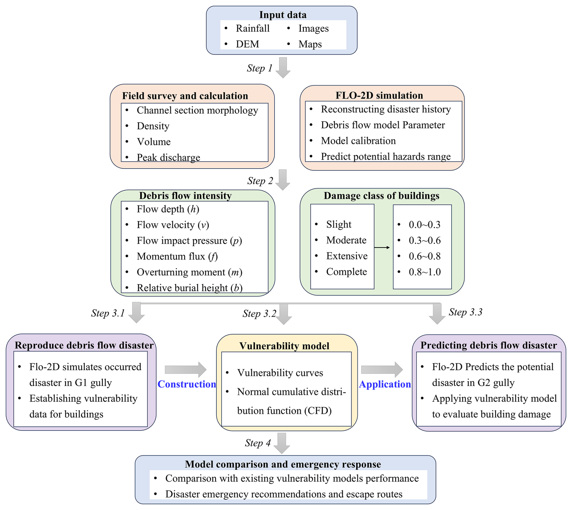
The methodological procedure in this study is divided into four steps (Fig. 1). In step (1), we conducted a field investigation and obtained images of burned areas, channel morphology, grain size distribution, and features of buildings in gullies affected by debris flows (Fig. 4). Then, we calculated the physical characteristic parameters of postfire debris flows. Finally, we reproduced and predicted dynamic runout processes via numerical simulations using the FLO-2D model. In step (2), we employed a numerical model to calculate six indicators of the debris flow intensity (Zhang et al., 2018). Moreover, the damage degree of buildings was classified, and vulnerability index values were assigned on the basis of the degree of damage to buildings (Wang et al., 2024). In step (3), we established building vulnerability curves and a function model using the reconstructed debris flow intensity and building damage information from the G1 gully (after postfire debris flow occurrence). We subsequently applied the vulnerability model to predict potential future scenarios of building damage in the G2 gully (under potential future debris flow scenarios), aiming to assess the compound, bilateral threat that both gullies pose to the downstream Kule Village community. Finally, in step (4), we verified and compared the performance of the proposed vulnerability model with that of previous models and provide suggestions for emergency response and evacuation routes during disasters in Kule village. This methodology facilitates a comprehensive analysis of the potential effects of future postfire debris flow events on buildings within the region, offering valuable insights for formulating disaster management and mitigation strategies.

Figure 1 Methodological framework.

2.1 Field investigation and data acquisition

2.1.1 Study area

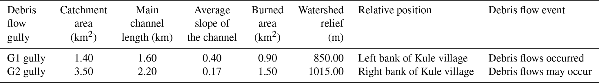
The study area is located in Yajiang County, Sichuan Province, China. Yajiang County occurs in the southeastern part of the Qinghai-Tibet Plateau and the central segment of the Hengduan Mountains within the basin of the Yalong River (He et al., 2024). The Kule watershed (coordinates: 101°4^′12.53^′′ E, 30°7^′55.88^′′ N) is located in the northeastern part of Xiala town in Yajiang County, and the terrain encompasses mainly high mountains and deep canyons. The study area of the Kule watershed contains two primary gullies (G1 and G2), which converge with the main river in the downstream impact area of Kule village (Fig. 2). Kule village contains 58 households with 308 people, and the Kule River flows through the downstream alluvial fan of this village. The left and right banks of the village are impacted by the G1 and G2 gullies, respectively. The catchments of the G1 gully and G2 gully cover areas of 1.4 and 3.5 km², respectively, and the terrain elevation differences range from 850–1015 m. Geologically, the area primarily comprises Late Triassic silty slate. The bedrock is severely weathered and structurally fragmented. Within the catchment, the bedrock is overlain by Quaternary sediments that are approximately 1.0–3.0 m thick (He et al., 2024). The thin residual soil layer is susceptible to failure during periods of intense rainfall.

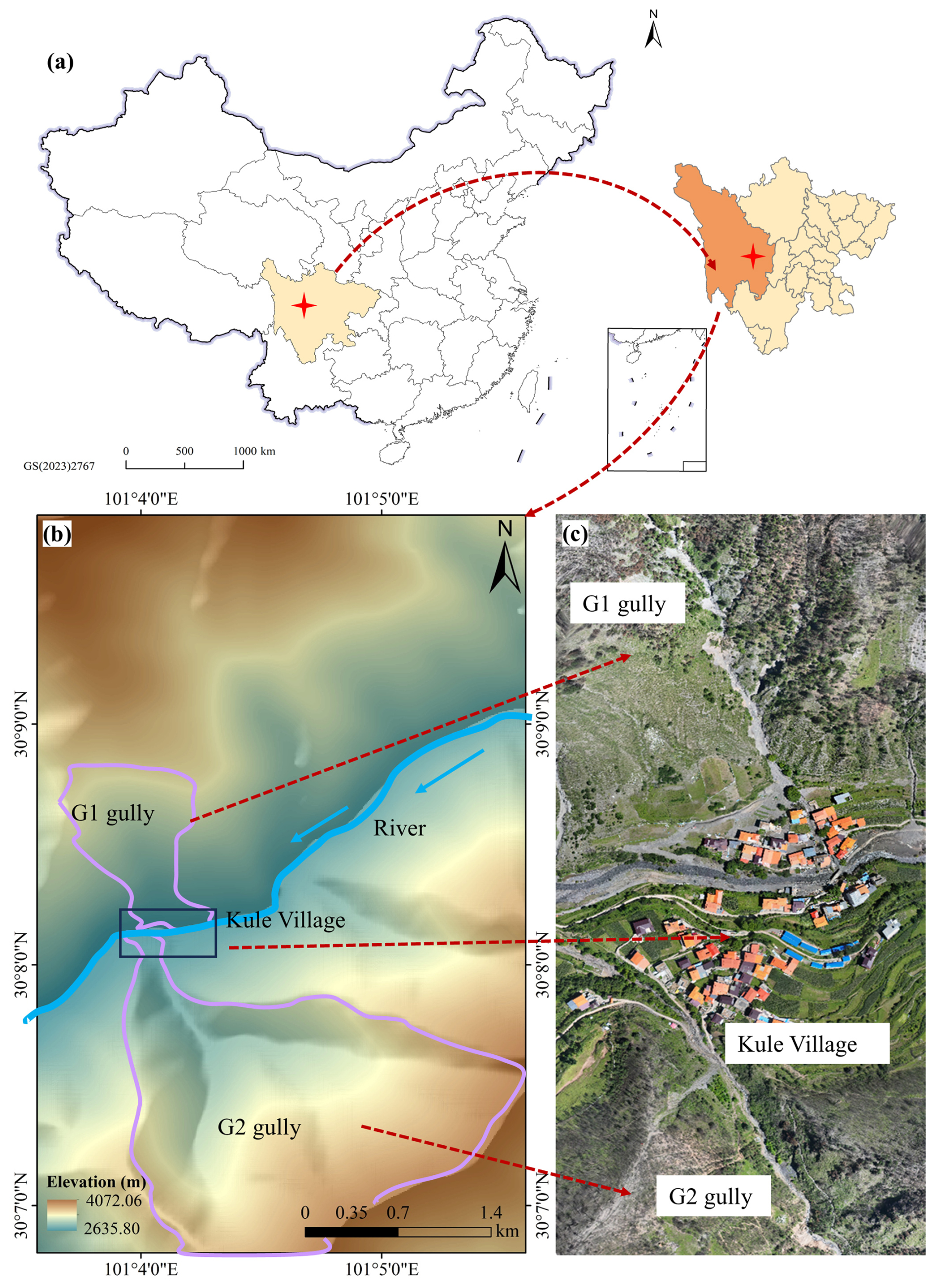
Figure 2 Location of the study area in the Kule Gully, Yajiang County, Sichuan Province, China.

On 15 March 2024, a wildfire ignited in Yajiang County, burning 278.8 km² of mountainous forest and affecting 250 watersheds, with moderate-high burn levels accounting for more than 50 % of the total catchment area (He et al., 2024). Several postfire debris flows occurred in the burned catchments on 10 May that were induced by rainfall events following the fire. In particular, the postfire debris flows in the G1 gully in Kule village destroyed 36 houses, blocked roads, and displaced people. Postfire debris flow and building damage data were collected from this event to support building vulnerability assessment and disaster reduction efforts (Zhang et al., 2018; Gorr et al., 2024).

Yajiang County occurs in a plateau monsoon climate zone, and the long-term annual precipitation ranges from 600 to 1200 mm, with precipitation mainly concentrated from June to September, which accounts for about 86 % of the annual total, with a recent decadal average (2010–2020) of 705 mm. The rainstorm started at 14:00 Beijing time on 10 May and lasted until 11 May, according to records from a rainfall monitoring station (coordinates: 101°1^′20^′′ E, 30°1^′57^′′ N). The maximum recorded hourly rainfall intensity was 6.9 mm h⁻¹, and the accumulated rainfall reached 37.8 mm (Fig. 3). Notably, the rainfall threshold of postfire debris flows is much lower than that of nonfire debris flows (Ouyang et al., 2023). In particular, low-intensity rainfall can trigger postfire debris flows in the G1 gully, and the G2 gully occurs in a state in which debris flows can occur at any time. Owing to wildfires, a large amount of loose material remains on hillslopes and in channels, which can provide abundant material sources for triggering debris flows (McGuire et al., 2024). Thus, debris flow activity in the G1 and G2 gullies may last longer.

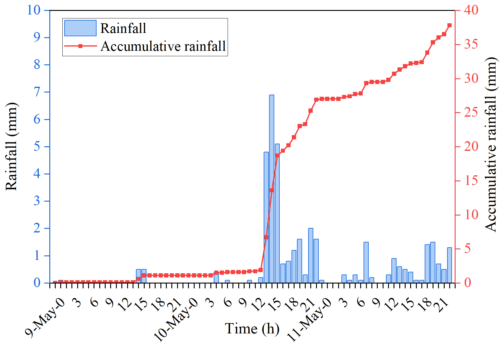
Figure 3 Hydrological characteristics: distributions of the hourly and cumulative rainfall levels.

2.1.2 Field data collection

An unmanned aerial vehicle (UAV) (Inspire3, DJI-Innovations; vertical accuracy: ±0.1 m; horizontal accuracy: ±0.3 m) was employed to obtain images of the G1 and G2 gullies, which were used to acquire topographic and geomorphic information of channels and the spatial distribution of buildings (Fig. 5). A laser rangefinder (Contour XLRic, with a maximum range of 1850 m and a measurement accuracy of 0.10 m) was applied to measure the dimensions of buildings (floor height, width, and length) and the section size of channels (width, gully bed gradient, and bank slope angle) (Fig. 4). The structural type, impact azimuth, affected portion and damage degree of the building were recorded with a camera (SONY A6400). The size of stone blocks, thickness of the ash layer and burned soil, burial height and flow depth mark were measured with a scale. The particle size of postfire debris flows was measured with vibrating sieving machines (measuring range: 0.25–20 mm) and Malvern particle size analysers (measuring range: 0.02–2000 µm; scanning speed: 1000 Hz). Then, the samples were analysed to obtain particle size distribution curve. Derived from sieving and laser analysis, the curve only includes particles up to 20 mm and excludes the larger boulders documented in the field (Fig. 4f). Field work served as the basis for the subsequent simulations and the determination of postfire debris flow physical parameters.

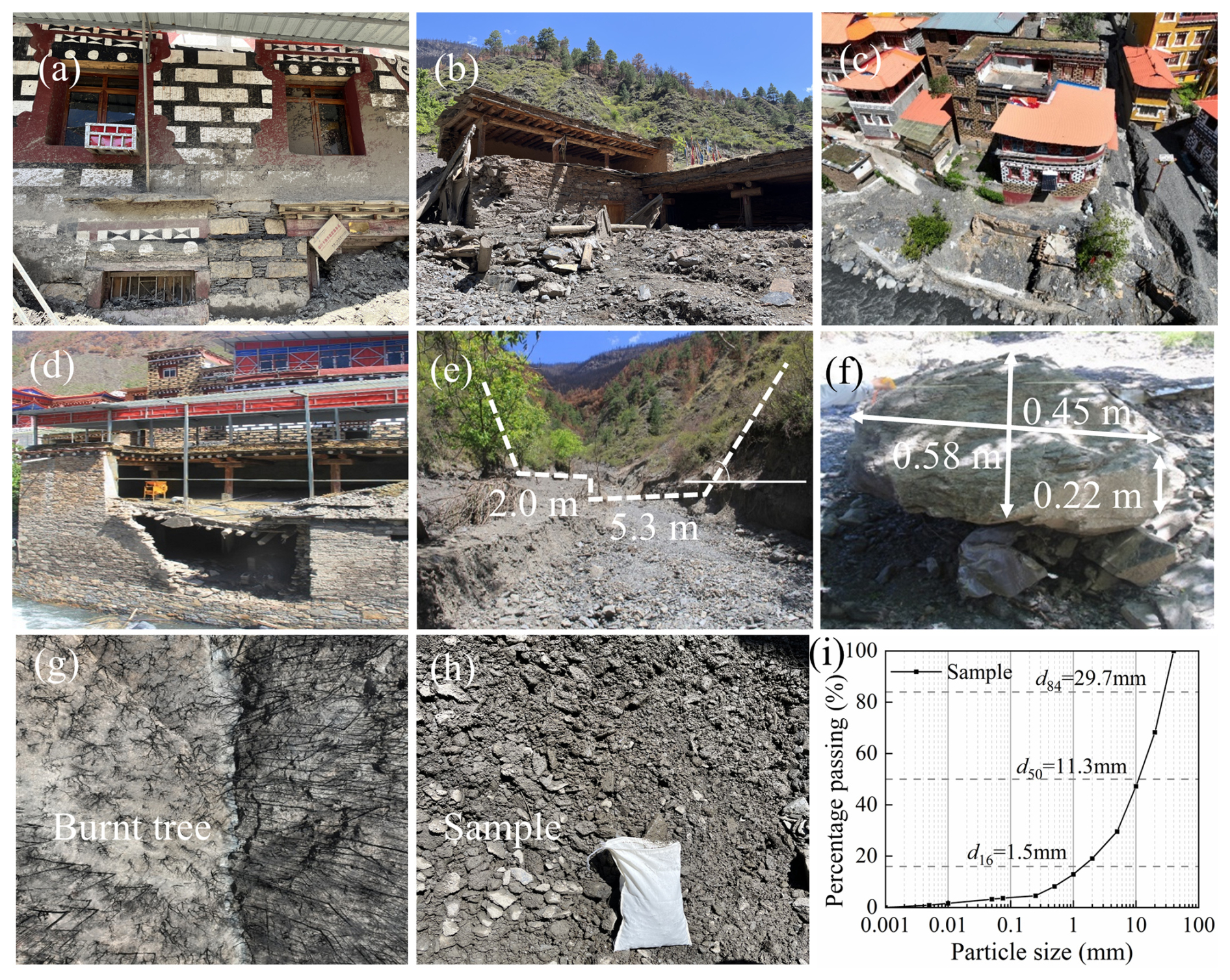
Figure 4 Fieldwork techniques for capturing postfire debris flow events: (a–d) damaged buildings; (e) channel section; (f) block stone size; (g) burned area; (h) particle sampling; (i) particle size distribution curve.

The obtained aerial images were subsequently processed using PhotoScan software to generate a 3D digital orthophoto in the WGS-1984 geographic coordinate system (Wang et al., 2024) and to produce a digital elevation model (DEM), which served as base data for the subsequent runout analyses. These digital model data facilitated the identification of geomorphic features within the G1 and G2 catchments and the spatial distribution of damaged buildings (Fig. 5). The G1 and G2 gullies are located on the left and right banks of Kule village, respectively. G1 and G2 are spatially adjacent and exhibit similarities in terms of geological setting, soil type, vegetation, catchment hydrological characteristics, fire history, and field-observed surface material composition. The catchment area of the G1 gully is small, but the longitudinal gradient of the main channel is steeper with extensive moderate-high burned areas (He et al., 2024). The catchment area of the G2 gully is large, with a gentler longitudinal gradient of the main channel and a larger relative terrain elevation difference. Twelve cross-sectional channel measurements (sections 1 to 12, six per gully) revealed that the channel width gradually increases from upstream to downstream, ranging from 2 to 10 m (Fig. 5). In Fig. 5, “horizontal distance” is lateral distance from the channel center, with zero at the center; “left” and “right” indicate the two banks of the channel. The characteristic parameters of the G1 and G2 gullies are listed in Table 1.

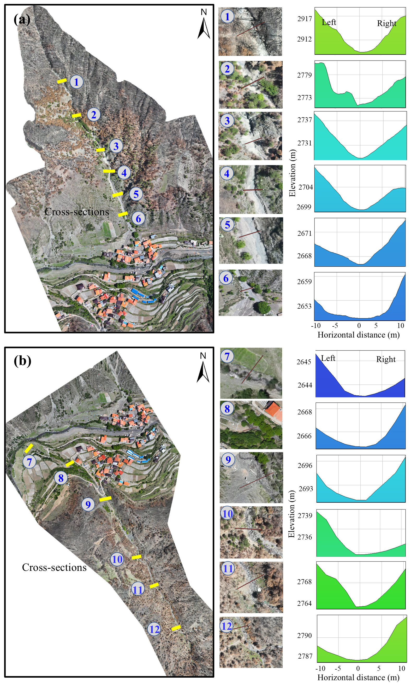
Figure 5 Characteristics of different channel cross sections: (a) G1 debris flow channel on the left bank of Kule village; (b) G2 debris flow channel on the right bank of Kule village.

Table 1 Characteristics of the G1 and G2 gullies on both sides of Kule village, Yajiang County.

2.1.3 Calculation of postfire debris flow parameters

1. Debris flow density

The particle size distribution of a given debris flow deposit can be used to determine the debris flow density, which can be calculated as follows (Wang et al., 2024; Chen et al., 2021):

$$\begin{array}{}\text{(1)}& {\mathit{\gamma }}_{\mathrm{d}}={\mathit{\gamma }}_{\mathrm{0}}+{\mathit{\gamma }}_{\mathrm{m}}{P}_{\mathrm{2}}(P_{\mathrm{0.05}}{)}^{\mathrm{0.35}}\end{array}$$

where γ_d is the density of the debris flow (t m⁻³); γ_m is the minimum density of a viscous debris flow (2.0 t m⁻³); γ₀ is the minimum density of the debris flow (1.4–1.5 t m⁻³); P₂ is the percentage of coarse particles with a diameter greater than 2 mm; and P_0.05 is the percentage of fine particles with a diameter smaller than 0.05 mm (Table 2).

Table 2 Key input parameters coefficient for debris flow calculations.

2. Debris flow volume

The US Geological Survey (USGS) debris flow hazard assessment system is based on a model developed by Gartner et al. (2014) for estimating the volume of postfire debris flows. The emergency assessment volume model is a multiple linear regression model and has been widely applied (Rengers et al., 2023; Gorr et al., 2024). This model can be expressed as follows:

$$\begin{array}{}\text{(2)}& \ln \left(V_{\mathrm{DF}}\right)=\mathrm{4.22}+\mathrm{0.39}\sqrt{I_{\mathrm{15}}}+\mathrm{0.36}\ln \left(B_{\mathrm{mh}}\right)+\mathrm{0.13}\sqrt{R}\end{array}$$

where V_DF is the postfire debris flow volume (m³); I₁₅ is the 15 min maximum rainfall intensity (mm h⁻¹); B_mh is the burned area with moderate and high burn severity levels (km²); and R is the watershed relief (m).

3. Debris flow peak discharge

The debris flow peak discharge can be estimated via the volume-peak discharge relationship method (Rickenmann 1999; Marchi et al., 2002) or the rain-flood method (Zhou et al., 1991; Cui et al., 2023).

First, the peak discharge for a given catchment can be estimated on the basis of the debris flow volume (Kang and Kim, 2016). Notably, studies have demonstrated that the debris flow volume is related to the peak discharge (Navratil et al., 2013; Cui et al., 2018; Guo et al., 2024):

$$\begin{array}{}\text{(3)}& Q_{\mathrm{d}}=\mathit{\alpha }{V}_{\mathrm{DF}}^{\mathit{\beta }}\end{array}$$

where Q_d is the peak discharge of the debris flow (m³ s⁻¹); V_DF is the postfire debris flow volume (m³), which can be calculated by Eq. (2); and α and β are fitting coefficients for different watersheds, with a specific range. Please refer to Guo et al. (2024) for further details.

Second, the rain-flood method can be used for calculating rainfall-triggered debris flows under different rainfall frequency conditions (Zhou et al., 1991; Chang et al., 2020):

$$\begin{array}{}\text{(4a)}& Q_{\mathrm{d}}=\left(\mathrm{1}+\mathit{\varphi }\right)Q_{\mathrm{f}}{D}_u\end{array}$$

where Q_f is the peak flood discharge of clean water (m³ s⁻¹); Q_d is the peak flow of the debris flow (m³ s⁻¹); D_u is the blockage amplification factor; ϕ is the solids concentration, ϕ = $\left({\mathit{\gamma }}_{\mathrm{d}}-\mathrm{1})/({\mathit{\gamma }}_{\mathrm{s}}-{\mathit{\gamma }}_{\mathrm{d}}\right)$; and γ_d and γ_s are the densities of the debris flow and solid materials (t m⁻³), respectively.

$$\begin{array}{}\text{(4b)}& Q_{\mathrm{f}}=\mathrm{0.278}\mathit{\phi }{\displaystyle \frac{S}{{\mathit{\tau }}^n}}F\end{array}$$

where φ is the peak runoff coefficient; S is the storm force (mm h⁻¹), namely, the maximum 1 h rainstorm intensity; τ is the confluence time (h); n is the rainstorm attenuation index; and F is the watershed area (km²). The parameters in Eq. (4b) can be obtained by consulting the calculation manual and can be calculated as follows (Sichuan Hydrological Manual, 1984; Cui et al., 2023):

$$\begin{array}{}\text{(5a)}& {\displaystyle }\mathit{\phi }=\mathrm{1}-\mathrm{1.1}{\displaystyle \frac{\mathit{\mu }}{S}}{t}_{\mathrm{0}}^n\text{(5b)}& {\displaystyle }S=H_{\mathrm{1}}{K}_{\mathrm{1}}\text{(5c)}& {\displaystyle }t=t_{\mathrm{0}}{\mathit{\phi }}^{-\frac{\mathrm{1}}{\mathrm{4}-n}}\text{(5d)}& {\displaystyle }n=\mathrm{1}+\mathrm{1.285}\left(\text{lg}{\displaystyle \frac{H_{\mathrm{1}}{K}_{\mathrm{1}}}{H_{\mathrm{6}}{K}_{\mathrm{6}}}}\right)\text{(5e)}& {\displaystyle }\mathit{\mu }=\mathrm{3.6}{K}_p{F}^{-\mathrm{0.19}}\text{(5f)}& {\displaystyle }{t}_{\mathrm{0}}={\left({\displaystyle \frac{\mathrm{0.383}}{m{S}^{\mathrm{1}/\mathrm{4}}/\mathit{\theta }}}\right)}^{\frac{\mathrm{4}}{\mathrm{4}-n}}\text{(5g)}& {\displaystyle }m=\mathrm{0.221}{\mathit{\theta }}^{\mathrm{0.204}}\text{(5h)}& {\displaystyle }\mathit{\theta }={\displaystyle \frac{L}{J^{\mathrm{1}/\mathrm{3}}{F}^{\mathrm{1}/\mathrm{4}}}}\end{array}$$

where μ is the current generation parameter (mm h⁻¹); t₀ is the confluence time of the basin; H₁ and H₆ are the 1 and 6 h average rainfall amounts, respectively (mm); K₁ and K₆ are the modulus coefficients corresponding to periods H₁ and H₆, respectively; K_p is the modulus ratio coefficient of the Pearson curve; m is the confluence parameter; θ is the watershed coefficient; J is the slope of the channel; and L is the main channel length (km).

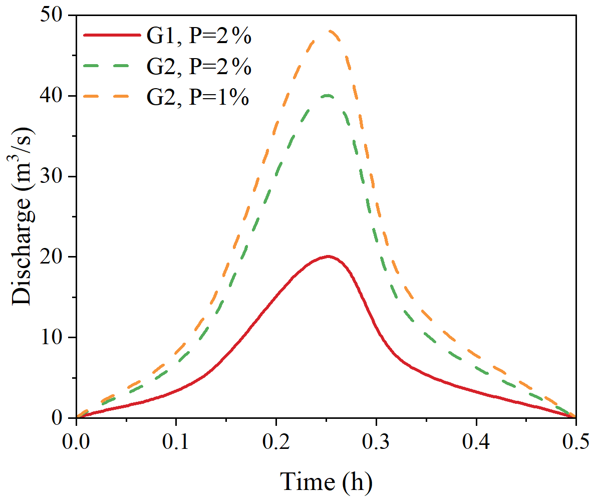
Finally, we combined the results of the two peak discharge calculation methods to determine the peak discharges of the postfire debris flows in the G1 and G2 gullies at different frequencies (Fig. 6). The flow process line of debris flow discharge can be obtained by using the generalized pentagon method, which has been widely adopted in previous studies (Zhang et al., 2023; Ding et al., 2023).

Figure 6 Flow hydrographs of the G1 and G2 gullies at different frequencies.

2.2 FLO-2D numerical simulation of disaster scenarios

2.2.1 Governing equations for rainfall runoff and debris flows

The two-dimensional numerical debris flow evolution model FLO-2D was applied to simulate the runout process and to quantify key metrics of debris flows in the G1 and G2 gullies (Wang et al., 2024; Si et al., 2022; Zhang et al., 2018; Chang et al., 2020). On the basis of 2D shallow water equations, mass and momentum conservation equations are employed in the FLO-2D model as the governing equations:

$$\begin{array}{}\text{(6a)}& {\displaystyle }i={\displaystyle \frac{\partial h}{\partial t}}+{\displaystyle \frac{\partial h\partial V_x}{\partial x}}+{\displaystyle \frac{\partial h\partial V_y}{\partial y}}\text{(6b)}& {\displaystyle }{S}_{fx}=S_{ox}-{\displaystyle \frac{\partial h}{\partial x}}-{\displaystyle \frac{V_x}{g}}{\displaystyle \frac{\partial V_x}{\partial x}}-{\displaystyle \frac{V_y}{g}}{\displaystyle \frac{\partial V_x}{\partial y}}-{\displaystyle \frac{\mathrm{1}}{g}}{\displaystyle \frac{\partial V_x}{\partial t}}\text{(6c)}& {\displaystyle }{S}_{fy}=S_{oy}-{\displaystyle \frac{\partial h}{\partial y}}-{\displaystyle \frac{V_y}{g}}{\displaystyle \frac{\partial V_y}{\partial y}}-{\displaystyle \frac{V_x}{g}}{\displaystyle \frac{\partial V_y}{\partial x}}-{\displaystyle \frac{\mathrm{1}}{g}}{\displaystyle \frac{\partial V_y}{\partial t}}\end{array}$$

where h is the flow depth; V_x and V_y are the depth-averaged velocities along the horizontal x and y coordinates, respectively; i is the intensity at the flow surface; and S_fx and S_fy are the friction slopes, expressed as functions of bed slopes S_ox and S_oy, respectively, the pressure gradient and the convective and local acceleration terms (Chen et al., 2021). The total friction slope, S_f, is the sum of the yield slope, the viscous slope, and the turbulent dispersive slope (Zhang et al., 2018), which can be obtained as follows:

$$\begin{array}{}\text{(7)}& S_f={\displaystyle \frac{{\mathit{\tau }}_y}{{\mathit{\gamma }}_{m}h}}+{\displaystyle \frac{K\mathit{\eta }v}{\mathrm{8}{\mathit{\gamma }}_m{h}^{\mathrm{2}}}}+{\displaystyle \frac{n^{\mathrm{2}}{v}^{\mathrm{2}}}{h^{\mathrm{4}/\mathrm{3}}}}\end{array}$$

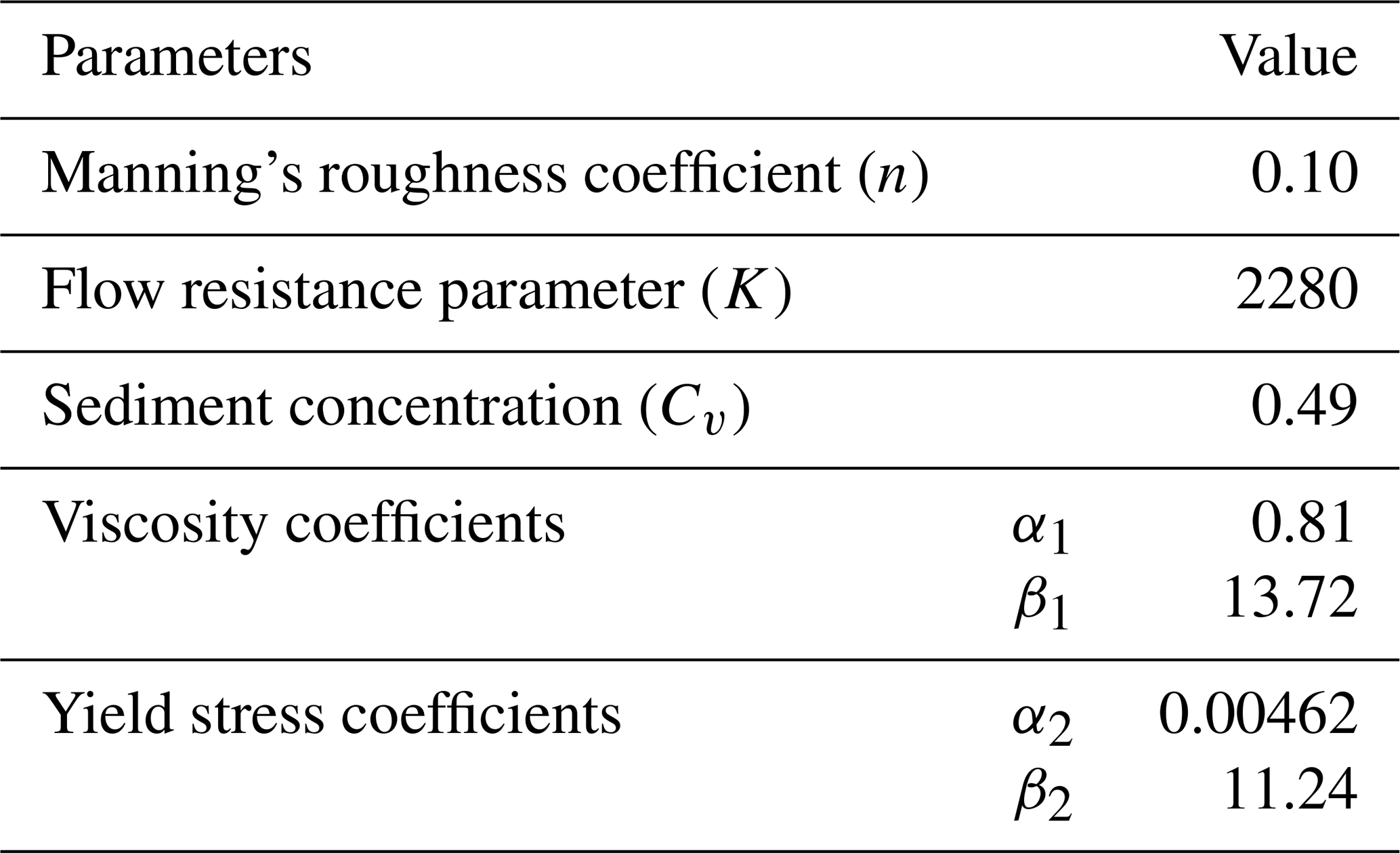
where n is Manning's coefficient; K is flow resistance parameter; η is the dynamic viscosity (Pa s⁻¹), and τ_y is the yield stress (Pa), which can be calculated as follows:

$$\begin{array}{}\text{(8a)}& {\displaystyle }\mathit{\eta }={\mathit{\alpha }}_{\mathrm{1}}{e}^{{\mathit{\beta }}_{\mathrm{1}}{C}_v}\text{(8b)}& {\displaystyle }{\mathit{\tau }}_y={\mathit{\alpha }}_{\mathrm{2}}{e}^{{\mathit{\beta }}_{\mathrm{2}}{C}_v}\end{array}$$

where C_v is the sediment concentration, and α₁, α₂, β₁, and β₂ are empirical coefficients.

The FLO-2D simulations were conducted by adding elevation data of the computation area to the grid, which was set to 5 m × 5 m, after which the inlet and outlet conditions, the rheological parameters (Table 3), the duration of the debris inflow hydrograph (i.e., 30 min) and the peak discharge were defined. Manning's roughness coefficient of 0.1 is selected referring to the FLO-2D manual, and the same value adopted in previous studies (Zhang et al., 2018; Chen et al., 2021). Finally, the dynamics and key parameters, such as the flow depth and flow velocity, were obtained.

Table 3 The rheological parameters for the debris flow simulation.

2.2.2 Model calibration and validation

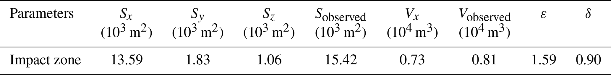
To ensure accuracy, the methodology proposed by Scheidl and Rickenmann (2010) was adopted to validate the simulation results (Table 4). We measured the observed depositional fan area through field investigations and the predicted depositional fan area obtained with the FLO-2D model (Chen et al., 2021). The subareas (X, Y and Z) were obtained via the overlay of the predicted deposition area with the observed deposition area. We assessed the overall reconstruction accuracy via the following evaluation parameters (Chen et al., 2021; Wang et al., 2024):

$$\begin{array}{}\text{(9)}& {\displaystyle }\mathit{\epsilon }={\displaystyle \frac{S_X}{S_{\mathrm{observed}}}}-{\displaystyle \frac{S_Y}{S_{\mathrm{observed}}}}-{\displaystyle \frac{S_Z}{S_{\mathrm{observed}}}}+{\displaystyle \frac{V_X}{V_{\mathrm{observed}}}}\text{(10)}& {\displaystyle }\mathit{\delta }=frac\mathit{\epsilon }+\mathrm{24}\end{array}$$

where S_X, S_Y, and S_Z are the positive accuracy region, negative accuracy region, and missing accuracy region, respectively; S_observed is the actual impact zone; V_X is the correct judgement volume; V_observed is the actual volume; and δ is the normalized accuracy value, with values ranging from 0 to 1.

Table 4 Calibration parameters and accuracy of the numerical simulation results.

2.3 Development of empirical vulnerability models for buildings

2.3.1 Damage class of buildings

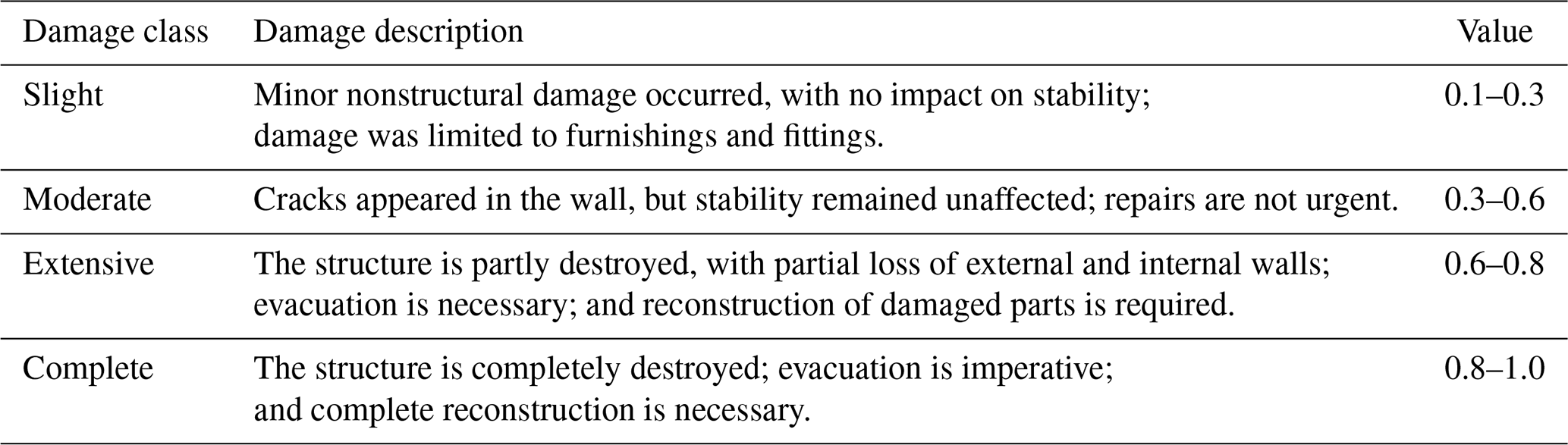
Kule village encompasses a total of 128 buildings, with 36 buildings on the left bank affected by postfire debris flows in the G1 gully. The damage to buildings notably depends on their structural type, material resistance and distribution density (Zhang et al., 2018). In the study area, 95 % of the affected main building structures are BC structural-type buildings, which are widely distributed in mountainous areas across China (Chen et al., 2021). We subsequently aimed to develop vulnerability curves for BC buildings. Most buildings in the study area comprise 1–3 floors, and the building height ranges from 3–8 m. To determine the degree of damage to buildings caused by debris flows, it is necessary to establish a classification standard on the basis of the actual structural and damage degree conditions (Hu et al., 2012; Lee et al., 2024). Table 5 provides the four categories of damage to a given structure and the corresponding vulnerability index values, including slight, moderate, extensive, and complete damage. On the basis of the above assumptions and analysis, damaged buildings affected by debris flows in Kule village were constructed (Appendix A).

Table 5 Damage classes and definitions for buildings (Hu et al., 2012; Wang et al., 2024; Lee et al., 2024).

2.3.2 Debris flow intensity

In this study, six commonly used debris flow intensities were selected as multidimensional indicators of the destruction potential (Quan Luna et al., 2011; Eidsvig et al., 2014; Kang and Kim, 2016; Zhang et al., 2018; Chen et al., 2021; Wang et al., 2024; Lee et al., 2024), including the flow depth (h), flow velocity (v), impact pressure (p), momentum flux (f), overturning moment (m), and relative burial height (b).

The flow impact pressure includes both hydrostatic and hydrodynamic forces (Kang and Kim, 2016; Wang et al., 2024), and the total impact pressure exerted by a debris flow can be expressed as:

$$\begin{array}{}\text{(11)}& p={\displaystyle \frac{\mathrm{1}}{\mathrm{2}}}\mathit{\rho }gh+\mathit{\rho }{v}^{\mathrm{2}}\end{array}$$

where p is the impact pressure (Pa); v is the flow velocity (m s⁻¹); and h is the flow depth (m), ρ is the debris flow density (kg m⁻³).

The momentum flux can be obtained by multiplying the flow depth and the square of the flow velocity (Jakob et al., 2012; Chen et al., 2021):

$$\begin{array}{}\text{(12)}& f=h{v}^{\mathrm{2}}\end{array}$$

where f is the momentum flux (m³ s⁻²).

The overturning moment of a debris flow is related to the maximum flow velocity and depth at which it collides with a given structure, as reported by Zhang et al. (2018):

$$\begin{array}{}\text{(13)}& m=vh\end{array}$$

where m is the overturning moment (m² s⁻¹).

The relative burial height is defined by the deposition height and the affected building height to represent the degree of burial damage (Totschnig et al., 2011; Zhang et al., 2018):

$$\begin{array}{}\text{(14)}& b={\displaystyle \frac{h_{\mathrm{d}}}{h_{\mathrm{b}}}}\end{array}$$

where b is the relative burial height, h_d is the deposition height (m), and h_b is the building height (m).

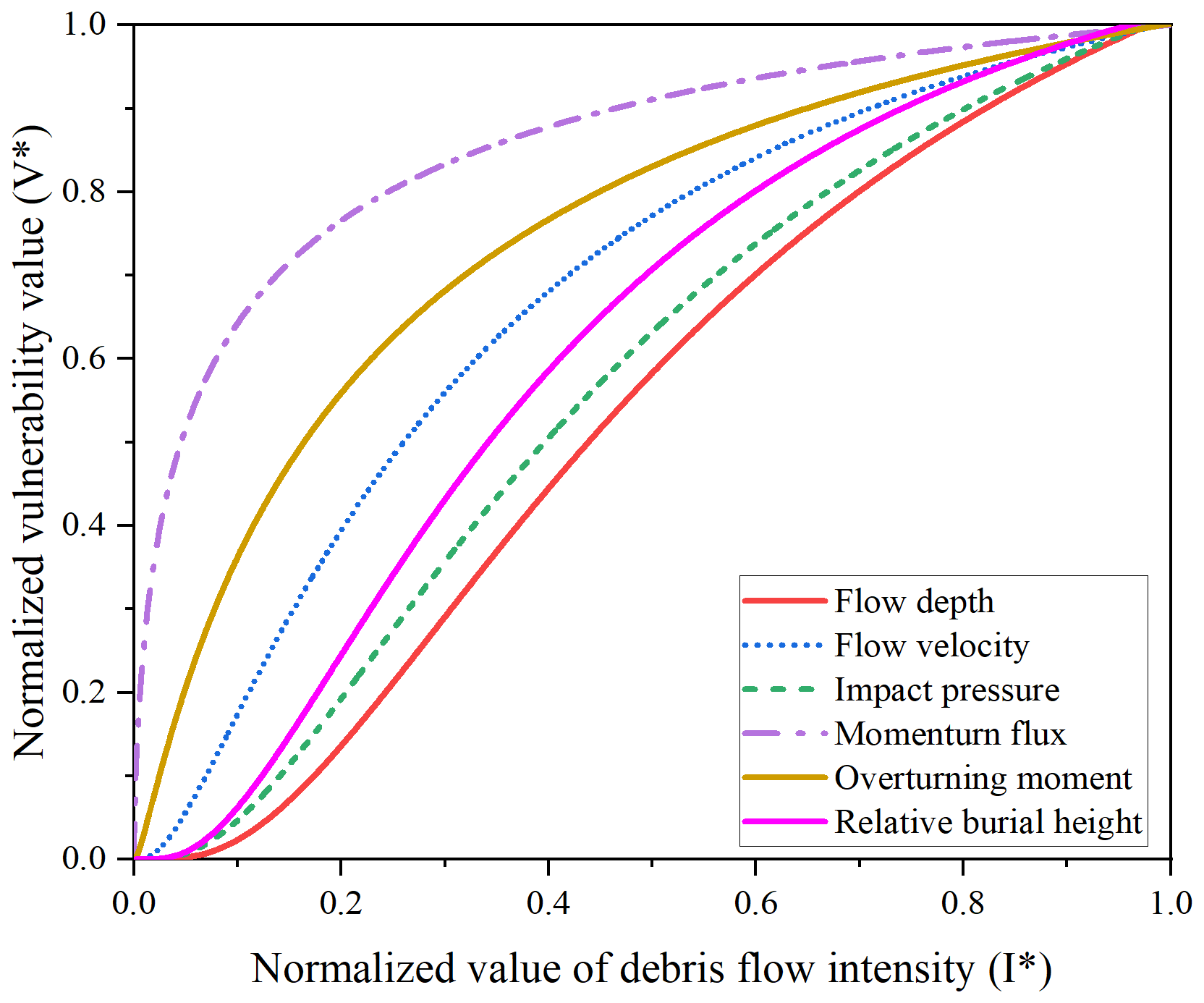
Under the same damage state, vulnerability values derived from different intensity indicators may vary, potentially leading to inconsistent damage classification (Luo et al., 2023). To enable a direct comparison of indicator performance in Sect. 4.1 (note that normalized values are used exclusively for the analysis in that section), both intensity and vulnerability values were normalized using the following equations (Zhang et al., 2024):

$$\begin{array}{}\text{(15a)}& {\displaystyle }{I}^{\ast }={\displaystyle \frac{I-min\left(I\right)}{max\left(I\right)-min\left(I\right)}}\text{(15b)}& {\displaystyle }{V}^{\ast }={\displaystyle \frac{V-min\left(V\right)}{max\left(V\right)-min\left(V\right)}}\end{array}$$

where I^∗ and V^∗ are the normalized values of the debris flow intensity and vulnerability, respectively.

2.3.3 Vulnerability curve

The vulnerability model captures the relationship between the probability of building damage reaching a certain state and the debris flow intensity (Cui et al., 2011). Notably, postdisaster data-driven vulnerability curves can be expressed via function models (Fuchs et al., 2019). Currently, many vulnerability functions, such as logistic, Weibull, exponential, power-law and Avrami functions, are employed (Quan Luna et al., 2011; Eidsvig et al., 2014; Chen et al., 2021; Lee et al., 2024). However, the uncertainties in these models originate from the curve fitting process. For example, the use of the exponential function cannot guarantee that the curve passes through the origin. Therefore, recent studies have indicated that lognormal cumulative distribution function (LNCDF) vulnerability curves provide better performance (Luo et al., 2023):

$$\begin{array}{}\text{(16)}& V=\mathrm{\Phi }\left[{\displaystyle \frac{\mathrm{1}}{\mathit{\beta }}}\ln \left({\displaystyle \frac{I}{I_{\mathrm{m}}}}\right)\right]\end{array}$$

where β is the standard deviation of the logarithm of the hazard intensity; I is the debris flow hazard intensity; I_m is the median hazard intensity; V is vulnerability value (0–1); and Φ is the LNCDF, which can be expressed as follows:

$$\begin{array}{}\text{(17)}& \mathrm{\Phi }\left(x\right)={\int }_{\mathrm{0}}^x{\displaystyle \frac{\mathrm{1}}{\sqrt{\mathrm{2}\mathit{\pi }}\mathit{\sigma }t}}{e}^{-\frac{{\left(\ln \left(t\right)-\mathit{\mu }\right)}^{\mathrm{2}}}{\mathrm{2}{\mathit{\sigma }}^{\mathrm{2}}}}\mathrm{d}t\end{array}$$

where μ is the mean of the LNCDF, and σ is the standard deviation of the LNCDF.

The performance of models was comparatively analysed via four dimensionless performance indices, namely, the coefficient of determination (R²), the mean relative error (MRE), the Theil inequality coefficient (TIC), and the prediction accuracy factor (PAF). Notably, lower MRE and TIC values reflect higher model performance. Additionally, the closer the PAF value is to 1, the better the agreement between the calculated and experimental values (the higher the prediction accuracy). These indices can be calculated as follows (Lee et al., 2024; Wang et al., 2018):

$$\begin{array}{}\text{(18)}& {\displaystyle }{R}^{\mathrm{2}}=\mathrm{1}-{\displaystyle \frac{{\sum }_{i=\mathrm{1}}^N{\left(I_{\mathrm{cal},i}-I_{\mathrm{obs},i}\right)}^{\mathrm{2}}}{{\sum }_{i=\mathrm{1}}^N{\left(I_{\mathrm{cal},i}-{\stackrel{\mathrm{‾}}{I}}_{\mathrm{obs},i}\right)}^{\mathrm{2}}}}\text{(19)}& {\displaystyle }\text{MRE}={\displaystyle \frac{\mathrm{1}}{N}}{\sum }_{i=\mathrm{1}}^N{\displaystyle \frac{\left|I_{\mathrm{cal},i}-I_{\mathrm{obs},i}\right|}{I_{\mathrm{obs},i}}}\text{(20)}& {\displaystyle }\text{TIC}={\displaystyle \frac{\sqrt{\left({\sum }_{i=\mathrm{1}}^N{\left(I_{\mathrm{cal},i}-I_{\mathrm{obs},i}\right)}^{\mathrm{2}}\right)/N}}{\sqrt{\left({\sum }_{i=\mathrm{1}}^N{I}_{\mathrm{cal},i}^{\mathrm{2}}\right)/N}+\sqrt{\left({\sum }_{i=\mathrm{1}}^N{I}_{\mathrm{obs},i}^{\mathrm{2}}\right)/N}}}\text{(21)}& {\displaystyle }\text{PAF}={\mathrm{10}}^{\frac{{\sum }_{i=\mathrm{1}}^N\log \left|I_{\mathrm{cal},i}/I_{\mathrm{obs},i}\right|}{N}}\end{array}$$

where N is the total number of data points, and I_cal,i and I_obs,i are the calculated and observed values of case i, respectively.

3 Results

3.1 Reproduction of the debris flow intensity and building damage in the G1 gully

Figure 7a shows the characteristics of the degree of damage to buildings and the distribution of buildings in the G1 gully. There are 36 buildings on the left bank of Kule village affected by postfire debris flows in the G1 gully. Notably, the numbers of buildings with slight, moderate, extensive and complete damage are 8, 7, 9 and 12, respectively. Figure 7b shows that the FLO-2D simulations reproduce the runout process of debris flows in the G1 gully that occurred on 10 May 2024, and distribution maps of the inundation area, flow velocity and flow depth were obtained. The buildings were impacted and buried by debris flows, the flow depth near the impacted buildings ranged from 0.25 to 2.61 m, and the flow velocity near the buildings ranged from 0.04 to 1.93 m s⁻¹. This occurred because the debris flow energy partly dissipates under the influence of building groups, and sediment is deposited inside the buildings. The debris flow also partially entered the main river, causing blockages at bridges connecting the villages on both sides (Fig. 7c).

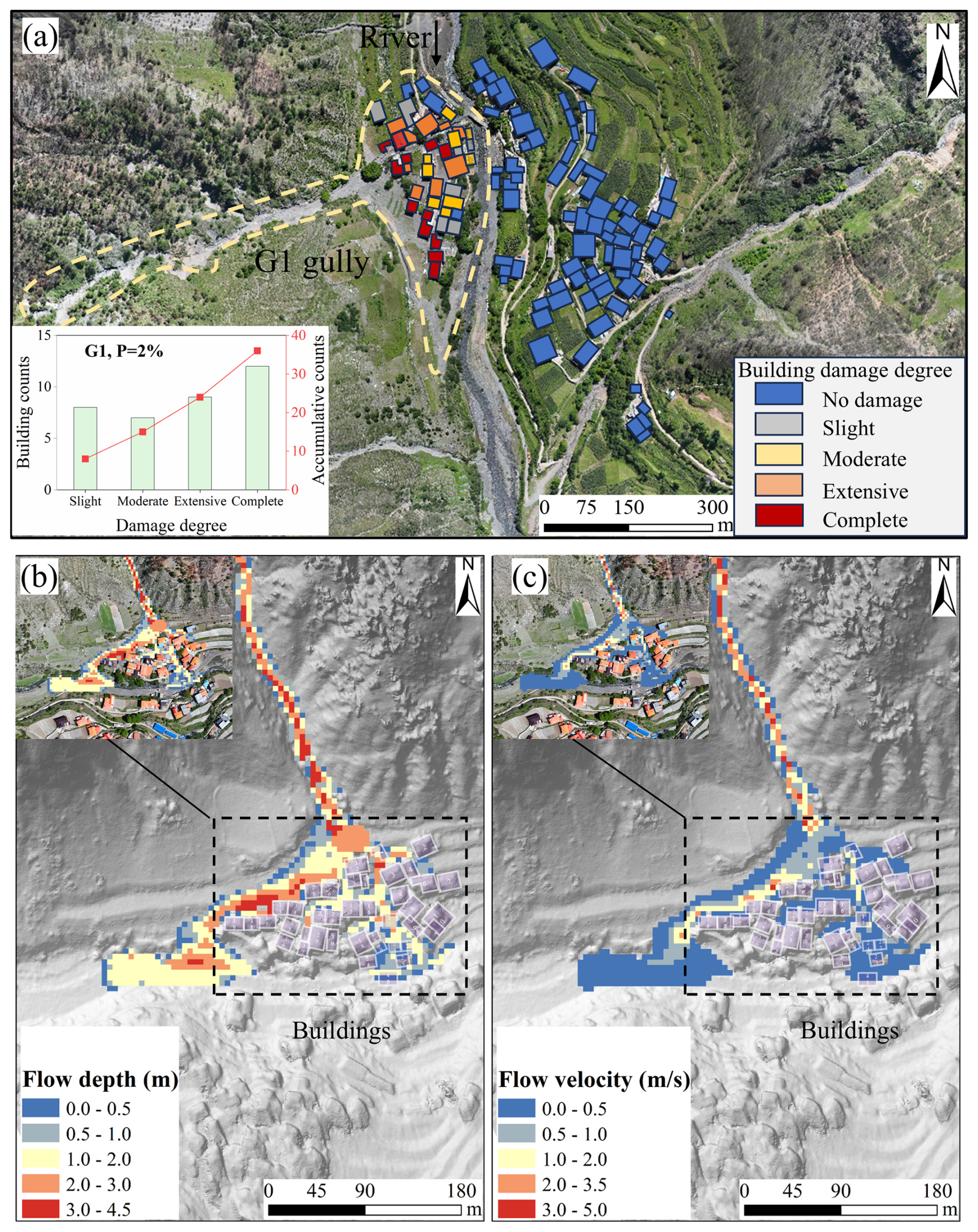
Figure 7 Building damage from field survey and debris flow reconstruction using FLO-2D in the G1 gully: (a) distribution and statistics of building damage; (b) flow depth map; (c) flow velocity map.

3.2 Development of the vulnerability model

Figure 8 shows six groups of developed vulnerability curves for the 2024 postfire debris flow events in the G1 gully, including the flow depth, flow velocity, impact pressure, momentum flux, overturning moment and relative burial height. The vulnerability curve can be obtained via a continuum function relating the debris flow intensity (X axis) to the degree of building damage (Y axis). The LNCDF effectively described the trend in the data. Each vulnerability curve is a monotonically increasing function, indicating that with increasing debris flow intensity, the probability of failure gradually increases. When the slope of the vulnerability curve suddenly increases, the ability of the structure to resist disasters rapidly decreases after critical-strength debris flow disaster occurrence, leading to a rapid increase in the probability of failure. Specifically, to reach a maximum vulnerability value of 1, BC buildings necessitate a flow depth greater than 6 m, a flow velocity of 5 m s⁻¹, an impact pressure of 50 kPa, a momentum flux of 50 m³ s⁻², and an overturning moment of 40 m² s⁻¹. However, completely damaged buildings (with a vulnerability value exceeding 0.8) can no longer function properly. Thus, the critical value of failure is lower, corresponding to a flow depth of 2.5 m, a flow velocity of 1.3 m s⁻¹, an impact pressure of 25 kPa and a relative burial height of 0.48. Additionally, the responses of the various indicators to vulnerability differed, and these differences are analysed in greater detail in the subsequent chapter.

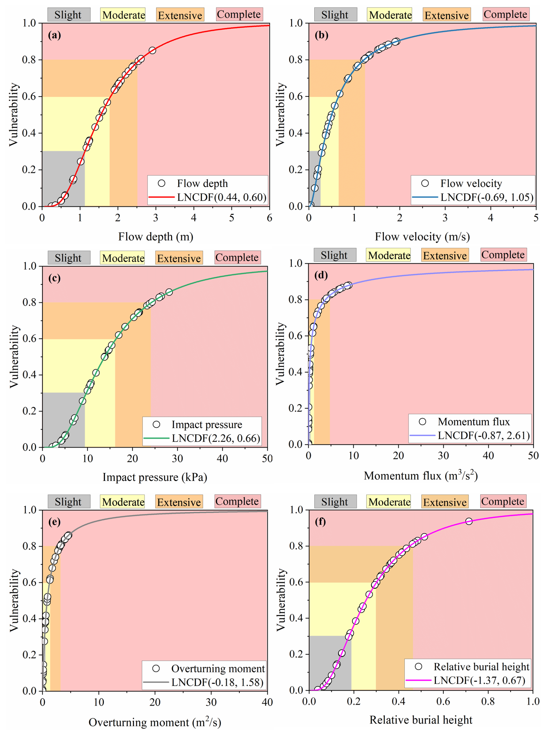
Figure 8 Vulnerability curves for debris flow intensities: (a) flow depth, (b) flow velocity, (c) impact pressure, (d) momentum flux, (e) overturning moment, and (f) relative burial height. The legend “LNCDF (μ, σ)” denotes the lognormal cumulative distribution function (LNCDF), where μ is the mean and σ is the standard deviation for each curve.

3.3 Application of the vulnerability model in the G2 gully

Potential postfire debris flow events may occur in the G2 gully, thus posing a serious threat to buildings on the right bank of Kule village. Figure 9 shows the prediction of potential debris flows in the G2 gully using the FLO-2D model under reproduction frequency conditions of P = 2 % (the peak flow is 40 m³ s⁻¹) and P = 1 % (the peak flow is 48 m³ s⁻¹). The simulated scenarios revealed that the buildings near the channel were significantly affected by the debris flow, and the debris flow flowed into the main river, causing deposition and blockage. The maximum flow depth and flow velocity around the buildings are 3.50 m and 2.36 m s⁻¹, respectively. A comparison of the flow depths between the two recurrence periods revealed that the maximum value under P = 1 % surpassed that under P = 2 by 20 %.

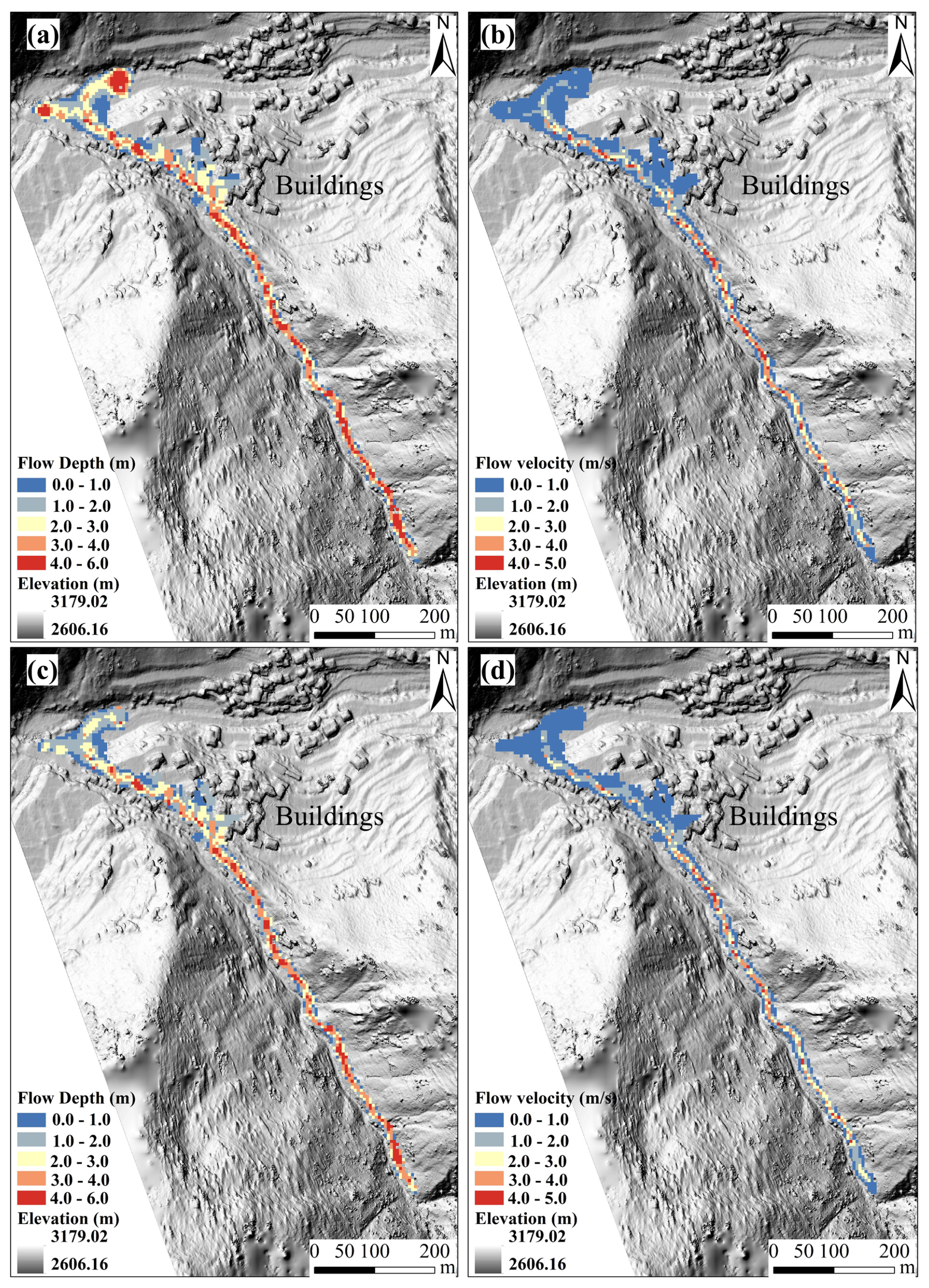
Figure 9 Prediction of the potential debris flow in the G2 gully using the FLO-2D model: (a) flow depth, P = 2 %; (b) flow velocity, P = 2 %; (c) flow depth, P = 1 %; (d) flow velocity, P=2 %.

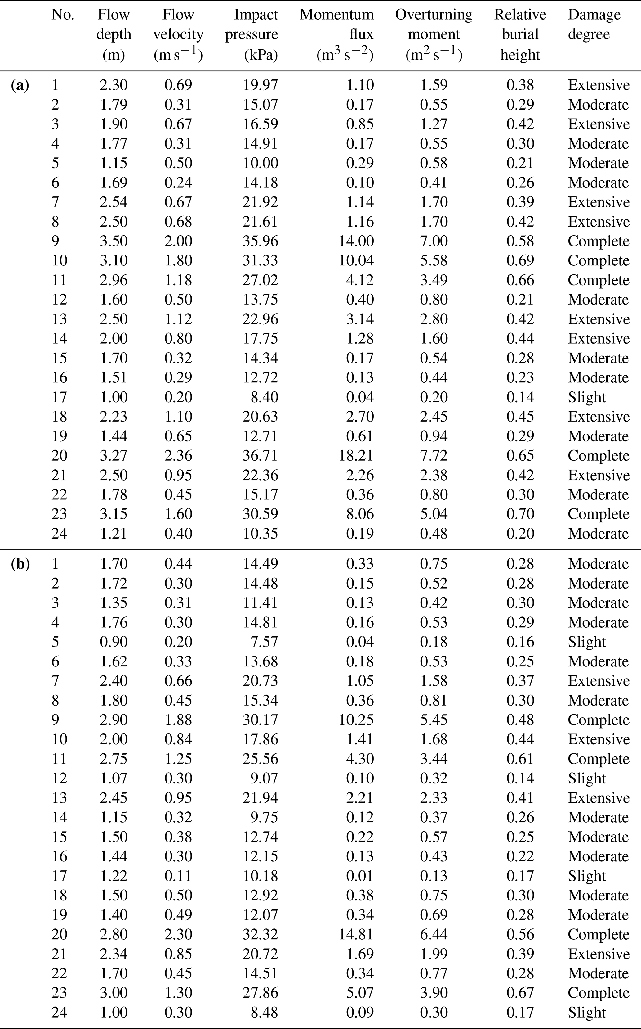
Then, by applying the established vulnerability model to the debris flow intensity data of the G2 gully (Fig. 10), the vulnerability value of damaged buildings in the G2 gully can be calculated from the generated curves (Appendix B). Next, four categories were determined through a combination of vulnerability values and the damage classification system. Figure 11 shows the predicted building damage degree and the spatial distribution under different recurrence periods. The predicted total number of affected buildings is 24, and the numbers of buildings with slight, moderate, extensive and complete damage are 4, 12, 4 and 4, respectively, for P = 2 %. Concurrently, the numbers of buildings with extensive and complete damage exhibit a corresponding uptick under longer recurrence periods (Fig. 12).

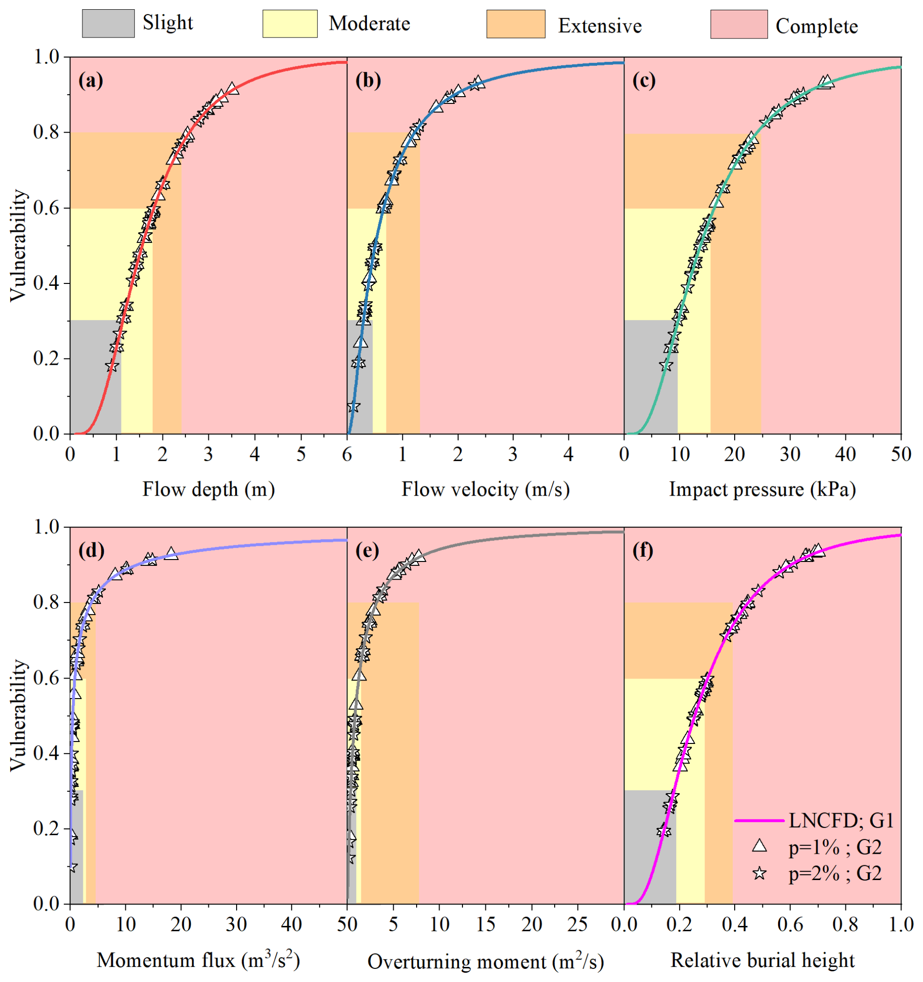
Figure 10 Vulnerability curves for different intensities of debris flows in the G2 gully according to the established vulnerability model for determining the building damage status: (a) flow depth, (b) flow velocity, (c) impact pressure, (d) momentum flux, (e) overturning moment, and (f) relative burial height.

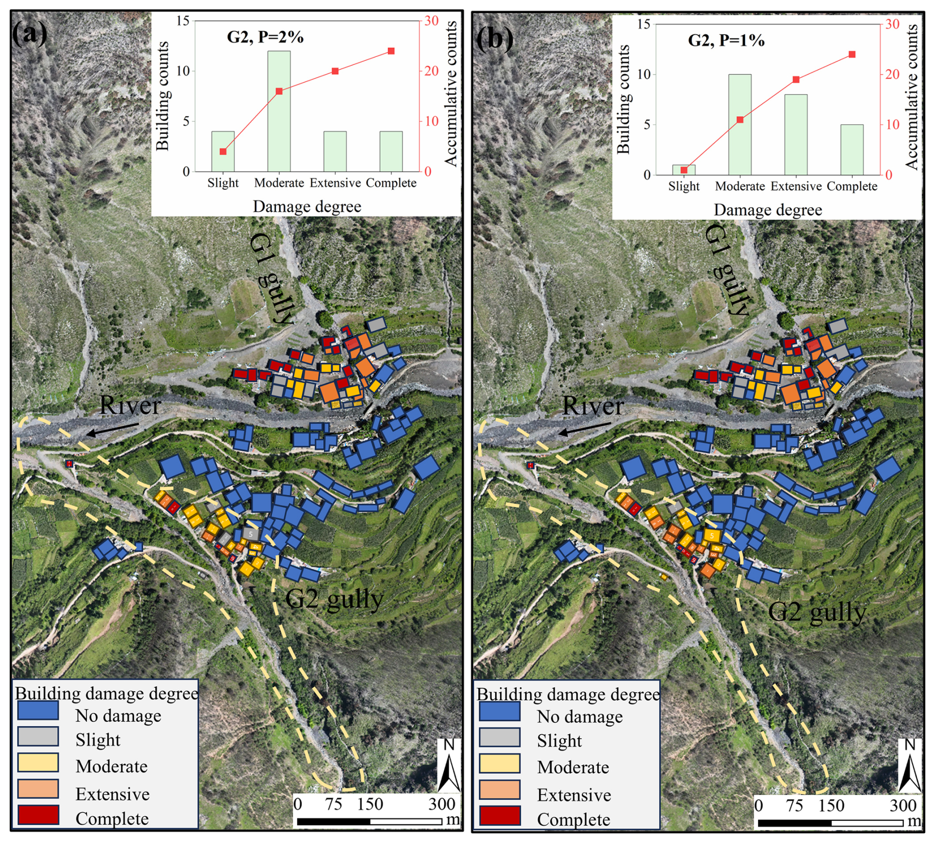
Figure 11 Predicted building counts with degree of damage and the spatial distribution in the G2 gully under different recurrence periods: (a) P = 2 %; (b) P = 1 %.

4 Discussion

4.1 Comparison of building vulnerability models

Firstly, we compared different debris flow intensity indicators. As mentioned earlier, we selected six indicators of the debris flow intensity to construct a building vulnerability model, but the vulnerability values also varied among the different indicators. Figure 12 shows the statistics of the total number of buildings and the vulnerability value under six debris flow intensities and four damage degrees in the G1 and G2 gullies of Kule village. The line width indicates the number of damaged buildings and their vulnerability value, with a thicker line indicating a higher value. The buildings in Kule village mainly exhibited moderate and complete damage.

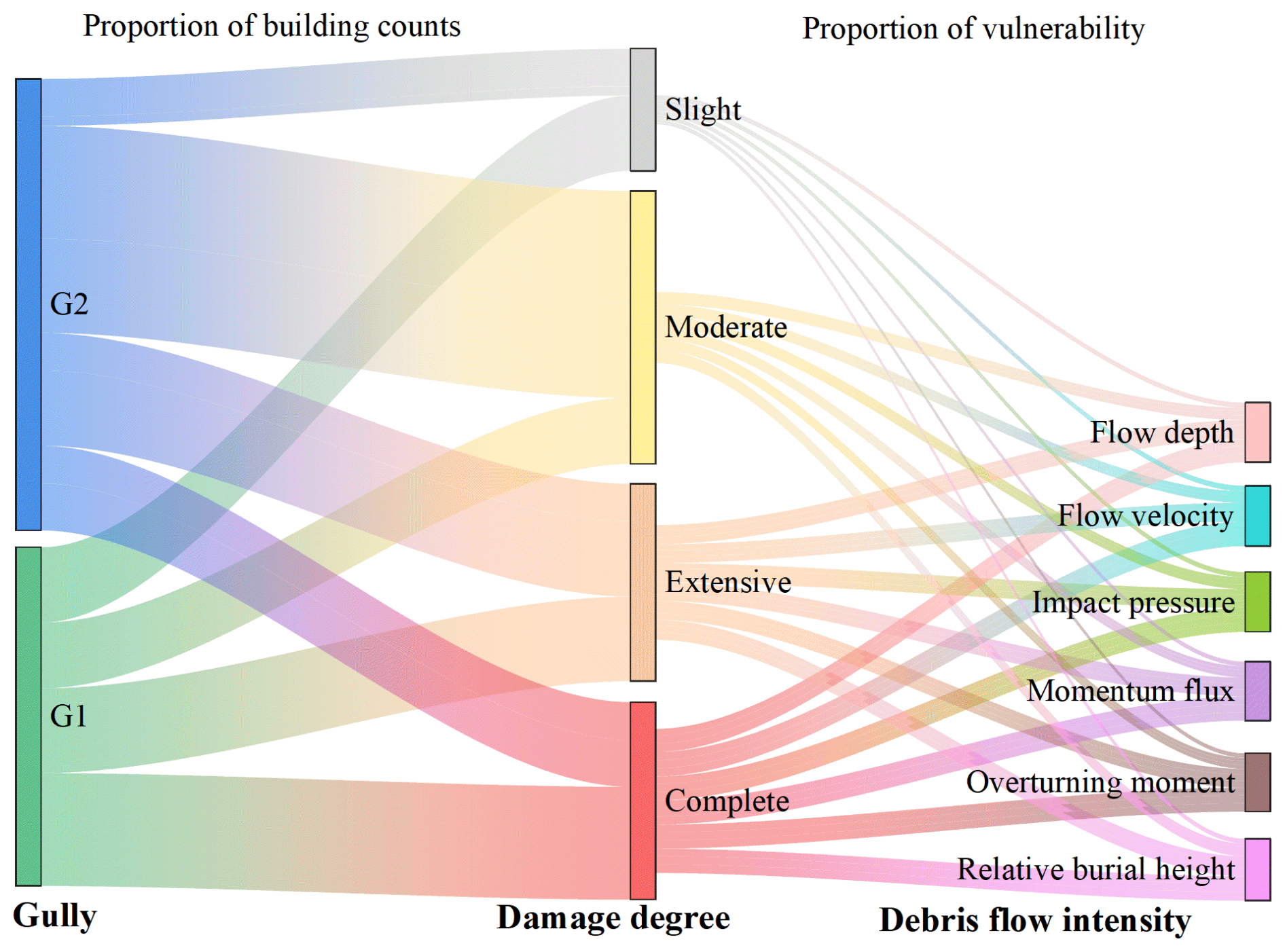
Figure 12 Statistics on the number of buildings and vulnerability under different debris flow intensities and damage degrees in the G1 and G2 gullies of Kule village.

The differences and sensitivities of the six curves in evaluating the vulnerability of damaged buildings are compared (Fig. 13). In terms of the properties of the normalized LNCDF curves, the larger the mean (μ) value is, the more the curve shifts to the right, indicating an increased probability of I^* attaining a larger value. The higher the standard deviation (σ) is, the flatter the curve and the more dispersed the probability distribution. Conversely, the lower σ, the steeper the curve is, indicating a narrower range of I^* values and a more concentrated probability distribution. As shown in Fig. 13, the momentum flux and overturning moment curves are steeper, indicating higher sensitivity of these indicators accompanied by a rapid increase in the probability of failure and more effective determination of the boundaries of the different damage categories (Barnhart et al., 2024). Additionally, the flow depth and impact pressure curves are relatively gradual, with low sensitivity, but the stability and accuracy of determining the degree of damage are greater (Wang et al., 2024; Lee et al., 2024). Furthermore, the impact pressure provides a more intuitive physical interpretation, indicating the destructiveness of debris flows in relation to both the hydrostatic pressure and dynamic overpressure, which has facilitated its widespread adoption in disaster risk assessment (Quan Luna et al., 2011; Wang et al., 2024).

Figure 13 Comparison of vulnerability curves of the normalized debris flow intensity.

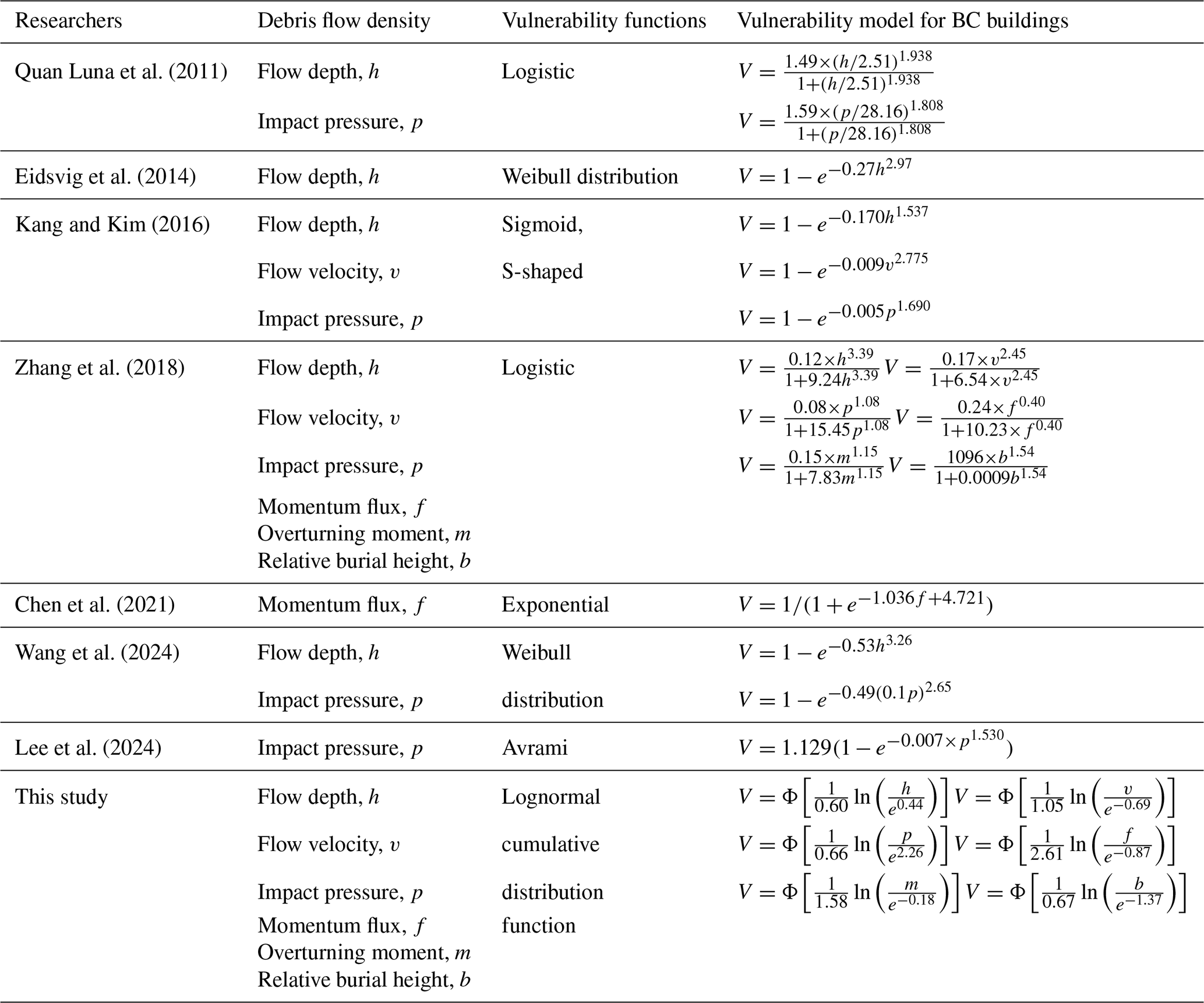
Secondly, we compared the proposed vulnerability model. Table 6 shows a comparison between the proposed vulnerability models for BC buildings and models established in previous studies (Quan Luna et al., 2011; Eidsvig et al., 2014; Kang and Kim, 2016; Zhang et al., 2018; Chen et al., 2021; Wang et al., 2024; Lee et al., 2024). Figure 14 shows a comparison of the proposed vulnerability curves for different debris flow intensities. For flow depth (Fig. 14a), our curve aligns closely with Quan Luna et al. (2011) and Zhang et al. (2018), while falling between the curves of Wang et al. (2024) and Kang and Kim (2016). The complete damage threshold (V = 0.8) occurs at 2.5 m in this study, compared to 1.3 m in Wang et al. (2024). For flow velocity (Fig. 14b), our curve exhibits a steeper slope than those of Zhang et al. (2018) and Kang and Kim (2016). The impact pressure curve (Fig. 14c) shows an initially steep slope similar to Zhang et al. (2018), then flattens as it approaches complete damage, reaching 25 kPa at V = 0.8. This value is lower than the 30 kPa reported by Quan Luna et al. (2011), Kang and Kim (2016), and Lee et al. (2024). For momentum flux (Fig. 14d), our curve resembles that of Chen et al. (2021) but lies well below Zhang et al. (2018). Complete damage (V = 1.0) occurs at 90 m³ s⁻² in this study, compared to 131 m³ s⁻² in Zhang et al. (2018). The overturning moment curve (Fig. 14e) is steeper than that of Zhang et al. (2018), reaching V = 0.8 at 4.0 m³ s⁻¹ compared to 20.1 m³ s⁻¹. For relative burial height (Fig. 14f), our curve is considerably steeper than Zhang et al. (2018).

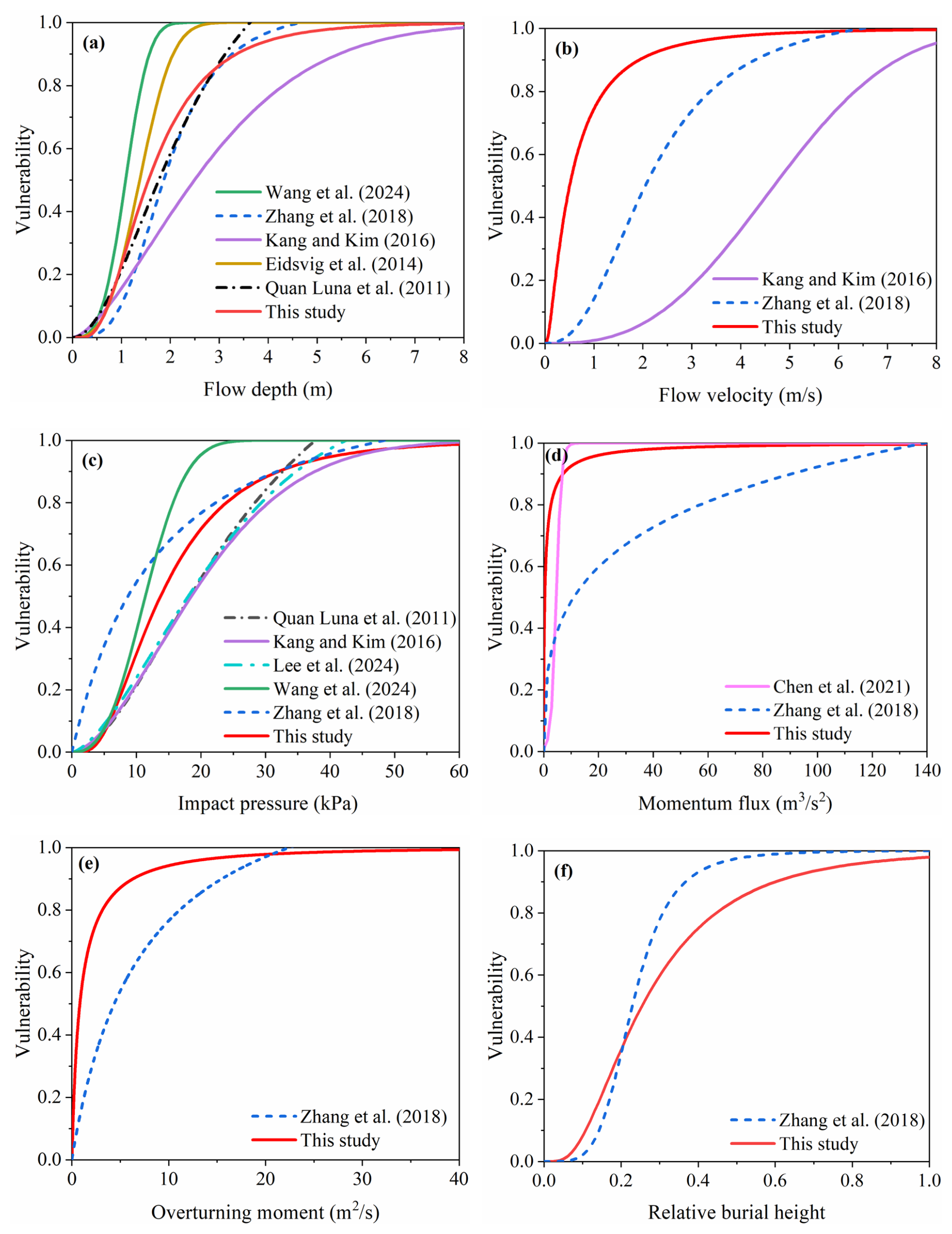
Figure 14 Comparison of the vulnerability curves with previous models for different debris flow intensities.

The observed differences between our vulnerability curves and those established in previous studies may be attributed to a combination of factors. At a general level, variations in regional building codes, construction practices, building geometry, and debris flow characteristics (e.g., volume, density, event scale) across study areas can influence vulnerability thresholds (Kang and Kim, 2016; Zhang et al., 2018). However, the distinct nature of postfire debris flows in this study likely plays a more important role. Wildfires alter watershed conditions in ways that increase the complexity and variability of debris flow processes. First, fire increases the proportion of loose, fine particles in surface soil (Ouyang et al., 2023), which are easily entrained and lead to higher solid concentrations and a greater tendency for deposition and building inundation. This may explain the higher complete damage thresholds observed for flow depth and relative burial height. Second, fire-damaged root systems and reduced slope infiltration capacity result in more pronounced sheet erosion and numerous small runoffs after rainfall, subjecting buildings to multi-directional and uneven impacts. Burned basins also exhibit lowered rainfall thresholds for debris flow initiation, leading to higher event frequency over extended periods (Fraser et al., 2022; Ouyang et al., 2023). These factors likely contribute to the steeper slopes of our flow velocity and overturning moment curves. Third, high temperatures from fire can weaken building envelopes, lowering their initial resistance to dynamic impact. This may explain the lower impact pressure (25 kPa) required to reach V = 0.8 and the lower momentum flux threshold (90 m³ s⁻²) for complete damage compared to non-postfire settings. Collectively, these postfire-specific mechanisms introduce greater variability into intensity-damage relationships and explain the deviations between our curves and those derived from non-postfire settings.

Table 6 Comparison of the vulnerability curves of brick-concrete buildings for different debris flow intensities between this study and previous studies.

Finally, the differences between the various vulnerability curves also depend on the vulnerability function models employed. Table 7 provides the existing vulnerability function models, including Logistic, Weibull, Exponential, LNCDF and Avrami functions (Quan Luna et al., 2011; Eidsvig et al., 2014; Kang and Kim, 2016; Zhang et al., 2018; Chen et al., 2021; Luo et al., 2023; Wang et al., 2024; Lee et al., 2024). We analysed the performance of the function models using data from this study and previous research (Fig. 15). The performance values of different function models were compared using the flow depth and impact pressure as examples (Fig. 15). The S-shaped function models (Logical, Weibull, Avrami and LNCDF models) clearly performed better than the exponential function model did, whose vulnerability curve did not pass through the origin (Fig. 15a, b) and may be heavily affected by outliers. In addition, the coefficients of determination of all the function models did not significantly differ, with R² values exceeding 0.88 (Table 7). This finding indicates that the coefficient of determination only focuses on the degree of fit of the regression equation (Lee et al., 2024), but it is not necessarily better for models with relatively large R² values, such as exponential functions (R² = 0.98) with relatively large errors. The coefficient of determination is affected by the complexity of the model, and overfitting may occur, which may lead to the model performing well for training data but exhibiting a poor prediction ability with new data. Therefore, the relative error and prediction accuracy of function models should be accounted for (Wang et al., 2018).

Table 7 Performance comparison between various data-driven building vulnerability function models.

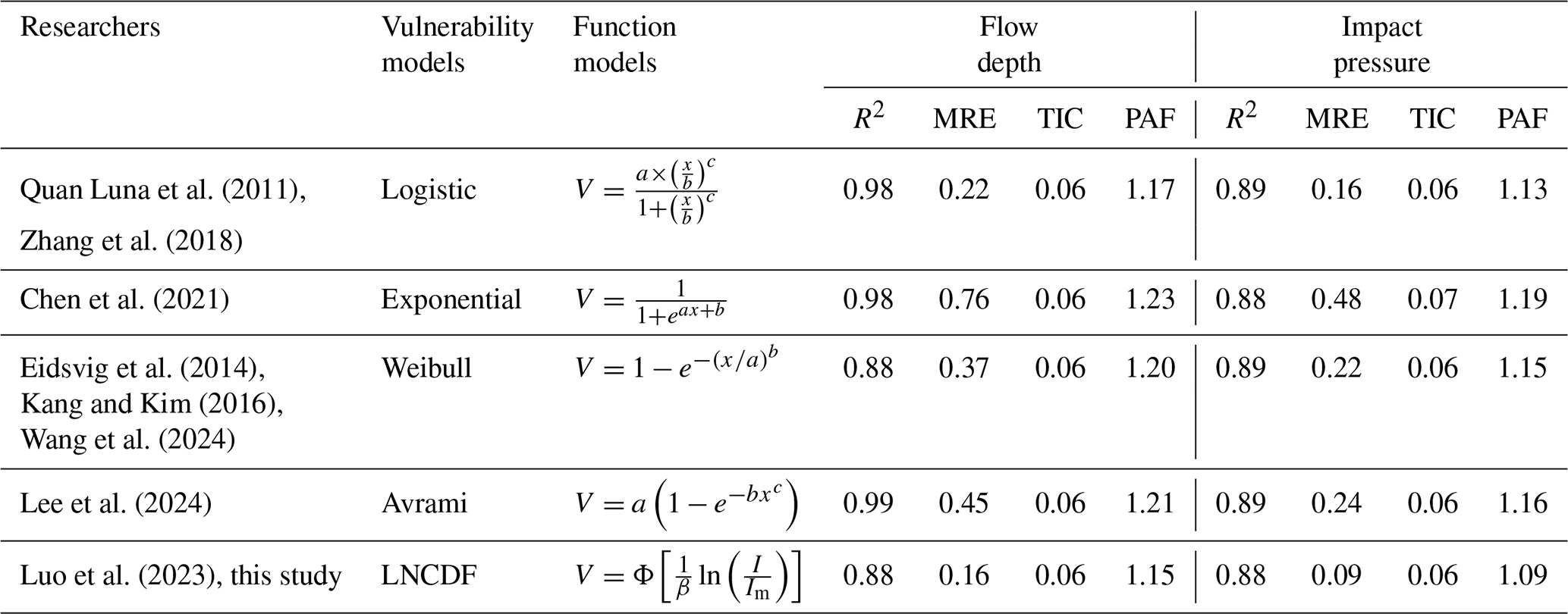
Note: the parameters a, b, and c can be obtained directly by curve fitting.

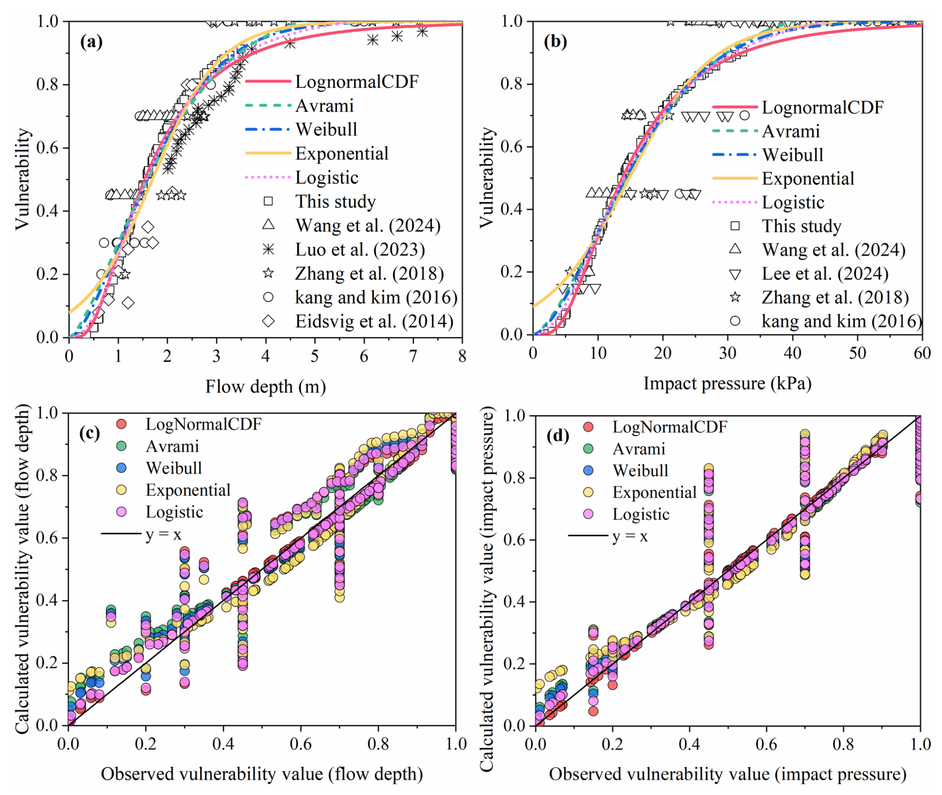
Figure 15 Performance comparison between different vulnerability function models: (a) flow depth vulnerability models; (b) impact pressure vulnerability models; (c) observation and calculation values of flow depth; (d) observation and calculation values of impact pressure.

In the comparison of the calculated and observed values, both the exponential and Avrami functions clearly exhibited significant errors (Fig. 15c, d). Specifically, the MRE values for the flow depth were 0.76 and 0.45, respectively, whereas the MRE values for the impact pressure were 0.48 and 0.24, respectively (Table 7). However, the LNCDF model demonstrated the highest statistical significance in terms of the relative error and accuracy, with MRE = 0.16 and PAF = 1.15 for the flow depth and MRE = 0.09 and PAF = 1.09 for the impact pressure. In multiple regression models, the coefficient of determination emphasizes the interpretability and fitting performance, whereas the error prioritizes the prediction accuracy of the model. Overall, these two metrics provide complementary insights for evaluating the overall performance of the model. Overall, the performance of the various function models exhibited the following order: LNCDF > logistic > Weibull > Avrami > exponential models. LNCDF-based models are insensitive to single data points because of the statistical parameter curve fitting process for developing these models. It has been demonstrated that the LNCDF model can efficiently increase the prediction performance, leading to a substantial reduction in output uncertainty, and this model is recommended for future applications (Kean et al., 2019; Luo et al., 2023).

4.2 Disaster reduction and emergency response suggestions

Both sides of Kule village are at risk of being impacted by the G1 and G2 gullies (Fig. 16). Owing to the impact of wildfires, there is a large amount of loose material in these gullies, which can trigger postfire debris flows again under low rainfall thresholds. Through the above field investigations and simulation predictions, debris flows can seriously damage buildings downstream of the alluvial fan and even block the Kule River, posing a severe threat to the lives of more than 300 people in the village. The most dangerous situation occurs when debris flows occur in the two gullies simultaneously (Fig. 16a). An immediate emergency response is crucial, and the escape route should be oriented along the vertical direction of the debris flow channel for reaching a safe location in high terrain (Fig. 16b). Left-bank residents should evacuate from both sides, thereby avoiding crossing the river. In contrast, right-bank residents should evacuate swiftly from the high-terrain area on their side. The safest suggestion is for residents to leave the village under feasible conditions. In the long term, reforestation can stabilize soil and reduce sediment into channels (Yang et al., 2022; Vahedifard et al., 2024). Thus, restoring vegetation in burned areas is essential for effectively suppressing postfire debris flows and promoting local ecological recovery (Yang et al., 2024).

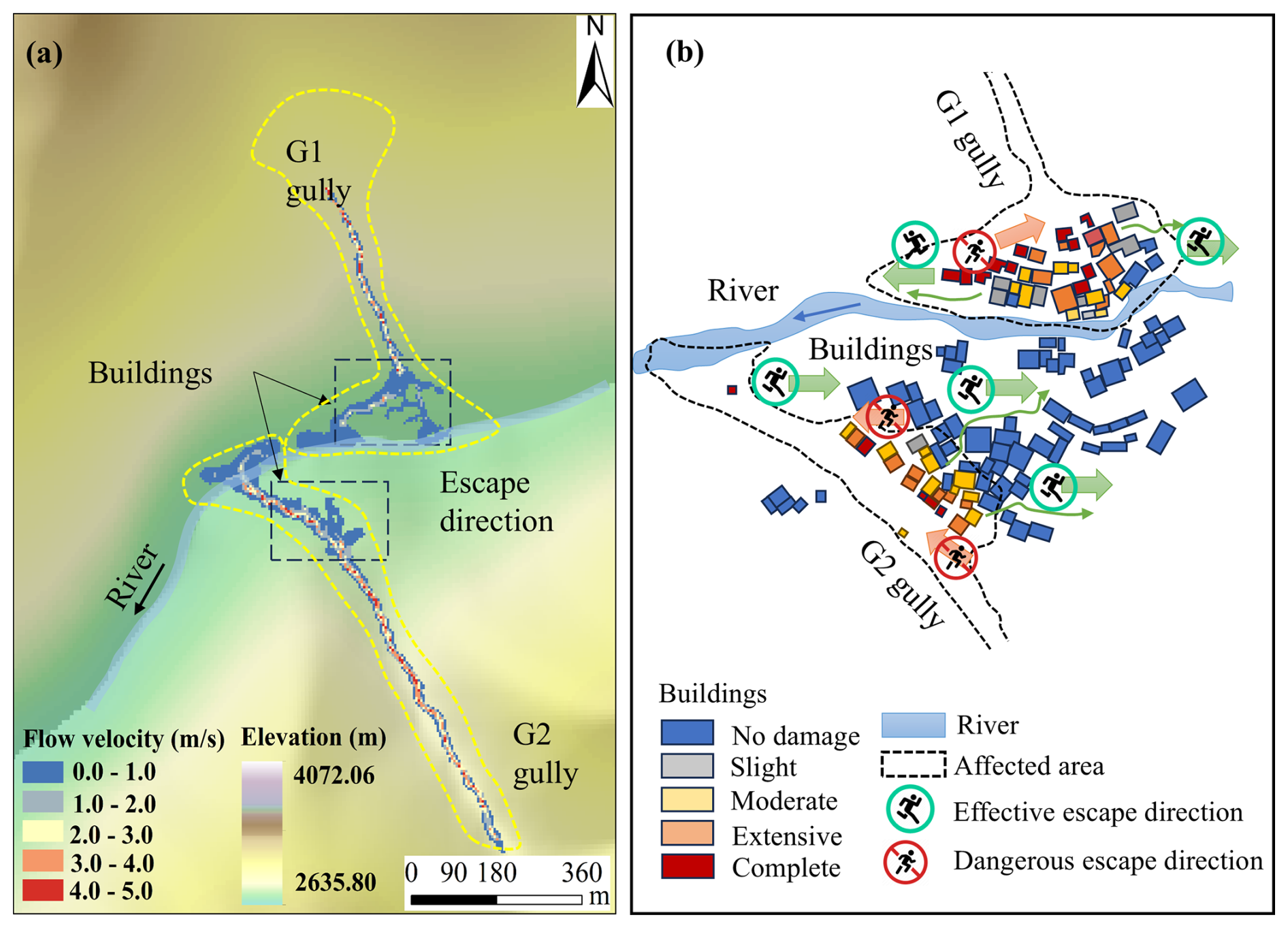
Figure 16 Disaster prediction and emergency response suggestions: (a) simulation of debris flows occurring simultaneously in the G1 and G2 gullies; (b) emergency response and risk avoidance suggestions for the residents of Kule village.

4.3 Limitations and future work

Our results provide insights into assessing the vulnerability of buildings to debris flows triggered by wildfires in Yajiang County. A combination of numerical simulation and function model methods provided a distinct advantage in the development of vulnerability curves. The spatial distributions of the flow depth and flow velocity can be visualized, and detailed physical information can be obtained in a specific area (Zhang et al., 2018). Additionally, this study highlights the importance of acknowledging and addressing the inherent uncertainty associated with various debris flow intensity indicators and function models applied in vulnerability assessments via a comparison of existing intensity indicators and evaluating the performance of various function models. Notably, while the methodological framework combining field investigation, numerical simulation, and vulnerability analysis is transferable to non-fire areas, the specific vulnerability curve parameter values require recalibration when applied elsewhere.

However, several limitations should be acknowledged. First, during the numerical modelling phase, terrain changes and sediment volume variations caused by debris flow entrainment were neglected (Wang et al., 2024), and validation focused on depositional area and runout volume, neglecting flow velocity along the path (Chen et al., 2021). Additionally, due to limited understanding of postfire debris flow triggering and runoff mechanisms (Rengers et al., 2016; Ouyang et al., 2023) and the introduction of burned wood into channels (Rengers et al., 2023), only volume and peak flow were considered as recurrence period indicators (Cui et al., 2018; Gorr et al., 2024), while other geological variables (e.g., particle size distribution, viscosity, water content) were not incorporated (Chen et al., 2021). Second, differences in the vulnerability curves of different indicators could cause uncertainty in vulnerability assessments (Luo et al., 2023), where the percentage of buildings categorized may be inconsistent. The slopes of the LNCDF-based curves increase slowly during the latter half, and intensity calculations based on maximum values may lead to overestimation of ultimate failure strength compared to actual values (Chen et al., 2021). Owing to the limited number of data points, to increase the reliability of the vulnerability curves (Lee et al., 2024; Ettinger et al., 2016), more data on postfire debris flow events and validations are needed in the future. Additionally, transferring the G1-calibrated parameters to G2, an approach based on field observations of comparable conditions between the adjacent catchments, introduces uncertainty as G2 is potentially hazardous but has not yet experienced a debris flow. The G2 simulation results show consistent orders of magnitude with similar regional events data (He et al., 2024). Direct validation of G2 predictions warrants attention in future work. Finally, this study focused on BC buildings, not accounting for other structural types (e.g., reinforced concrete frame buildings), mechanical failure criteria for unreinforced masonry walls (Si et al., 2022), or building-specific factors such as shape, orientation, number of floors, masking effects of building complexes and construction codes (Lee et al., 2024; Wang et al., 2024). These limitations emphasize the need for further research to enhance the comprehensive management of hazard risks in mountainous rural areas.

Future research should focus on ensuring continuous, standardized post-event data collection processes, which will enhance the practical applicability of the developed vulnerability curves. Ultimately, this framework represents an important step towards developing physical vulnerability models, thereby providing comprehensive insights into the potential effects of future postfire debris flow events on buildings in similar regions and offering valuable guidance for formulating disaster management and mitigation strategies.

5 Conclusions

This study assessed the vulnerability of buildings to postfire debris flows in Kule village, Yajiang County. A physical vulnerability model for BC buildings was established to support effective disaster management and emergency evacuation strategies for the region. The conclusions are as follows:

• 1.

  Field investigations characterized postfire debris flow features in the G1 and G2 gullies and documented damage to 36 BC buildings in Kule village. The volume and peak discharge of postfire debris flows were calculated, and the damage degree of buildings was categorized using a range of vulnerability indices.

• 2.

  Dynamic runout processes were simulated using the FLO-2D numerical model, with the reconstructed results calibrated to ensure consistency with actual situations. The simulations captured the debris flow intensities, including the flow depth, flow velocity, impact pressure, momentum flux, overturning moment, and relative burial height.

• 3.

  Physical vulnerability curves for BC buildings damaged by postfire debris flows in the G1 gully were developed. The vulnerability model was subsequently applied to the G2 gully, to predict potential building damage scenarios and their spatial distributions, enabling emergency evacuation recommendations for Kule village in the event of simultaneous debris flows in both gullies.

• 4.

  Comparisons of different vulnerability curves, intensity indicators, and function models revealed that momentum flux was the most sensitive indicator for distinguishing damage categories, while impact pressure could provide more accurate vulnerability values. Among the function models, the LNCDF function model demonstrated the highest statistical performance (MRE = 0.09, PAF = 1.09).

• 5.

  The proposed vulnerability model exhibits certain limitations, emphasizing the importance of acknowledging and addressing the inherent uncertainty associated with various intensity indicators, function models, triggering and runoff mechanisms underlying postfire debris flows, and building structure and orientation in future research.

Appendix A

Table A1 Debris flow intensities and building damage degree in G1 gully.

Appendix B

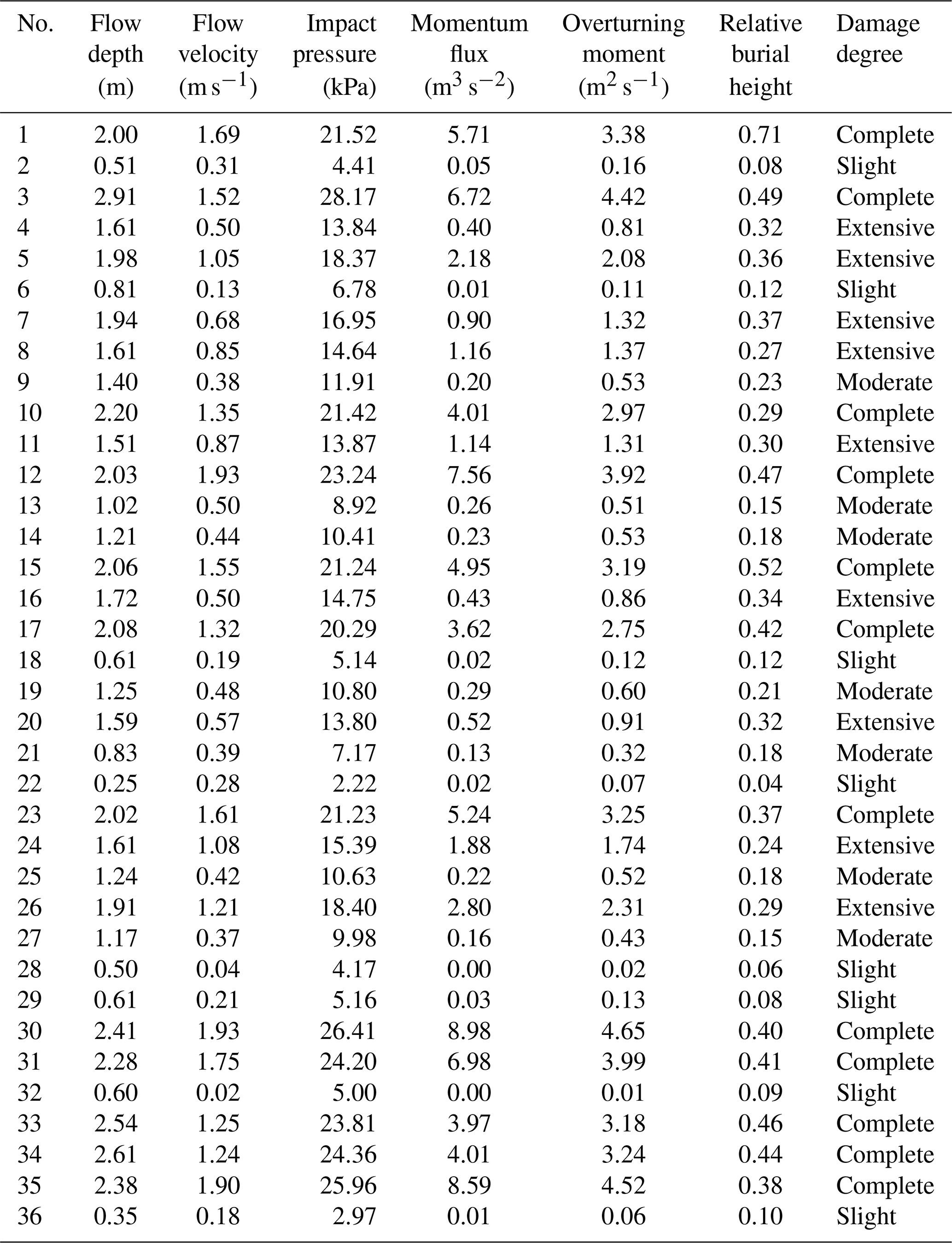
Table B1 Debris flow intensities and predicted building counts in G2 gully: (a) design frequency P = 1 %, (b) design frequency P = 2 %.