Evaluating the effects of preprocessing, method selection, and hyperparameter tuning on SAR-based flood mapping and water depth estimation

Flood mapping and water depth estimation from Synthetic Aperture Radar (SAR) imagery are crucial for calibrating and validating hydraulic models. This study uses SAR imagery to evaluate various preprocessing (especially speckle noise reduction), flood mapping, and water depth estimation methods. The impact of the choice of method at different steps and its hyperparameters is studied by considering an ensemble of preprocessed images, flood maps, and water depth fields.

The evaluation is conducted for two flood events on the Garonne River (France) in 2019 and 2021, using hydrodynamic simulations and in-situ observations as reference data. Results show that the speckle filtering method choice can significantly alter flood extent estimations with variations of several square kilometers. Additionally, the selection and tuning of flood mapping methods significantly affect performance. While supervised methods outperformed unsupervised ones, well-tuned unsupervised approaches (such as local thresholding or change detection) can achieve comparable results. The compounded uncertainty from preprocessing and flood mapping steps also introduces substantial variability in the water depth field estimates.

This study highlights the importance of considering the entire processing pipeline, encompassing preprocessing, flood mapping, and water depth estimation methods and their associated hyperparameters. Rather than relying on a single configuration, adopting an ensemble approach and accounting for methodological uncertainty should be privileged. For flood mapping, the method choice has the most influence. For water depth estimation, the most influential processing step was the flood map input resulting from the flood mapping step and the hyperparameters of the methods.

1 Introduction

Flood risk management largely benefits from accurate, timely, and spatially extensive observations of flood events. Satellite remote sensing allows the monitoring of large areas with increasing spatial and temporal resolution. Among the various types of satellite sensors, Synthetic Aperture Radar (SAR) sensors are particularly valuable for flood monitoring (Oberstadler et al., 1997; Bates, 2012). Unlike optical sensors, SAR sensors acquire images regardless of cloud coverage and daylight, making them suitable for detecting flood events with high spatial resolution (Tarpanelli and Benveniste, 2019). Flood mapping with SAR imagery exploits the interaction between the emitted signal and water surfaces, which typically results in dark spots in the images due to specular reflection where the smooth water surface mirrors the signal away from the sensor (Hostache et al., 2009; Mason et al., 2009; Martinis, 2010).

Numerous methods have been developed to extract flood maps from SAR imagery, including global and local thresholding methods (Chini et al., 2017; Mason et al., 2012), active contour models (Horritt, 1999), change detection methods (Giustarini et al., 2012; Bovolo and Bruzzone, 2007) or supervised classification approaches (Bentivoglio et al., 2022; Mateo-Garcia et al., 2021; Bonafilia et al., 2020). These flood maps provide essential data for model calibration and validation (Di Baldassarre et al., 2009; Montanari et al., 2009), and data assimilation in hydraulic forecasting systems (Hostache et al., 2010; Lai et al., 2014; Giustarini et al., 2011; Dasgupta et al., 2021).

Beyond generating flood maps, estimating water depth from SAR data is also valuable for hydraulic model calibration and validation (Hostache et al., 2009; Schumann et al., 2007; Betterle and Salamon, 2024). These estimations usually involve combining flood maps and ancillary datasets, such as Digital Elevation Models (DEMs) (Hostache et al., 2009; Schumann et al., 2007; Betterle and Salamon, 2024) or outputs from hydrodynamic simulations (Brown et al., 2016).

However, extracting hydraulic information such as flood maps and water depth fields from SAR images is subject to various sources of uncertainty. These include measurement noise (e.g., speckle), terrain-induced distortions, vegetation, and infrastructure influence. Furthermore, uncertainty arises from methodological choices in the processing workflow, such as noise filtering strategy, flood mapping methods, and hyperparameter settings. In this work, we refer to hyperparameters as user-defined parameters (e.g., window size for speckle filtering, threshold level for flood classification) that govern the behavior of an algorithm, as opposed to model parameters that can be measured or estimated based on physical considerations or measurements. Previous studies attempted to quantify these uncertainties. For example, Schumann et al. (2008) propagated geolocation uncertainties to derive ensembles of flood maps and associated water depth. Similarly, Martinis et al. (2015b) compared various operational flood mapping strategies to study their relevance in operational contexts. Landuyt et al. (2018) compared flood mapping methods with hyperparameter tuning across multiple flood events in Ireland and the UK (comparison to Copernicus Emergency Mapping Service flood maps), highlighting that method performance was highly variable depending on the study case and the fixed hyperparameters. Tupas et al. (2023), Chini et al. (2017) and Ghosh et al. (2024) drew the same conclusions when evaluating the role of hyperparameters in change detection, thresholding, and machine-learning based methods on the flood mapping outputs, respectively. However, flood studies rarely analyze the influence of preprocessing or hyperparameter tuning across the complete workflow, including flood mapping and water depth estimation. For instance, Landuyt et al. (2018) assume a unique preprocessing strategy for the satellite images without evaluating its role in the subsequent analysis.

In this study, we propose a comprehensive workflow for SAR-based flood analysis, evaluating the sensitivity of flood mapping and water depth estimation to different combinations of preprocessing, flood mapping, and water depth estimation methods. The objective is to quantify the uncertainty introduced at each stage of the SAR image processing and identify robust configurations for operational use. The preprocessing (speckle filtering), flood mapping, and water depth estimation methods were all evaluated for varying hyperparameter settings. This evaluation was carried out in an operational context with two flood events on the Garonne River in France in 2019 and 2021, with two Sentinel-1 SAR observations available for both flood events. All code and data are publicly available to facilitate reproducibility and further experimentation by the hydraulic modeling community at https://doi.org/10.5281/zenodo.20209044 (Travert et al., 2026).

This article is structured as follows. Section 2 describes the methodology and study area, including the satellite data and validation datasets. Section 3 describes and applies the SAR image preprocessing steps, explicitly focusing on speckle filtering strategies. Section 4 reviews and evaluates flood mapping approaches. Section 5 presents the estimation of water depths from SAR-derived flood maps using DEMs. Section 6 discusses limitations of this study and their operational use for model calibration. Finally, Sect. 7 provides conclusions and implications for operational flood monitoring.

2 Methodology

The general workflow for processing SAR satellite images for flood applications is illustrated in Fig. 1.

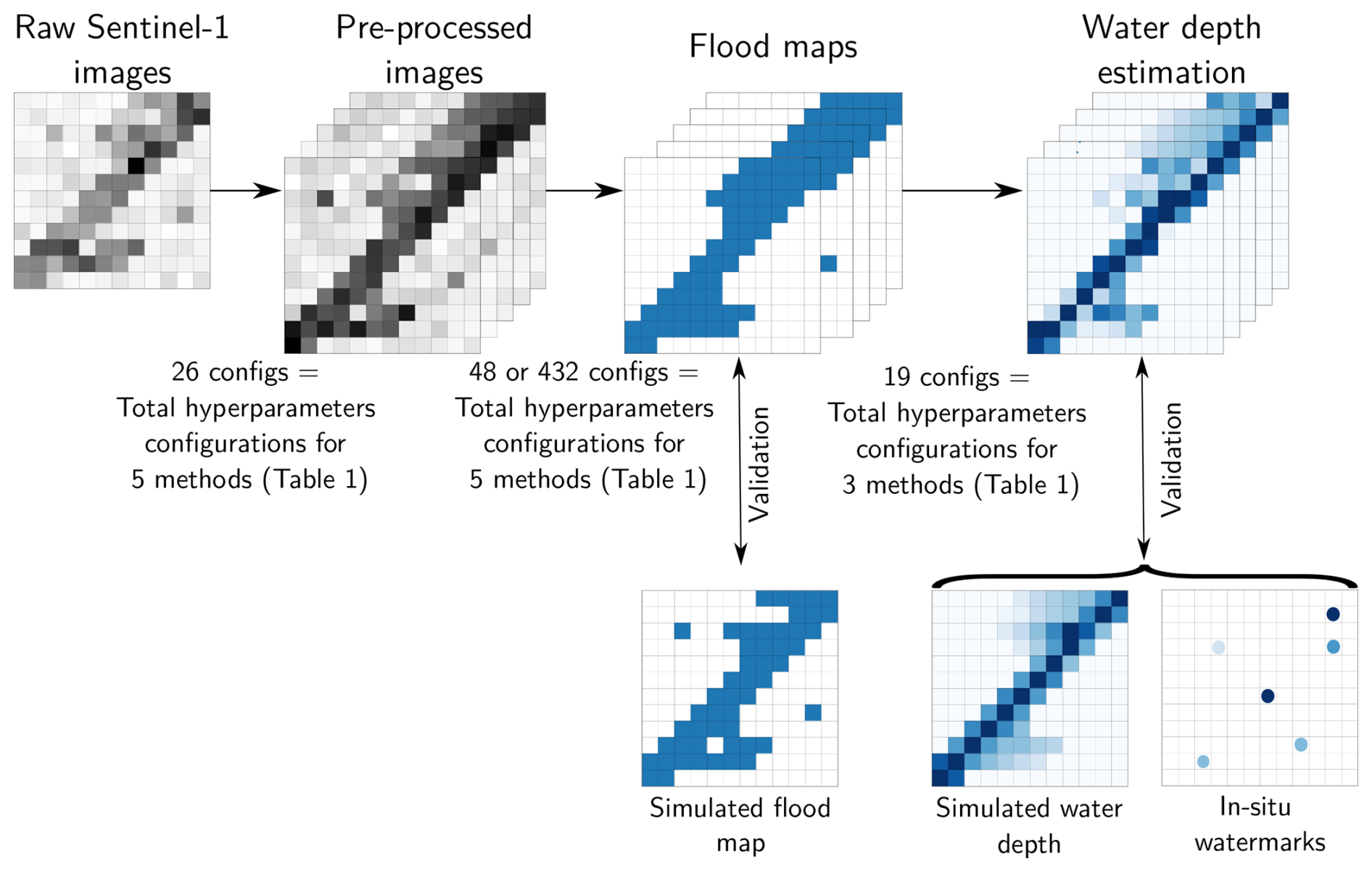
Figure 1 Workflow for processing Sentinel-1 (SAR) images to derive flood maps and water depth fields. Raw images are preprocessed using 26 hyperparameter configurations, then each image is turned into 48 flood maps (or 432 if using morphological operations). Each flood map is transformed into water depth fields using 19 configurations. The configurations are described in Table 1.

The workflow consists of the following steps:

1. SAR image preprocessing: Raw SAR images are first preprocessed to improve flood signal extraction. Five filtering methods were tested, including the Median filter, Lee filter (Lee, 1980), Lee Sigma filter (Lee et al., 2008), Frost filter (Frost et al., 1982), and the SAR2SAR deep-learning-based approach (Dalsasso et al., 2021). Each speckle filtering method was applied with a specific set of hyperparameters, resulting in 26 unique configurations: one configuration without any preprocessing (no hyperparameters), three configurations each for the Median and Lee filters, nine configurations each for the Frost and Lee Sigma filters, and one configuration for SAR2SAR.

2. Flood mapping: Each preprocessed image is used as input for flood mapping. Five methods were tested: global thresholding, local thresholding, active contour models, change detection, and supervised classification. These methods are also parameterized, resulting in an ensemble of flood maps for each preprocessed input. Post-processing morphological operations are optionally applied to remove isolated water pixels or small nonphysical holes caused by SAR speckle, geometric distortions, or flood map processing. In total, for each input preprocessed image, 48 flood mapping configurations are tested: one configuration each for the supervised classification models (no hyperparameters), two for global thresholding, two for change detection, six for active contour, and 36 for local thresholding. When using morphological post-processing, nine configurations were evaluated. With morphological operations, 432 flood mapping outputs (48×9) were generated per preprocessed image.

3. Water depth estimation: Each flood map generated in the previous step, together with a Digital Elevation Model (DEM) including the bathymetry for the river channel, is used to estimate water depth fields using three methods: Fw-DET (Cohen et al., 2019), FLEXTH (Betterle and Salamon, 2024), and a cross-sectional hydraulic approach. For each input flood map, 19 water depth estimation configurations are tested: one configuration for the cross-section approach (no hyperparameters), nine for Fw-DET, and nine for FLEXTH.

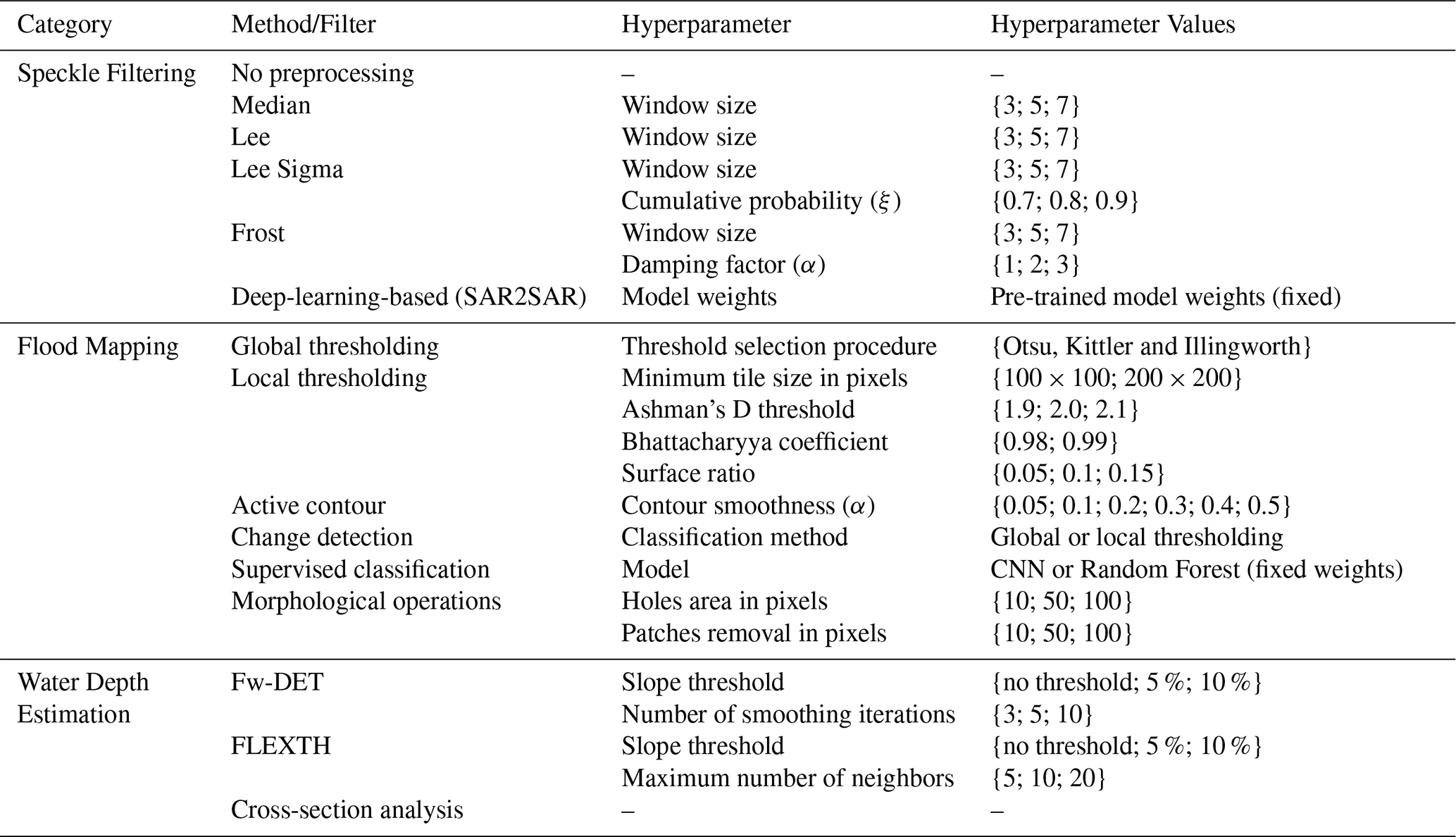
The preprocessing, flood mapping, and water depth estimation methods are described in more details in Sects. 3, 4 and 5 respectively. All the methods and their respective hyperparameters are summarized in Table 1. Although validation datasets, such as hydrodynamic simulations, were used to support a better understanding of the methodology, the main focus of the study was to explore the variability in outputs resulting from these choices, rather than to perform a strict validation. The range of the hyperparameters is based on classical values used in the literature to avoid non-physical hyperparameter values.

Table 1 Overview of speckle filtering, flood mapping, and water depth estimation methods used in this study along with their associated hyperparameter sampling.

2.1 Study area and materials

The study area was the Garonne River between Tonneins and La Réole, in southwest of France (see Fig. 2). In this section of the river, the river width is around 250 m and the floodplain is 1–4 km wide, mainly comprises rural areas used for agricultural purposes. Since the end of the nineteenth century, the area has been equipped with dikes to protect urban areas and infrastructures. The floodplain, aside from the presence of dikes, displays minimal topographic variation.

2.1.1 Satellite observations

The study area was observed during two flood events in December 2019 and early February 2021 by the Sentinel-1 C-band Synthetic Aperture Radar (SAR) instrument at 5.405 GHz. The extent of the study area and the satellite image acquisitions are visualized in Fig. 2. Sentinel-1 “Ground Range Detected” products were downloaded from ASF Data Search Vertex (https://search.asf.alaska.edu/, last access: 26 May 2026) in VH polarization. The role of polarization is beyond the scope of this study. Most flood mapping methods rely on the analysis of a single polarization image. Accordingly, the VH polarization was used since, in the literature, VH polarization better distinguishes flooded from dry areas than VV polarization (Henry et al., 2006). Two additional Sentinel-1 images, acquired under non-flooded conditions, were used as references for one of the flood mapping methods. For the 2019 event, the reference image was acquired on 10 December 2019. For the 2021 event, the reference observation was acquired on 28 January 2021. Each image consists of an N_x×N_y grid of pixels, with a spatial resolution of 10×10 m. The images are projected onto a common grid that covers the entire study area. Here, the image's dimensions are N_x=2644 and N_y=2312. All times reported below are given in Coordinated Universal Time (UTC).

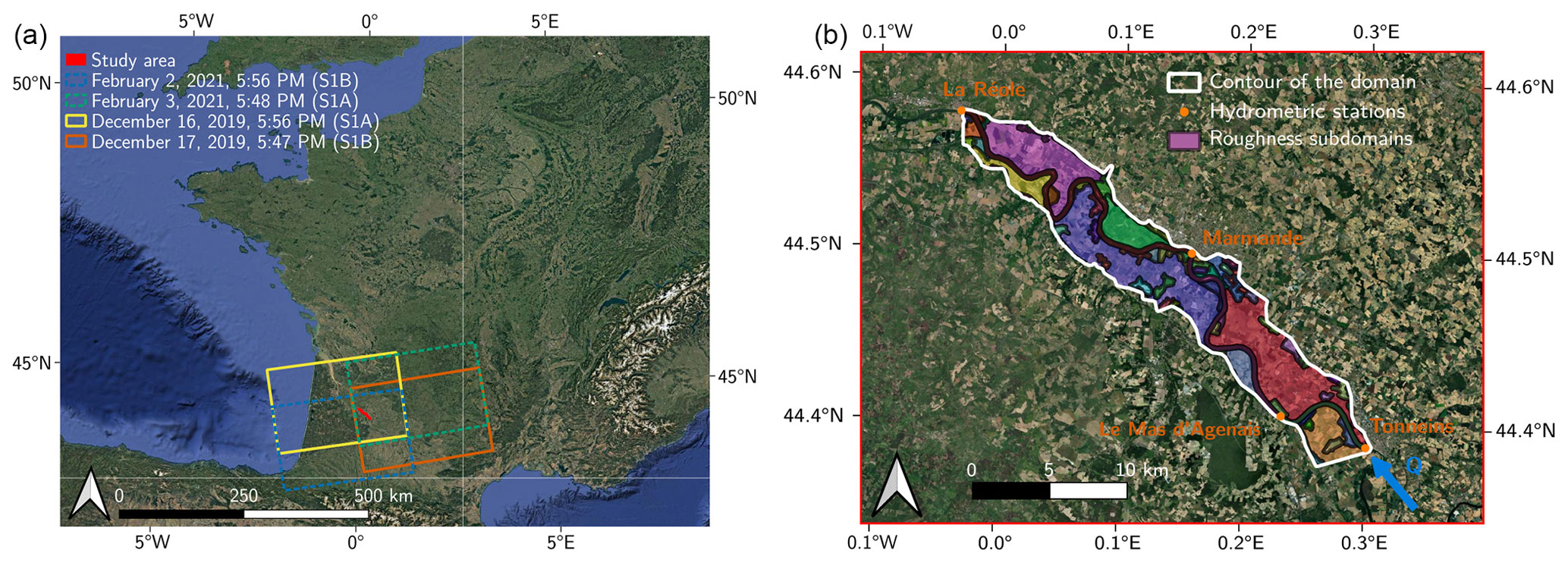
Figure 2 Visualization of the study area on the Garonne River in France with (a) the extent of the Sentinel-1 A (S1A) and Sentinel-1 B (S1B) acquisitions during 2019 and 2021 flood events and (b) a zoom-in on the study area with in-situ stage gauging stations and roughness subdomains.

2.1.2 Validation data

For comparing the observed flood maps and water depth fields derived from satellite images, observed water marks and stage gauging stations are available. These observations were also compared to simulated flood maps and water depth fields. The simulations are not the ground truth, but serve as a reference for comparison. The main goal of the study is to compare the variability of the outputs due to preprocessing, method choices, and hyperparameters, so the validation dataset is not the most important. We describe these datasets below.

Watermarks are visible traces left on buildings, trees, or other infrastructures during a flood event at the peak water level. For both the 2019 and 2021 flood events, watermarks were collected and made available on the French collaborative platform “Repères de Crues” (https://www.reperesdecrues.developpement-durable.gouv.fr/, last access: 26 May 2026). For the 2019 and 2021 flood events, 121 and 178 are available, respectively. For both events, satellite images were acquired near the flood peak (17 December 2019 and 3 February 2021), so the watermarks should coincide with the water depths extracted from the satellite images.

Three stage-gauging stations are available in the study area (Tonneins, Marmande, and La Réole). Discharge and water level data at these locations during the flood events are available on Vigicrues (https://www.vigicrues.gouv.fr/, last access: 26 May 2026, a flood-monitoring service that collects watermarks during floods in France). The measured discharges at the three stations for both flood events are shown in Fig. 3.

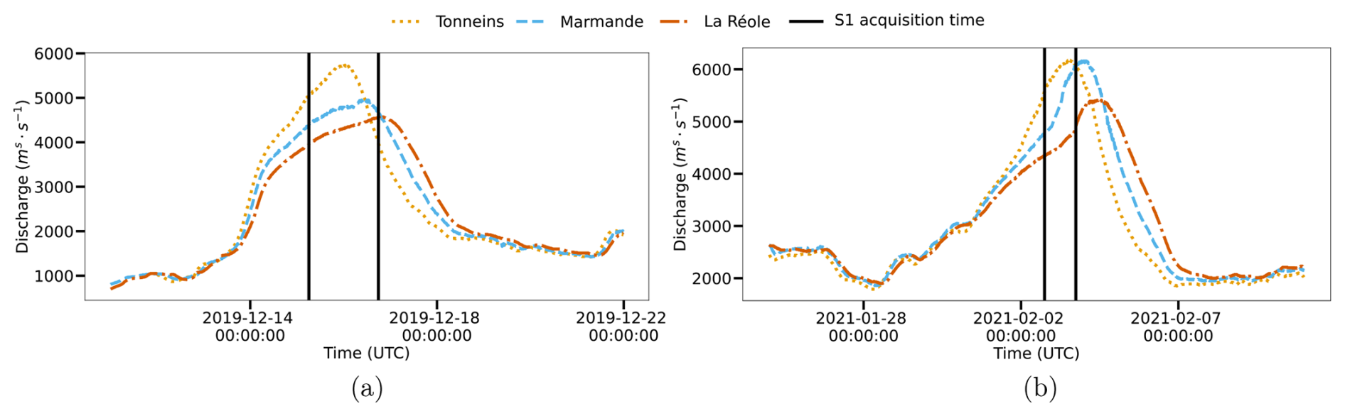
Figure 3 Measured discharge at gauging stations (Tonneins, Marmande, and La Réole) during the (a) December 2019 and (b) February 2021 flood event.

For flood simulations, a numerical solution of the Shallow Water Equations (SWEs) was used and solved with TELEMAC-2D, part of the openTELEMAC open-source hydrodynamic modeling system (https://www.opentelemac.org/, last access: 26 May 2026) (Hervouet, 2007). The SWEs are expressed in Cartesian coordinates where gravity acts uniformly in the vertical direction as −ge_z:

$$\begin{array}{}\text{(1)}& {\displaystyle \frac{\partial h}{\partial t}}+{\displaystyle \frac{\partial \left(hu\right)}{\partial x}}+{\displaystyle \frac{\partial \left(hv\right)}{\partial y}}=\mathrm{0},\end{array}$$

$$\begin{array}{}\text{(2)}& \begin{array}{rl}& {\displaystyle \frac{\partial \left(hu\right)}{\partial t}}+{\displaystyle \frac{\partial \left(h{u}^{\mathrm{2}}\right)}{\partial x}}+{\displaystyle \frac{\partial \left(huv\right)}{\partial y}}=-gh{\displaystyle \frac{\partial \mathit{\eta }}{\partial x}}\\ & +\mathrm{\nabla }\cdot \left(h{\mathit{\nu }}_e\mathrm{\nabla }u\right)-{\displaystyle \frac{\mathrm{1}}{\mathit{\rho }}}{\mathit{\tau }}_{\mathrm{b}x},\end{array}\end{array}$$

$$\begin{array}{}\text{(3)}& \begin{array}{rl}& {\displaystyle \frac{\partial \left(hv\right)}{\partial t}}+{\displaystyle \frac{\partial \left(h{v}^{\mathrm{2}}\right)}{\partial y}}+{\displaystyle \frac{\partial \left(huv\right)}{\partial x}}=-gh{\displaystyle \frac{\partial \mathit{\eta }}{\partial y}}\\ & +\mathrm{\nabla }\cdot \left(h{\mathit{\nu }}_e\mathrm{\nabla }v\right)-{\displaystyle \frac{\mathrm{1}}{\mathit{\rho }}}{\mathit{\tau }}_{\mathrm{b}y}.\end{array}\end{array}$$

The system unknowns are the water depth h≥0 and the depth-averaged velocity ue_x+ve_y both functions defined as functions of spatial coordinates x, y and time $t\in [\mathrm{0},T)$. The water surface is denoted by $\mathit{\eta }=h+z_{\mathrm{b}}$, where z_b(x,y) is the prescribed bottom elevation. A constant viscosity ν_e>0 is assumed, and the bed shear stress is expressed as τ_bxe_x+τ_bye_y depending on the variables h, u, and v. The bed shear stress is computed using Manning-Strickler formulation (Manning et al., 1890):

$$\begin{array}{}\text{(4)}& \left\{\begin{array}{l}{\mathit{\tau }}_{\mathrm{b}x}=\frac{\mathit{\rho }\cdot g\cdot u}{h^{\mathrm{1}/\mathrm{3}}\cdot K_{\mathrm{s}}^{\mathrm{2}}}\sqrt{u^{\mathrm{2}}+v^{\mathrm{2}}}\\ {\mathit{\tau }}_{\mathrm{b}y}={\displaystyle \frac{\mathit{\rho }\cdot g\cdot v}{h^{\mathrm{1}/\mathrm{3}}\cdot K_{\mathrm{s}}^{\mathrm{2}}}}\sqrt{u^{\mathrm{2}}+v^{\mathrm{2}}}\end{array}\right.,\end{array}$$

where K_s is the Strickler coefficient which varies spatially with x, and y (Morvan et al., 2008).

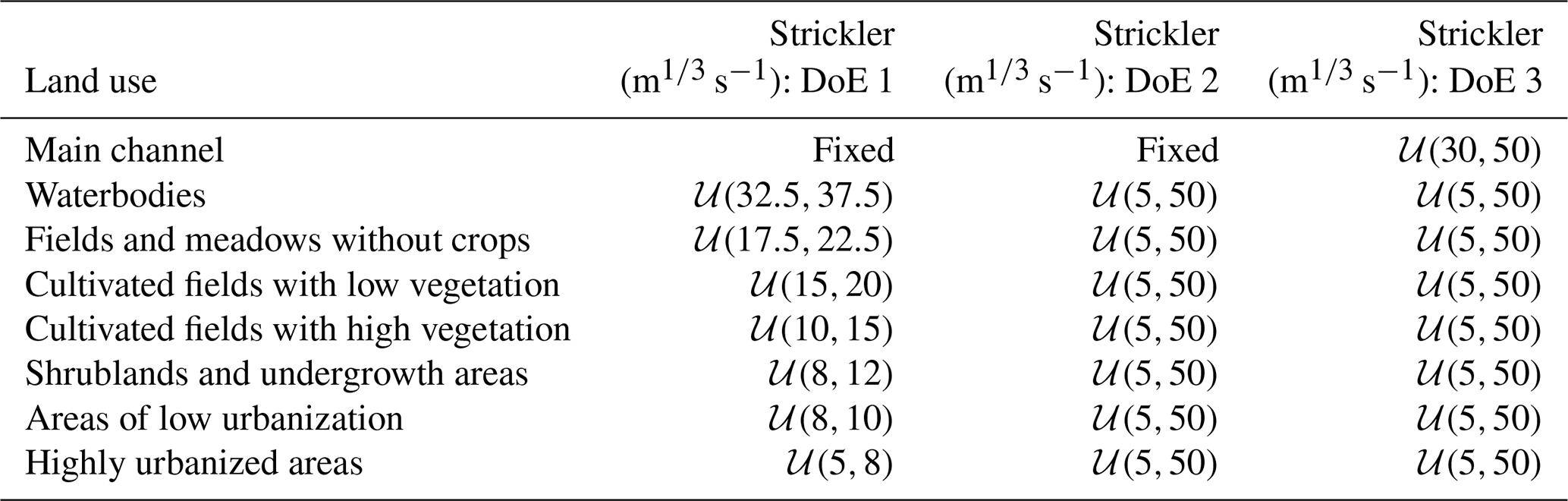
Upstream discharge was retrieved from the Tonneins stations for 11–21 December 2019 and 25 January–10 February 2021 and reported in Fig. 3. A rating curve was imposed at the downstream boundary. The simulations were initialized at t=0 with a base flow of 800 m³ s⁻¹ for the 2019 event, and 2300 m³ s⁻¹ for the 2021 event. One simulation was conducted for each flood event. The Strickler values were calibrated in previous studies for the river channel (Besnard and Goutal, 2011; El Garroussi et al., 2019; Nguyen et al., 2022), and are fixed in the floodplains based on the land use (Chow et al., 1988). The spatial distribution of Strickler values used in the simulation is reported in Fig. 2 and their values are described in Table 2 taking the median value of the Strickler value ranges of Design of Experiment 1. Bathymetry in the channel was reconstructed from 70 cross-sectional elevation profiles, and floodplain topography was obtained using data from IGN (the French National Institute of Geographic and Forest Information) combined with aerial imagery. The reader can refer to Besnard and Goutal (2011) and Travert et al. (2025) for more information on the construction and parameterization of the numerical model.

Table 2 Three tested Design of Experiments (DoE) for Strickler parameterization for numerical model evaluation. DoE 1 is the baseline with fixed channel values and narrow ranges in floodplains, DoE 2 accounts for wider ranges in floodplains, and DoE 3 also considers a varying Strickler across the three channel subdomains.

3 Satellite images preprocessing

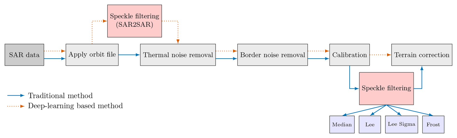
Synthetic Aperture Radar (SAR) images, such as those acquired by Sentinel-1, require several preprocessing steps to correct for sensor geometry, normalize radiometric responses, and suppress speckle noise. The processing chain adopted in the present study is presented in Fig. 4 and comprises sequential operations: application of orbit files, removal of thermal and border noise, radiometric calibration, speckle filtering, and terrain correction using the Range-Doppler method. In the processing workflow for terrain correction and georeferencing, a Digital Elevation Model of the study area at a 1 m resolution is used. Two alternative workflows were used depending on the speckle filtering strategy since the deep-learning-based speckle filtering (SAR2SAR method) was trained on images without preprocessing, while the other traditional filters were applied on calibrated images.

Figure 4 Preprocessing workflow for Sentinel-1 SAR images.

In SAR imagery, speckle noise, which arises from the coherent summation of scattered electromagnetic waves, is a well-known source of error. It resembles salt and pepper with dark and bright pixels (see Fig. 5). It alters the statistical properties of the image, preventing them from maintaining a consistent mean radiometric level in homogeneous areas (Bruniquel and Lopes, 1997). Speckle noise is modeled with a randomly fluctuating variable, such as (Goodman, 1976):

$$\begin{array}{}\text{(5)}& I_{i,j}=R_{i,j}\cdot S_{i,j},\end{array}$$

where $I\in {\mathbb{R}}^{N_x\times N_y}$ denotes the observed intensity (raw image), $R\in {\mathbb{R}}^{N_x\times N_y}$ the true radar backscatter, $S\in {\mathbb{R}}^{N_x\times N_y}$ the speckle component, and i,j the pixel locations. S_i,j and R_i,j are assumed to be statistically independent.

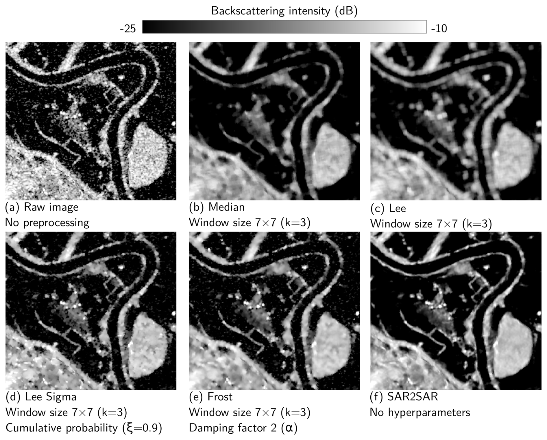
Figure 5 Backscatter intensity results from applying various speckle filters on a Sentinel-1 image in VH polarization.

3.1 Speckle filters methods

To mitigate the effects of noise, several speckle filters that aim to recover R the true radar backscatter while preserving image structures have been proposed in the literature. A review on speckle filtering methods is available in Deledalle et al. (2014) and Lee and Pottier (2017). In this study, we selected a representative set of widely used traditional filters such as Frost, Lee, Lee Sigma, and Median filter, due to their simplicity and strong track record in SAR image denoising. Additionally, we included a recent deep learning-based method to evaluate potential performance improvements from modern data-driven approaches. The characteristics of these filters are summarized in Table 1. In the following sections, each method is described in more detail.

The deep-learning based model (SAR2SAR model) was implemented via the deepdespeckling Python library available at https://pypi.org/project/deepdespeckling/ (last access: 26 May 2026) (Dalsasso et al., 2021). The other traditional filtering operations were conducted using the ESA SNAP toolbox. The complete preprocessing chain was automated using SNAP’s Graph Processing Tool (GPT) and Python scripting, facilitating large-scale processing of SAR image stacks.

3.1.1 Median filter

The Median filter replaces the center pixel with the median value of all pixels within a local scanning window, such that:

$$\begin{array}{}\text{(6)}& {\widehat{R}}_{i,j}=\mathrm{median}\left\{I_{m,n}|i-k\le m\le i+k,j-k\le n\le j+k\right\},\end{array}$$

with a window size of 2k+1 with k a non-negative integer. In this study, the window size is treated as a hyperparameter. The median filter is effective at removing isolated spot noise, but it tends to blur edges and erase thin linear features (Lee, 1983). To address this limitation, other approaches referred to as adaptive filters have been developed that incorporate local image statistics to better preserve structural details.

3.1.2 Lee filter

The Lee filter (Lee, 1980) accounts for the local statistics of the image within a moving window. From the multiplicative noise definition in Eq. (5), the mean and variance of R can be estimated, such as:

$$\begin{array}{}\text{(7)}& {\stackrel{\mathrm{‾}}{R}}_{i,j}={\stackrel{\mathrm{‾}}{I}}_{i,j},\mathbb{V}\mathrm{ar}\left(R_{i,j}\right)={\displaystyle \frac{\mathbb{V}\mathrm{ar}\left(I_{i,j}\right)-{\stackrel{\mathrm{‾}}{I}}_{i,j}^{\mathrm{2}}\mathbb{V}\mathrm{ar}\left(S_{i,j}\right)}{\mathbb{V}\mathrm{ar}\left(S_{i,j}\right)+{\stackrel{\mathrm{‾}}{S}}_{i,j}^{\mathrm{2}}}},\end{array}$$

where the quantities ${\stackrel{\mathrm{‾}}{I}}_{i,j}$ and 𝕍ar(I_i,j) are the local mean and variance of pixel intensities within a window of size 2k+1 centered at (i,j). In this study, the window size is treated as a hyperparameter. The Lee Filter assumes a linear estimator and using the local mean and variance within each scanning window, the estimator is written as:

$$\begin{array}{}\text{(8)}& {\widehat{R}}_{i,j}={\stackrel{\mathrm{‾}}{R}}_{i,j}+{\displaystyle \frac{\mathbb{V}\mathrm{ar}\left(R_{i,j}\right)}{\mathbb{V}\mathrm{ar}\left(I_{i,j}\right)}}(I_{i,j}-{\stackrel{\mathrm{‾}}{S}}_{i,j}{\stackrel{\mathrm{‾}}{R}}_{i,j}).\end{array}$$

The Lee filter aims to reduce speckle in homogeneous areas while preserving image details, such as edges and fine structures, in areas of high variance.

3.1.3 Lee Sigma filter

The Lee filter effectively reduces speckle noise but can cause blurry edges and loss of detail in heterogeneous areas. To address this issue, the Lee Sigma filter (Lee, 1983) was introduced. It calculates local statistics similarly to the Lee filter but using only the pixels whose intensities fall within a range to exclude outliers. The range is defined as $[{\stackrel{\mathrm{‾}}{R}}_{i,j}-\mathrm{2}\sqrt{\mathbb{V}\mathrm{ar}\left(S_{i,j}\right)}{\stackrel{\mathrm{‾}}{R}}_{i,j},{\stackrel{\mathrm{‾}}{R}}_{i,j}+\mathrm{2}\sqrt{\mathbb{V}\mathrm{ar}\left(S_{i,j}\right)}{\stackrel{\mathrm{‾}}{R}}_{i,j}]$. Because the a priori mean, ${\stackrel{\mathrm{‾}}{R}}_{i,j}$, is unknown, it is approximated by I_i,j, the value of the center pixel.

An improved version (Lee et al., 2008) relaxes the usual range and introduces a new interval (I₁,I₂) that meets two conditions:

• The interval captures a fixed cumulative probability ξ:

  $$\begin{array}{}\text{(9)}& \mathit{\xi }=\underset{I_{\mathrm{1}}}{\overset{I_{\mathrm{2}}}{\int }}p\left(I\right)\mathrm{d}I,\end{array}$$

  where p(I) is the empirical probability distribution of the pixel intensity computed on the scanning window.

• The mean within the interval must match the overall mean:

  $$\begin{array}{}\text{(10)}& \stackrel{\mathrm{‾}}{I}={\displaystyle \frac{\mathrm{1}}{\mathit{\xi }}}\underset{I_{\mathrm{1}}}{\overset{I_{\mathrm{2}}}{\int }}Ip\left(I\right)\mathrm{d}I.\end{array}$$

A value of ξ=0.8 or 0.9 is often used, but a lower value of ξ may be selected to preserve SAR image texture information and prevent potentially over-smoothing details (Lee et al., 2008). Two hyperparameters are used for the Lee Sigma filter, the window size and ξ.

3.1.4 Frost filter

Similarly to the Lee filter, the Frost filter (Frost et al., 1982) is based on the local statistics of the images and the multiplicative noise model. The Frost filter replaces a pixel value with a weighted sum of the values of its neighbors within a moving scanning window, such that:

$$\begin{array}{}\text{(11)}& {\widehat{R}}_{i,j}=\sum _{m=-k}^k\sum _{n=-k}^k{w}_{m,n}\cdot I_{i+m,j+n},\end{array}$$

where the weights w_m,n decrease with distance from the pixel of interest with an exponential decay controlled by a damping factor α, such that:

$$\begin{array}{}\text{(12)}& w_{m,n}={\displaystyle \frac{e^{-\mathit{\alpha }d(m,n)}}{{\sum }_{m=-k}^k{\sum }_{n=-k}^k{e}^{-\mathit{\alpha }d(m,n)}}},\end{array}$$

with d(m,n) the Euclidean distance of pixels at position m,n from the pixel at the center of the scanning window. For a pixel center located at i,j the distance is defined as $d(m,n)=\sqrt{(m-i{)}^{\mathrm{2}}+(n-j{)}^{\mathrm{2}}}$. For the Frost filter, two hyperparameters are considered in this study, the window size and the damping factor α.

3.1.5 Deep-learning based filtering

Due to the difficulty of removing speckle noise with empirical models based on image statistics, deep learning approaches are increasingly used. SAR2SAR (Dalsasso et al., 2021) is a deep learning-based despeckling method using a U-Net architecture (Ronneberger et al., 2015) which aims to predict speckle noise. The U-Net is trained with synthetic speckle realizations, then fine-tuned on real SAR image pairs from a time series. After training, weights are used to compute the denoised image as a function of input pixel intensities. In this study, we used a pre-trained model with weights available at https://gitlab.telecom-paris.fr/ring/sar2sar (last access: 26 May 2026). For SAR2SAR, no hyperparameters were tested.

3.2 Application of speckle filtering

We applied the five filtering methods for all hyperparameter configurations to the four Sentinel-1 SAR images (and to the reference non-flooded images). In our implementation, the computation time for the speckle filtering step ranged from a few seconds for the Lee and Median filters, to approximately 20–30 s for Lee Sigma and Frost filters, and up to around 4 min for SAR2SAR method, on Intel(R) Core(TM) i7-11850H @ 2.50 GHz processor. Visual inspection and quantitative evaluations were carried out to compare the outputs of each method and their variability due to hyperparameter settings. Figure 5 illustrates how these filters (for one hyperparameter configuration) influence the backscatter for the same Sentinel-1 image.

The raw Sentinel-1 image (see Fig. 5a) exhibited significant speckle noise, appearing as salt and pepper granular regions. All tested filter configurations reduced the noise to varying extents, with variable success for preserving the edges. The Median and Lee filters (see Fig. 5b, c) reduced speckle noise but significantly blurred structural details along curvilinear structures. The Lee Sigma and Frost filters (see Fig. 5d, e) better balance noise reduction and detail preservation, effectively preserving both edges and textures. The SAR2SAR approach (see Fig. 5f) reduced the speckle noise while visually preserving edge features.

The amount of speckle reduction can be quantified by calculating the Equivalent Number of Looks (ENL) over a quasi-homogeneous area, defined as:

$$\begin{array}{}\text{(13)}& \mathrm{ENL}={\displaystyle \frac{{\stackrel{\mathrm{‾}}{\widehat{R}}}^{\mathrm{2}}}{\mathbb{V}\mathrm{ar}\left(\widehat{R}\right)}},\end{array}$$

where $\stackrel{\mathrm{‾}}{\widehat{R}}$ is the mean estimated intensity over a homogeneous area, and $\mathbb{V}\mathrm{ar}\left(\widehat{R}\right)$ is the variance of the estimated intensity over that same area. ENL estimates the signal-to-noise ratio, and the higher the ENL, the better the speckle suppression.

The ENL was computed for two zones, including a dry vegetated region and flooded region in blue and orange, respectively, in Fig. 6, for all the preprocessed images (corresponding to 26 configurations in total according to Table 1 plus one configuration without filtering) and for the four satellite images. The results are reported in Fig. 7, where each point corresponds to the ratio of the ENL between one of the preprocessed images over the non processed image. All filtering methods contributed to speckle reduction, as indicated by the systematically higher ENL ratio. It can be noted that the reduction in speckle noise differs between the dry and flooded areas, with better improvements in the dry region. The SAR2SAR achieved the highest ENL values across the different filtering methods (see Fig. 7a). Traditional statistical filters, such as the Lee and Frost filters, also significantly improved ENL for some hyperparameter configurations (largest window size and higher damping factor). The high variability of the ENL for the Lee, Median, and Frost filters underlined the significant impact of the method's hyperparameters on speckle reduction.

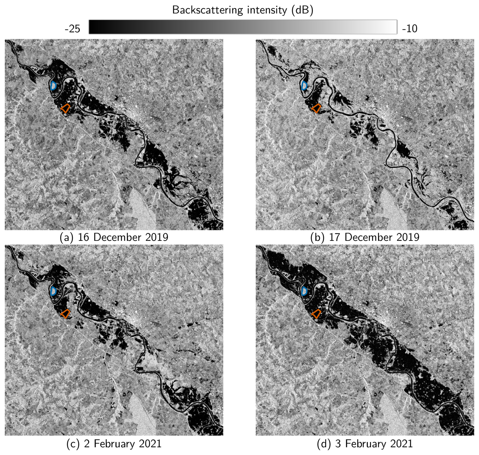
Figure 6 Four raw Sentinel-1 images in VH polarization of the 2019 and 2021 flood events on the Garonne River in France. The blue and orange polygons are used for the Equivalent Number of Looks computation.

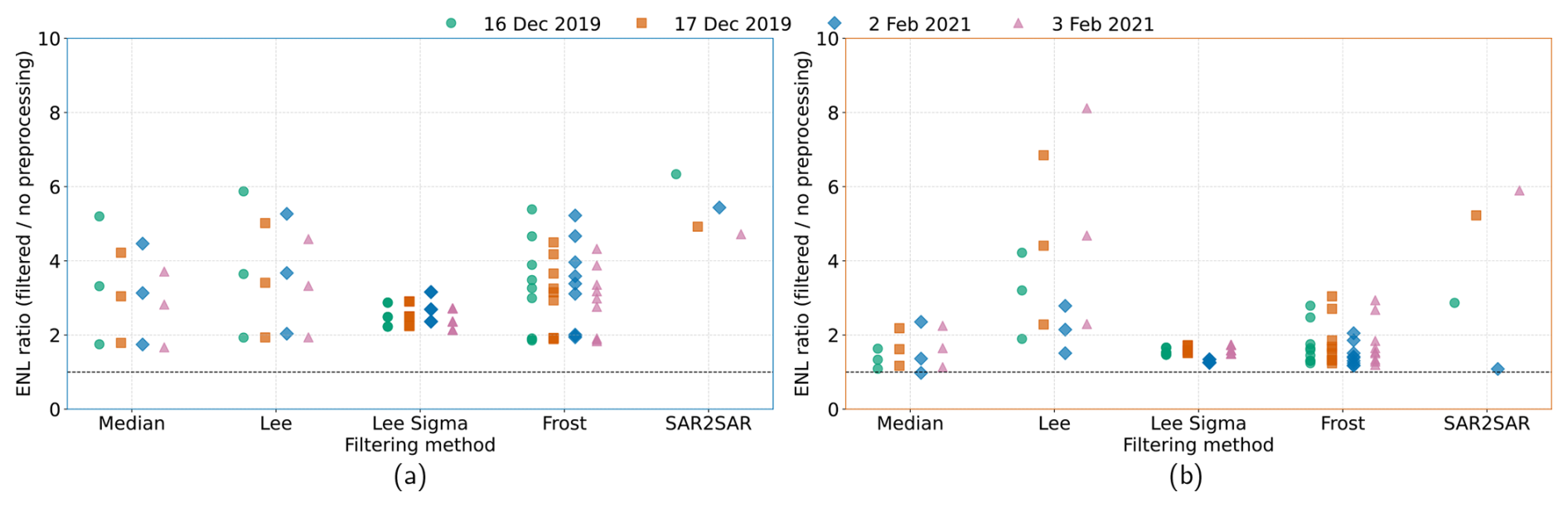
Figure 7 Equivalent Number of Looks (ENL) ratio (between images with and without preprocessing) for the four satellite images with different preprocessing for the dry homogeneous area (a) and flooded homogeneous area (b).

The quantitative analysis of edge and structure preservation is difficult because fine structures are close to the speckle noise spatial resolution (Lee et al., 1994). Edge preservation was not quantitatively evaluated in this study. The SAR2SAR approach gave the best quantitative results on noise reduction in homogeneous areas while visually preserving edges and structures. Traditional filtering methods had similar ENL values for some hyperparameter settings, showing their potential to reduce speckle noise but at the cost of preserving details (edge blurring) and the need for hyperparameter tuning.

Speckle reduction aims to improve the interpretability of the images and the extraction of information. Thus, the role of speckle reduction is analyzed in more detail in Sects. 4 and 5 to show its impact on interpreting SAR images and how the variability in speckle reduction changes the output.

4 Flood mapping

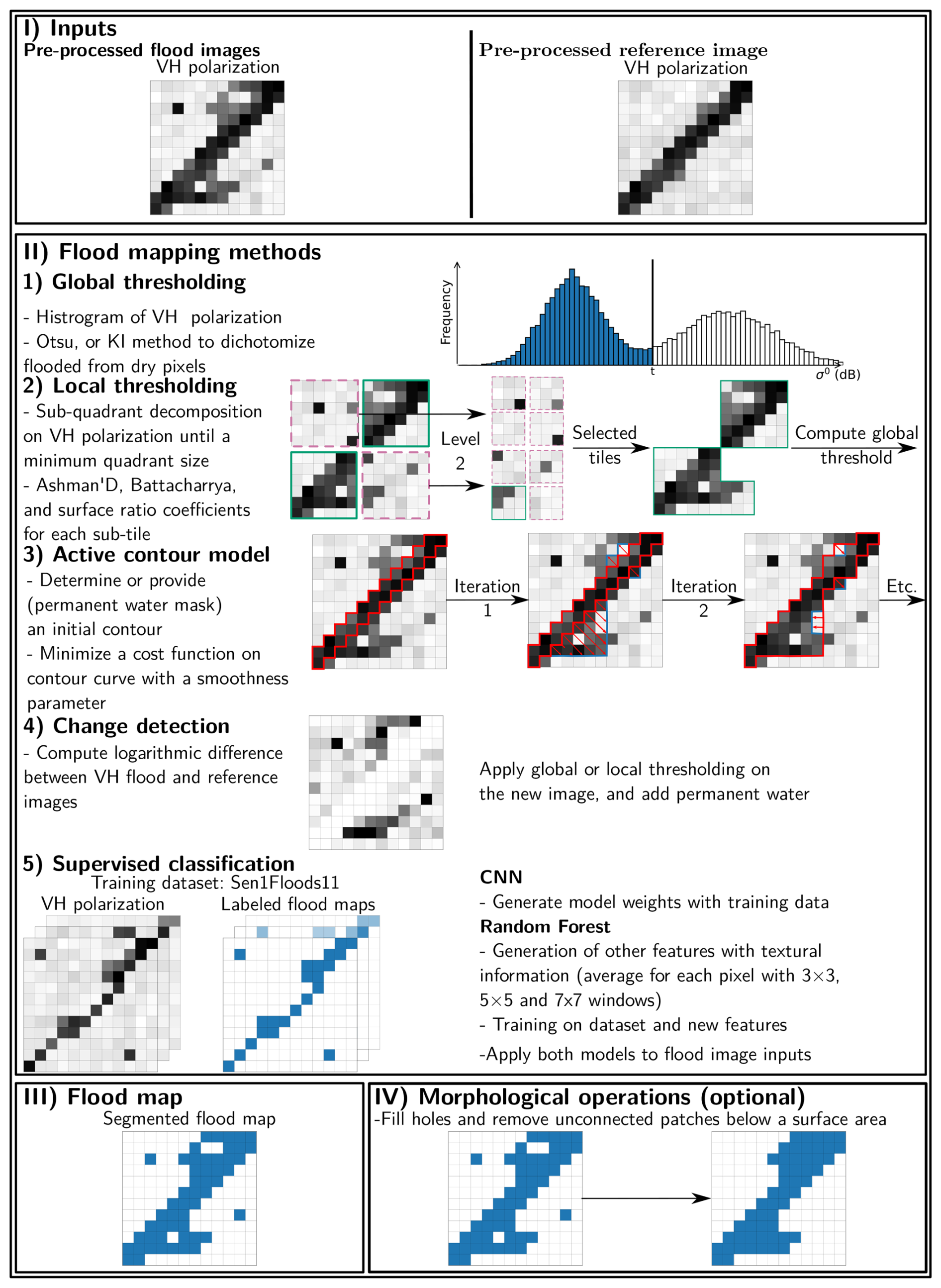
In this study, we generated an ensemble of flood maps by applying several flood mapping methods. The methodology for flood map generation is illustrated in Fig. 8, and follows this general workflow:

1. Input: Preprocessed SAR images.

2. Method selection: Global thresholding, local thresholding, active contour models, change detection, or supervised classification (Convolutional Neural Networks, Random Forest). Each method is evaluated over a range of hyperparameters (see Table 1). For instance, two methods for evaluating the threshold parameter are tested for global thresholding.

3. Flood map generation: Each parameter configuration results in a flood map $O\in \mathit{\{}\mathrm{0},\mathrm{1}{\mathit{\}}}^{N_x\times N_y}$.

4. Post-processing (optional): Morphological operations are applied on the flood maps to fill small holes and remove small elements not connected to the flood.

Figure 8 Schematic overview of the flood mapping methodology.

4.1 Methods

4.1.1 Global thresholding

Global thresholding of SAR images is a straightforward method to separate foreground (e.g., flooded pixels) from background (e.g., dry pixels) widely used in flood mapping for their simplicity (Martinis et al., 2009; Schumann et al., 2010; Pulvirenti et al., 2013). This approach assumes that the two-pixel classes (e.g., flooded and dry pixels) can be separated with a threshold value for the whole image. The threshold value is usually determined automatically (Sezgin and Sankur, 2004).

In this study, we evaluated the impact on the flood mapping of two widely used global thresholding methods: Otsu's method (Otsu, 1979) and the Kittler and Illingworth (KI) method (Kittler and Illingworth, 1986). Complementary details on both methods are provided in Appendix A1.

4.1.2 Local thresholding

Global thresholding assumes that the histogram is bimodal, which may not hold when the number of flooded pixels is low or due to spatial variability in backscatter caused by terrain or surface conditions across the image. To address this limitation, local-based thresholding was introduced (Martinis et al., 2015a; Twele et al., 2016; Chini et al., 2017). Images are divided into smaller tiles to identify bimodal histograms representing flooded and dry classes. From these identified sub-tiles, a threshold is computed with global thresholding. Following Chini et al. (2017), we used quad-tree decomposition to recursively split the image until reaching a minimum tile size (to guarantee statistical representativeness). A tile is eligible for thresholding if its histogram is bimodal, the distributions are normally distributed, and both classes are sufficiently represented. These conditions are evaluated by computing three qualitative coefficients (Ashman D, surface ratio, Bhattacharyya) described in Appendix A2.

This study evaluated the impact on the flood mapping of the minimum tile size and of the three coefficients for different values reported in Table 1.

4.1.3 Active contour models

A classical active contour model is based on the Chan-Vese segmentation method (Chan and Vese, 2001), which is inspired by the Mumford–Shah model (Mumford and Shah, 1989). This approach determines a contour C that segments the image into two regions so that the pixel intensities are approximately constant within each region. The segmentation problem is formulated as the following minimization:

$$\begin{array}{}\text{(14)}& \begin{array}{rl}& \underset{C}{min}\mathit{\alpha }\text{Length}\left(C\right)+\mathit{\nu }\text{Area}\left(\text{inside}\right(C\left)\right)+{\mathit{\lambda }}_{\mathrm{1}}\sum _{(i,j)\in \text{inside}\left(C\right)}\\ & {\left({\widehat{R}}_{i,j}-c_{\mathrm{1}}\right)}^{\mathrm{2}}+{\mathit{\lambda }}_{\mathrm{2}}\sum _{(i,j)\in \text{outside}\left(C\right)}{\left({\widehat{R}}_{i,j}-c_{\mathrm{2}}\right)}^{\mathrm{2}},\end{array}\end{array}$$

where α≥0 controls the smoothness of the contour, ν≥0 penalizes the area inside the contour, ${\mathit{\lambda }}_{\mathrm{1}},{\mathit{\lambda }}_{\mathrm{2}}>\mathrm{0}$ are weighting the data fidelity inside and outside the contour, respectively, and c₁ and c₂ are the average intensities inside and outside the contour C, respectively. The algorithm is adapted so that c₁<c₂, forcing flooded pixels with lower backscattering to be inside C.

In this study, we considered α as a hyperparameter, while the remaining parameters were fixed to λ₁=2, λ₂=1, and ν=0 for computational cost reasons. We chose to constrain the problem with λ₁>λ₂ to favor the identification of regions with lower mean intensities (typically associated with flooded areas in SAR imagery) as the foreground while assigning higher-intensity regions to the background. Active contour models require an initial contour as a starting condition for the segmentation process. Horritt (1999) suggests selecting the initial contour manually. In this study, the contour was initialized using a map of permanent water bodies from the Global Flood Monitoring Service with a 10 m resolution (https://global-flood.emergency.copernicus.eu/, last access: 26 May 2026) (Martinis et al., 2022).

4.1.4 Change detection

Change detection methods require at least two satellite images of the same area, one during the flood and the others before or after the event. The output of change detection methods depends on the reference image without floods, so the reference image should be chosen carefully (Hostache et al., 2012). Although there are methods using a stack of images (Clement et al., 2018), we focused on a pair of images. First, we computed the logarithmic difference between the two images because of the multiplicative character of speckle noise (see Eq. 5) (Bazi et al., 2005). Flooded pixels are then classified using global thresholding described in Sect. 4.1.1 with consistent parameter sampling. Similarly to global thresholding, the hyperparameter in the change detection method is the method to find the threshold on the image (Otsu or KI).

4.1.5 Supervised classification

Two supervised classification methods, widely used for flood mapping based on labeled training data (Zhao et al., 2021; Bentivoglio et al., 2022) are used in this work: Random Forests (RF) (Breiman, 2001) and Convolutional Neural Networks (CNN) (LeCun et al., 2015). For the RF approach, the pixel intensity is used as a feature. With only one band (VH polarization), the prediction capability of RF is limited. We added textural information by providing the mean value of each pixel with window sizes of 3×3, 5×5, and 7×7 pixels, resulting in four features.

Both models are trained with the Sen1Floods11 dataset (Bonafilia et al., 2020) (including 11 flood events with various geographic conditions) using VH polarization band and hand-labeled data dichotomizing flooded from dry regions. The trained model weights were used to generate flood maps from satellite imagery based on pixels' backscattering intensity. For reproducibility, the weights of both models are available at: https://github.com/jtravert/sar-flood-evaluation-framework/tree/main/sources/1_FloodExtent/methods/MLweights (last access: 26 May 2026). The training procedure for the CNN was adapted from Bonafilia et al. (2020) using a Fully-Convolutional Network model with a ResNet-50 backbone. The Random Forest classifier was trained for various numbers of estimators, maximum depth, and minimum leaf number with Bayesian optimization using the Optuna Python library (Akiba et al., 2019) (https://pypi.org/project/optuna/, last access: 26 May 2026). For supervised classification methods, no hyperparameters are considered, as their hyperparameters were optimized during the training procedure using Bayesian inference.

4.2 Post-processing of flood maps

After applying flood mapping methods, the flood maps can still contain artifacts caused by measurement noise, speckle, or processing errors. To improve the spatial coherence of flood maps, morphological operations (standard methods used in image processing) can be used to refine the flood maps. These operations include hole filling, which fills small gaps within flooded regions, and removal of isolated patches not physically connected to the flooded areas.

In this study, the influence of these operations was studied for holes and small patches of water from 1000 to 10 000 m². We applied morphological operations by filling holes of less than 10, 50, or 100 px and removing unconnected patches of less than 10, 50, or 100 px, representing nine configurations. The number of filled/removed pixels is the hyperparameter for morphological operations.

4.3 Results

Flood maps were generated using the five flood mapping methods with the hyperparameter settings detailed in Table 1. For each satellite acquisition, 1248 generated flood maps were produced (26 speckle filtering configurations ×48 flood mapping setups). These flood maps were optionally processed with morphological operations (nine configurations), resulting in 10 998 additional possible flood map variations for each satellite acquisition. In our implementation, the computation time for mapping a flood on a single preprocessed image was a few seconds for all methods, except for active contour, which required 5 to 10 min (depending on the smoothing hyperparameter), on Intel(R) Core(TM) i7-11850H @ 2.50 GHz processor. Each generated flood map was compared against hydrodynamic simulations, as described in Sect. 2.1.2. The evaluation process comparing observations to simulations focused on floodplain areas, excluding permanent water bodies and exclusion zones. The exclusion layer indicates areas where the satellite sensor cannot accurately discriminate flooded areas from dry areas due to water-look-alike conditions (e.g., roads, dikes, wetlands). The exclusion mask on the Garonne domain was retrieved from the Global Flood Monitoring service and the generation process is described in Wagner et al. (2026).

At the grid points, a hit occurs when a pixel is correctly predicted to be flooded (True Positive (TP)), and a correct rejection (True Negative (TN)) occurs when it is correctly predicted to be dry. A false alarm (False Positive (FP)) and a miss (False Negative (FN)) occur when a pixel is simulated as flooded or dry, respectively, whereas the opposite is observed. Two standard metrics for comparing flood maps (Hunter, 2005; Grimaldi et al., 2016) were used:

• Accuracy: Proportion of correctly predicted pixels (both flooded and non-flooded) relative to the total number of pixels:

  $$\begin{array}{}\text{(15)}& \mathrm{ACC}={\displaystyle \frac{\mathrm{TP}+\mathrm{TN}}{\mathrm{TP}+\mathrm{TN}+\mathrm{FP}+\mathrm{FN}}}.\end{array}$$

• F1-score: The F1-score is defined as:

  $$\begin{array}{}\text{(16)}& F\mathrm{1}={\displaystyle \frac{\mathrm{2}\cdot \mathrm{TP}}{\mathrm{2}\cdot \mathrm{TP}+\mathrm{FP}+\mathrm{FN}}}.\end{array}$$

Both metrics range from 0 to 1, with higher values indicating better performance. The flooded area in the evaluation zone is also computed to evaluate the variability of the flood map outputs.

4.3.1 Flood mapping methods evaluation

First, the images generated without applying morphological post-processing operations are analyzed. Figure 9 shows the variability of the Accuracy, F1-score and flooded area metrics across the four satellite acquisitions. Each box plot represents the range of metric variations of a flood mapping method due to varying input preprocessing and hyperparameter settings. For each method, box plots are displayed in different colors for the four satellite images. These box plots should be compared with one another for the same acquisition date to assess method performance variability under consistent conditions.

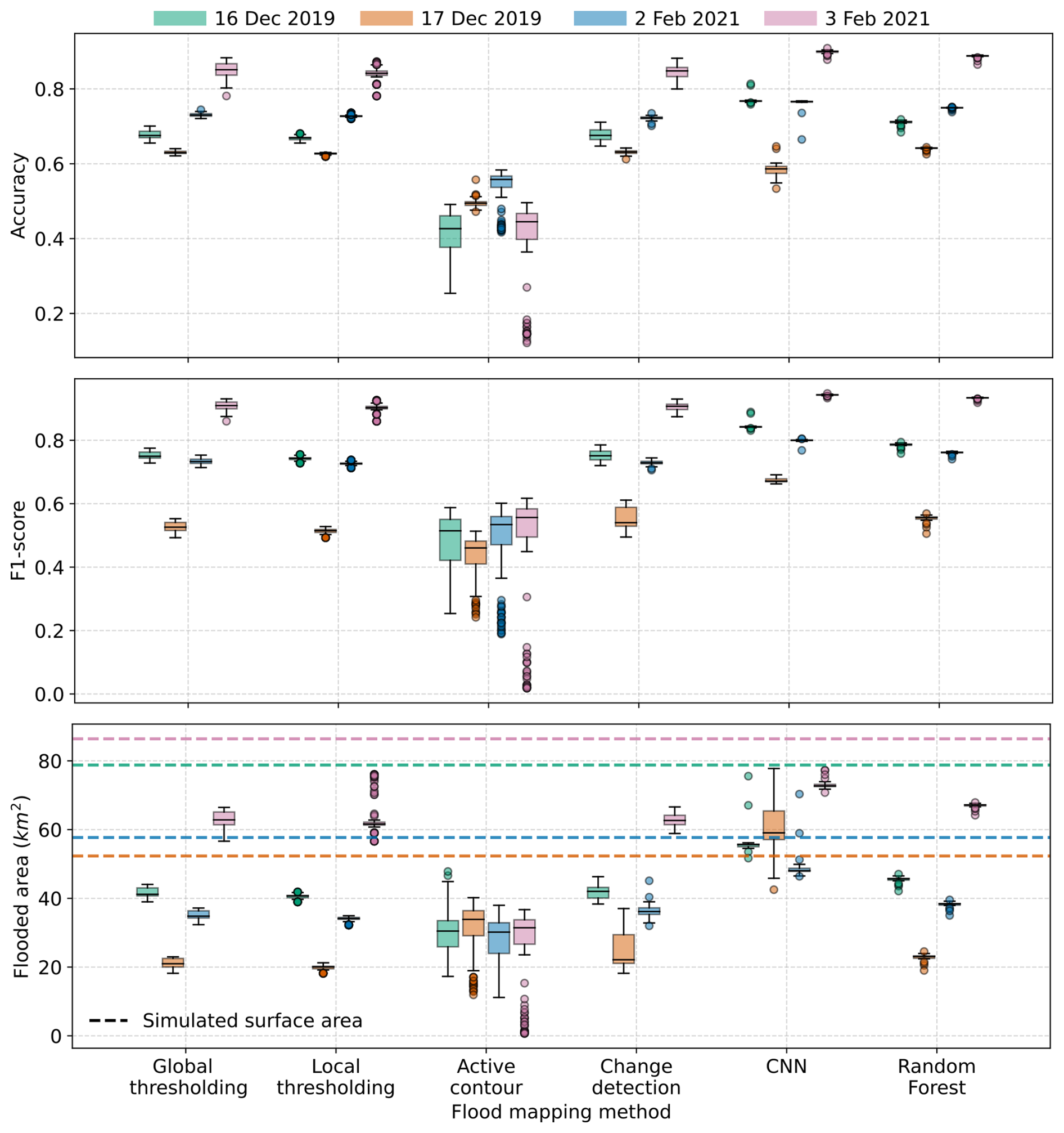
Figure 9 Accuracy, F1-score and flooded area for the generated flood maps for four satellite images and six flood mapping methods compared against their respective simulated flood maps.

The CNN approach presented the highest median performance (between 0.80 and 0.94 for F1-score) with a narrow inter-quartile range (<0.005) in three out of the four acquisition dates (except for 17 December 2019 acquisition). The Random Forest also performed well (F1-score median between 0.76 and 0.93), but with slightly lower scores and higher variability. Both supervised classification methods exhibit low variance because of the absence of hyperparameter tuning, leaving speckle filtering as the main source of variation. In contrast, active contour models exhibited larger variability in Accuracy and F1-score across all dates. It underlined the sensitivity to either the smoothing parameter (α) or image preprocessing. While they occasionally achieved reasonable performance for specific configurations, their inconsistency (e.g., F1-score inter quartile range between 0.27 and 0.38 on the 16 December 2019) makes them less reliable in operational settings. This method can work only after careful manual tuning, limiting its operational appeal. Active contour models are usually better for local scales and simple flood patterns around the initial contour. Thresholding methods (global and local) showed moderate performance and low variability. Additional configurations with a larger hyperparameter space showed that the thresholding methods were not very sensitive to their hyperparameters. For some configurations, local thresholding resulted in comparable metric values to supervised classification while being easy to use. Finally, change detection methods provided similar moderate results regarding F1-scores and Accuracy. Their variance was relatively low but was higher for some acquisition dates (17 December 2019 and slightly 3 February 2021), likely due to differences in magnitude change between the pre- and during-flood images, with smaller flood extent on 17 December 2019. The supervised classification method provided the best trade-off between accuracy and robustness. When training data or model weights are unavailable, local thresholding or change detection methods remain attractive because they require almost no user input and result in similar scores with appropriate tuning.

Figure 9 also displays the flooded area for all flood mapping methods and satellite acquisitions. In the evaluation zone, containing the simulation domain without the exclusion zones and the minor bed representing a total of 100.2 km², the simulated flooded areas were 78.78 km² (16 December 2019), 52.32 km² (17 December 2019), 57.70 km² (2 February 2021) and 86.41 km² (3 February 2021). CNN produced the largest flooded area estimates, with the smaller discrepancy to the simulated flooded area. In contrast, the other methods highly underestimated the flooded areas systematically relative to the simulations. In general, outputs from hydrodynamic models provide smooth flooded surface with hydraulic connectivity. On the contrary, for the generated flood maps from SAR imagery, floods in vegetated or urban areas or between the dikes are often not well detected which can cause an underestimation of the flooded area, and the flood extent is more segmented and less smooth. On the one hand the simulations are conservative and overestimate the flooded area while the extracted flood maps underestimate the flooded areas. However, the main goal should be to match the geometric pattern and have a similar flood map geometry between the simulations and the observations even if there are small holes in the observed flooded area. The estimated flooded area can differ by 20 to 30 km² between methods, highlighting significant differences in flood map extraction approaches. Additionally, for a given method, the impact of hyperparameters or input images can be significant, with variations of 5 to 10 km² for active contour or change detection and CNN for 17 December 2019.

4.3.2 Impact of preprocessing

In most flood studies, the preprocessing of speckle noise is often assumed to be deterministic, with only one method (usually the Lee or Lee Sigma filter) (Di Baldassarre et al., 2009; Landuyt et al., 2018); however, the influence of speckle filtering choice on flood mapping can be significant. The preprocessing strategies should be evaluated for fixed configurations (flood mapping method and hyperparameter) to study the impact of preprocessing alone. For instance, the effect of preprocessing for CNN-generated flood maps is reported in Fig. 10. It highlighted the impact of preprocessing with a highly variable flooded area for Median filtering, depending on the window size of the filter (the only parameter for the Median filter). With filtering, the flooded area is larger than that of images without preprocessing. Between the different preprocessing methods, the flooded area has important variations showing the impact of the preprocessing method on the generated flood maps.

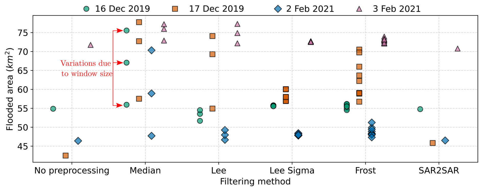
Figure 10 Impact of different filtering methods on the flooded area for flood maps generated using Convolutional Neural Networks.

Figure 10 illustrates the impact on the flooded area of the different filtering methods with a single flood mapping configuration. In total, Table 1 lists 48 configurations (2 for global thresholding and change detection, 36 for local thresholding, 6 for active contour, and one for each supervised classification method). For the Median, Lee, Lee Sigma, and Frost filters, we analyzed the impacts of their hyperparameters on these 48 configurations. The difference between the minimum and maximum value for each metric was calculated for every filter configuration (e.g., for the CNN configuration on 2 February 2021, the range of variation between the min and max values for the Median filter was 23 km²). Figure 11 presents the min-max variation in F1-score and flooded area due to speckle filtering hyperparameters for 2 February 2021. Each flood mapping configuration is visualized with a point with distinct markers for the different methods. The results indicate that the sensitivity to speckle filter hyperparameters varies by flood mapping method. For instance, the active contour method exhibits high sensitivity to the Median filter’s window size, with variations ranging from 4 to 16 km². In contrast, global and local thresholding methods exhibit minimal sensitivity, with variations of less than 1 km². Overall, the Lee Sigma filter exhibited the lowest variability across all configurations. Local thresholding, change detection, and Random Forest configurations are more sensitive to Lee filter or Frost filter hyperparameters than Lee Sigma or Median filters.

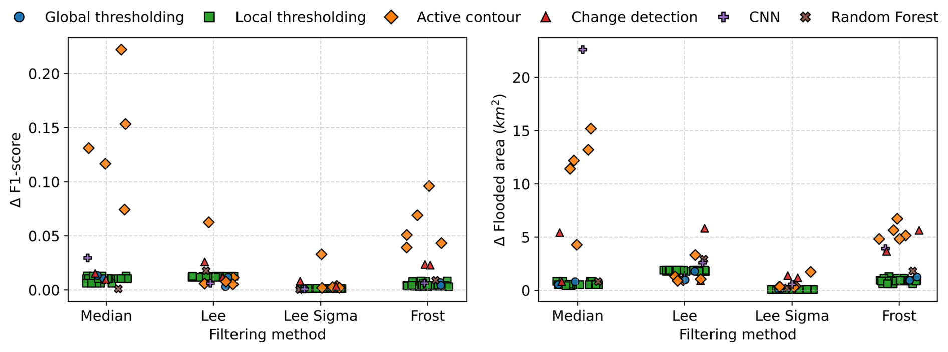
Figure 11 Range of variation (between the minimum and maximum values) of F1-score and flooded area due to filtering methods hyperparameters for the 48 flood mapping configurations for 2 February 2021 acquisition. The points are jittered horizontally for visualization purposes.

4.3.3 Impact of hyperparameters

The role of hyperparameters used in flood mapping methods was evaluated, excluding the supervised classification methods (CNN and Random Forest), for which no hyperparameters were defined in this study. Similarly to the preprocessing analysis, we fixed the preprocessing configuration to isolate and evaluate the impact of flood mapping hyperparameters.

The range of variability due to the hyperparameters of flood mapping methods for all 26 speckle filtering configurations (3 configurations for Median and Lee filters, nine configurations for Lee Sigma and Frost Filters, one configuration for SAR2SAR and no preprocessing) is evaluated. The results for the acquisition on 2 February 2021 are presented in Fig. 12.

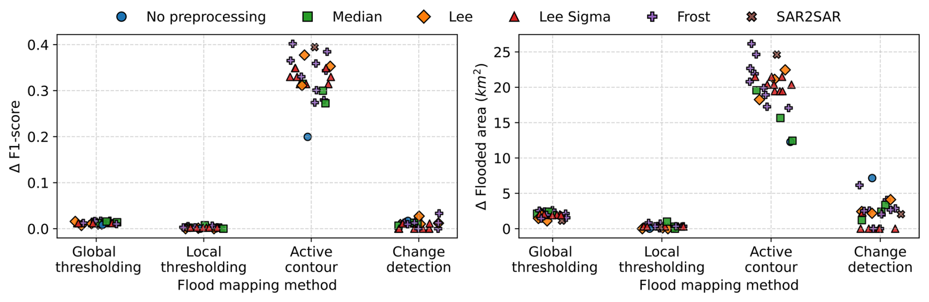
Figure 12 Range of variation (between the minimum and maximum values) of F1-score and flooded area due to flood mapping methods hyperparameters for the 26 speckle filtering configurations for 2 February 2021 acquisition. The points are jittered horizontally for visualization purposes.

In this study, the active contour method showed the highest sensitivity to flood mapping hyperparameter variations, with F1-score differences reaching up to 0.4 and differences in flooded areas ranging between 15 and 25 km² for all speckle filtering configurations. In contrast, change detection and local thresholding methods demonstrated low sensitivity, with F1-score differences of less than 0.03 and flooded area variations limited to a few square kilometers. For active contour models, most of the variability can be attributed to the flood mapping hyperparameters. While thresholding methods showed limited variability, both active contour and change detection methods displayed greater sensitivity depending on the fixed speckle filtering configuration. For instance, variations in F1-score or flooded area due to hyperparameters for change detection were smaller for Lee Sigma configurations compared to Median filtering configurations.

4.3.4 Impact of morphological operations

Figure 13 shows the improvement or degradation in the F1-score for global thresholding, local thresholding, and change detection methods for one of the acquisitions (2 February 2021) when using morphological operations. The color intensity represents the average gain (or loss) relative to the configurations without morphological post-processing. The active contour and supervised classification approaches are not reported here, as morphological operations had negligible or no effect on the generated flood maps due to the minimal presence of holes or small unconnected flood elements in these flood maps.

We observed that the F1-score increased for the three methods, especially for large hole filling (50 to 100 px) and small patch removal (10 to 50 px). This is likely due to eliminating isolated false positives and filling small gaps, improving the spatial coherence of flood maps. However, with the increasing size of patch removal, the performance decreases, suggesting that the small-scale features are well-captured and should not be removed. While the morphological operations improved the statistics for the F1-score, the physical representation of the flood may not be improved, with for instance flooded regions on small hills when using filling operations.

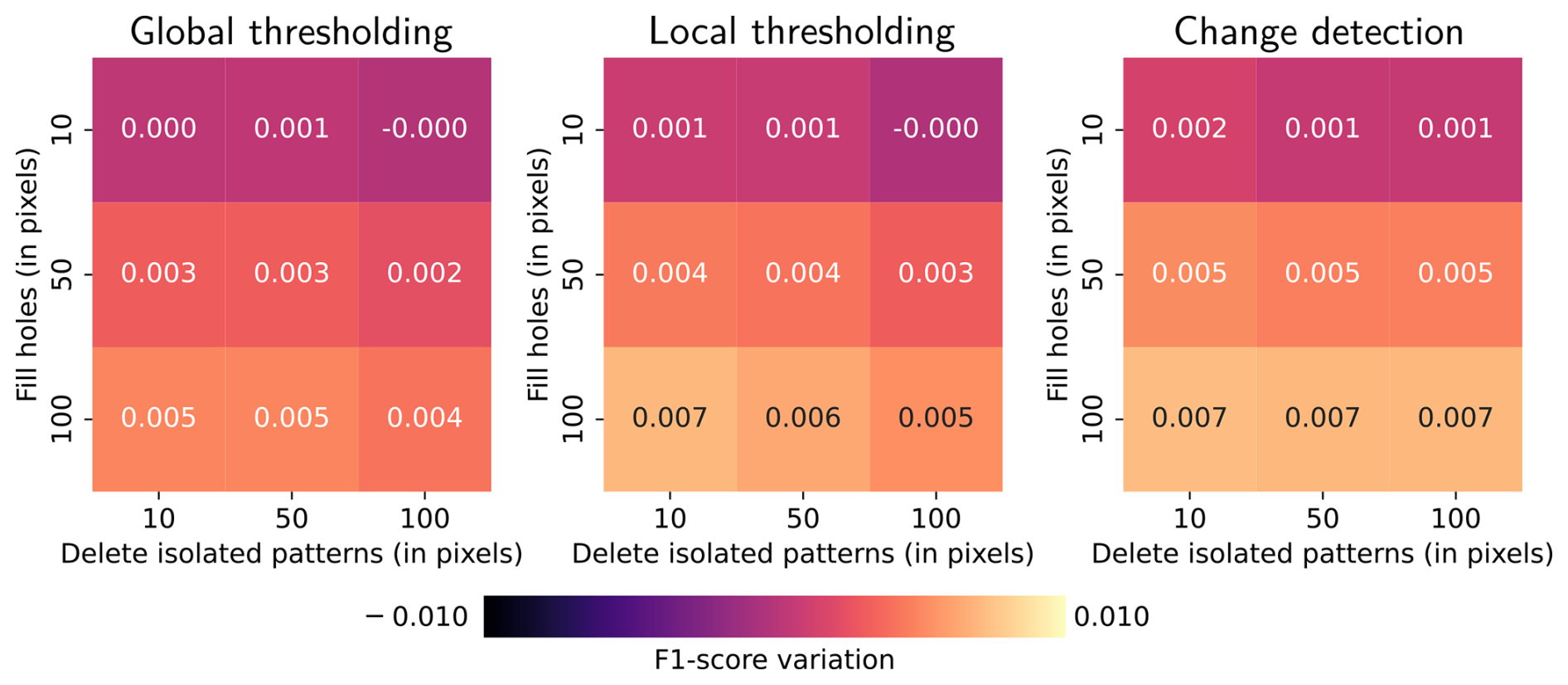
Figure 13 Heatmaps representing the average gain (or loss) in F1-score due to morphological operations relative to configurations without morphological post-processing.

Finally, Fig. 14 compares the flood maps with the highest F1-scores obtained for each method, including those enhanced with morphological operations for 2 February 2021. The CNN-based approach achieved the best overall performance, with an F1-score of 0.769, followed by the Change Detection and Random Forest methods. The flood map produced by the CNN is the most continuous but tends to overestimate the flooded area. The active contour model also exhibits a continuous flood extent, but it significantly underestimates inundation in both the upstream and downstream regions. The other methods result in less smoothed flood extent, capturing more localized details and irregularities. While some of these details may correspond to actual observations, their fragmented nature results in poorer alignment with the continuous structure of the simulated flood map, while having patterns that match the simulated flood map closer than for CNN.

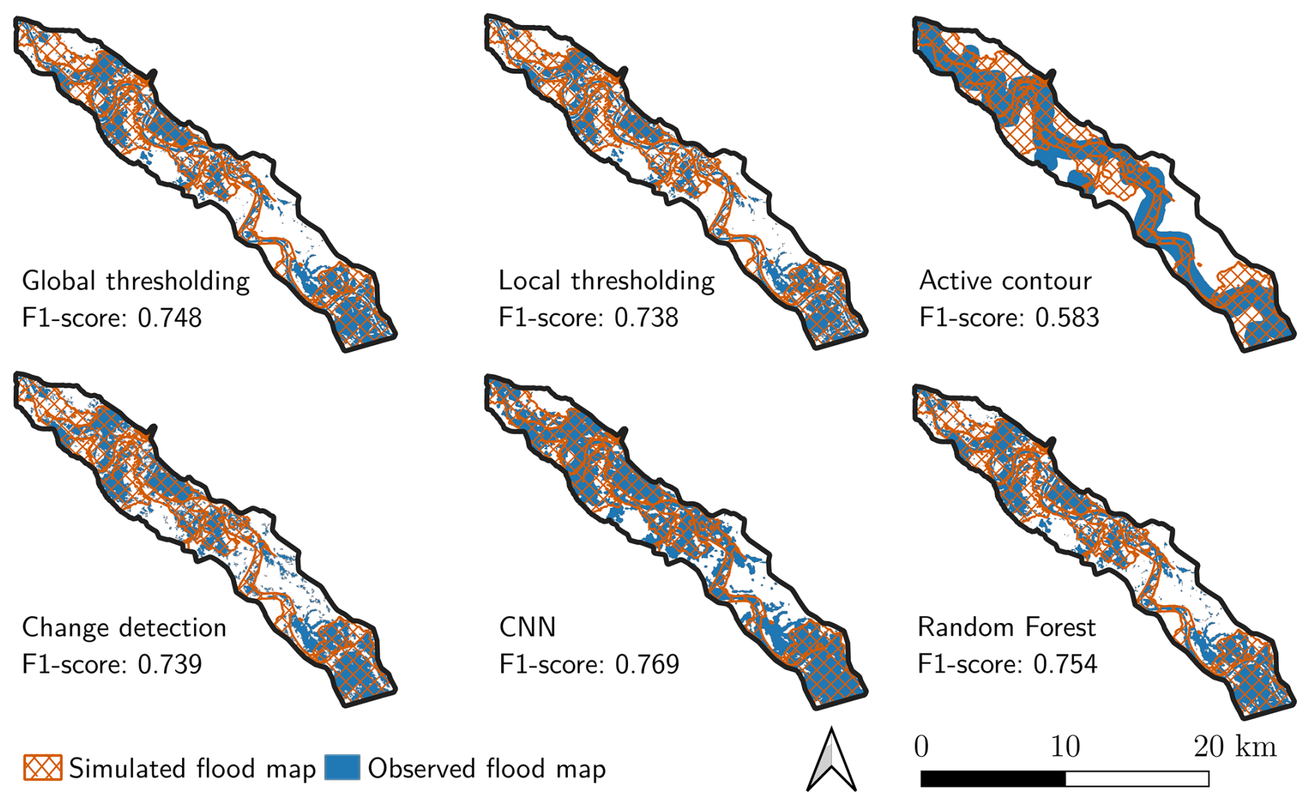
Figure 14 Comparison of the simulated flood maps (orange) with the generated flood maps (blue) for 2 February 2021.

5 Water depth estimation

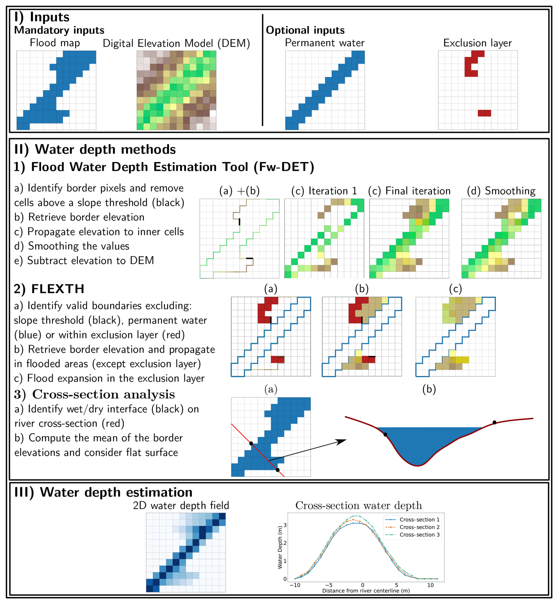
The flood maps extracted from the preprocessed SAR images can be used with Digital Elevation Models (DEM) including the bathymetry of the river channel, to construct water depth fields. In the literature, the approach of Hostache et al. (2009) for water depth estimation has proved effective but requires prior expertise in the flow motions and extensive fieldwork to constrain the method. In this study, we preferred to compare automatic water depth estimation methods on the whole flood map or specific cross sections. Methods such as the Flood Water Depth Estimation Tool (Fw-DET) (Cohen et al., 2018) or the FLEXTH methodology (Betterle and Salamon, 2024) are available to derive water depth fields across the entire domain based on a flood map and DEM. Other methods rely on cross-section analysis by considering that the free surface is flat on a cross-section, thus retrieving the water depth field by knowing the locations of the edges of the flood and topography. We generated water depth fields by applying these methods across a range of hyperparameters, as summarized in Table 1. The water depth estimation workflow follows a structured sequence illustrated in Fig. 15:

1. Input: Flood maps derived from SAR imagery and a Digital Elevation Model (DEM), all projected on the same spatial grid. The DEM is a combination of topographic data at 1 m spatial resolution with vertical accuracy between 0.2 and 0.5 m, and the bathymetry of the channel (based on 70 cross-sections measurements).

2. Methods: Fw-DET, FLEXTH, or cross-section analysis. Each method is evaluated for different hyperparameters (see Table 1).

3. Water depth estimation: Each method determines the water surface elevation and subtracts the underlying terrain elevation from the DEM to generate a water depth field.

Figure 15 Schematic overview of the water depth estimation methodology.

5.1 Methods

5.1.1 Fw-DET method

The Flood Water Depth Estimation Tool (Fw-DET) (Cohen et al., 2018, 2019) quantifies water depth continuously in the domain using a flood extent polygon and a Digital Elevation Model. A schematic representation of Fw-DET principle is presented in Fig. 15II(1). Flood boundaries are derived from the flood map and converted into a line layer, while steep slope cells are filtered out using a slope threshold. This line layer is rasterized to align with the DEM grid. Elevation values are extracted for these boundary cells, and each cell within the flood extent polygon is assigned the elevation of the nearest boundary cell under the assumption of a flat water surface. Water depth is computed by subtracting the DEM elevation from the water surface elevation. To mitigate artifacts caused by mismatches between the DEM and the flood extent, a smoothing procedure is applied multiple times using a 3×3 window.

This study considered the number of smoothing iterations and the slope threshold as hyperparameters. The latest version of the code developed by Cohen et al. (2019) is available at https://github.com/csdms-contrib/fwdet (last access: 26 May 2026). For the present study, the code was adapted to operate without the QGIS interface, using standalone Python scripts to enable batch processing.

5.1.2 FLEXTH method

The FLEXTH method (Betterle and Salamon, 2024) presents an approach similar to the Fw-DET methodology but introduces improvements to mitigate unrealistic water depth estimates (Cohen et al., 2019). Figure 15II(2), depicts the FLEXTH methodology schematically. The methodology was extended to account for additional inputs, such as exclusion or permanent/seasonal water body masks. The method expands the flooded area into adjacent no-data regions and estimates the water depths based on the DEM (Betterle and Salamon, 2024). As in Fw-DET, pixels along the flood boundaries with a slope exceeding a user-defined threshold are excluded from the boundary. Water depths within the flooded area are then estimated using a weighted average of the boundary cell elevations based on the closest cells up to a specified maximum number of neighbors.

The slope threshold and the maximum number of neighbors used in the computation were considered hyperparameters. In Betterle and Salamon (2024), they highlighted that these two parameters are the most influential in the FLEXTH method. The FLEXTH method, initially developed by Betterle and Salamon (2024), is available as a Python code at https://code.europa.eu/floods/floods-river/flexth (last access: 26 May 2026) and was adapted for the needs of our study.

5.2 Cross-section approach

The two previous methods estimated the water depths continuously across the domain. An alternative approach is to perform cross-section analysis along the river channel by extracting the surface elevation at the dry/flood interface along predefined cross-sections. The water surface is assumed to be flat for each cross-section, and its elevation is computed as the mean elevation of the identified boundary cells. However, this method is sensitive to errors caused by over-detection of the wet/dry interface along the cross-sections. To address this issue, an alternative strategy involves considering only the left and right banks of the flood extent (Schumann et al., 2007), excluding other points within the flooded area. This strategy is displayed schematically in Fig. 15II(3). In this study, we tested this second approach. The cross-section approach did not use any hyperparameters in this study.

5.3 Results

The methods for estimating water depth fields were applied to the flood maps generated in Sect. 4. For each satellite acquisition, more than 10 000 flood maps were generated. In our implementation, the processing time to generate the water depth field for each flood map was approximately 15 s for Fw-DET, 30 s to 1 min for FLEXTH, and a few seconds for the cross-section approach. All computations were conducted on an Intel® Core™ i7-11850H CPU @ 2.50 GHz. Thus, generating water depth fields for all hyperparameter combinations (nine configurations of the Fw-DET method, nine configurations of the FLEXTH method, and one for the cross-section approach) would result in an impractically large number of outputs and computation time. Since the generation of water depth fields depends on the input flood contour, our focus is on analyzing the variations of the water depth fields due to variations in the flood contour (due to speckle filtering, flood mapping methods, and hyperparameters used previously). We selected 10 flood maps per flood mapping method to capture a representative range of potential flood map inputs. These were sampled uniformly across the full span of their F1-scores, from the lowest to the highest score, to ensure coverage of both high- and low-quality segmentation results. The Fw-DET, FLEXTH, and cross-section methods were applied for these flood maps. For the cross-section approach, the results were analyzed for two user-defined cross-sections shown in Fig. 16. The estimated water depths were compared with the hydrodynamic simulations and watermarks presented in Sect. 2.1.2. The watermarks were used only for the 16 December 2019 and 3 February 2021 acquisitions (near the flood's peak). For the comparison against simulations, the Root Mean Square Error (RMSE) was computed, comparing pixel-to-pixel values. The rasterized results were projected at the measurements' locations for the watermarks. Here, contrary to the flood mapping evaluation, all the domain is taken into account including the minor bed and the exclusion zones since the three water depth estimation methods aim to estimate the water depth even in exclusion zones with specific behaviors (e.g., propagation of the water in the exclusion zone with the FLEXTH method, or with the cross-section method which considers a flat water surface between the two edges).

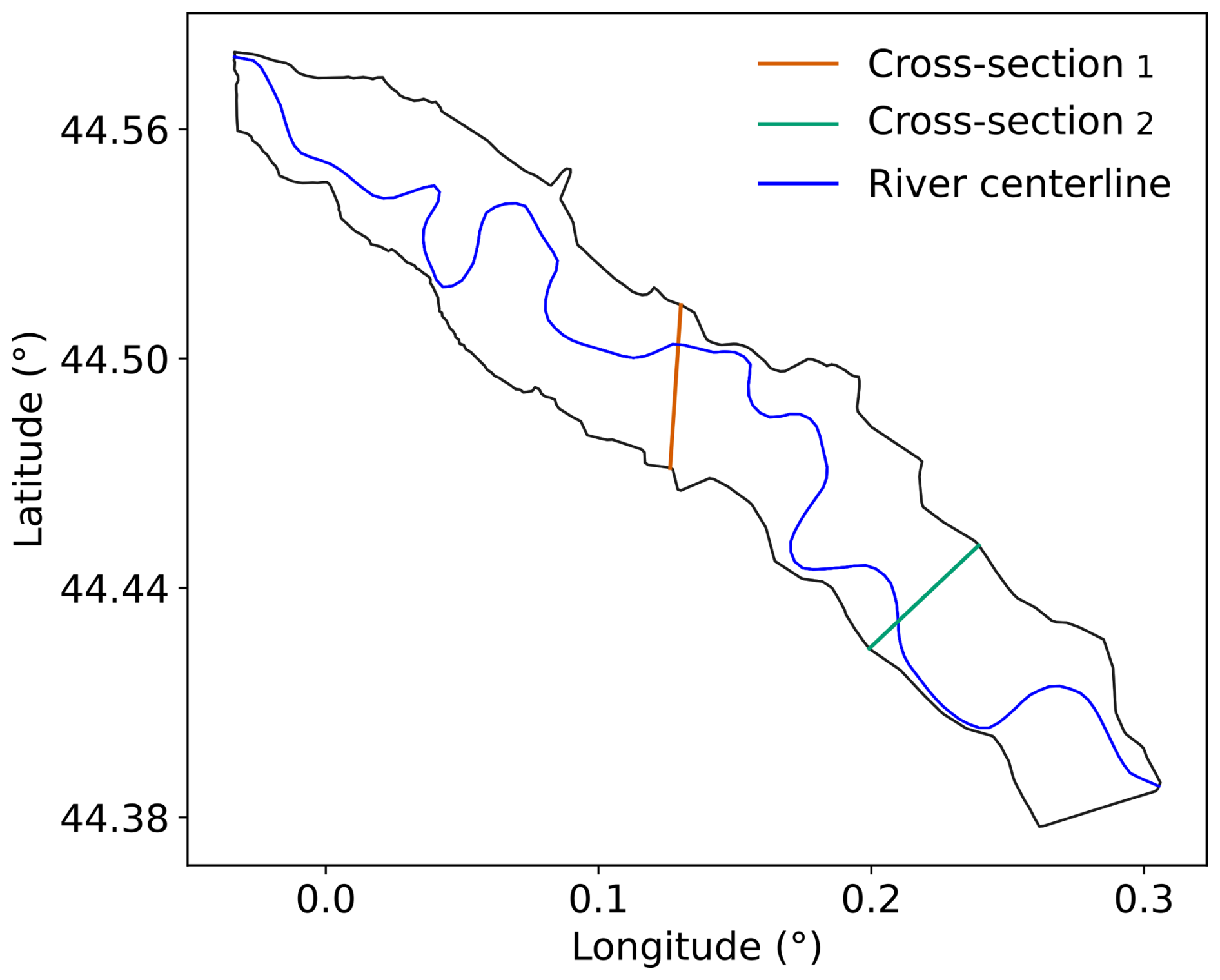
Figure 16 Visualization of the two cross-sections (cross-section 1 in orange and cross-section 2 in green) used in the study.

5.3.1 Water depth estimation methods evaluation

Figure 17 shows the RMSE of the estimated water depths compared to hydrodynamic simulations (see Fig. 17a) and watermarks (see Fig. 17) for the Fw-DET and FLEXTH methods. Each box plot indicates the variability explained by the input flood map or water depth estimation hyperparameters.

FLEXTH and Fw-DET demonstrate comparable performance in terms of median RMSE. Both methods exhibit a median RMSE ranging from 0.8 to 1.9 m, depending on the satellite image acquisition. The variability of the RMSE is also comparable for both algorithms, with slightly more outliers for the FLEXTH method, which may be caused by the used hyperparameter values. These conclusions are similar either with the simulated water depth fields or watermarks as validation dataset. For the watermarks, the variability is more important. The observed variability and elevated RMSE values can be attributed to the flood map selection from previous processing steps, including high and low F1-score maps relative to the reference. This variability and the influence of water depth estimation method hyperparameters are further analyzed in Sect. 5.3.2 for the Fw-DET and FLEXTH methods.

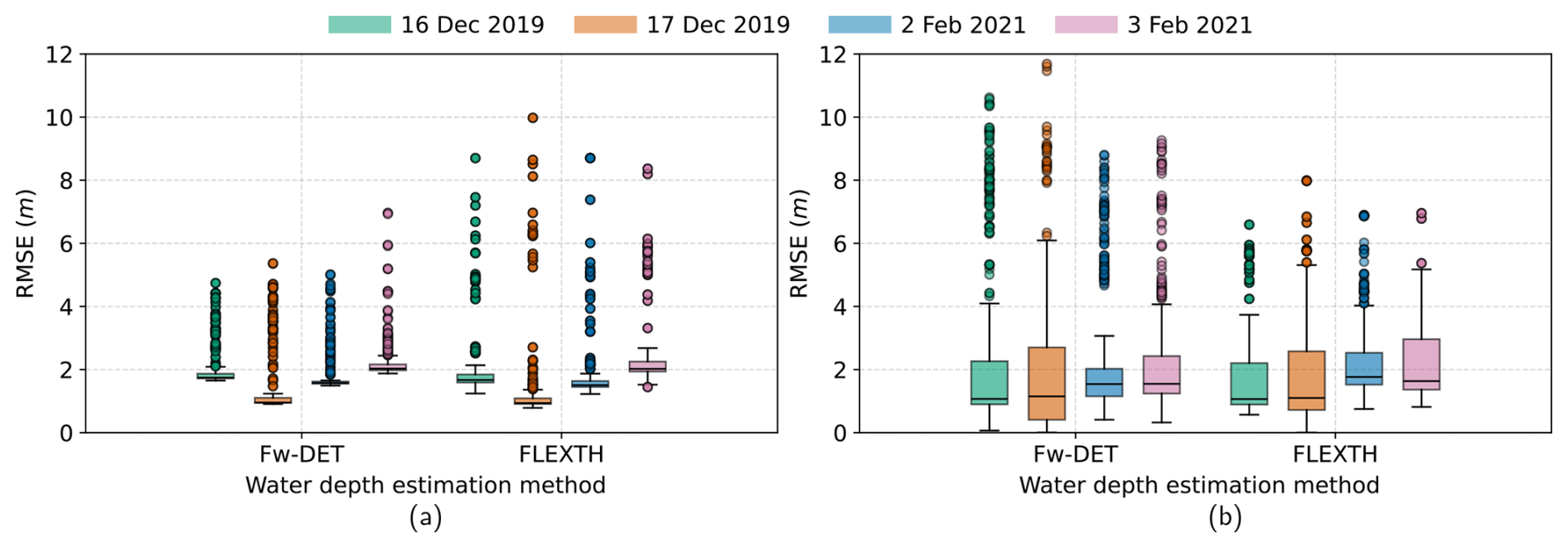
Figure 17 Root Mean Square Error (RMSE) between the estimated water depths and simulated (a) or watermarks (b) for Fw-DET and FLEXTH methods for four satellite images.

Next, Fig. 18 presents the RMSE of water depth estimates on the two selected cross-sections (see Fig. 16) for the cross-section approach, along with Fw-DET and FLEXTH methods projected onto these cross-sections.

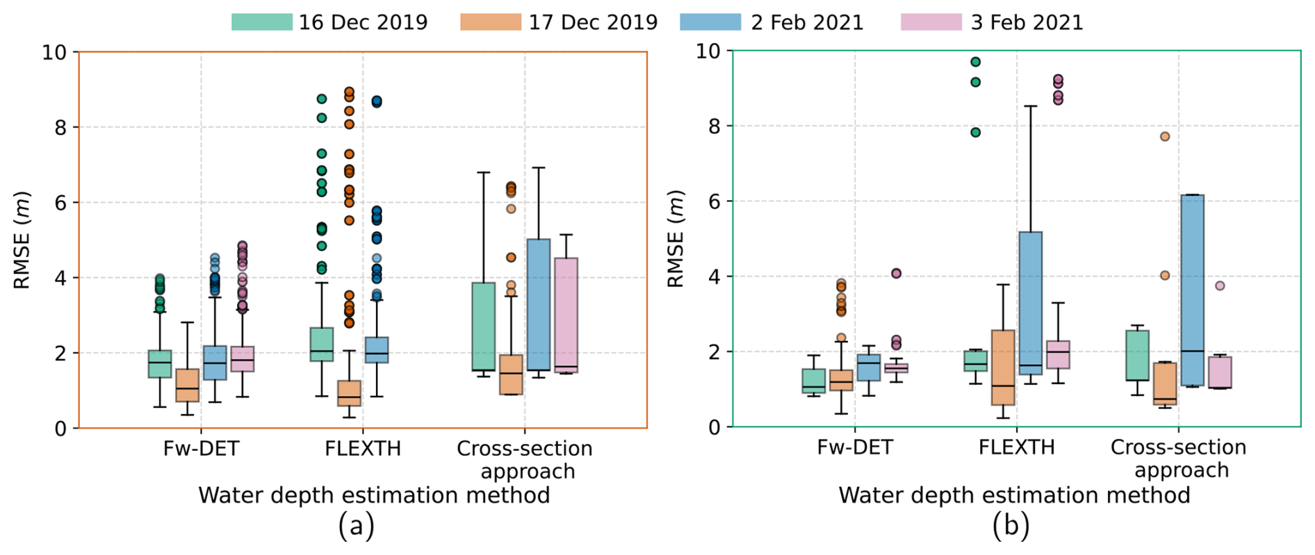
Figure 18 Comparison of Fw-DET, FLEXTH, and cross-section approaches on cross-section 1 (a) and cross-section 2 (b) for four satellite acquisitions against hydrodynamic simulations.

The Fw-DET and FLEXTH methods exhibited similar RMSE performance for both cross-sections, though FLEXTH showed higher variability. The cross-section approach, while showing similar or slightly higher median RMSE values compared to FLEXTH and Fw-DET on the two cross-sections, exhibited more variability, particularly for the 2 February 2021 image, which was likely related to challenging flood contour detection conditions for that image. The Fw-DET and FLEXTH algorithms propagate the surface elevation from the edges of the flood to the inner flood. The cross-section approach, on the other hand, relies only on the identification of the right and left edges of the flood. Then, the cross-section approach is highly sensitive to identifying the border of the flood on the cross-section, while it is less the case for Fw-DET and FLEXTH, which rely on the whole flood extent borders. The variability of the RMSE for the cross-section approach was entirely due to the variability of the input flood maps, since the cross-section approach was considered without hyperparameters.

5.3.2 Impact of hyperparameters and flood map inputs

The influence of flood map inputs and method hyperparameters on water depth estimation performance was evaluated for the Fw-DET and FLEXTH methods. Figure 19 presents the distribution of RMSE values, computed against hydrodynamic simulations across four satellite acquisitions, grouped by flood mapping method used as input to the water depth estimation methodology.

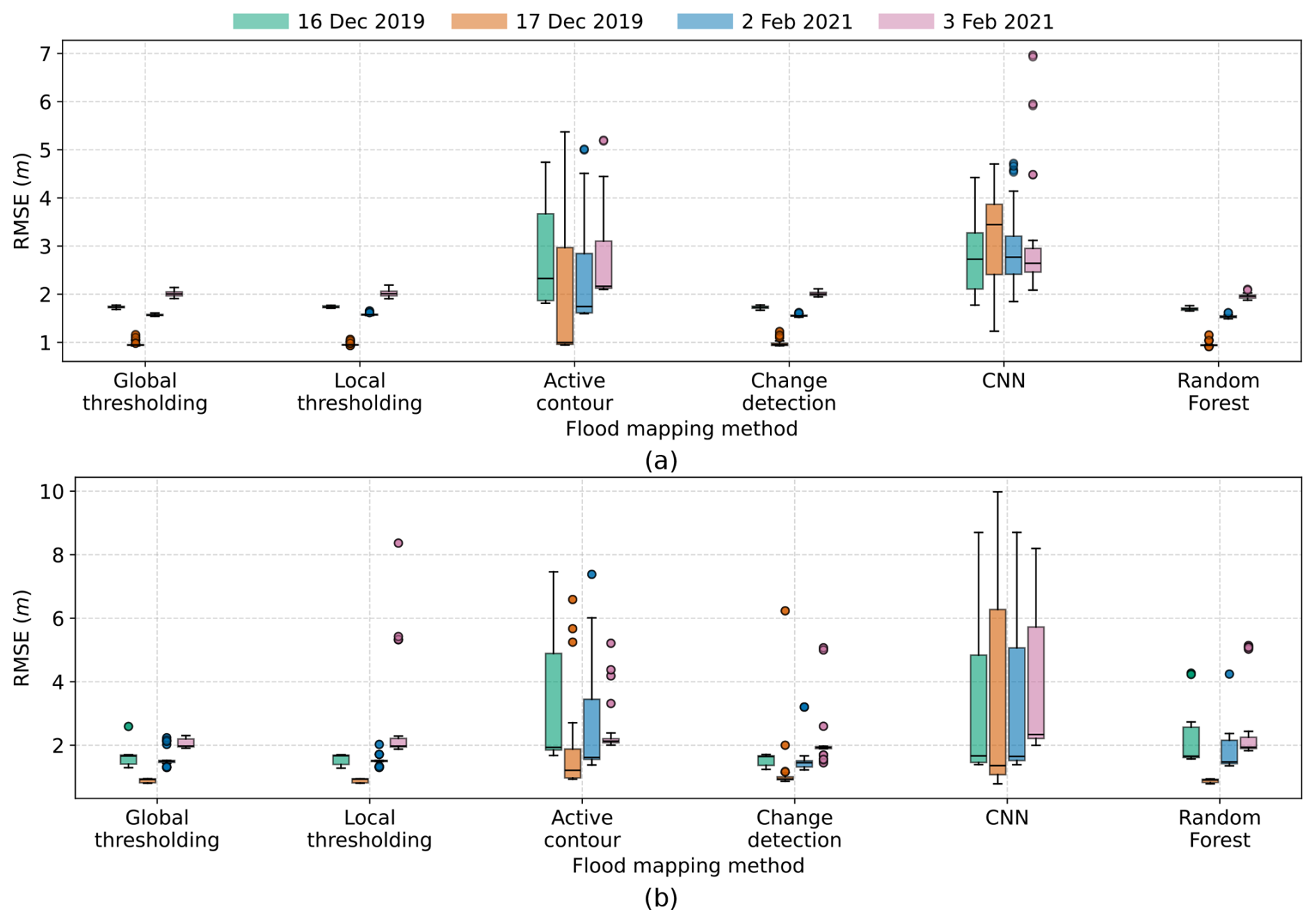
Figure 19 Impact of the flood mapping method used for water depth estimation for the Fw-DET method (a) and FLEXTH method (b) across four satellite acquisitions.

The results indicated that the flood map used as input for the water depth estimation process significantly influenced the estimation accuracy. Flood maps derived from global and local thresholding yielded lower RMSE and variability. In contrast, flood maps produced with CNN and active contour models lead to greater variability and higher RMSE in water depth estimates. However, the median RMSE values for CNN and active contour flood mapping methods are close to the other algorithms, suggesting that they can achieve comparable or better results with water depth estimation method parameter tuning. The outputs from CNN and active contour models are smoother, but their ability to precisely delineate flood boundaries is reduced due to the smoothness. This can result in significant errors in water depth estimates, particularly in areas with steep terrain. Furthermore, the large RMSE for the CNN method suggests that the extracted flooded surface is physically wrong on these cross-sections. The tendency of the CNN to overestimate the flood extent size leads to water edges in high topography gradient leading to important errors in the water depth estimation.

To study the influence of hyperparameters in the FLEXTH and Fw-DET methodologies, we proceeded similarly as in Sect. 4.3.3 for flood mapping methods. For each hyperparameter configuration (9 each for FLEXTH and Fw-DET) of water depth estimation methods, we computed the range between the lowest and maximum RMSE for every flood map input. Figure 20 presents a statistical analysis of the variability of this range for all the flood map input configurations for the 2 February 2021 acquisition.

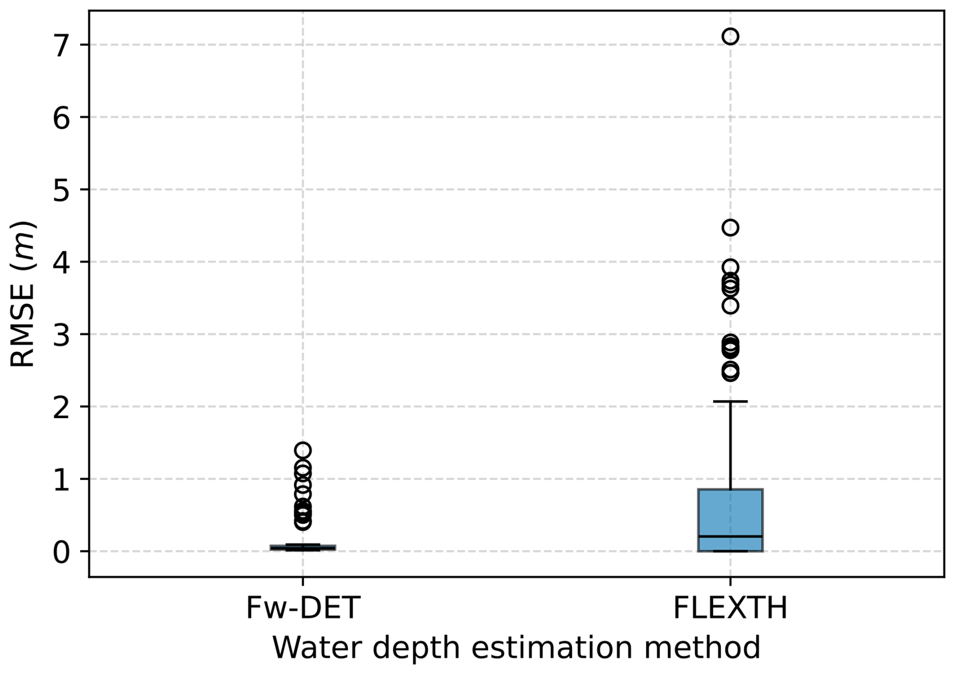
Figure 20 Box plot analysis of the variability induced only by water depth estimation hyperparameters for the 2 February 2021 acquisition.

While Fw-DET showed minimal variability in RMSE due to its hyperparameters alone (except for some outliers beyond the interquartile range), the FLEXTH method displays a much larger interquartile range of RMSE values. In this study, the Fw-DET method demonstrates more consistent performance. In contrast, FLEXTH, while potentially more accurate in ideal cases, was more sensitive to hyperparameter choices and could produce larger errors depending on the configuration used in each test case.

6 Discussion

This study evaluated the influence of preprocessing, flood mapping, and water depth estimation methods using SAR imagery for hydraulic applications. Our results highlighted that each stage, from speckle filtering to method choices and hyperparameter tuning, introduced variability that can propagate through to the final outputs.

6.1 Limitations of the evaluation process

The first limitation of the study was the unavailability of ground truth data for flood maps and water depth fields in the study area. As an alternative, hydrodynamic simulations were used as a reference for evaluating performance. These simulations introduce their uncertainties due to discretization, modeled physical processes, or roughness parameterization. Then, some of the observed discrepancies between estimated and reference values may stem from errors in the hydrodynamic model rather than from the methods used to extract the information in this study. Although the availability of a reliable reference would enhance validation, the primary goal of this study was to quantify the variability introduced by preprocessing, method choices, and hyperparameter settings. However, to select the most accurate method, it is essential to use test cases where independent ground truth is available. For instance, Landuyt et al. (2018) used Copernicus Emergency Management Service flood maps extracted from SAR or optical data, and Li et al. (2018) used labeled optical images (in cloud-free conditions) to validate SAR-based flood maps. In future works, we could also consider the uncertainty of the outputs of the physics-based model in the model evaluation process, based on GLUE analysis as proposed in Huang and Merwade (2024).

In this study, hyperparameter tuning was not uniformly exhaustive across all methods. For instance, traditional flood mapping methods were evaluated across a range of hyperparameter settings, while supervised classification methods were applied using fixed configurations. This may limit their performance and underestimate their potential under optimal settings or hide their variability due to hidden hyperparameters. Although we analyzed a range of key hyperparameters, additional influential parameters may be embedded within the methods themselves. Nevertheless, we believe that the primary sources of uncertainty were adequately captured by the parameters examined in this study. Future work could expand the range of hyperparameters considered and apply uncertainty quantification techniques, such as sensitivity analysis, to quantify the influence of each parameter on the outcomes by using more exhaustive Design of Experiments. For instance, Ghosh et al. (2024) showed the impact of the choice of model architecture when using convolutional neural networks for flood mapping and that the importance of polarization band combinations in the performance of supervised classification. For the change detection algorithms, the only hyperparameter was the choice of thresholding method (KI or Otsu) while Tupas et al. (2023) showed that Bayes change detection could be more robust to hyperparameter changes.

The flood mapping methods applied in this methodology rely on a single polarization, although most SAR satellites, such as Sentinel-1, provide multiple polarization channels. In this work, the VV polarization was not exploited, and the flood mapping approaches could potentially benefit from the additional information it provides. Nevertheless, for the considered test case, the inclusion of an additional polarization (VV polarization) in the training procedure of supervised classification did not lead to significant improvements in the evaluation metrics (variation of the flooded area below 0.1 km²).

The intercomparison of the methods and their hyperparameterization was tested exclusively on flooded scenes. In practice, practitioners may also require methods that perform reliably under dry conditions. For the flood mapping step, supervised classification and active contour methods can be applied in both flooded and dry scenarios. In contrast, the remaining approaches rely on the automatic detection of thresholds from image histograms and fail to discriminate between flooded and dry pixels when the histogram is not bimodal which is the case under dry conditions. Consequently, supervised classification methods or alternative implementations of change detection approaches (Tupas et al., 2023) may be preferred, as the change detection method used in this work depends on the automatic identification of a threshold in bimodal histograms, a condition that is generally only met during flood events.

6.2 Hydraulic analysis and implications for flood monitoring

The results of this study highlight that the quality of flood maps and water depths estimates is highly sensitive to preprocessing choices, method selection, and hyperparameter tuning. If the uncertainty in the generated output is high, the derived products may propagate errors into the hydrodynamic models, leading to inaccurate parameter estimation. For instance, Fig. 9 highlights that most configurations led to an underestimation of the flooded area compared to simulations. In this work, a fixed parameterization was used, but in a calibration context, if the variability due to flood map processing is more important than the changes in simulated flood maps due to the roughness parameter, the calibration could be complicated. Ideally, the variability in the observations should be smaller than the variability in the simulations.

To analyze the variability of the simulated flood maps due to the model parameterization, we evaluated the hydrodynamic model for the 2021 flood event using three Design of Experiments (DoE) consisting of 2000 parameter samples under different Strickler roughness configurations described in Table 2.

Figure 21 compares the 95 % variability range in simulated flooded area for each DoE with the flooded areas obtained using various flood mapping configurations for the 2 February 2021, SAR acquisition. The variability in the simulated flooded area is limited for DoE 1 and was lower than the variability across SAR-derived flood mapping methods. This complicates calibration because uncertainty from SAR processing dominates over that from model parameters. For the second DoE, the larger variation in floodplain roughness resulted in a wider range of flooded areas (approximately 5 km²), which is comparable to the variability observed for each SAR method, except for the active contour method. For DoE 3, there is a large spread in simulated flood extents, which is similar to the spread between methods (for instance, between the change detection median and the CNN median). For this study, only the CNN flood mapping method intersected with the simulation for DoE 1 and the median for the thresholding, change detection and Random Forest methods are close to the lower range of DoE 3. While this comparison on the flooded area can help to calibrate the model and identify subdomains where the Strickler should be adjusted, the uncertainty of the extracted flood maps should be taken into account during a calibration process. For instance, we mentioned that the CNN tends to overestimate the flooded surface even if it seems closer to the simulations. Thus, it is necessary to have a relevant evaluation methodology to compare the simulations and observations given their uncertainties as discussed in Travert et al. (2025) and Landwehr et al. (2024). Using data assimilation, both of the uncertainty of the generated flood maps and the uncertain numerical model (due to the uncertain Strickler parameters) can be taken into account to optimize the parameter values. Furthermore, when calibrating flood numerical models, given the uncertainty of generated flood maps, the modeler should be cautious and consider an ensemble of flood maps or use the most unfavorable test case to estimate conservative Strickler values and avoid non-conservative simulations.

Water depth estimation methods produced water depth fields with RMSE errors of around 2 m (for the median). These errors are too significant to be ignored in the calibration of this study area. Then, the calibration should be spatially constrained to areas where water depth estimates are more reliable, such as zones with low topographic gradient.

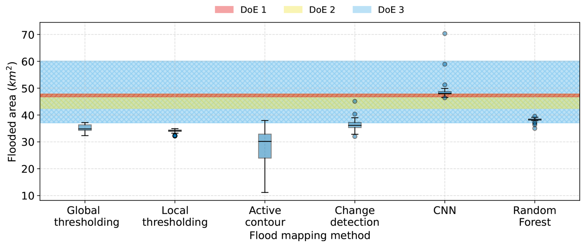
Figure 21 Comparison of flooded area variability from hydraulic simulations using three Design of Experiment (DoE 1–3) against SAR-based flood maps. The colored surface for the three DoE indicates the 95 % confidence interval of simulated flooded areas.

7 Conclusions

By systematically evaluating the impact of preprocessing, flood mapping, and water depth estimation methods and their hyperparameters, this study aimed to inform best practices for generating flood maps and water depth fields from SAR imagery. It contributes to improving the reliability of SAR-based hydraulic applications by underscoring the importance of assessing the influence of speckle filtering and hyperparameter choices. Rather than relying on a single fixed configuration, the findings highlight the need for a comprehensive evaluation of processing options. These options can significantly impact the extracted flooded areas or water depths, ultimately influencing the calibration and validation of hydraulic models. The choice of speckle filtering method was shown to significantly influence the statistics of SAR images, with deep learning methods such as the SAR2SAR approach outperforming the traditional approaches. For flood mapping, supervised classification methods demonstrated the highest median accuracy, F1-score and closest flooded area, but overestimating the flood extent size and leading to important errors in the water depth estimation step. Unsupervised methods such as thresholding and change detection offered reliable results with minimal tuning, making them suitable for rapid deployment. We highlighted the role of the speckle filter method choice and its hyperparameter on the flooded area estimates, with variations in flooded area estimates. The hyperparameters of the flood mapping methods were also influential on the generated flood maps, especially for active contour models. Three methods for estimating water depth fields were compared, showing that the accuracy of water depth estimation is strongly influenced by both the quality of the input flood maps and the parameterization of the methods. In this study, and for the tested hyperparameters, FLEXTH and Fw-DET exhibited similar performance. For studying the water depth on cross-sections, the cross-section analysis results in similar estimates but with a high variability depending on the cross-sections or input flood maps.

In future flood studies using SAR imagery for hydraulic applications, the role of preprocessing, method choices, and hyperparameter tuning should be evaluated to account for the errors due to the processing pipeline. We studied only SAR images, but similar methodologies to evaluate the impact of method choices and hyperparameters could be applied to optical satellite images.

Appendix A: Complements on flood mapping methods

A1 Global thresholding

For computing the threshold distinguishing flooded from dry pixels, two methods are used:

• Otsu's method selects the threshold that maximizes the between-class variance, which separates the histogram of pixel intensities into two distinct classes. The between-class variance is defined as:

  $$\begin{array}{}\text{(A1)}& {\mathit{\sigma }}_{\mathrm{B}}^{\mathrm{2}}={\mathit{\omega }}_{\mathrm{f}}{\mathit{\omega }}_{\mathrm{b}}({\mathit{\mu }}_{\mathrm{f}}-{\mathit{\mu }}_{\mathrm{b}}{)}^{\mathrm{2}},\end{array}$$

  where μ_f and μ_b are the mean intensities of the background and foreground classes, respectively. ω_f and ω_b are the foreground and background class fractions, respectively.

• The Kittler and Illingworth (KI) method also considers a mixture of two Gaussian distributions. The optimal threshold separates both classes by minimizing a cost function that quantifies the overlap between the distributions and is calculated as follows:

  $$\begin{array}{}\text{(A2)}& \begin{array}{rl}J& =\mathrm{1}+\mathrm{2}\left({\mathit{\omega }}_{\mathrm{f}}\log \left({\mathit{\sigma }}_{\mathrm{f}}\right)+{\mathit{\omega }}_{\mathrm{b}}\log \left({\mathit{\sigma }}_{\mathrm{b}}\right)\right)\\ & -\mathrm{2}\left({\mathit{\omega }}_{\mathrm{f}}\log \left({\mathit{\omega }}_{\mathrm{f}}\right)+{\mathit{\omega }}_{\mathrm{b}}\log \left({\mathit{\omega }}_{\mathrm{b}}\right)\right),\end{array}\end{array}$$

  where σ_f and σ_b are the standard deviations of the foreground and background classes, respectively.

A2 Local thresholding

The three conditions to keep a tile in the local thresholding approach are evaluated with three quantitative coefficients:

• Ashman's D coefficient (Ashman et al., 1994), which quantifies the separation between two Gaussian distributions, and is defined as:

  $$\begin{array}{}\text{(A3)}& \mathrm{AD}={\displaystyle \frac{|{\mathit{\mu }}_{\mathrm{f}}-{\mathit{\mu }}_{\mathrm{b}}|}{\sqrt{\mathrm{0.5}({\mathit{\sigma }}_{\mathrm{f}}^{\mathrm{2}}+{\mathit{\sigma }}_{\mathrm{b}}^{\mathrm{2}})}}}.\end{array}$$

• Bhattacharyya Coefficient (Bhattacharyya, 1943), which quantifies the amount of overlap between two distributions, and is computed as:

  $$\begin{array}{}\text{(A4)}& \mathrm{BC}=\sum _k\sqrt{\mathrm{hist}\left(y_k\right)}\sqrt{{\mathrm{hist}}_{\mathrm{f}}\left(y_k\right)},\end{array}$$

  where y is the pixel values in the tiles, “hist” is the histogram of the distribution, and hist_f is the fitted histogram with two Gaussian curves, and k is the bins of the two discrete histograms.

• The surface ratio is defined as the ratio of the area (measured in number of pixels) covered by the smaller population (e.g., dry or flooded pixels) to that of the larger population.