A workflow to identify and monitor slow-moving landslides through spaceborne optical feature tracking

Identifying and monitoring unstable slopes is essential for preventing both direct and cascading disasters triggered by landslides. To this end, we introduce TerraTrack, an open-source, cloud-based, end-to-end optical feature tracking tool for slow-moving landslide detection and monitoring. The tool is designed to run on the Sentinel-2 Level 1 harmonized collection. Users can define the area of interest, automatically download and pre-process Sentinel-2 data, and compute displacements using different feature tracking techniques. Outputs include a landslide binary mask, velocity maps and time series. The tool can operate entirely in the Google Colaboratory cloud environment. Hence, it removes the need for local computational resources and for a fast internet connection, avoids software conflicts, and is accessible even to those with limited experience in Python programming. We validated the workflow using displacement estimates obtained independently with other feature-tracking tools and expert landslide delineation across the Slumgullion, Chaos Canyon, and Tessina–Lamosano sites. We believe the tool is a valuable resource for the multi-hazard and landslide communities, complementing InSAR for monitoring surface motion in space and time. The tool can estimate motion shortly after the satellite imagery is acquired, making it an asset for early warning systems that rely on time of failure estimates (i.e., inverse velocity) or predictive modelling of future motion, within the limitations of satellite-based approaches. Lastly, its capacity to identify unstable slopes can guide targeted investigations into landslide dynamics, enhance situational awareness and support risk mitigation at scale.

1 Introduction

Landslides are among the most destructive geohazards, often interacting with other hazards in ways that amplify their impacts and trigger cascading events (Froude and Petley, 2018). For instance, earthquakes can trigger widespread landsliding (Tanya et al., 2022), while landslides themselves can generate secondary hazards such as floods – either by failing into lakes and causing glacial lake outburst floods (GLOFs) (Sattar et al., 2025) or by damming rivers (Fan et al., 2018).

While many of these hazards occur rapidly and with little warning, some landslides evolve more gradually, providing a window for observation and intervention. Slow-moving landslides can undergo progressive deformation over extended periods and may accelerate before catastrophic failure (Hungr et al., 2014; Lacroix et al., 2020), though failure does not always occur. Unlike rapid landslides, this behavior offers a critical opportunity for early detection and forecasting (Intrieri et al., 2012; Lacroix et al., 2018, 2020). Retrospective studies have demonstrated that such precursory motion can serve as a warning signal (Tordesillas et al., 2024) and can also be used to forecast failure time (Intrieri et al., 2012).

Given the widespread nature of landslide-prone terrain and the potential for extensive impacts, it is crucial to detect and monitor unstable slopes over large areas. Traditional ground-based mapping methods face challenges because of the vast areas involved, limited accessibility, and risks in surveying these regions (Guzzetti et al., 2012). Remote sensing, particularly spaceborne approaches, offers a viable alternative, as satellite and aerial imagery can be interpreted to map landslides efficiently (Santangelo et al., 2015; Mondini et al., 2019). Recently, the combination of AI and spaceborne images showed potential in quickly mapping failed landslides over large areas (Amatya et al., 2021; Meena et al., 2023; Fang et al., 2024). Such approaches are mostly applied to rapid (failed) landslides (Novellino et al., 2024), and they leverage change-detection based features (Nava et al., 2026), and/or the spectral contrast between the landslide scar and the surroundings (often vegetated areas) (Prakash et al., 2021). However, slow-moving landslides often exhibit only subtle surface changes, making them difficult to detect in standard satellite imagery. Consequently, researchers frequently use methods such as expert interpretation, stereophotogrammetry, or lidar to identify the morphological features of slow-moving landslides, although these approaches do not always indicate whether the landslide is active. In contrast, techniques like interferometric synthetic aperture radar (InSAR) (Monserrat et al., 2014; Crosetto et al., 2016), topographic change detection (Giordan et al., 2013), and feature tracking (FT) (Gance et al., 2014; Van Wyk de Vries and Wickert, 2021) can identify unstable landslide areas (slopes that are currently moving). Among these, Interferometric Synthetic Aperture Radar (InSAR) and its variants – such as Differential InSAR, Persistent Scatterer InSAR (Ferretti et al., 1999; Crosetto et al., 2016), and the Small BAseline Subset (SBAS) (Berardino et al., 2002) technique – are the most widely used. These methods can measure millimeter- to centimetre-scale displacements in the satellite's line of sight (LOS). When both ascending and descending satellite orbits are available for a given area, it is possible to derive a 2D displacement field, for example vertical and east-west (EW) displacement components (Tofani et al., 2013). However, InSAR has limitations: it performs poorly in densely vegetated areas, struggles to detect north-south (NS) motion due to the radar's side-looking geometry, and is less effective for rapid ground movements. Another approach is digital elevation model (DEM) differencing, which can capture vertical displacements by comparing terrain elevation changes over time (Prokešová et al., 2014). While useful for large, rapid changes, its accuracy depends on the resolution and quality of the DEMs, making it less effective for detecting subtle and horizontal movements.

The gaps left by InSAR and DEM differencing can be addressed with FT, which is particularly effective for measuring larger displacements and remains robust in environments where InSAR struggles – such as heavily vegetated regions or rapidly moving terrain (Van Wyk de Vries et al., 2024). Unlike InSAR, FT allows for the computation of displacements vectors in the entire 2D plane of satellite view, making it a valuable complement to vertical displacements offered by radar-derived ground motion estimates.

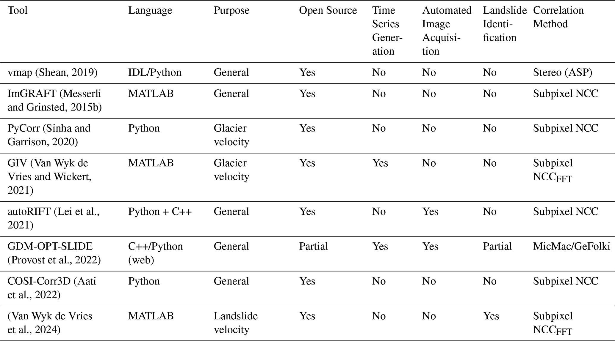
Few open-source FT routines can both detect landslide displacements and produce ground motion time series. These are essential for understanding landslide dynamics over longer periods. General-purpose FT software is often tailored to phenomena such as earthquakes or glaciers, which involve faster and more extensive movements than landslides (Messerli and Grinsted, 2015a; Van Wyk de Vries and Wickert, 2021). Because these tools rely on different data-processing strategies, they are less suited to capturing the smaller, slower movements characteristic of landslides. Table 1 shows a list of FT tools that can be easily used on spaceborne data. This highlights the need for a modular, open-source tool specifically designed for landslide detection and time series generation, one that supports automated image acquisition, cloud-based processing, and is implemented in an open programming language. Furthermore, since local expertise can greatly enhance the interpretation of feature-tracking results, we aim to make this approach accessible to non-experts in remote sensing.

Here, we propose TerraTrack, an open-source optical FT workflow specifically designed for slow-moving landslide detection and monitoring. TerraTrack uses the Google Earth Engine API to process Sentinel-2 Level-1 data and to automatically download it and computes displacements using various FT techniques. Its output use, landslide binary masks, velocity maps, and displacement time series, are generated entirely in the Google Colaboratory environment. The modular design of TerraTrack allows for flexibility and scalability, making it possible to adapt the framework to different geographical contexts and data sources. TerraTrack fills a critical gap in existing FT tools, offering a comprehensive solution that not only can detect unstable slopes but also can monitor their dynamics.

(Shean, 2019)(Messerli and Grinsted, 2015b)(Sinha and Garrison, 2020)(Van Wyk de Vries and Wickert, 2021)(Lei et al., 2021)(Provost et al., 2022)(Aati et al., 2022)(Van Wyk de Vries et al., 2024)

Table 1 Non-exhaustive list of codes and toolboxes that may be used for feature tracking on spaceborne data, their characteristics, and associated references. “General” indicates a general-purpose feature tracking framework. “Partial” refers to tools that are only partly open source or accessible through registration (e.g., via the Geohazards Exploitation Platform or ForM@Ter services) rather than through full public code release.

2 Case Studies

We select Slumgullion, Chaos Canyon, and Tessina-Lamosano areas to validate our workflow against independent displacement estimates and showcase its applications. Slumgullion, a well-documented case, serves as a benchmark to compare our FT with existing estimates. Chaos Canyon shows how FT time series could have signaled instability before failure. Tessina and Lamosano contrast two slow-moving landslides with different velocities, highlighting the limitations and complementarity of FT and InSAR for monitoring.

2.1 Slumgullion

The Slumgullion landslide is a ≈4 km-long, ≈0.5 km-wide earthflow situated in the San Juan Mountains, Colorado, USA (Parise and Guzzi, 1992; Coe et al., 2003). The actively moving section, estimated to have a volume of 2.0×10 m³ (Parise and Guzzi, 1992), is embedded within a larger, inactive flow that extends approximately 2 km downslope, ultimately damming Lake San Cristobal, Colorado's largest natural lake. This landslide serves as an excellent test case for our workflow as it has been extensively studied over the past decades, providing a wealth of remote sensing and ground-based measurements for validation. Also, it is situated in a complex mountainous terrain with variable vegetation cover and a lake, creating conditions where feature-tracking algorithms may encounter challenges (Van Wyk de Vries et al., 2024). Lastly, the active landslide is nested within a larger inactive flow, making it difficult to delineate their boundary without velocity measurements.

2.2 Tessina-Lamosano

The Tessina and Lamosano landslides, located in the Veneto region of northeastern Italy, provide an ideal setting to assess the performance of FT across different landslide velocity regimes. The Tessina landslide is a relatively fast-moving earthflow, while the Lamosano landslide is a very slow-moving rotational landslide in the same area. The Lamosano landslide has an estimated volume of 4.5×10⁶ m³ (Teza et al., 2008) and moves at velocities ranging from 2.8 to 10 cm yr⁻¹. It is currently shifting WSW, causing structural damage to buildings. The Tessina landslide is a complex, active earthflow, approximately 3 km long and up to 500 m wide. Since its initiation in 1960, it has undergone multiple reactivations, particularly in 1992 and 1995, largely due to heavy rainfall and snowmelt (Cola et al., 2016). It consists of a rotational slide source area, a channelized section where materials become fluidized, and an accumulation zone extending toward the villages of Funes and Lamosano. Velocity measurements for Tessina have varied over time, with movement typically in the range of several meters per year, reaching exceptionally up to 8 m yr⁻¹ (Cola et al., 2016).

2.3 Chaos Canyon

The Chaos Canyon landslide, located in Rocky Mountain National Park, Colorado, USA, collapsed on 28 June 2022. Prior to its failure, the landslide exhibited movement rates of approximately 5 m yr⁻¹ from 2017 to 2019, accelerating to 17 m yr⁻¹ in 2019. The collapse occurred during peak snowmelt, following a decade of higher-than-average positive degree day sums, suggesting a possible link to climatic factors. The landslide involved an estimated volume of $(\mathrm{1.26}\pm \mathrm{0.15})\times {\mathrm{10}}^{\mathrm{6}}{\mathrm{m}}^{\mathrm{3}}$ of material deposited at the slide toe (Morriss et al., 2023) Additionally, the alpine environment provides an excellent opportunity to test the workflow's ability to suppress noise caused by permanent snow patches, seasonal snow variability, water bodies, and the complex terrain of high-altitude, erosion-prone landscapes. Evaluating the workflow under these conditions helps assess its robustness in differentiating actual ground displacement from false signals in high-relief, dynamic alpine environments.

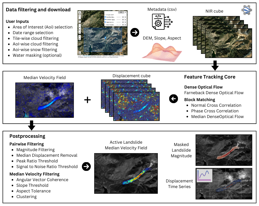
Figure 1 Workflow showing the main steps in our slow-moving landslide identification and monitoring workflow. Basemap sources: Esri 2025 | Powered by Esri (First line) and Copernicus Sentinel-2 imagery 2025 (Second and third line).

3 Methodology

We propose a workflow (Fig. 1) that identifies the location, extent, and dynamics of active slow-moving landslides without relying on any prior location information. Our workflow retrieves and processes Sentinel-2 Level 1C data cubes, along with DEM, slope, and aspect data for a user-defined Area of Interest (AoI). At its core, TerraTrack supports multiple matching algorithms – including Fast Fourier Transform-based Normalized Cross-Correlation (NCC_FFT), Phase Cross-Correlation (PCC), and dense optical flow – for measuring ground displacements. Automated identification algorithms then apply customizable spatiotemporal filters to isolate displacement patterns indicative of the presence of a slow-moving landslide. The tool ouputs an active landslide mask, a median displacement rate map, and displacement time series in a format compatible with existing QGIS plugins, i.e., InSAR Explorer (Haghshenas Haghighi, 2025).

3.1 Data Acquisition and Preprocessing

We use the Google Earth Engine Application Programming Interface to automatically acquire and preprocess Sentinel-2 Harmonised imagery (https://developers.google.com/earth-engine/datasets/catalog/COPERNICUS_S2_HARMONIZED?hl=it, last access: 12 May 2025). This corresponds to the Sentinel-2 Level-1C Products. We chose it as it is available up to 2015, unlike the Surface Reflectance (Level-2A) available from the 2017. In this framework, all parameters are fully customizable, enabling users to tailor data selection to their specific AoI and analytical requirements. The temporal extent is defined by a user-specified start and end year (e.g., 2016–2025), with an additional optional seasonal window (e.g., 1 January to 30 December) to filter out unfavorable periods. Optionally, users can set an initial and final collection date, useful for back analysis in studies where the failure time is known or some specific periods are of interest. At the tile level, a maximum cloud cover threshold (e.g., 50 %) is enforced, while further refinement is achieved by discarding images that exceed customizable thresholds for intra-AoI cloud (e.g., 5 %) and snow (e.g., 5 %) coverage. Users may also opt to mask water bodies. Specifically, cloud percentage is computed using the QA60 band (QA60 >0), while snow is identified by a Normalised Differenced Snow Index (NDSI) greater than 0.4, and water with a Normalised Difference Water Index (NDWI) >0. Moreover, the maximum number of images per year can be adjusted to balance temporal resolution with processing efficiency. The AoI is interactively defined by the user drawing a polygon on an interactive satellite base map provided by the geemap interface, with the resulting digitized feature collection serving as the basis for subsequent analyses. The outputs include a filtered Sentinel-2 Near Infrared (Band 8) data cube at 10 m (as Van Wyk de Vries and Wickert, 2021 show this achieves the best results), complementary morphological rasters derived from the NASA SRTM Digital Elevation 30 m (https://developers.google.com/earth-engine/datasets/catalog/USGS_SRTMGL1_003?hl=it, last access: 12 May 2025), and a .csv metadata file including Image ID, acquisition timestamp date, tile level cloud cover, orbit number, and tile ID. Slope and aspect are computed from the DEM using the functions ee.Terrain.slope(dem) and ee.Terrain.aspect(dem), respectively.

Before performing feature tracking, users can choose either to apply an orientation filter to enhance local spectral contrasts (Van Wyk de Vries and Wickert, 2021) and standardize the resulting orientation images for cross-correlation or to normalize images to 8-bit pixel values for optical flow.

3.2 Feature Tracking Algorithms

Broadly, FT algorithms fall into two categories: optical flow and chip matching. Optical flow methods comprise several families, including differential, matching-based, and energy-minimization approaches (Barron et al., 1994; Beauchemin and Barron, 1995). In contrast, chip matching partitions the image into smaller chips and aligns these chips between images to measure the displacement of each chip, providing localized motion estimates (Philip et al., 2014). In our workflow, we incorporate both approaches. We implement dense optical flow using the Farneback method (Farnebäck, 2003) a differential optical flow method (available for single pairs) and offer chip matching options that include NCC_FFT, PCC, and the median of Farneback optical flow within each chip.

We generate all possible image pairs using a multiple-pairwise image correlation approach (Stumpf et al., 2017). Customizable minimum and maximum temporal baselines are incorporated to adapt to the expected target velocity. Increasing the maximum baseline enhances sensitivity to more subtle ground motion but also increases the likelihood of temporal decorrelation. Conversely, reducing the minimum baseline improves the ability to detect faster surface displacements. Offset is estimated using chip-wise cross-correlation algorithms, applying a single-pass approach with customizable window size and overlap. In our implementation, a sliding window extracts chips from both images. Subsequently, one of three matching functions, NCC_FFT, PCC, or dense optical flow, is applied to estimate displacement.

NCC_FFT accelerates the computation of normalized cross-correlation by leveraging the convolution theorem to evaluate the correlation surface in the frequency domain. Prior to matching, both the reference and target chips are converted to zero mean to reduce sensitivity to absolute brightness differences. Given a reference chip R(x,y) and a target chip T(x,y), we define the mean-subtracted chips as $R^{\prime }(x,y)=R(x,y)-\stackrel{\mathrm{‾}}{R}$ and $T^{\prime }(x,y)=T(x,y)-\stackrel{\mathrm{‾}}{T}$.

The normalized cross-correlation surface is then computed in the frequency domain as

$$\begin{array}{}\text{(1)}& {\mathrm{NCC}}_{\text{FFT}}(u,v)={\mathcal{F}}^{-\mathrm{1}}\left({\displaystyle \frac{\mathcal{F}\left(R^{\prime }\right)\cdot \mathcal{F}(T^{\prime }{)}^{*}}{\sqrt{\sum \left|\mathcal{F}\right(R^{\prime }){|}^{\mathrm{2}}\sum |\mathcal{F}\left(T^{\prime }\right){|}^{\mathrm{2}}}+\mathit{ϵ}}}\right)\end{array}$$

where ℱ denotes the Fourier transform, ^* indicates complex conjugation, and ϵ is a small constant added for numerical stability. The inverse Fourier transform ℱ⁻¹ yields a correlation surface in the spatial domain, where the location of the maximum value corresponds to the best-matching displacement (u,v) between the two chips.

PCC is a frequency-domain technique that estimates the translational offset between two image patches by analyzing the phase shift in their Fourier transforms. Unlike NCC, which uses both amplitude and phase, PCC relies exclusively on the phase information. PCC is computed as:

$$\begin{array}{}\text{(2)}& \mathrm{PCC}(u,v)={\mathcal{F}}^{-\mathrm{1}}\left({\displaystyle \frac{\mathcal{F}\left(R\right)}{\left|\mathcal{F}\right(R\left)\right|}}\cdot {\displaystyle \frac{\mathcal{F}(T{)}^{*}}{\left|\mathcal{F}\right(T\left)\right|}}\right)\end{array}$$

The result of this expression is a correlation surface in the spatial domain, where the location of the global peak corresponds to the pixel-level displacement (u,v) between the two chips. PCC is particularly effective for subpixel registration when the images differ primarily by a rigid translation and are free from significant intensity or contrast differences. We implement both a custom version of PCC and an alternative provided by the skimage.registration module (Guizar-Sicairos et al., 2008). Both NCC_FFT and PCC support several adjustable subpixel refinement strategies, including centroid, parabolic, Gaussian, intensity peak gradient (IPG), and the offset-smoothing variants (os3, os5, os7). All subpixel refinement methods are detailed in the Supplement. In addition to displacement estimates, this method provides quality metrics such as the peak-to-peak ratio (PKR) and the signal-to-noise ratio (SNR). The PKR quantifies the sharpness of the correlation peak as the ratio between the highest and second-highest correlation values, providing a measure of match uniqueness (e.g., Van Wyk de Vries and Wickert, 2021). The SNR represents the ratio between the main correlation peak and the mean background correlation, indicating the confidence of the displacement estimate (Kanade and Okutomi, 2002). Median Dense Optical Flow per Chip applies the Farneback algorithm (Farnebäck, 2003) to compute dense optical flow within each chip. The local flow vectors are then aggregated by taking the median, for mitigating noise in cases where the flow field is irregular. After processing all chips, the displacement vectors are aggregated to form a gridded displacement field.

3.3 Active Slow-Moving Landslide Area Identification

Identifying active slow-moving landslides involves several post-processing steps aimed to refine displacement measurements and enhance the reliability of detected motion. We apply filtering at two stages: first, each pair is filtered independently. Second, we filter the aggregated median displacement map. Overall, these filters aim to suppress noise, and remove spurious detections.

For each image pair, we constrain the magnitude range to exclude unreliable measurements, setting an upper bound at the chip size (in pixels) minus one pixel (maximum measurable displacement). To mitigate misalignment, we remove the median displacement of the entire AoI (assuming non landslide area > landslide area in the AoI). Additionally, we add adjustable PKR and SNR thresholds. Several additional filtering steps are available in the workflow, which can be enabled or disabled depending on the specific requirements of the analysis. Zero mask filtering can be used to exclude areas that are likely to generate undesired noise (e.g., water or glaciers). Deviation filtering identifies and excludes displacement vectors that fall outside a defined threshold when compared to the local median displacement magnitude within a 5×5 window. A 1D median filter can be applied to smooth valid displacement vectors, reducing noise but potentially blurring sharp, localized motion gradients. Angular coherence filtering (Eq. 3) retains displacement vectors whose directions closely align with a locally smoothed angular field (6×6 pixels).

The resulting median displacement map undergoes additional refinement steps to isolate coherent motion patterns. Magnitude thresholding is applied first to retain only targeted ground movements: here, a user-defined threshold, based on expected landslide motion rates or the 95th percentile of the magnitude distribution within the area, is used to exclude small displacements. Similarly to the pairwise filters above, we apply angular coherence filtering. Vectors deviating from locally coherent directions (typically more than 30°) are removed via the following equation:

$$\begin{array}{}\text{(3)}& \begin{array}{rl}\text{Angular deviation}& =\left|\right(\text{median angle}-\text{smoothed angle}\\ & +\mathit{\pi })\mathrm{mod}\mathrm{2}\mathit{\pi }-\mathit{\pi }|\end{array}\end{array}$$

while vector coherence – which considers both displacement magnitude and direction – has been used in other studies to assess motion consistency (Stumpf et al., 2017), we choose to rely solely on angular coherence. Slow-moving landslides often exhibit sharp spatial variations in velocity due to changes in terrain, material properties, or localized accelerations. By filtering only based on direction, we avoid incorrectly discarding active landslide areas where displacement magnitudes fluctuate. Displacement vectors are limited to areas with slopes steeper than a user-defined threshold, excluding flat regions. Aspect-based filtering further removes vectors that deviate beyond a set angular tolerance from the downslope direction:

$$\begin{array}{}\text{(4)}& \begin{array}{rl}\text{Angular difference}& =min\left(\right|\text{vector angle}-\text{aspect}|,\mathrm{360}\mathit{°}\\ & -|\text{vector angle}-\text{aspect}|)\end{array}\end{array}$$

To remove isolated outliers and retain spatially coherent groups indicative of genuine landslide activity, we apply density-based clustering (DBSCAN). The algorithm preserves regions where at least n displacement points fall within a N-pixel radius, while excluding scattered, low-density points. Finally, morphological post-processing enhances spatial coherence in the landslide mask. We apply a sequence of operations: bridging to connect isolated pixels, to ensure local consistency, filling to remove holes within detected landslide areas, and thinning to refine boundaries (Van Wyk de Vries et al., 2024). The resulting masked median velocity map can optionally be corrected for slope angle effects, under the assumption of a vertical satellite viewing angle.

The final output is a landslide displacement mask that delineates zones of persistent, slow-moving landslides.

3.4 Time-Series Generation

Time-series generation of surface displacement is useful for landslide dynamics investigations and warning systems (Nava et al., 2023). To accommodate different research needs, our workflow offers multiple approaches for constructing time series, allowing users to select the most appropriate method based on their specific objectives. The output time series is saved in a format compatible with the “InSAR Explorer” Plugin in QGIS (Haghshenas Haghighi, 2025).

The first approach assigns the velocity value to the midpoint between the two acquisition dates. After users can compute the yearly or monthly median of the velocity values to create a more aggregated and smoothed time series.

A second method involves converting the displacement measured in each image pair to a velocity, which is then distributed uniformly across the days spanned by the pair. These daily values are subsequently aggregated by taking the median of all values falling within a specified time window, defined in months and adjustable by the user. While this approach allows for the generation of denser time series, it introduces uncertainty due to the relatively long temporal baselines between image pairs – often exceeding one year. As a result, care must be taken when interpreting short-term trends, as they may reflect interpolated averages rather than precise, time-localized displacements.

The third approach employs a sparse least-squares framework to recover a velocity time series from discrete displacement observations. We solve the optimization problem ${min}_{\mathbf{x}}{∥W(A\mathbf{x}-\mathbf{b})∥}_{\mathrm{2}}^{\mathrm{2}}$, where each observation i contributes a displacement $b_i=v_i\cdot \frac{(t_{\mathrm{2},i}-t_{\mathrm{1},i}{)}_{\text{days}}}{\mathrm{365.25}}$, with v_i the annualized velocity between times t_1,i and t_2,i (Paige and Saunders, 1982). The design matrix $A\in {\mathbb{R}}^{N\times M}$ satisfies $A_{i,j}=\mathrm{1}$ if day $T_j\in [t_{\mathrm{1},i},t_{\mathrm{2},i}]$, and 0 otherwise. The diagonal matrix $W\in {\mathbb{R}}^{N\times N}$ optionally applies weights based on observation quality (based on SNR or PKR). The solution x∈ℝ^M yields velocities at the chosen temporal resolution and is resampled into coarser bins (e.g., monthly) using the median. This formulation is mathematically analogous to SBAS-style linear inversion approaches (e.g., expressing observations as integrals over unknown velocities) (Berardino et al., 2002).

A key consideration is that our workflow operates with temporal baselines usually above 1 year, meaning that the time intervals between velocity measurements can be quite large. Despite this, we can still generate monthly time series by interpolating or aggregating available displacement estimates. However, this approach introduces some uncertainty, particularly when assigning velocities to the midpoint date – as the difference between the mid-date and end-date reference can be up to 2.5 years. Specifically, the resulting timeseries will be heavily smoothed. This must be taken into account when interpreting temporal trends, as displacement estimates may not always correspond to precise monthly-scale motion but rather reflect an averaged velocity over longer observation periods.

Alternatively, the final displacement cubes can be converted in a TICOI-compatible format (Temporal Inversion using Combination of Observations and Interpolation) (Charrier et al., 2025), that allows for more advanced time-series reconstruction methods.

4 Results

To assess the performance of the subpixel refinement methods under controlled conditions, we applied known subpixel shifts (0.1-pixel steps) to a Sentinel-2 image (Supplement). This benchmark allowed us to evaluate the accuracy (Normalized Median Absolute Deviation – NMAD) and bias of each method independently of terrain complexity or image noise from real cases. Among the tested methods, Center of Mass, Parabolic, os3, and os5 showed the best agreement with the applied shifts, capturing the imposed displacements with moderate bias. The remaining methods performed poorly and were excluded from further analysis. Based on these results, we used these four best-performing methods in the Slumgullion test case.

Figure 2 Median displacement magnitude maks and map of the Slumgullion landslide computed by PCC with subbixel refinement by (a) os3, (b) os5, (c) parabolic, and (d) center of mass. Extents from Hu et al. (2020). Basemap provider: Esri 2025 | Powered by Esri.

4.1 Slumgullion

Here we demonstrate how displacement results at the Slumgullion landslide vary depending on the different FT subpixel refinement approaches supported by TerraTrack and we compare them with previous estimates.

The Sentinel-2 NIR image cube consists of 43 acquisitions spanning from 14 September 2016 to 7 October 2024, resulting in a total of 564 image pairs with temporal baselines ranging between 1 and 5 years.

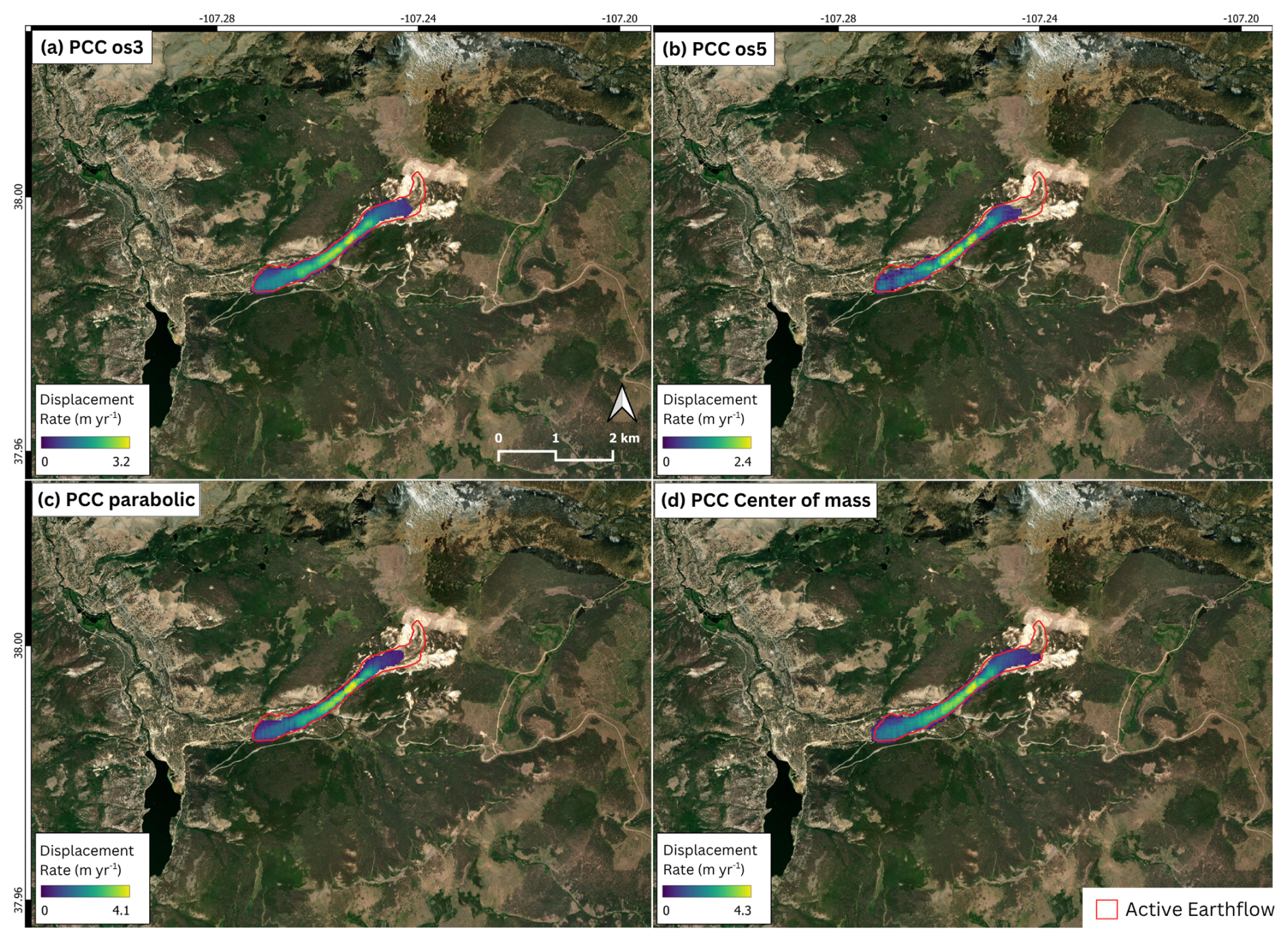
For all methods, we use a chip size of 16 pixels with 80 % overlap. From each displacement map, we remove values with magnitudes exceeding the chip size minus one pixel (i.e., the maximum measurable displacement). We subtract the median displacement of the entire area of interest (AoI) from each map and apply a peak-to-correlation ratio (PKR) threshold of 1.3 and a signal-to-noise ratio (SNR) threshold of 3. For the median displacement map (Fig. 2), we apply additional refinement using a 0.5 m yr⁻¹ velocity threshold, a 30° angular dispersion filter, a minimum slope of 5°, and a 45° aspect tolerance. Finally, we retain only groups of at least 20 vectors located within a 20-pixel radius.

We evaluate four subpixel refinement methods, selected based on the benchmark analysis provided in the Supplement. These are assessed in terms of displacement magnitude, detected landslide area, computational time, and the presence of overpredictions or noisy motion fields. All four methods successfully delineate the main body of the Slumgullion landslide. The center-of-mass refinement yields the highest maximum displacement, reaching approximately 4.3 m yr⁻¹ in the central-eastern sector. The same area is also detected by os3, os5, and parabolic refinements, with slightly lower peak values of 3.2, 2.4, and 4.1 m yr⁻¹, respectively.

A detailed benchmark comparison of NCC_FFT and PCC, each combined with various subpixel refinement strategies, is available in the Supplement. For the specific configuration applied at Slumgullion, the per-block runtime (in s) for PCC was $\mathrm{3.43}\times {\mathrm{10}}^{-\mathrm{5}}$ for parabolic refinement, $\mathrm{5.66}\times {\mathrm{10}}^{-\mathrm{5}}$ for center of mass, $\mathrm{8.70}\times {\mathrm{10}}^{-\mathrm{5}}$ for os3, and $\mathrm{9.97}\times {\mathrm{10}}^{-\mathrm{5}}$ for os5. To contextualize this, processing 564 image pairs of size 673 × 975 pixels using PCC with center-of-mass refinement required 2950.74 s (i.e. 49 min).

All four configurations (center of mass, os3, os5, and parabolic) produce comparable landslide masks and closely match the active deformation area reported by Hu et al. (2020). Among these, center of mass and os3 refinements appear slightly more sensitive to low-magnitude displacements, extending the mapped deformation further upslope into the headscarp zone. This suggests greater responsiveness to subtle ground motion in these particular configurations. At the same time os3 and os5 yeld lower median velocities than center-of-mass and parabolic refinements. Lastly, the median field in os5 appears less smooth than the one produced by the other methods. None of the tested methods resulted in significant overpredictions or spurious displacement patterns in this case study.

In terms of maximum velocity (reference value $\approx \mathrm{4.4}\mathrm{m}{\mathrm{yr}}^{-\mathrm{1}}$ from Van Wyk de Vries et al., 2024), os5 underestimates ($\approx \mathrm{2.4}\mathrm{m}{\mathrm{yr}}^{-\mathrm{1}}$), os3 is slightly lower ($\approx \mathrm{3.2}\mathrm{m}{\mathrm{yr}}^{-\mathrm{1}}$), while Parabolic and Center of Mass are closer (≈4.1 and $\approx \mathrm{4.3}\mathrm{m}{\mathrm{yr}}^{-\mathrm{1}}$, respectively). We select os3 for the following cases because, despite the slightly lower magnitude at Slumgullion, os3 showed (i) the lowest NMAD_x and NMAD_y in the synthetic benchmark, (ii) the lowest bias, indicating more accurate and stable displacement estimates, and (iii) stable performance in all other landslides.

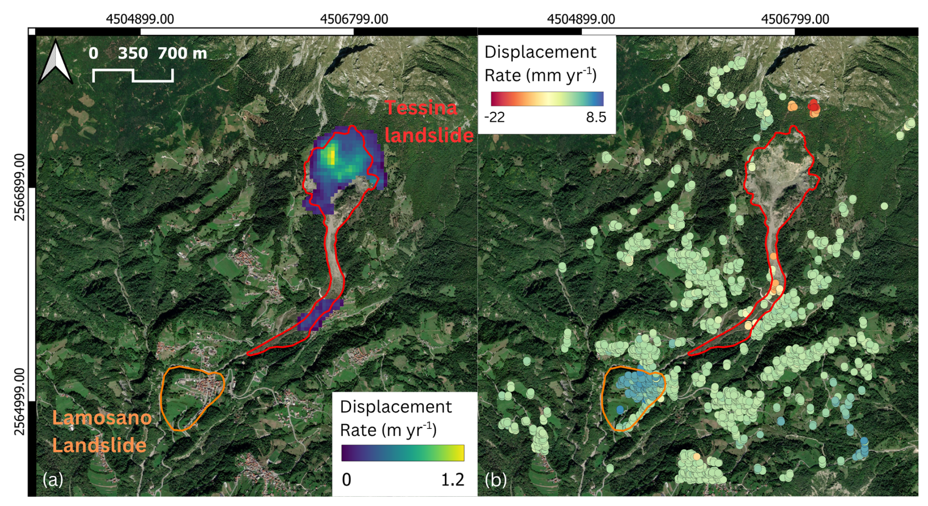
Figure 3 (a) Median displacement magnitude map of the Tessina landslide computed with PCC and os3 subpixel refinement and (b) InSAR velocity from EGMS L2a Ascending VV (Line of sight displacement). Landslide boundaries were manually digitized using recent high-resolution Google Earth imagery, based on geomorphological indicators such as scarps, tension cracks, and vegetation changes. The mapping was guided by the sector delineations reported in van Westen and Lulie Getahun (2003). As a result, the boundaries represent areas showing morphological evidence of past or potential instability, rather than confirmed actively moving zones. Basemap provider: Esri 2025 | Powered by Esri.

4.2 Tessina-Lamosano

Here we showcase the complementarity of TerraTrack and InSAR in identifying slow-moving landslides.

Here, the Sentinel-2 NIR cube is composed of 220 images, spanning from 4 July 2015 to 2 May 2025. These make a total of 14 511 pairs with temporal baselines between 1 and 5 years.

We use the PCC method, with a chip size of 16 pixels, overlap 80 %, and os3 subpixel refinement. For each displacement mask generated from an image pair, we remove magnitudes above chip size minus one pixel. We remove the median displacement of the entire AoI to each map, we apply a PKR threshold of 1.3 and a SNR threshold of 3. For the median displacement map (Fig. 3), we refine the results by using the 95th percentile of magnitude over the AoI as minimum threshold (≈0.2 m yr⁻¹), 30° angular dispersion filter, a minimum slope threshold of 5°, and a 45° aspect tolerance. Finally, we retain groups of at least 20 remaining points within a 20-pixel radius.

The EGMS InSAR Level-2a product, derived from ascending orbit data in VV polarization, clearly captures the Lamosano landslide. It appears as a distinct red cluster in the lower right portion of the scene, with LOS velocities ranging from approximately 1.5 to 2.6 mm yr⁻¹. However, this dataset provides no useful information in the Tessina landslide headscarp, where velocities are generally higher, vegetation cover is dense, and motion occurs predominantly in the NS direction – conditions under which InSAR typically performs poorly. In contrast, our FT workflow effectively identifies and measures motion within the Tessina landslide, including in heavily vegetated areas. Here, the method captures much faster velocities, with median displacement rates reaching up to 1.8 m yr⁻¹. The FT-derived displacements also allow us to resolve the NS component of motion, which is generally inaccessible to InSAR due to the satellite's side-looking geometry.

However, the Lamosano village area is not detected by FT, as the displacement there is below the method's sensitivity threshold on Sentinel-2 10 m resolution imagery. This highlights the complementary nature of FT and InSAR: when used together, they offer a more complete understanding of ground motion dynamics. InSAR is sensitive to vertical and east – west motion but blind to NS motion, whereas FT can resolve horizontal components including NS, but lacks sensitivity to very slow movements and vertical displacements.

Overall, it is important to note that neither method can capture all deformation, but combining them expands the detectable velocity range and improves overall understanding of landslide motion in complex, landslide-prone terrain.

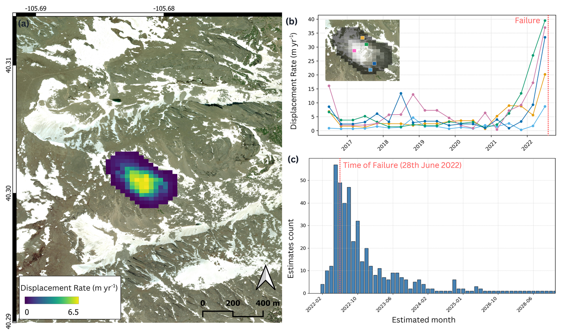
Figure 4 (a) Median displacement rate map of the Chaos Canyon landslide prior to failure. (b) Representative velocity time series derived from a least-squares inversion with a 1-month temporal resolution. Median values are then aggregated into 4-month intervals to construct smoothed time series. While values are assigned to the center of each 4-month bin, this does not imply that displacement occurred precisely at that time. This plot illustrates temporal variations in displacement rates across the landslide body. Time series from the western sector are generally noisier due to the presence of a semipermanent snow patch. (c) Distribution of estimated failure times derived via the inverse velocity method (Carlà et al., 2017); linear fits were applied to the last 3–5 observations from each FT time series. Basemap provider: Esri 2025 | Powered by Esri.

4.3 Chaos Canyon

This case shows TerraTrack as a support for estimating the time of failure of landslides.

Here, the Sentinel-2 NIR cube is composed of 100 images, spanning from 26 June 2016 to 20 June 2022 (failure occurs on the 28 June 2022). These make a total of 3014 pairs with temporal baselines between 1 and 5 years.

We use the PCC method, with a chip size of 16 pixels, overlap 80 %, and os3 subpixel refinement. For each displacement mask generated from an image pair, we constrain the magnitude range from 0 to chip size minus one pixel (maximum measurable displacement). We remove the median displacement of the entire AoI to each map, we apply a PKR threshold of 1.3 and a SNR threshold of 3. For the median displacement map (Fig. 4a), we refine the results by using the 95th percentile of magnitude over the AoI as minimum threshold (≈0.21 m yr⁻¹), 30° angular dispersion filter, a minimum slope threshold of 5°, and a 30° aspect tolerance. Finally, we retain groups of at least 20 remaining points within a 20-pixel radius. Time series (Fig. 4b–c) are generated using the least-squares inversion approach with a 4 months observations frequency. Most of the time series within the landslide body show an accelerating trend.

We apply the inverse velocity method (Carlà et al., 2017) to estimate the timing of failure for this landslide. We compute the inverse of velocity for each time series within the detected active landslide body, ensuring an objective and spatially distributed analysis. For each point, we fit a linear trend to the last 3 to 5 observations and extract the projected failure date. The distribution of these predicted failure times is shown in Fig. 4c. The mode of the distribution aligns with May 2022, the month before the landslide failure, with a high concentration of estimates also falling within the preceding and following two months.

5 Discussion

We validate and demonstrate the versatility of TerraTrack, showcasing its applications across a range of tasks – from identifying active landslide areas to monitoring their dynamics and estimating time of failure. TerraTrack is designed to be both intuitive and computationally efficient, with fully reproducible and well documented outputs. It marks a methodological step forward compared to existing tools in several important respects. Unlike previous approaches (Van Wyk de Vries and Wickert, 2021; Lei et al., 2021; Aati et al., 2022; Van Wyk de Vries et al., 2024), TerraTrack integrates automated image acquisition with advanced selection criteria to ensure optimal input quality for feature tracking. Provost et al. (2022) includes automated image acquisition, although the tool is not fully open-source. A further methodological difference is that MPIC-OPT relies on the GeFolki dense optical-flow – based co-registration algorithm (Charrier et al., 2020), whereas TerraTrack uses chip-based NCC_FFT/PCC matching with subpixel refinement.

A further advancement lies in its ability to identify the location and extent of slow-moving landslides using freely available Sentinel-2 imagery – unlike most previous studies that rely on airphotos or commercial high-resolution satellite data (e.g., Stumpf et al., 2017). While Van Wyk de Vries et al. (2024) also applies FT to detect landslides using Sentinel-2, their implementation lacks key capabilities such as automated image acquisition, time-series generation, and inverse velocity analysis.

Our workflow shares many of the known strengths and limitations of optical feature tracking approaches, such as those described in Van Wyk de Vries et al. (2024). As with any FT-based method, performance is constrained by surface decorrelation, persistent snow, and the need for coherent downslope motion. Very slow or highly intermittent landslides may not be captured, and false positives can occur in areas with correlated noise or unrelated surface displacements (e.g., glaciers, infrastructure motion, or coseismic effects). These challenges emphasize the importance of integrating FT with other data sources, such as InSAR or ground-based observations, and interpreting outputs with care. In addition, the use of an anisotropic filter mitigates most radiometric inconsistencies caused by shadows, although deep or variable shadows can still lead to local decorrelation. Dense vegetation and persistent or seasonally variable snow cover may reduce correlation quality in optical feature tracking, as changes in canopy structure or snow redistribution between acquisitions can introduce decorrelation noise. In addition, while TerraTrack can be executed in Google Colab for accessibility, large-area analyses may be limited by runtime and memory constraints, although the workflow can also be run locally or in alternative cloud environments with greater computational resources.

Although TerraTrack was primarily designed for slow-moving landslides, the feature-tracking framework itself is general. TerraTrack can be applied to glaciers using standard optical feature-tracking workflows. It can also be used to measure coseismic surface displacements: we implemented a dedicated option that constructs image pairs across a user-defined time window, allowing displacement to be computed specifically over the period when rapid motion occurred (e.g., pre- and post-earthquake imagery).

In addition, TerraTrack integrates multiple FT methods within a single environment, giving users flexibility to adapt workflows to different terrain conditions, processes, and displacement regimes. The performance comparison highlights key trade-offs between speed, sensitivity, and noise. PCC is as reliable as NCC_FFT in subpixel estimation while slightly faster (see Supplement). PCC combined with parabolic or center-of-mass refinement provides the fastest results, while os3 is slower but more robust to noise. Despite these differences, all methods delineate the main Slumgullion landslide body with broadly consistent spatial patterns. PCC with center-of-mass and os3 also capture smaller displacements in the headscarp area, suggesting higher sensitivity to low-magnitude motion. Overall, PCC offers the best balance between speed and accuracy, making it the most practical choice for large-scale or time-sensitive analyses. As for subpixel estimation, parabolic and center-of-mass methods offer faster performance but exhibit modest bias and noise. In contrast, offset-smoothing approaches (os3 and os5) yield more robust and accurate subpixel estimates, particularly in low-SNR conditions, though at a higher computational cost. Among these, os3 provides the best compromise between precision and efficiency. Subpixel measurements are inherently subject to bias and uncertainty, which can affect absolute motion magnitudes. However, these limitations do not impact the identification of stable versus unstable slope areas, and relative spatial patterns remain consistent and reliable. Overall, we recommend using PCC combined with parabolic refinement for fast processing, and os3 for intrinsically noisy environments, such as high mountain areas, noting that motion magnitudes there may be slightly underestimated.

We highlight the complementarity between FT and InSAR for ground motion analysis. Each method offers strengths that address the limitations of the other, FT can capture large, non-vertical displacements, also in vegetated areas while InSAR is sensitive to millimetre-scale motion, particularly in the vertical and east–west directions. Together, they enable a more complete picture of slope instabilities, particularly in complex terrains or in cases where landslides display heterogeneous behavior across space or time. This synergy is essential for improving both detection and interpretation in areas where relying on a single method would leave gaps. We also demonstrate that the time series derived from TerraTrack are useful for tracking landslide dynamics and can also be leveraged for estimating the timing of failure. It is worth noting that not every acceleration leading to failure will be captured. This is due to the coarse temporal resolution of the derived time series and the increased noise typically present at the beginning and end of the series, where image pairs are based fewer acquisitions, with respect to the center of the monitoring window. In the Chaos Canyon case, a back-analysis using inverse velocity methods yielded failure time estimates closely aligned with the actual event, suggesting potential for operational use in landslide warning systems.

The transition from retrospective validation to real-time forecasting requires further investigation. Key areas for future research include evaluating how predictive performance is affected by temporal resolution, noise levels, and the specific characteristics of the landslide. Future work will also focus on improving subpixel accuracy and better quantifying associated uncertainties. Beyond individual case studies, future work will focus on scaling the methodology for application at regional and national levels, enabling systematic detection and monitoring of slow-moving landslides across broad areas. The long-term vision is to integrate TerraTrack with large-scale InSAR datasets, creating a complementary system for operational landslide monitoring and early warning. While the framework is designed for scalability, site-specific knowledge remains critical for interpreting results, validating detections, and understanding local geomorphological context. By lowering technical barriers, we hope TerraTrack will empower a wide range of landslide researchers to apply these techniques within their own study areas.

6 Conclusions

We present TerraTrack, a workflow for spaceborne optical feature tracking, developed specifically for detecting and monitoring slow-moving landslides. The main innovations of TerraTrack are:

• End-to-end automation of optical feature tracking, from data acquisition to time-series output, designed to be accessible to non-experts through open-source tools and minimal user input.

• Quality-based image pair selection together with automated landslide delineation and time series generation, enabling direct extraction of spatial and temporal motion patterns.

• Retrospective failure-time estimation using freely available, medium-resolution Sentinel-2 imagery.

Through a series of case studies and benchmarks, we show that TerraTrack performs reliably across different landslide types and displacement behaviors. TerraTrack offers a practical and scalable tool for landslide research and hazard identification, monitoring and early warning.