Considering rainfall events from a neighborhood improves local flood frequency analysis

Many aspects of flood risk management require flood frequency analysis (FFA) which is, however, often limited by short observational records – especially for flash floods in small basins. In order to address this issue, we propose to extend the underlying data by local counterfactual scenarios. To that end, heavy precipitation events (HPEs) from nearby, hydrologically similar catchments are used to simulate flood peaks which are then included in the FFA for the catchment of interest. In order to demonstrate the added value of this approach, we used 23 years of radar-based precipitation and a hydrological model, fitted the Generalized Extreme Value (GEV) distribution to three different datasets – observed peaks, counterfactual peaks, and their combination –, and evaluated the resulting three GEV fits by means of the quantile skill score (QSS). For a sample of more than 13 000 German headwater catchments, we could show that local counterfactuals improved quantile estimation, with the level of improvement increasing with return period. The improvement declines when the radius of the transposition domain is extended beyond 30 km. Overall, our results provide a tangible perspective to enhance traditional FFA, producing narrower confidence intervals and more robust estimates for design floods and risk assessments.

1 Introduction

Flood frequency analysis (FFA) addresses the probability of floods of a given magnitude and their expected recurrence. It provides the statistical basis for defining extreme events and is, since decades, fundamental for various aspects of flood risk management (Klemes, 1993; Merz and Blöschl, 2008), such as the design of hydraulic infrastructure, landscape planning, flood insurance and many more.

Typically, extremes are extracted from observations (of, e.g. discharge or precipitation accumulated over specific durations) via the block maxima or peak-over-threshold method, and a probability distribution is fitted (Gumbel, 1958), most commonly the Generalized Extreme Value (GEV) or Generalized Pareto (GP) distribution. This allows extrapolation of the tail beyond observed records (Cooley, 2012) and an estimation of occurrence probabilities (return periods) for unobserved events.

However, extreme floods occur rarely (by definition), resulting in limited sample sizes for FFA. Short observational records can increase the sampling error and thus the uncertainty of distribution fitting. Consequently, estimates of occurrence probability are often highly uncertain, which can lead to a severe misrepresentation of risk. This problem is amplified in the case of flash floods: these floods are characterized by a rapid onset and carry high sediment and debris loads, which makes them a highly destructive natural hazard (Barredo, 2007; Llasat et al., 2010; Petrucci et al., 2019; CRED/UCLouvain, 2023). The corresponding rainfall events are typically brief and intense and occur at small spatial scales. They only trigger a flash flood in case they coincide with basins that are able to convert rainfall into runoff, and rapidly propagate that runoff towards the outlet. These processes are governed by topography, geomorphology, soils, and land use. Furthermore, flash-flood-prone basins are generally small to medium sized (<1000 km²). The local scarcity of extreme floods and the limited availability of corresponding streamflow records challenge conventional FFA for flash-flood risk management.

Several approaches have been proposed to address data scarcity and the limitations of FFA. Their central idea is to augment the data basis, either by incorporating information from hydrologically similar sites or by forcing hydrological models with hypothetical heavy precipitation events (HPEs). Following we will give a brief overview over existing concepts.

• Regionalization: Data from hydrologically similar catchments are incorporated into the estimation of distribution parameters to enhance the robustness of extreme value analysis (EVA) (e.g. Gaume et al., 2010; Guse et al., 2010; Nguyen et al., 2014; Halbert et al., 2016).

• Probable maximum precipitation (PMP): rainfall events from a “meteorological homogeneous” transposition domain are included in the analysis to increase the robustness (Fuller, 1914; District and Morgan, 1916) and to estimate the PMP (Hansen, 1987; WMO, 2009). Instead of exceedance probabilities this method only yields upper and lower bounds of precipitation. PMP can be used to estimate the upper bounds of a probable maximum flood (PMF), if used as forcing for a hydrological model. While PMP is widely applied in North America and Australia for designing high-risk infrastructure (e.g. dams and nuclear power plants), it is not used in Europe. However, in recent years various studies regarding flood risk management have proposed and investigated different concepts of storm transposition, referring to the idea as “spatial counterfactuals” (Montanari et al., 2024; Merz et al., 2024; Voit and Heistermann, 2024b; Vorogushyn et al., 2024; Thompson et al., 2025).

• Stochastic storm transposition: Building on the PMP/PMF concept, historical precipitation events (HPEs) from the transposition domain are sampled using a Poisson distribution and randomly assigned (uniform distribution) within the domain, potentially affecting the catchment of interest (CoI). For flood frequency analysis, the resulting runoff in the CoI is simulated (e.g. Wright et al., 2014). This approach allows for the calculation of occurrence probabilities. For a detailed description see Wright et al. (2017). Globally, stochastic storm transposition (SST) remains rarely applied in practice (Wright et al., 2020) but it will form the core of the US Federal Emergency Management Agency's “Future of Flood Risk Data” initiative, aimed at remapping the nation's floodplains (Abbasian et al., 2025).

• Random weather generators are statistical models that simulate sequences of weather variables, such as temperature and precipitation, by randomly generating data based on observed patterns. They can be used to generate very long time series of meteorological forcings for a hydrological model (e.g. Falter et al., 2015; Apel et al., 2016).

The central issue with these approaches is the plausibility of counterfactuals. Hazard assessments based on such methods are only meaningful if the counterfactuals are considered realistic. Due to the large variability in terminology with regard to the aforementioned concepts, we now clarify and define, for the sake of consistency, the following terms and acronyms for use throughout this paper:

• HPE: Heavy precipitation event. While sometimes termed “storms”, we adopt the more precise designation HPE.

• TD: Transposition domain; a region that is assumed to be meteorologically homogeneous (with respect to the features of heavy rainfall). The basic idea is, that an HPE observed within the TD, could have also happened at any other location within the TD.

• storm transposition: Spatial transposition (relocation) of an observed HPE within a TD.

• CoI: Catchment of interest, the catchment that is the subject of a FFA.

• NC: Neighboring catchment. A catchment in proximity to the CoI, typically within a TD.

• counterfactual: A hypothetical realization of an event under alternative conditions, e.g. an HPE occurring at a different location.

• factual peak. Flood peak observed in the CoI or modelled with observed rainfall.

• counterfactual peak: Flood peak simulated by a hydrological model forced with a transposed (counterfactual) HPE.

Previous studies have proposed different methods to define a TD from which HPEs are sampled. Fontaine and Potter (1989) described it as a region where “significant storms are uniformly distributed in space,” while Zhou et al. (2019) suggested using cloud-to-ground lightning analyses. However, the outcome of these methods also depends on the length of the observed data. Instead of defining a TD based on a complex analysis, Voit and Heistermann (2024a) introduced the concept of “local counterfactuals”: they selected HPEs that had caused high runoff peaks in basins from a close (i.e. “local”) neighborhood around the CoI (more specifically, a 20 km radius), transposed these events to the CoI and used it to force a rainfall-runoff model that would than return the counterfactual flood peak. The approach was based on the assumption that if an HPE were sampled from a local neighborhood, it would be more representative for HPEs that are “typical” for the CoI. Even with this local TD, local counterfactuals produced flood peaks comparable to a 200 year return level flood. By using the runoff reaction of nearby catchments as a filter to sample hydrologically meaningful HPEs for transposition, no previous detection and compilation of HPEs is required with this method.

But how can counterfactuals be incorporated into FFA? For numerous application contexts, return periods and design levels remain essential for stakeholders. SST provides one way to statistically assess the occurrence of hypothetical flood scenarios, but it requires both the definition of the TD and the selection of the most relevant rainfall duration for sampling events. The latter is not trivial, as the duration of extreme rainfall that generates the highest flood peak may vary between catchments and is often difficult to determine in advance. For this reason Voit and Heistermann (2024a) proposed a bottom-up approach by selecting the HPEs which caused high flood peaks nearby catchments, irrespective of rainfall duration.

In this study, we propose to extend the concept of local counterfactuals in order to formally integrate counterfactual flood peaks into flood frequency analysis (FFA). This is demonstrated in a case study on the basis of 23 years of radar-based precipitation records in Germany, in combination with a Germany-wide flash flood model as introduced by Voit and Heistermann (2024b): for each of 13 452 headwater catchments (<750 km²) in Germany, we fit three GEV distributions: (i) from the 23 annual flood peak maxima modelled in the basin of interest (our reference), (ii) from 230 counterfactual peaks derived by spatially transposing HPEs which caused 23 annual maximum peak discharge values in 10 hydrologically and topographically similar neighboring basins, and (iii) from the combined dataset. A 30 km radius neighborhood (transposition domain) can be still be considered as local and small, compared to the domain sizes in other studies (e.g. Voit and Heistermann, 2024b; Abbasian et al., 2025), and it is our prime filter to make sure we sample storms from an atmospheric environment that is governed by similar mechanisms as the CoI. Yet, sampling storms that caused annual maxima in similar catchments should ensure that the transposed rainfall has spatio-temporal characteristics that make them representative for the CoI (e.g. similar catchment size) and that could also occur over the CoI given potential orographic effects (e.g. similar catchment elevation). The number of 10 neighboring catchments was chosen mainly due to limited computational resources.

The quantile score (QS) (Bentzien and Friederichs, 2014) is then used to analyze whether counterfactual information improves the representation of extremes beyond the limited observational record. The QS can evaluate improvement for each quantile of interest. We repeat this procedure for four differently sized and shaped TDs and show how the design of the TD affects the results of the FFA. Finally, we discuss the return levels derived from the different GEV distributions and examine the corresponding confidence intervals.

2 Data

2.1 RADKLIM

We used the radar climatology product RADKLIM v2017.002 (2001–2023) to compute local counterfactuals and to drive continuous runoff modeling across Germany. RADKLIM is provided by Germany's national meteorological service (Deutscher Wetterdienst, DWD) and represents a reprocessed version (Lengfeld et al., 2019) of DWD's operational radar-based quantitative precipitation estimation product, RADOLAN (Winterrath et al., 2012). The dataset has a spatial resolution of 1 km×1 km, an hourly temporal resolution, and is openly available via the DWD open data server (Winterrath et al., 2018).

2.2 DEM

For catchment delineation and runoff analysis, we used the EU-DEM (European Commission, 2016), which has a 25 m resolution and combines SRTM (Shuttle Radar Topography Mission) and ASTER GDEM (Advanced Spaceborne Thermal Emission and Reflection Radiometer Global Digital Elevation Model).

2.3 Land use and soil data

Information on land cover was obtained from CORINE CLC5-2018 (BKG, 2018), which classifies high-resolution satellite imagery into 37 land cover classes for Germany following the European Environmental Agency (EEA) nomenclature. The classification considers objects with a minimum size of 5 ha and is updated every three years. Soil data were derived from the BUEK 200 national soil survey (scale 1:200 000; BGR, 2018), compiled from federal state surveys by the Federal Institute for Geosciences and Natural Resources (BGR) in cooperation with the National Geological Services (Staatliche Geologische Dienste). For each mapping unit, BUEK 200 provides areal fractions of dominant soil types along with detailed profile information, including texture, bulk density, and other key properties.

3 Methods

Much of the data and methodology for this study are detailed in Voit and Heistermann (2024b). Here, we briefly describe the hydrological model, further explain the flood frequency analysis, and the selection of local counterfactuals.

3.1 Modelling surface runoff

The hydrological model (Voit, 2024) was specifically tailored to simulate flash flood events in small- to medium-sized basins. A detailed model description is provided in Voit and Heistermann (2024b). During flash floods, surface runoff dominates (Marchi et al., 2010; Grimaldi et al., 2010), while evaporation and groundwater dynamics are negligible. Accordingly, the model comprises two modules. First, effective rainfall is estimated for each catchment and timestep (hourly) using the SCS-CN method (U.S. Department of Agriculture-Soil Conservation Service, 1972), which is widely applied in flash flood modeling (Gaume et al., 2004; Borga et al., 2007; Emmanuel et al., 2017). Since flash flood events predominantly occur during the summer months, we slightly adjusted the CN values for agricultural areas to account for the effects of summer crops (based on Seibert et al., 2020). A single CN value for each subbasin was then derived using an area-weighted average. Second, the geomorphological instantaneous unit hydrograph (GIUH), derived from the DEM, represents the concentration of quick runoff from effective rainfall. The flow velocities were computed with the method of Maidment (Maidment et al., 1996). This approach accounts for the increase in hydraulic radius with rising flow volumes, as described by Manning's equation, thereby capturing the downstream acceleration of flow without requiring the estimation of roughness coefficients for individual grid cells. In addition, it removes the need to distinguish between hillslope and channel grid cells within the catchment. The method assumes a velocity field that is invariant in both time and discharge, enabling the convolution of GIUHs to simulate the catchment response to the effective rainfall of an HPE. When two subcatchments converge, the hydrograph of the upstream basin is superimposed on that of the downstream basin with an appropriate time lag. This delay is defined by the travel time from the downstream basin's inlet to its outlet.

The model's lightweight design allows the computation of large numbers of counterfactual scenarios. As it does not account for channel hydraulics or engineered structures, the analysis is restricted to headwater catchments smaller than 750 km². Because of the lumped nature of the model it is crucial that the catchments are small enough to account for the spatial variability of rainfall. In our analysis, this corresponds to 13 452 sub-catchments with an mean area of 15.7 km² and a maximum headwater catchment size of 163 km².

3.2 Design of local counterfactuals

Local counterfactuals are HPEs drawn from a neighborhood (TD) of a given catchment of interest (CoI) – the catchment to which the counterfactual scenarios are applied, and transposed to the CoI. In this study, all aforementioned 13 452 headwater catchments smaller than 750 km² are individually treated as a CoI, meaning that the following procedure is applied to each of these catchments (see also Fig. 1 for illustration):

1. For each CoI, we identified the ten most similar catchments located entirely within a 30 km buffer around the CoI. We based similarity mostly on descriptors of topography, land use and soil which should (i) strongly govern the formation and concentration of surface runoff and (ii) ensure that potential orographic effects could occur both in the CoI and the NCs. Following descriptors were chosen:

   • Peak [m³ s⁻¹], time to peak [s] and standard deviation [m³ s⁻¹] of the unit hydrograph: The unit hydrograph is derived directly from the DEM, similar hydrographs imply, to a certain degree, similar topography.

   • Total catchment area including upstream basins.

   • Curve number (soil moisture class 2): The curve number represents soils and land use in our model. A similar curve number would lead to a similar runoff generation in our model.

   • Mean and standard elevation of the DEM and mean slope. With this descriptor we try to avoid sampling rainfall events from catchments which are e.g. situated at a substantially different elevation. If the CoI was e.g. close to a mountain range, rainfall events should not be sampled from this mountainous area, because they might not be representative for the rainfall events occuring in the CoI.

   • Unit Peak Discharge: The peak of the unit hydrograph divided by the catchment area is yet another descriptor of the hydrological character of the catchment.

   We used the KDTree-algorithm from the Python library “SciKit-Learn” and scaled all catchment descriptors with the “StandardScaler” from this library to ensure that none of this descriptors dominates the decision for similarity. However, we acknowledge that some descriptors are correlated.

2. For each of these NCs, we model the quick runoff from 2001 until 2023 (Fig. 1b). We then identify the annual maximum peak discharge for each of the 23 years (Fig. 1c).

3. From RADKLIM, we extract the data for the 23 HPEs which caused the annual maximum peaks in the NC (Fig. 1b) and transpose them from their original spatial position from the centroid of the NC to the centroid of the CoI, thereby creating spatial counterfactuals (Fig. 1d). We ensure that the CoI and all its upstream catchments will be completely covered by the HPE, by adding a 70 km buffer on each side of the RADKLIM subset (for better visualization we do not show the buffer in Fig. 1). To ensure a consistent soil moisture state we add a 14 d temporal buffer before the actual event. If the CoI consists of various subbasin, we additionally transpose the HPEs to the centroid of every upstream subbasin.

4. We model the surface runoff that these counterfactual HPEs would have caused in the CoI (Fig. 1e) and record the maximum counterfactual peak discharge values for each year. We repeat steps 3 and 4 for all NCs.

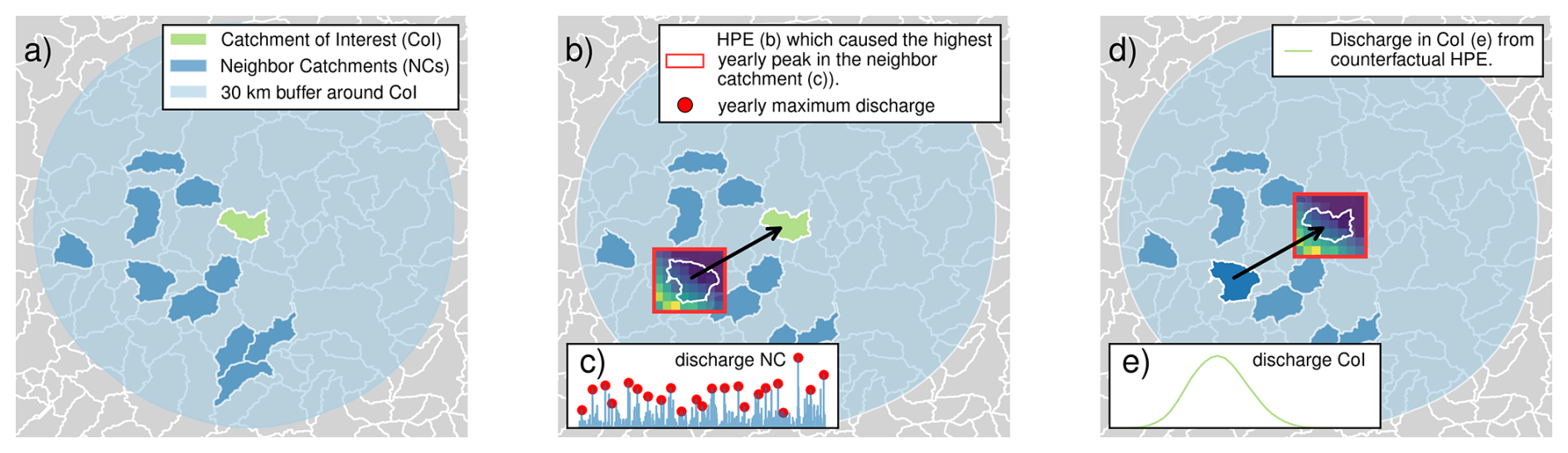
Figure 1 Development of local counterfactuals: (a) Catchment of Interest (CoI, green) and its 10 neighbor catchments (NCs, dark blue) in a 30 km neighborhood (light blue). (b) Selecting the HPE which caused the highest annual runoff peak (red dot, c) in the NC (red box). (d) Transposing the HPE from the NC to the CoI and modelling the resulting runoff (e). This procedure is repeated for each NC and steps (c–e) are repeated for each year.

We hypothesize that the representativeness of counterfactuals for the meteorological processes governing the CoI generally decreases with the distance between the corresponding NC and the CoI. To test this hypothesis, we compared four transposition domains (TDs): a 10 km buffer, a 30 km buffer, and two ring-shaped TDs with inner–outer radii of 30–60 and 60–90 km around the CoI, respectively.

3.3 GEV distribution

Under certain conditions, block maxima are GEV-distributed (Fisher and Tippett, 1928; Gnedenko, 1943). These conditions are met for precipitation (Coles, 2001) and discharge. The cumulative distribution function (CDF) of the GEV is defined

$$\begin{array}{}\text{(1)}& {\displaystyle }{\displaystyle }G\left(x\right)=\left\{\begin{array}{ll}\exp \mathit{\{}-{\left[\mathrm{1}+\mathit{\xi }\left(\frac{x-\mathit{\mu }}{\mathit{\sigma }}\right)\right]}^{-\mathrm{1}/\mathit{\xi }}\mathit{\}},& \mathit{\xi }\ne \mathrm{0}\\ \exp \mathit{\{}-\left({\exp }^{(z-\mathit{\mu })/\mathit{\sigma }}\right)\mathit{\}},& \mathit{\xi }=\mathrm{0},\end{array}\right.\end{array}$$

with location μ, scale σ and shape ξ.

From the GEV distribution, return levels can be obtained for return periods that are even longer than the length of record. However, this extrapolation is uncertain with limited sample size (Coles, 2001). Our suggestion is, hence, to increase the sample size with local counterfactuals. To fulfill the requirements of the Fisher–Tippet-Theorem, all block maxima have to be drawn from the same statistical distribution. We choose a very small area as TD and then select HPEs within this TD based on the streamflow response of neighboring catchments that are very similar regarding slope, elevation, land use and the unit hydrograph (see Sect. 3.2). Based on this similarity of catchments and the small TD, we regard this first requirement as fulfilled. Since the peaks of factual and counterfactual HPEs are determined with the same method, both can be pooled to fit a GEV, given all assumptions above. To fulfill the requirements of the Fisher–Tippet-Theorem, it is also paramount not to arbitrarily discard subsets of the data. More specifically, this mandates to include all annual maximum peak discharge values from an NC (instead of, e.g. just the highest one) to keep a consistent effective block size.

In FFA, special attention is given to the shape parameter ξ: a large shape parameter indicates a heavy tailed distribution where extreme events with high magnitude can occur. Especially when fitted to limited data points, the GEV distribution can produce implausible parameter estimates or “poor fits”. For this reason we disregard catchments where one of the previous GEV distributions has a shape <0 or shape $\ge \mathrm{0.5}.$ These thresholds are a compromise of values for ξ that are considered to be hydrologically plausible (Morrison and Smith, 2002; Merz et al., 2022). We used the Python package “scipy” (Virtanen et al., 2020) with a maximum likelihood estimator to fit the GEV distribution.

3.4 Quantile skill score

We utilize the quantile score (QS) (Bentzien and Friederichs, 2014) to quantify how a well a GEV distribution represents the quantiles of the series of annual block maxima from the CoI. First, the tilted check-function ρ_p(⋅) is used to compute a penalty for estimated quantiles in comparison to the data points z_n.

$$\begin{array}{}\text{(2)}& {\displaystyle }{\displaystyle }{\mathit{\rho }}_p\left(u\right)=\left\{\begin{array}{ll}pu,& u>\mathrm{0}\\ (p-\mathrm{1})u,& u\le \mathrm{0}\end{array}\right.\end{array}$$

With $u=z_n-q$. For high non-exceedance probabilities p (which corresponds to a return period $T=\frac{\mathrm{1}}{\mathrm{1}-p}$), it leads to a strong penalty for data points that are still higher than the modeled quantile (z_n>q).

The quantile score is then computed for each non-exceedance probability p:

$$\begin{array}{}\text{(3)}& {\displaystyle }{\displaystyle }\text{QS}(y,q;p)=\sum _i^n{\mathit{\rho }}_p(y_i-q)\end{array}$$

with p-quantile q (a return level corresponding to T), tilted check-function ρ_p(⋅) and block maximum y_i obtained from the n factual peaks in the CoI.

We estimate the parameters of three GEV distributions that are fitted on different subsets of data and refer to them as follows:

• GEV_CoI: fitted only to the factual peaks from the CoI.

• GEV_NCs: fitted only to the counterfactual peaks from the NCs.

• GEV_all: fitted to both factual peaks from the CoI and the counterfactual peaks from the NCs.

Essentially, GEV_NCs and GEV_all are the GEV variants that we introduce as competitors against the conventional GEV_CoI which is exclusively based on information obtained in the CoI. In order to verify the added value of the new GEV variants, GEV_CoI serves as a reference. For this purpose, we use the quantile skill score (QSS) which compares the QS of GEV_NCs and GEV_all (denoted QS_NCs and QS_all, respectively) to the QS of our reference GEV_CoI (QS_CoI) as follows:

$$\begin{array}{}\text{(4)}& {\displaystyle }{\displaystyle }{\text{QSS}}_i=\mathrm{1}-{\displaystyle \frac{{\text{QS}}_i}{{\text{QS}}_{\text{CoI}}}}\text{ with }i\in \mathit{\left\{}\text{NCs, all}\mathit{\right\}}\end{array}$$

The QSS can take values between minus infinity and 1. Positive values indicate that the competing GEV (GEV_NCs or GEV_all) is superior to the reference.

As the quantile score (Eq. 3) is always computed for a specific return period T (or non-exceedance probability p), the QSS itself is obtained for specific values of T, too (20, 50, 100, and 200 years in this study), similar to Fauer and Rust (2023, Fig. 4). Note that for very high return periods the QS might become unreliable, since only few or low observations are higher than the evaluated quantile. Then, the QS might just reward the model that predicts the lowest quantile.

The reference QS_CoI itself is obtained by means of a leave-one-out cross-validation: to that end, one year i is excluded from the CoI's series of factual annual maxima and the GEV_CoI is estimated from the remaining training years. From the fitted GEV_CoI,i, a return level (p-quantile) is calculated and a quantile score QS_CoI,i is determined from this return level and the annual maximum value for year i. This is repeated for all years in the CoI series. QS_CoI is then obtained as the average of all QS_CoI,i.

4 Results and Discussion

4.1 Verifying the added value of counterfactual peaks on GEV estimation

For each small-scale basin in Germany, we created local counterfactuals (Sect. 3.2) and used these counterfactual flood peaks to fit a GEV distribution for the CoI. To validate how well local counterfactuals are able to represent the quantiles in the data (the factual flood peaks in the CoI), we performed an out-of-sample-test by comparing the GEV_NCs with the GEV_CoI.

The inspection of the GEV parameters for each catchment reveals a large number of implausible shape parameters, especially for GEV_CoI, which is fitted to only 23 year-maxima. Because the number of data points increases by adding counterfactual peaks, the fits for GEV_NCs improve: about 29 % of the basins cannot be included in the analysis because the implausible fit of GEV_CoI whereas 5 % of the catchments have to be excluded because of an implausible fit of GEV_NCs (see Sect. 3.3). In total this leads to an exclusion of ≈ 33 % of the basins.

Figure 2 shows the results for all TDs and for four different return periods (20, 50, 100, and 200 years). Since negative values of the QSS are harder to interpret, we show only QSS≥0. We will discuss the differences between the different TDs in the following section. For now, we focus on the TD with a radius of 30 km. The main result is that the GEV_NCs – which has never seen any information from the CoI – clearly outperforms the GEV_CoI: across all return periods and transposition domains, the majority of catchments have positive QSS values. E.g., for the TD with a 30 km buffer, the percentage of catchments with positive QSS_NCs values (see intercept on the y axis) is 87 % for T=20 a, 78 % for T=50 a, 73 % for T=100 a, and 69 % for T=200 a. Evidently, GEV_NCs performs worse for the corresponding remainder to 100 %.

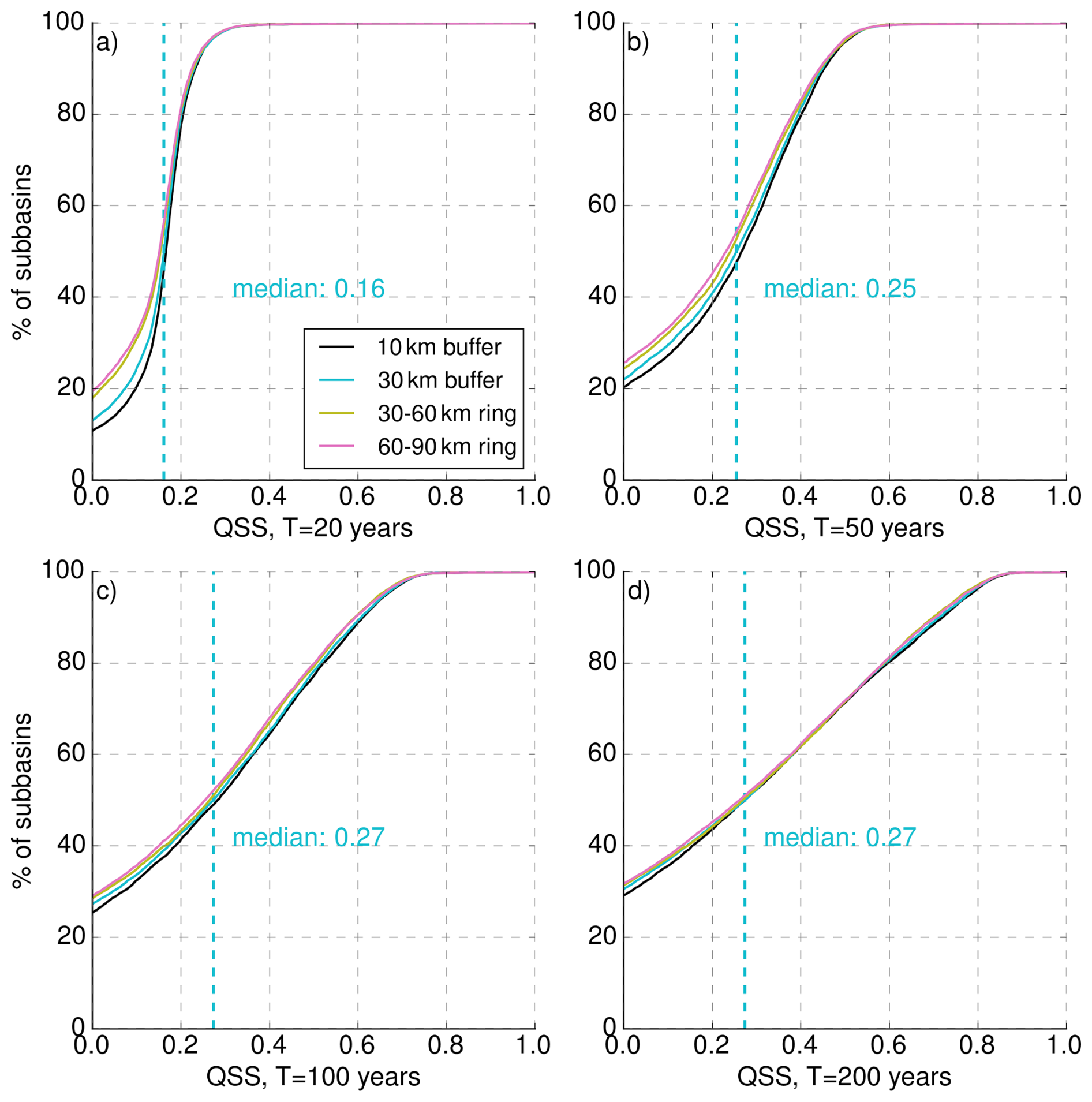
Figure 2 Cumulative distributions showing the quantile skill scores for GEV_NCs in reference to GEV_CoI, for all subbasins and for four different transposition domains (10 km buffer: black, 30 km buffer: blue, 30–60 km ring: yellow, 60–90 km ring: pink. Subplots (a–d) show different quantiles that relate to the (a) 20 year, (b) 50 year, (c) 100 year, and (d) 200 year flood. A quantile score >0 indicates the superiority of the GEV_NCs. The median QSS of the 30 km buffer is indicated with the vertical blue dashed line.

We would like to take a closer look at the differences between the return periods. Increasing return periods lead to a decreasing fraction of catchments with positive QSS_NCs values – obviously not desirable -, but also to a desirable increase of catchments with very high QSS values (for T=20 a, 0.2 % of the catchments have a QSS>0.5, while this fraction grows to 28 % for T=200 a). Altogether, the median QSS continuously grows from a value of 0.16 for T=20 a to a value of 0.27 for T=200 a, suggesting that the value added by using GEV_NCs increases with the return period. This is plausible, since return levels for low return periods can be estimated more robustly from short time series (for T=20 a, the estimation of a return level from an annual series of 23 years does not even imply extrapolation). The uncertainty increases the more we extrapolate beyond the length of the annual series. Especially for high return periods the benefit of an increased data basis is visible in these results.

These results serve as a proof of concept: for the majority of cases, we are able to better represent the quantiles in the data of the CoI by using a GEV distribution fitted exclusively to the counterfactual peaks (GEV_NCs). Besides the fact, that the counterfactual peaks represent the distribution of CoI peaks well, the GEV_NCs is also more robust because it is fitted to 230 values, instead of the 23 values used for GEV_CoI. The improvement is more pronounced for higher quantiles (or return periods). In practice the GEV would be fitted to both factual and counterfactual peaks together (GEV_all), which only marginally increases the robustness of the return level estimates. The QSS for GEV_all is shown in Fig. S1 in the Supplement.

4.2 Effect of different transposition domains

We calculated the QSS_NCs for four different TDs. This way, we want to investigate whether HPEs transposed from larger distances are less “typical” for the CoI and will therefore result in less representative GEV fits with lower values of QSS_NCs. This effect can be observed in Fig. 2. For each return period, the intercepts of the QSS distributions on the y axis are higher for the ring-shaped TDs (30–60 and 60–90 km) than the intercepts of the TDs with a 10- or 30 km buffer. This effect is less pronounced with increasing quantiles. The differences between the 10- and 30 km-buffers are very small. These results support the hypothesis that HPEs transposed over short distances are more representative for the HPEs occurring directly over the CoI. Nevertheless, the sampling process of the NCs can also have an impact on the results. Within the TD we sample ten catchments which are most similar to the CoI (Sect. 3.2). If the TD is very small, there are less basins to sample from so that the representativeness of the sampled HPEs for the CoI might suffer. Likewise it could also be possible that basins are less similar to each other with increasing distance. Due to the complex topography around every catchment, we think that there can be hardly a generalized solution for the “perfect” transposition domain. However, our results show, that there is, for most small-scale basins in Germany, no large difference whether the TD is a 10-, or 30 km buffer. Providing large computational resources this could be systematically investigated further by increasing the size of the TD step by step and evaluating the QSS.

4.3 Return levels

We would now like to demonstrate how the use of local counterfactuals affects return levels, in comparison to the conventional use of factual discharge peaks in the CoI. While GEV_NCs was used for verification in Sect. 4.1, we will now use GEV_all because there is no reason to entirely discard the data from the CoI for GEV fitting. For the 200 year return period, Fig. 3 shows the ratio between the return level obtained from GEV_all and from GEV_CoI (as a histogram over all analysed catchments). For all TDs, the median ratio is very close to one, so using local counterfactuals results in lower return levels for half of the basins and to higher return level for the other half. In our view, this is an important insight: in contrast to our intuitive expectation, the use of local counterfactuals for GEV fitting does not systematically increase the resulting return levels, but simply reduces the estimation error over all CoIs (based on the higher QSS and the narrower confidence intervals, see below). However, this improvement of the GEV estimation is still based on the inclusion of higher discharge maxima via counterfactuals. This is illustrated by the gray histograms in Fig. 3 which show, for each catchment, the ratio between the highest value in the annual maximum series of counterfactual and factual peaks and the highest value in the annual maximum series of just the factual peaks. The gray histograms clearly show that counterfactuals increase the maximum of the complete series of annual maxima, leading to more robust GEV fits. The medians for all TDs are between 1.43–1.6. It is important to note that the four TDs cover very different spatial extents: the 30–60 km-ring has an area of 14,137 km², while the 10 km buffer has a size of ∼466 km² (for a circular basin with an area of 15 km²). The larger the TD we sample HPEs from, the more options we have to find catchments which are very similar to the CoI. Thus, it is also more likely that we are sampling HPEs that matter regarding the formation of an extreme flood peak in the CoI. This absolute maximum peak could serve as reference for the probable maximum flood (PMF) and is automatically included in the results of the analysis. Yet, remember that sampling from such more distant and larger neighborhoods does not improve the GEV estimation, as was shown in Sect. 4.2.

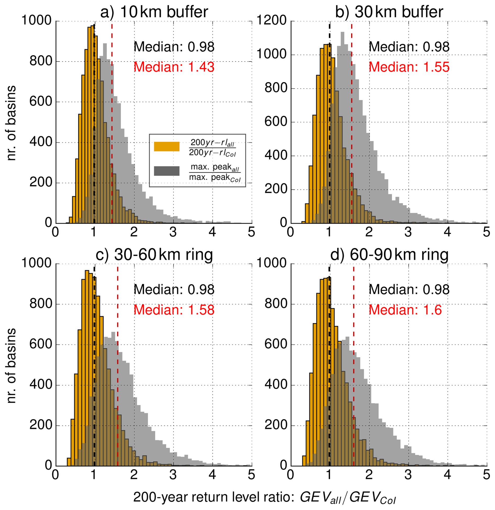
Figure 3 Histogram of the ratio between the 200 year return level from GEV_all and from GEV_CoI for four TDs. Gray histograms indicate the ratio of the highest peaks in the respective datasets used for fitting (see main text for further explanation). The median ratio of the return levels ratio is marked in black, and the median ratio of maximum peak discharge values in red.

The difference between the two medians shown in Fig. 3 may appear counterintuitive. However, two factors account for this observation. First, although the counterfactual dataset exhibits some higher peaks, these peaks occur jointly with the entire set of annual maxima from this NC (23 values for each NC). In many cases these high peaks have little impact on the GEV fit due to the amount of data points that are just “average” peaks. Figure 4 shows an example of this case. The sampling error with small sample sizes as the 23 annual maxima for the GEV_CoI can lead to very heavy tailed GEV fits, high return level estimates and very wide confidence intervals. Even though the data pool for GEV_all (253 values) contains more extreme peaks (max. CoI: 43.2 m³ s⁻¹, max. all: 87.3 m³ s⁻¹), the fit is still mainly influenced by the larger amount of moderate peaks and results in lower return level estimates.

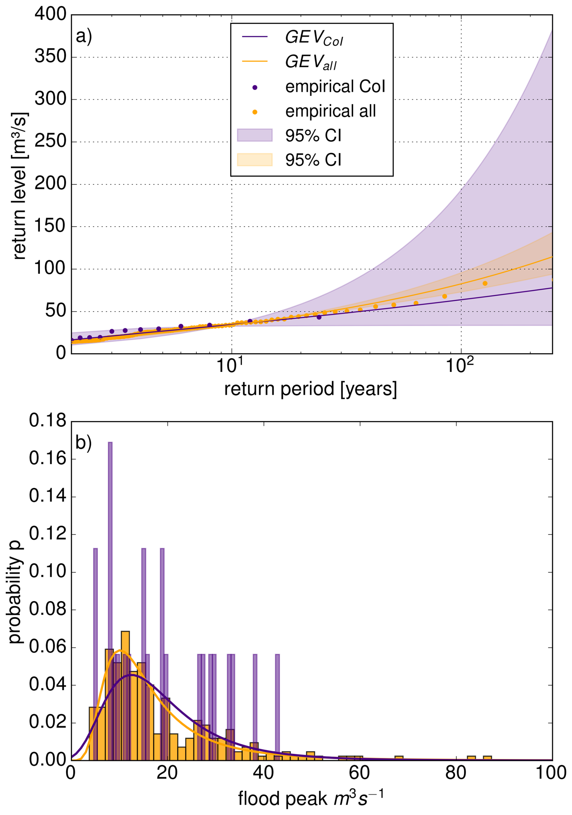
Figure 4 Comparison of two GEV_CoI and GEV_all for one exemplary basin. (a) Return levels estimated by GEV_all (orange) are lower than by GEV_CoI (purple). The shaded areas mark the 95 % confidence interval estimated with boot strapping (n=500). The empirical return periods were estimated with the Weibull plotting position and are indicated with the semi-transparent dots. (b) Density histogram of the annual maxima and fitted GEV distribution.

Secondly, local counterfactuals also induce spatial smoothing (which is desired): each catchment is a CoI once, but serves as neighbor for many other CoIs. As a result, nearby and hydrologically similar catchments often share almost identical sets of peaks. When a counterfactual peak increases the return level estimate for one CoI, the peaks from that CoI will also enter the NC data pool once their roles are reversed. In this case, the inclusion of the peak can reduce the return level estimate for the neighboring catchment.

The estimation of return levels beyond the observational period comes with large uncertainties in the case of GEV_CoI in the example in Fig. 4: the 200 year return level in is between 34–325 m³ s⁻¹ (95 % confidence interval). This range is much smaller for GEV_all, where the 200 year return level is between 87–130 m³ s⁻¹. Across all catchments, the 95 % confidence intervals shrink substantially. Within the 30 km buffer, the median reduction in interval span is 78.75 % for the 20 year return level, 86.25 % for the 50 year level, 89.75 % for the 100 year level, and 92.25 % for the 200 year level.

5 Limitations and need for future research

In our study, we presented a framework to increase the robustness of flood frequency analysis for small and medium sized basins by means of local counterfactuals. Still, the methodology and hence the results are subject to considerable uncertainties and limitations which we would like to discuss in the following, together with perspectives for future research in order to address these uncertainties.

5.1 The concept of storm and catchment similarity

In the presented framework, we select and transpose HPEs that caused annual discharge maxima in similar catchments within a 30 km radius around the CoI. That way, we aimed to find HPEs that are representative for the kind of HPEs that cause annual discharge maxima in the CoI. This procedure follows two main assumptions: (1) the 30 km radius (neighborhood) makes sure that the transposed HPEs are governed by a climate that is similar to the CoI's conditions; (2) the catchment similarity makes sure that the transposed events have spatio-temporal characteristics representative for HPEs that cause flood events in the CoI – but without the need to predefine such characteristics explicitly: e.g. a similar catchment area allows to filter HPEs that act on a relevant spatial scale, a similar travel time distribution (i.e. similar GIUH properties such as time to peak, unit peak discharge, and standard deviation) allows to filter HPE that act on a relevant temporal scale, while a similar catchment elevation should favor HPEs which are governed by similar levels of orographic enhancement. We must admit, however, that the selection of the neighborhood radius as well as the similarity metrics and their integration by means of a KDTree-analysis are pragmatic choices – an expert guess, if you will. Other choices might lead to a superior filtering of HPEs. The question of whether a filter is superior can only be answered by means of a benchmark experiment in which we compare different designs by means of a performance metric, in our case the QSS. We applied such a benchmark experiment with regard to the neighborhood radius and found out that a 30 km radius was preferable to a radius of 60–90 km. Future research should aim at a more comprehensive evaluation of both the neighborhood radius and the catchment similarity metrics. This could also include different or additional metrics, e.g. the shape and the orientation of the catchment's major axis (see Zhou et al., 2021). Such a benchmark experiment, however, would require a considerable computational effort which we did not invest in the present study as our focus rather was to establish a proof-of-concept.

5.2 Hydrological model uncertainty

Certainly, the hydrological model used on our analysis introduces considerable uncertainty – as would any hydrological model under extreme hydrological conditions. These uncertainties were already discussed in detail by Voit and Heistermann (2024b): While the SCS-CN method is robust, it has been widely criticized for various reasons (see, e.g. Boughton, 1989, for an overview); among others, it does not explicitly account for the effect of precipitation intensity on surface runoff generation and is hence prone to underestimate quick runoff formation from short duration events – which might make the tail of the resulting GEV distribution too light. The assumption of linear and time-invariant response to effective rainfall might not hold under extreme runoff conditions, either, which could likewise affect the tail behavior. Furthermore, our focus is explicitly on summer events so that annual maxima caused by prolonged winter rainfall or spring snow melt are not represented on our analysis. However, this should only affect return levels for very low return periods which is not the focus of our study. Finally, our lumped model approach does not account for the spatial distribution of rainfall within the sub-catchments. However, our sub-catchments are very small (mean area of 15.7 km², so that the effect on simulated flood peaks should be acceptable.

Overall, it should be noted that, if the model should have any systematic error (bias) in a specific catchment, than this bias should affect the peak discharge of all events simulated for that catchment and hence reflect in all the different GEV distributions fitted for that specific catchment. That way, our comparisons of different GEV distributions should not suffer too much from any such systematic error.

Any finally, the presented concept of using local counterfactuals for GEV estimation is independent of the actually used hydrological model. For practical applications, e.g. by agencies in charge of risk management or design of hydraulic infrastructure, we recommend to repeat the analysis with a hydrological model that is calibrated and validated to the local conditions.

5.3 Length of the observational period

The radar-based precipitation dataset RADKLIM covers only 23 years. For the computation of the quantile skill score (QSS), the 23 annual maximum flood peaks, which were modelled with RADKLIM as a forcing, served as the verification for GEV_CoI and GEV_NCs. In that context, the QSS has to be interpreted with care, specifically for very high return periods such as 100 or 200 years. In essence, the evaluation of the QSS for unseen quantiles is challenging because observations that exceed high quantiles are rare. Unfortunately, this limitation is difficult to overcome and applies to all scores known to us.

Furthermore, we had to discard 31 % of GEV fits due to implausible values of the shape parameter – probably due to the small sample size. For fitting the GEV parameters with such short series, the L-Moments method might be a better choice than the maximum likelihood approach (as applied by us in the present study). Future studies should also consider the use of the peak-over-threshold method with the Generalized Pareto distribution as an option to address this issue (Anusha and Maheswaran, 2025). And finally, with such a short time series, issues of non-stationarity (Milly et al., 2008), as a consequence from e.g. climate and land use change, are difficult to account for. In the present context, the effect of climate change on the frequency and amplitude of convective heavy rainfall will probably constitute a relevant source of uncertainty (see, e.g. Bürger and Heistermann, 2023, 2025).

While our method improves the robustness of the estimation of higher return levels, relevant for flood risk management, the short observational period limits counterfactual analyses in the same way as it does for conventional flood frequency analysis that would only use data from the CoI, in other words: longer records will always be beneficial, even with the inclusion of local counterfactuals.

6 Conclusions

In this study, we introduced a framework to increase the robustness of the GEV fits for flood frequency analysis by utilizing local counterfactuals. While being inspired by the concept of stochastic storm transposition, we follow a different approach in selecting candidate HPEs (based on the discharge response they caused in hydrologically similar neighbor catchments within a specific search radius around the the CoI), and in transposing these candidate events within the transposition domain (not stochastically, but systematically right over the CoI).

In a case study for Germany, we provided a proof-of-concept by applying this framework to a set of ≈13 452 catchments smaller than 750 km². For that purpose, we combined 23 years of radar-based precipitation records with a Germany-wide flash flood model. By using the quantile skill score, we verified that the use of local counterfactuals improves the fit of GEV parameters for the vast majority of catchments. As expected, the value added by this approach increases with the return period of interest.

The main advantage of this approach the increased precision of the GEV return level estimates with much narrower confidence intervals. This is especially relevant for floods with return periods beyond the observational period. According to the Floods Directive of the European Union (2007/60/EC, European Commission, Directorate-General for Environment, 2013), this is particularly relevant for floods of “medium probability” (T=100 a) and floods of low probability (which in Germany is defined as a flood with T=200 a). We could show that, across return periods, the the use of local counterfactuals improves GEV fitting, but does not lead to a systematic change of return levels across the entirety of investigated catchments.

The selection of the TD affects the quality GEV estimation when local counterfactuals are employed. We showed that the QSS decreased when HPEs were sampled from a distance of more than 30 km away from the CoI. Still, the optimal definition of the TD will remain arbitrary and represents a subject for further research, as it represents an inherent trade-off: while an increasing distance allows us to sample from a larger variety of events and particularly from a larger choice of hydrologically similar catchments, an increasing distance will typically sample HPEs that are less representative for the meteorological processes that govern the CoI. As of now, the 30 km radius remains a rather pragmatic choice and a compromise between these two requirements. In regions with high orographic gradients or highly heterogeneous rainfall patterns the proper size of the TD might have to be reduced or optimized in benchmark experiments similar to the one carried out in this study.

The practical application of our framework appears suitable for all contexts in which observational records are short in comparison to the return period required for a specific purpose, such as land use planning, design, or insurance. For such applications, we strongly recommend to use a hydrological model that is calibrated and validated for the local or regional conditions.