Pre-seismic geomagnetic fusion anomaly extraction based on Spatially Weighted Non-negative Tensor Factorization

Earthquake preparation processes are known to generate geomagnetic anomalies in some cases. Existing methods for extracting pre-seismic geomagnetic anomalies from multi-station observations are limited by the lack of physically meaningful constraints. Considering that electromagnetic signal propagation is related to epicentral distance, we incorporate spatial relationships between observation stations and potential seismic source regions into Non-negative Tensor Factorization (NTF), and a Spatially Weighted Non-negative Tensor Factorization (SW-NTF) method is proposed to extract fused pre-seismic geomagnetic anomalies from multi-station data. The proposed method was applied to daily 1 Hz Z-component geomagnetic data recorded at seven stations from 90 d before to 30 d after the 2021 M_s 7.4 Madoi earthquake. Compared with traditional NTF, a more pronounced accelerated growth in the pre-seismic geomagnetic anomalies was captured by SW-NTF. The extracted anomalies exhibit two phases of S-shaped accelerated growth (day −85 to −60 and day −40 to −17). Spatially, anomalous signals are initially observed at stations farther from the epicenter and progressively migrate toward the epicentral region as the earthquake approaches. The potential influence of space weather activity was examined, confirming that the anomalies are not dominated by external geomagnetic disturbances. Moreover, the skin depth estimated from the dominant frequency of the anomalies is consistent with the focal depth. Temporal comparisons show that the two-phase acceleration of geomagnetic anomalies precedes similar acceleration in cumulative Benioff strain. The observed variation patterns are also consistent with magnetic field changes in rock loading experiments, and the spatiotemporal correspondence with seismological b values suggests that the anomalies likely reflect stress evolution in the crust during earthquake preparation.

1 Introduction

Earthquakes, characterized by their sudden onset, high destructiveness, and formidability to predict, pose significant threats to human society. The journal Science has recognized earthquake prediction as one of the most challenging scientific problems worldwide (Kennedy and Norman, 2005). However, substantial studies have revealed that pre-seismic anomalies associated with the earthquake preparation process can manifest across the lithosphere, atmosphere, and ionosphere (Pulinets and Ouzounov, 2011; Moore, 1964; Parrot et al., 1993; Ruzhin et al., 1998; Hayakawa, 2004). Monitoring these precursory anomalies and investigating their pre-seismic spatiotemporal patterns are thus of great importance for advancing earthquake prediction research. Among these precursors, seismo-electromagnetic anomalies are regarded as one of the most promising research avenues for achieving a breakthrough in earthquake prediction (Chen et al., 2022a). Extensive studies have reported pre-seismic electromagnetic anomalies across a wide frequency spectrum, ranging from direct current (DC) to high frequency (HF), observed by both ground-based stations and satellite platforms (Gokhberg et al., 1982; Molchanov et al., 1995; Zlotnicki et al., 2006; Zhang et al., 2009; Huang, 2011; Zhima et al., 2012; Marchetti et al., 2020a, 2024; Huang et al., 2022; Yang et al., 2023).

Undoubtedly, ground-based stations are located closer to seismic sources than satellites, allowing pre-earthquake electromagnetic signals from underground to experience less attenuation before reaching the stations and enabling the detection of localized, small-scale anomalies. However, given the complexity of the Earth's electromagnetic environment, ground-based stations are susceptible not only to local interference, such as lightning, high-voltage direct current transmission lines, railways, or other anthropogenic disturbances, but also to global interference, including geomagnetic storms and solar activities. Consequently, studies relying on single-station data often struggle to accurately capture genuine pre-seismic electromagnetic anomalies. Some studies have attempted to perform pre-seismic electromagnetic anomaly extraction by integrating data from multiple ground stations and satellites (Xie et al., 2021; Chen et al., 2024; Yu et al., 2026). Hattori et al. (2004) applied principal component analysis (PCA) to geomagnetic observation data from multiple stations and extracted fused geomagnetic anomalies before the 2000 Izu Islands earthquake. Yu et al. (2020, 2024) performed multichannel singular spectrum analysis (MSSA) on borehole strain data from multiple stations, removed periodic signals and noise from the dataset to extract seismic signals, and identified pre-seismic strain anomalies before several earthquakes through topological network analysis, additionally, using similar methods, multiple geomagnetic station anomalies were extracted before the 2022 Luding earthquake. Such approaches can extract common features from multi-station observation data, effectively reducing the randomness associated with individual observation platforms and enhancing the reliability of the results. In reality, geomagnetic anomalies are inherently spatiotemporal coupled events. The aforementioned methods mainly focus on temporal variations in the signals and lack the utilization of spatial information. Existing studies have shown that anomalous signals from the source region attenuate with increasing epicentral distance when propagating to stations at different distances (Xue et al., 2024; Han et al., 2014). Treating all stations at varying epicentral distances equally may therefore hinder the effective extraction of pre-seismic electromagnetic anomalies.

Based on the propagation characteristics of anomalous signals from seismic source regions (Wyss, 1991, 1997), we propose the spatially SW-NTF for extracting fused geomagnetic anomalies prior to earthquakes. This method is designed to separate signal components with distinct spatial attenuation characteristics originating from the source region from the background field, thereby potentially enabling more direct correlation with physical processes at the hypocenter. This novel methodology was applied to process 1 Hz magnetic field data recorded by ground-based stations, provided by the China Earthquake Administration, to analyze possible anomalous geomagnetic changes preceding the 2021 M_s 7.4 Madoi earthquake in Qinghai, China. Section 2 provides a brief description of the Madoi earthquake and the data used. Section 3 introduces the SW-NTF method. Section 4 presents a comparison of the results from SW-NTF and traditional NTF, along with the spatiotemporal characteristics of the extracted pre-seismic geomagnetic anomalies. In Sect. 5, the influence of space weather on pre-seismic geomagnetic anomaly results is discussed, the correlation between the anomaly frequency and the seismic source is examined. Furthermore, the correspondence between laboratory rock experiments, seismic activity and pre-seismic anomalies is analyzed.

2 Data and Seismic Event

2.1 Data

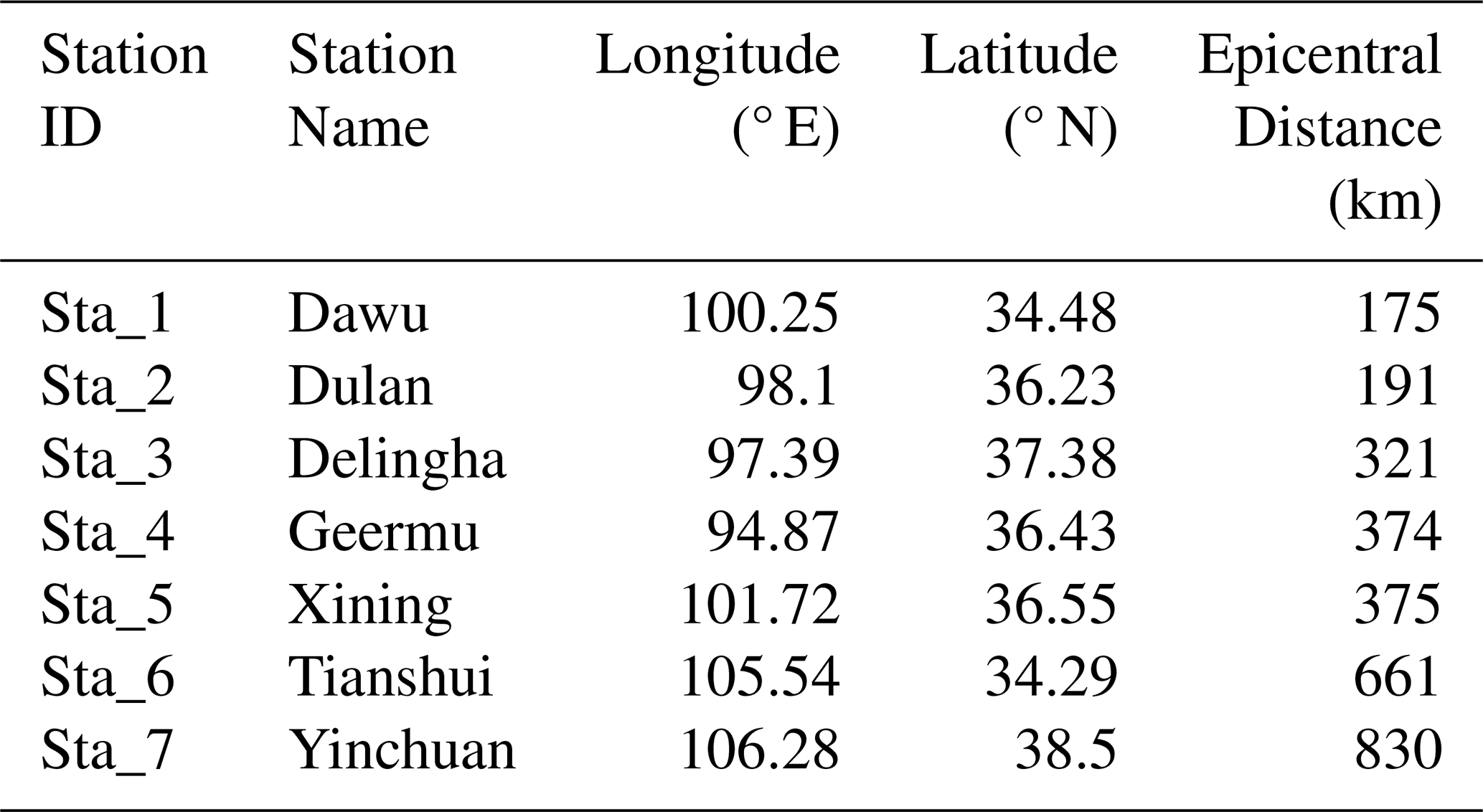
The geomagnetic field data used in this study were obtained from the China Earthquake Administration (https://data.earthquake.cn/index.html, last access: 6 May 2025). All station instruments are GM-4 fluxgate magnetometers or their upgraded variants. The GM-4 fluxgate magnetometer is designed to measure relative variations in three components of the geomagnetic field: the horizontal intensity (H), vertical intensity (Z), and declination (D). For this analysis, 1 Hz magnetic field data were selected. This secondary data at 1 Hz sampling frequency fully retains electromagnetic characteristics in the ultra-low frequency (ULF) range (0.001–0.5 Hz), which holds particular value for seismo-electromagnetic studies (Han et al., 2011). Geomagnetic stations were initially selected with reference to the Dobrovolsky radius D (D = 10^0.43M km, where M is the earthquake magnitude) (Dobrovolsky et al., 1979). Following the exclusion of stations subjected to severe interference (such as from geoelectrical resistivity anomalies, rail transit, or high-voltage direct current power lines) or those with significant data gaps, a total of seven geomagnetic stations were ultimately chosen. Table 1 presents the locations of these stations and their respective epicentral distances.

Table 1 Geomagnetic station information.

2.2 Seismic Event

On 21 May 2021, an M_s 7.4 earthquake struck Madoi County in Qinghai Province, China. The epicenter was located at 34.59° N, 98.34° E, with a focal depth of 10 km (data sourced from the China Earthquake Administration, https://news.ceic.ac.cn/, last access: 13 July 2025). This event stands as the largest earthquake to have occurred on the Chinese mainland since the 2008 M_s 8.0 Wenchuan earthquake. The 2021 Madoi earthquake occurred within the Bayan Har block, situated on the northeastern margin of the Tibetan Plateau, which is one of the most seismically active regions of the Earth (Zhang et al., 2005). Figure 1 shows the epicenter of the 2021 Madoi earthquake and the distribution of the stations.

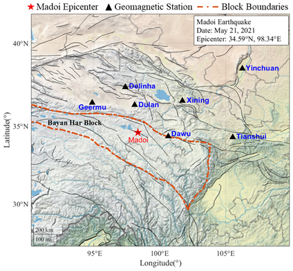
Figure 1 Epicenter of the 2021 Madoi earthquake and distribution of geomagnetic stations. The red star denotes the epicenter, black triangles represent geomagnetic stations, the area enclosed by the orange dashed line is the Bayan Har block, and black lines indicate fault lines (Zhang et al., 2005).

3 Methodology

3.1 Spatially Weighted Non-negative Tensor Factorization

Non-negative Tensor Factorization (NTF) is a technique designed for multilinear dimensionality reduction and feature extraction of non-negative high-dimensional data. After decomposition, it can represent the primary local characteristics of the original data using a reduced amount of data (Hitchcock, 1928; Shashua and Levin, 2001). Applying NTF to decompose the third-order time-frequency spectral tensor enables accurate separation of seismic signals within the dataset. The introduction of coefficient components further allows for the representation of contributions from observation data across different stations to the anomalies. For instance, Fan et al. (2022) constructed a tensor from the magnetic field amplitude spectra of Swarm satellites A and C and employed NTF to extract magnetic field anomalies commonly recorded by both satellites, which may be associated with the 2015 Nepal earthquake. Building upon this, a similar technique was employed to extract fused anomalies in both the magnetic field and electron density recorded by Swarm satellites A and C before the 2021 Madoi earthquake – the same seismic event investigated here (Fan et al., 2024), thereby demonstrating the robustness of NTF in the domain of pre-seismic anomalies extraction. Here, a third-order tensor X ∈ $R^{I\times J\times K}$ from the geomagnetic amplitude spectrum data recorded by multiple stations was constructed. Non-negative Tensor Factorization decomposes the original tensor into a sum of a finite number of rank-1 tensors, expressed as:

$$\begin{array}{}\text{(1)}& \mathbf{X}\approx {\sum }_{r=\mathrm{1}}^R{a}_r\circ b_r\circ c_r=\left[\left[A,B,C\right]\right],\end{array}$$

where, R denotes the rank, indicating the number of features in the decomposition. A ∈ ℝ^I×R is the factor matrix of the first mode (Frequency), B ∈ ℝ^J×R is the factor matrix of the second mode (Time), and C ∈ ℝ^K×R is the factor matrix of the third mode (Space or Station Contribution). The symbol ∘ represents the vector outer product.

During its decomposition process, NTF first randomly initializes the non-negative matrices A, B, and C. The objective function is then used to calculate the discrepancy between the original tensor and the decomposition result. Subsequently, iterative optimization was applied to minimize the objective function and obtain the factor matrices (Hansen et al., 2015). The objective function of traditional Non-negative Tensor Factorization can be expressed as:

$$\begin{array}{}\text{(2)}& \underset{A,B,C\ge \mathrm{0}}{min}{∥X-{\sum }_{r=\mathrm{1}}^R{a}_r\circ b_r\circ c_r∥}_F^{\mathrm{2}}\end{array}$$

where, A = $\left[a_{\mathrm{1}},\mathrm{\dots },a_R\right]\in {\mathbb{R}}^{I\times R}$, B = $\left[b_{\mathrm{1}},\mathrm{\dots },b_R\right]\in {\mathbb{R}}^{J\times R}$ and C = $\left[c_{\mathrm{1}},\mathrm{\dots },c_R\right]\in {\mathbb{R}}^{K\times R}$.

The iterative optimization update rules for NTF follow the Alternating Least Squares (ALS) framework, are derived via gradient descent, and ensure non-negativity (Hansen et al., 2015). Specifically, the update rules are expressed as:

$$\begin{array}{}\text{(3)}& {\displaystyle }A\leftarrow A\odot {\displaystyle \frac{X_{\left(\mathrm{1}\right)}(C\odot B)}{A\left[\left(C^{T}C\right)\odot \left(B^{T}B\right)\right]}},\text{(4)}& {\displaystyle }B\leftarrow B\odot {\displaystyle \frac{X_{\left(\mathrm{2}\right)}(C\odot A)}{A\left[\left(C^{T}C\right)\odot \left(A^{T}A\right)\right]}},\text{(5)}& {\displaystyle }C\leftarrow C\odot {\displaystyle \frac{X_{\left(\mathrm{3}\right)}(B\odot A)}{A\left[\left(B^{T}B\right)\odot \left(A^{T}A\right)\right]}},\end{array}$$

where, ⊙ denotes the element-wise multiplication (Hadamard product), and the division is performed element-wise.

After each iteration, the Karush–Kuhn–Tucker (KKT) conditions are used to determine whether the results have converged (Fan et al., 2022; Chi and Kolda, 2012). The iterative process terminates when either the KKT conditions are satisfied or the maximum number of iterations is reached, yielding the final factor matrices.

In traditional NTF, the decomposition process relies solely on the statistical properties of the data, treating records from all stations equally. However, during decomposition, traditional NTF relies solely on the statistical properties of the data and treats records from all stations equally. This means that global interference signals – such as geomagnetic storms and traveling ionospheric disturbances (TIDs) – which exhibit broad spatial coverage and consistency, are likely to manifest similarly across all stations (Yao et al., 2016; Habarulema et al., 2018). As a result, these interfering signals can be captured within one or a few components, making them difficult to distinguish from seismic anomalies. Furthermore, if certain stations are severely contaminated by noise, their anomalous values may disproportionately influence the global loss function.

Based on the widely accepted observation that seismo-electromagnetic anomalies attenuate with increasing epicentral distance (Wyss, 1997; Hattori, 2004; Schekotov et al., 2007; Han et al., 2014; Xue et al., 2024; Feng et al., 2025), we introduce spatial weighting into the NTF of geomagnetic data. This approach incorporates physical prior knowledge – specifically, the spatial relationship between stations and potential seismic source areas – as a constraint into the decomposition process, which originally relied solely on data statistics. Consequently, the extracted components are not only distinguishable in the time-frequency domain but also more physically meaningful in the spatial domain, thereby enabling more precise isolation of genuine anomaly signals associated with earthquake preparation.

The proposed method is named Spatially Weighted Non-negative Tensor Factorization. It is designed to place greater emphasis on stations near the epicenter, thereby guiding the decomposition process toward a physically more plausible solution space. Specifically, an epicentral distance weight vector for geomagnetic stations is constructed: ω = ${\left[w_{\mathrm{1}},w_{\mathrm{2}},\mathrm{\dots }{w}_K\right]}^T\in R^K$, where w_K represents the weight of the kth station. The weight assignment follows an inverse relationship with the epicentral distance, meaning a smaller distance corresponds to a larger weight. The modified objective function is then formulated as:

$$\begin{array}{}\text{(6)}& \begin{array}{rl}& \underset{A,B,C\ge \mathrm{0}}{min}{∥X-{\sum }_{r=\mathrm{1}}^R{a}_r\circ b_r\circ c_r∥}_F^{\mathrm{2}}\\ & +\mathit{\lambda }{\sum }_{r=\mathrm{1}}^R{∥c_r-\mathit{\omega }∥}_{\mathrm{2}}^{\mathrm{2}}\end{array}\end{array}$$

In the equation, λ denotes the regularization coefficient, while the remaining parameters are consistent with traditional NTF. It is important to note that the regularization term is applied solely to the space (Station Contribution) factor matrix C.

Therefore, in SW-NTF, the update rules for the frequency factor matrix A and the time factor matrix B remain consistent with traditional NTF. However, due to the incorporation of the regularization term for the matrix C, its multiplicative update rule is modified: the denominator includes the positive part of the regularization term's derivative, while the numerator incorporates the negative part. The update rule for the matrix C is given as follows:

$$\begin{array}{}\text{(7)}& C\leftarrow C\odot {\displaystyle \frac{X_{\left(\mathrm{3}\right)}\left(B\odot A\right)+\mathit{\lambda }\mathit{\omega }}{A\left[\left(B^{T}B\right)\odot \left(A^{T}A\right)\right]+\mathit{\lambda }C}}\end{array}$$

The complete procedure of the Spatially Weighted NTF algorithm is summarized as follows:

• 1.

  Initialization: randomly initialize the non-negative matrices A, B, and C.

• 2.

  Iteration: (until convergence or the maximum number of iterations is reached):

  • a.

    Update the frequency factor matrix A (with other factors fixed).

  • b.

    Update the time factor matrix B (with other factors fixed).

  • c.

    Update the space factor matrix C (with other factors fixed and incorporating the spatial regularization).

  • d.

    Calculate the reconstruction error.

• 3.

  Normalization: normalize the column vectors of each factor matrix while preserving their product.

3.2 Data Processing

In this section, a third-order tensor was constructed using 1 Hz observation data of the Z-component from seven geomagnetic stations, and tensor decomposition is performed to extract pre-seismic electromagnetic anomaly signals. Generally, geomagnetic observation data primarily consist of the following components: global magnetic disturbances, local magnetic disturbances (e.g., sources such as anthropogenic noise and meteorological activities), and magnetic signals originating from subsurface activities (Hattori et al., 2013b). To minimize the influence of anthropogenic noise, this study selects and processes Z-component data from local time period of 00:00 to 04:00 LT (Hobara et al., 2004).

Figure 2 illustrates the data preprocessing workflow using the data from 2 May 2021, as an example. Column 1 of Fig. 2a displays the original waveforms of geomagnetic data from seven stations. The data preprocessing pipeline consists of three key stages. First, to eliminate the diurnal variation trend in the geomagnetic data, we employed a 6-level Discrete Wavelet Transform (DWT) with the db5 wavelet basis (Han et al., 2011; Hattori et al., 2013b). The low-frequency background was removed by discarding the approximation coefficients from the final decomposition level, with the result after low-frequency removal shown in the second column of Fig. 2a. Subsequently, to suppress high-frequency noise, multivariate empirical mode decomposition (MEMD) was employed to decompose the data from the seven stations. For each station, the kurtosis and energy entropy of each intrinsic mode function (IMF) were calculated. IMFs with kurtosis > 3 and energy entropy < 0.3 were selected and reconstructed to obtain the denoised signals (Rehman and Mandic, 2010; Liu et al., 2018; Li et al., 2020), as presented in the third column of Fig. 2a. Finally, the Wavelet Synchro-squeezed Transform (WSST) was utilized to obtain the time-frequency amplitude spectrum of the reconstructed data from each station. A third-order non-negative tensor was subsequently constructed using the daily time-frequency amplitude spectra from all seven stations, with its three dimensions representing frequency, time, and station contribution, as illustrated in Fig. 2b.

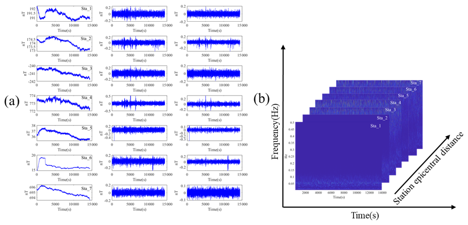
Figure 2 Data preprocessing. In panel (a), the first column displays the original data from the seven stations, the second column presents the detrended signals for each station, and the third column shows the reconstructed signals after high-frequency noise removal using MEMD. Panel (b) illustrates the third-order tensor constructed from the time-frequency amplitude spectra of the seven stations.

We applied the SW-NTF to decompose the daily tensor constructed from the seven stations. The parameters were set as follows: regularization coefficient λ = 0.1, maximum iterations = 200, and convergence tolerance under KKT conditions τ_k = 0.00001. Based on the actual situation that geomagnetic observation data may contain seismic signals, local magnetic disturbances, and global magnetic disturbances, the number of decomposition features R = 3. The decomposition yields three non-negative factor matrices: A = $\left[a_{\mathrm{1}},a_{\mathrm{2}},a_{\mathrm{3}}\right]$ (frequency), B = $\left[b_{\mathrm{1}},b_{\mathrm{2}},b_{\mathrm{3}}\right]$ (time), and C = $\left[c_{\mathrm{1}},c_{\mathrm{2}},c_{\mathrm{3}}\right]$ (station contribution). The three vectors in matrix A represent the spectral characteristics of each component in the geomagnetic data, the three vectors in B depict their temporal variations, and the three vectors in C indicate the contribution of each station to these components.

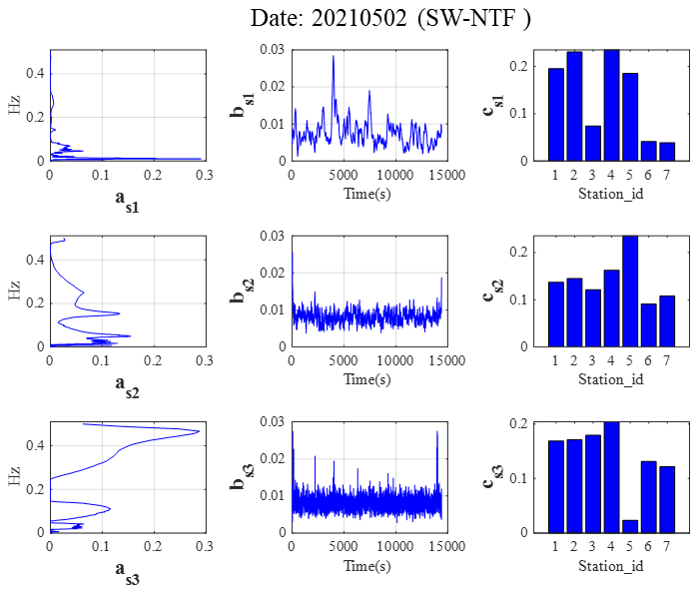
Due to the inherent unordered nature of NTF decomposition results, components potentially associated with seismic activity need to be identified. In previous studies, one of the most frequently reported frequency ranges for seismo-electromagnetic phenomena is 0.01–0.05 Hz (Fraser-Smith et al., 1990; Hayakawa et al., 1996; Hattori et al., 2013a, b; Hayakawa et al., 2023; Han et al., 2014; Hattori, 2004). We defined a frequency ratio coefficient η_r (calculated as the ratio of the energy within the 0.01–0.05 Hz range to the total energy of each vector in the frequency matrix A). The components were then sorted in descending order of this coefficient, resulting in the sequences a_s1(b_s1c_s1), a_s2(b_s2c_s2), and a_s3(b_s3c_s3). The component a_s1(b_s1c_s1) was selected as the seismically relevant component, and its corresponding temporal feature vector b_s1 was subsequently used to extract potential pre-seismic anomalies. The decomposition results for traditional NTF on 2 May 2021 are presented in Fig. 3.

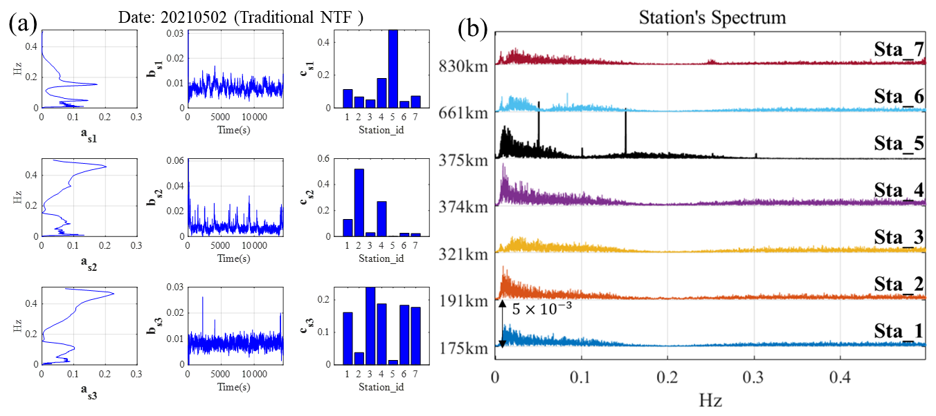
Figure 3 Decomposition results for traditional NTF on 2 May 2021. (a) The three components of traditional NTF decomposition, the first column represents the frequency vector a_s, the second column shows the time vector b_s, and the third column indicates the station contribution vector c_s. (b) Spectra from seven stations on 2 May 2021.

In traditional NTF, the lack of constraints during the decomposition process often leads to unstable results due to random noise in the data or instrument failures at individual stations. For example, in Fig. 3a, the energy of the component considered seismically relevant, a_s1, is predominantly concentrated around 0.05 and 0.15 Hz. Further examination of its corresponding station contribution c_s1 reveals that Sta_5, located farther from the epicenter, dominates this component. As observed in Fig. 3b, the spectrum of Sta_5 exhibits prominent energy peaks at 0.05 and 0.15 Hz, which likely represent far-field interference signals. Clearly, such interference affects the decomposition outcome of conventional NTF. Moreover, in the traditional NTF results, the spectral features a_s2 and a_s3 both show primary energy around 0.45 Hz. The fact that structures with similar spectral characteristics are separated into two distinct components indicates that the conventional method lacks adequate discriminative ability in component separation.

In contrast, the application of SW-NTF yields more satisfactory results. The spatial weighting strategy inherently suppresses the contribution of such noise signals in key components, as the algorithm is designed to identify signal patterns that are prominent in high-weight regions (e.g., near the epicenter) yet faint in low-weight regions, precisely the characteristic of localized seismic anomalies. As shown in Figure 4, in the frequency vector, the energy of a_s1 is primarily concentrated around 0.01 Hz, indicating that potentially earthquake-related anomalies have been effectively extracted. Meanwhile, in the station contribution vector c_s1, several stations closer to the epicenter exhibit similar contribution levels, reflecting spatial consistency. Furthermore, the energy of a_s2 is mainly distributed around 0.05 Hz and 0.15 Hz, while the frequency content of the third component a_s3, is predominantly concentrated near 0.45 Hz. These results demonstrate the superior performance of SW-NTF in signal separation.

Figure 4 Decomposition results for SW-NTF on 2 May 2021.

4 Result

4.1 Temporal Cumulative Results of Geomagnetic Anomalies

Currently, a consensus has yet to be reached within the scientific community regarding the precise temporal window in which pre-seismic magnetic anomalies occur. Previous literature has reported a wide variance in these windows, ranging from several tens of days to a few weeks, or even mere hours prior to the seismic event (Han et al., 2014; Hayakawa et al., 1996; De Santis et al., 2022; Fraser-Smith et al., 1990). According to the empirical law proposed by Rikitake, the duration of precursor activity is proportional to the earthquake magnitude; for events with M_s > 7, geomagnetic anomalies can often be detected several months in advance (Rikitake, 1987). Furthermore, a statistical analysis of global powerful earthquakes conducted by De Santis et al. (2019c) using Swarm satellite data revealed that ionospheric and geomagnetic anomalies typically manifest between 80 and 100 d before the mainshock.

In light of these findings, the present study defines the research interval as the period spanning 90 d before to 30 d after the Madoi earthquake. Daily fused geomagnetic data were structured into tensors and decomposed using SW-NTF, with anomalies subsequently extracted from the time feature matrix B. To enhance detection accuracy, established criteria for identifying seismo-electromagnetic anomalies were adopted, requiring the simultaneous satisfaction of two conditions: the anomaly amplitude must exceed k × σ (where k = 5) and its duration must fall within the range t_min < t < t_max (with t_min = 60 s and t_max = 300 s) (Li and Parrot, 2012, 2013; Zhang et al., 2023). Figure 5 shows the comparison of the cumulative anomalies of the (b_s1) component related to the earthquake before and after the Madoi earthquake with the cumulative anomalies of the other two components (b_s2 and b_s3).

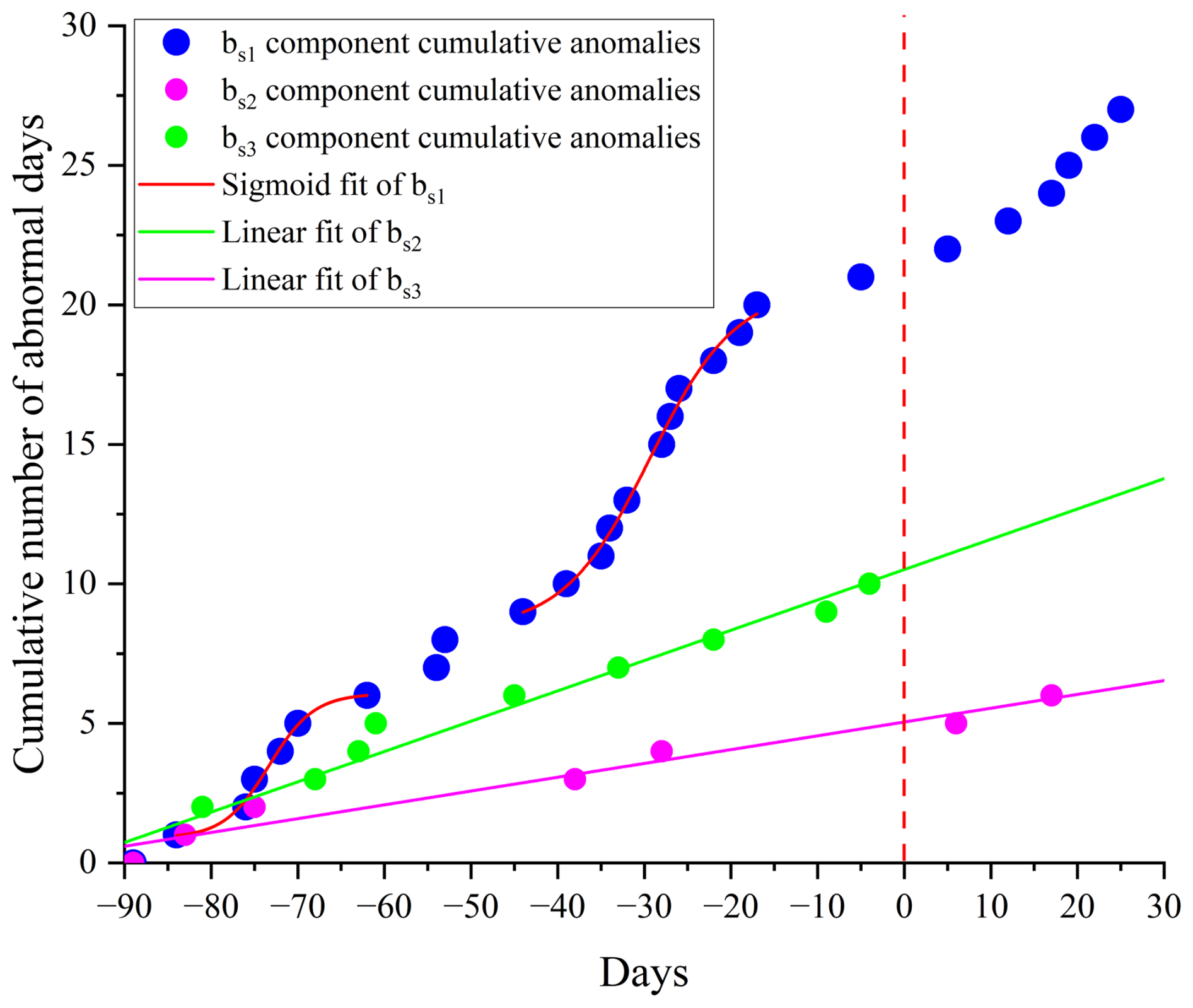
Figure 5 Cumulative anomaly results of the three b_s components from SW-NTF. The red S-shaped curve represents the sigmoidal fit of the non-linear acceleration, while the pink and green solid lines show the linear fitting results for the b_s2 and b_s3 components, respectively. The red dashed line indicates the occurrence time of the mainshock.

In Fig. 5, it is possible to identify two distinct phases of accelerated growth in the earthquake-related b_s1 component before the mainshock. During these periods, geomagnetic anomalies occurred frequently. This observation aligns with numerous previous studies reporting that pre-seismic electromagnetic anomalies often exhibit discontinuous, burst-like, and clustered occurrence patterns (Marchetti et al., 2020a, b; De Santis et al., 2017, 2019b; Marchetti and Akhoondzadeh, 2018; Zhu et al., 2021). A Sigmoid function was employed to characterize these two phases of anomalous acceleration, expressed as:

$$\begin{array}{}\text{(8)}& S_{\mathrm{sigmoid}}\left(t\right)=A_{\mathrm{2}}+{\displaystyle \frac{\left(A_{\mathrm{1}}-A_{\mathrm{2}}\right)}{\left(\mathrm{1}+e^{\frac{(x-x_{\mathrm{0}})}{d_x}}\right)}}\end{array}$$

where A₁, A₂, and d_x represent the lower asymptote, upper asymptote, and time constant, respectively, while x₀ denotes the inflection point – the center of the function where the growth rate reaches its maximum.

The Sigmoid fitting demonstrates high sensitivity to deviations from linear growth patterns. In contrast, the occurrence frequency of anomalies in stochastic systems tends to be stable, resulting in a linear accumulation over time (De Santis et al., 2015, 2017). In other words, an S-shaped growth pattern suggests a potential correlation with seismic activity, whereas a linear growth pattern typically indicates anomalies unrelated to earthquakes.

The first sigmoidal phase was fitted from day −85 to −60, with an inflection point x₀ at −73.3 d and a coefficient of determination R² of approximately 0.98. The second phase was fitted from day −40 to −17, with x₀ = −29.3 d and R² ≈ 0.99. These high R² values indicate excellent fitting performance, confirming that the cumulative anomalies during both nonlinear acceleration phases follow a sigmoidal growth pattern. Conversely, the growth trends of components b_s2 and b_s3 align with linear models, supporting their classification as seismically unrelated components.

Another noteworthy observation is that from approximately 20 d before the earthquake until its occurrence, the cumulative results of the b_s1 component show only very few geomagnetic anomalies. Previous studies have indicated that a period of quiescence often precedes major earthquakes worldwide (Wyss et al., 1997; Gentili et al., 2019). Similar observations have been demonstrated in laboratory experiments, where a brief cessation of acoustic emission signals was observed prior to rock failure, this phenomenon has been attributed to the concept of dilatancy hardening in the region surrounding an impending earthquake (Scholz, 1988). These findings suggest that the temporal variation of pre-seismic anomalies may be linked to the preparation process of the Madoi earthquake.

For comparison, the anomalies extracted by traditional NTF were accumulated to obtain Fig. 6. Specifically, around 70 d before the earthquake, a phase of acceleration is observed, followed by another between days −30 and −20. However, compared to SW-NTF, these acceleration phases are less pronounced and progress more gradually. During the remaining periods, the cumulative trend remains predominantly linear. Overall, the cumulative anomalies from traditional NTF exhibit a linear growth pattern, with a coefficient of determination (R²) of approximately 0.97 for the linear fit. This indicates that our proposed SW-NTF appears to be more effective in extracting pre-seismic electromagnetic anomalies.

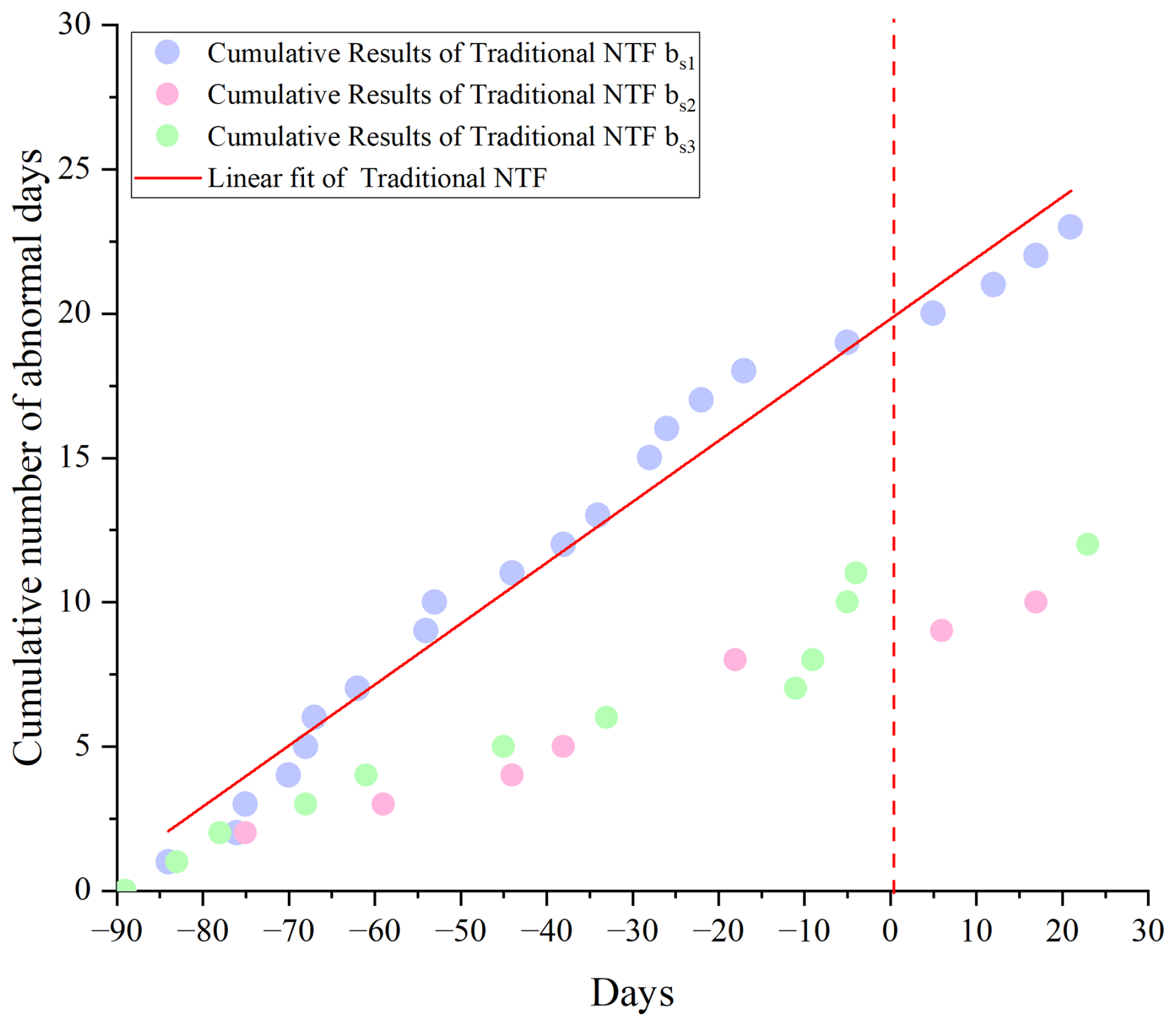
Figure 6 Temporal cumulative anomaly results from traditional NTF. The red solid line shows the linear fit to the cumulative anomalies obtained by traditional NTF, and the red dashed line marks the occurrence time of the mainshock.

4.2 Spatial Characteristics of Geomagnetic Anomalies

Beyond the analysis of temporal characteristics, the spatial evolution of geomagnetic anomalies before the earthquake was also investigated. The station contribution matrix in SW-NTF enables us to reflect the contribution of each station's observational data to the daily fused geomagnetic anomalies. Based on the station contribution matrix C obtained from the daily decomposition results, the stations that make primary contributions can be identified. This allows us to illustrate the spatial evolution of pre-seismic anomalies and investigate the earthquake preparation process, as shown in Fig. 7.

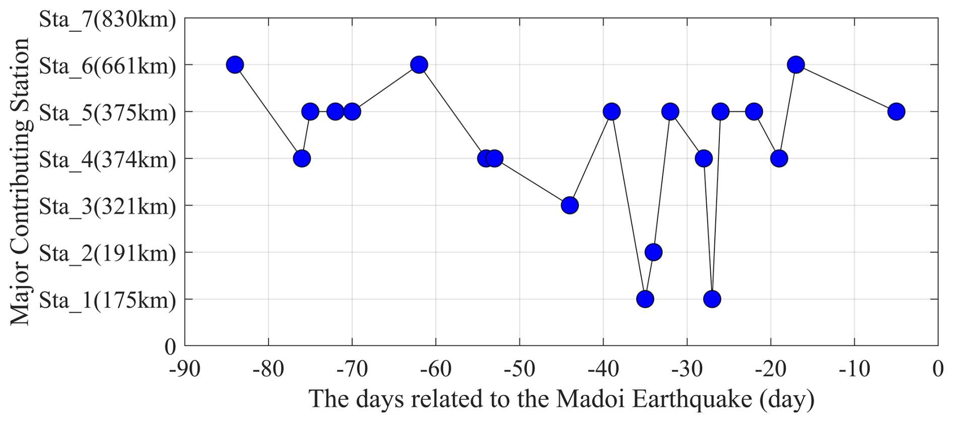
Figure 7 Temporal Variation of Primary Contributing Stations in the geomagnetic anomalies before the 2021 Madoi earthquake.

From approximately day −90 to day −27, a clear spatial migration pattern is observed: the station with the maximum contribution coefficient gradually shifts from those farther from the epicenter to those closer to it, with all maximum contribution coefficients ranging between 0.4 and 0.7. This indicates that during this phase, the spatial location of the dominant station in the anomalies progressively migrated toward the epicenter. However, beginning about 1 month before the earthquake, the stations exhibiting the maximum contribution were exclusively located beyond approximately 350 km from the epicenter, with no stations near the epicenter showing dominant contributions. The distinct difference in spatial evolution between these two phases may reflect changes in subsurface stress. Moreover, in existing studies on the pre-seismic period of the Madoi earthquake, similar temporal patterns of quiescence were observed in thermal anomaly parameters, such as the Microwave Brightness Temperature (MBT) and Outgoing Longwave Radiation (OLR), within the epicentral area (Jing et al., 2022; Liu et al., 2023; Yang et al., 2025). Ma and Guo (2014) suggest that in heterogeneous media, faults contain both weak and strong segments. During the initial stage of stress loading, micro-fracturing and slip tend to occur in the relatively weak zones – often at the edges of the seismogenic area – releasing stress. As stress continues to accumulate and concentrate on the strong, locked segments, the fault enters a locked phase, making a large earthquake inevitable. This model is largely consistent with our observed spatiotemporal changes in pre-seismic anomalies: geomagnetic anomalies first migrate toward the epicenter, followed by a period of quiescence in the epicentral area, after which the mainshock occurs.

5 Discussion

5.1 Analysis of Space Weather Impacts

Since seismo-geomagnetic observations are susceptible to interference from magnetic storms and solar activity, the space weather conditions during the study period were investigated. The Dst and ap indices were used to assess geomagnetic activity levels (data sourced from the World Data Center for Geomagnetism, Kyoto, https://wdc.kugi.kyoto-u.ac.jp/, last access: 29 July 2025). Based on the classification criteria for Dst proposed and the standard classification for the ap index by Loewe and Prölss (1997), and relevant experience in earthquake studies (Yao et al., 2016), geomagnetic activity intensity was categorized into three levels, ranging from weak to strong. The geomagnetic activity levels corresponding to the periods with observed anomalies are summarized in Table 2.

Table 2 Number of anomalies under different geomagnetic conditions.

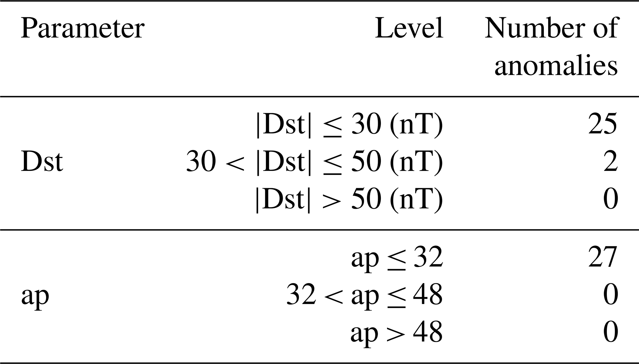
The results indicate that the observed geomagnetic anomalies occurred almost exclusively during periods of low geomagnetic activity, with only two exceptions under moderate activity levels. This result demonstrates that the anomalies are independent of strong geomagnetic disturbances, implying that the seismically relevant anomalies extracted by SW-NTF are not caused by intense space weather events. Therefore, it can be concluded that SW-NTF is capable of extracting geomagnetic anomalies potentially related to seismic processes.

5.2 Frequency Characteristics of Geomagnetic Anomalies

In this section, the frequency characteristics of the anomalies and their relationship with the seismic source were investigated. The frequency characteristics are obtained by identifying the dominant frequency from frequency features a_s1 form frequency matrix A. The frequency variations of the pre-earthquake anomalies are presented in Fig. 8.

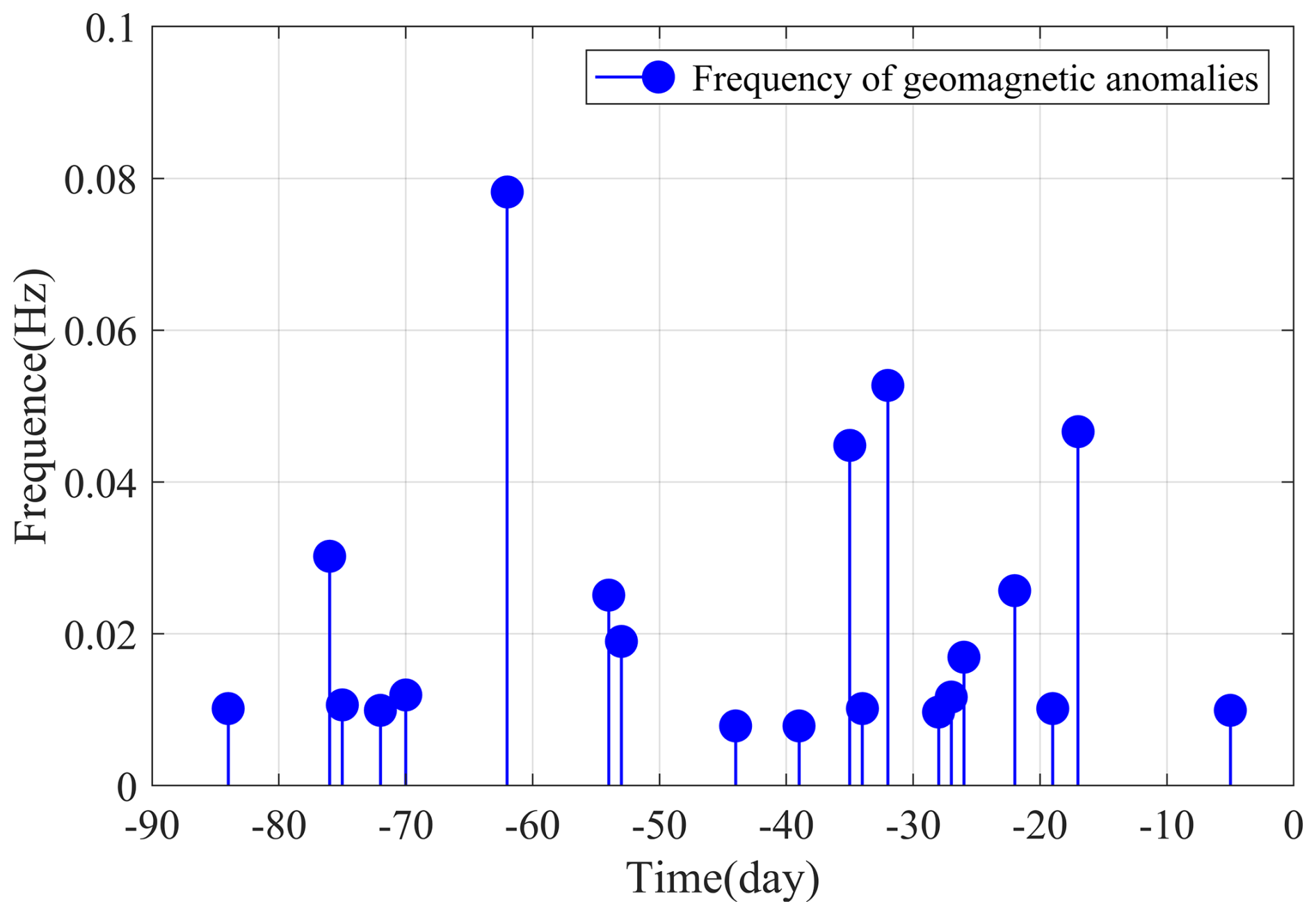
Figure 8 Frequency characteristics of geomagnetic field anomalies before the 2021 Madoi earthquake.

As shown in Fig. 8, the pre-earthquake geomagnetic field anomalies exhibit frequencies ranging from 0.007 to 0.08 Hz, with most concentrated around 0.01 Hz. Interestingly, Fan et al. (2024) reported that the frequency distribution of ionospheric magnetic field anomalies prior to the 2021 Madoi earthquake, as observed by Swarm satellites, fell within the range of 0.015–0.06 Hz, which closely aligns with the frequency range of the geomagnetic field anomalies identified in this study.

The focal depth of the geomagnetic anomalies was estimated using the electromagnetic skin depth formula, which is expressed as follows (Ouyang et al., 2020):

$$\begin{array}{}\text{(9)}& \mathit{\delta }=\sqrt{\mathrm{1}/\left(\mathit{\pi }f\mathit{\mu }\mathit{\sigma }\right)}\end{array}$$

In the formula, f denotes the frequency, and μ is the magnetic permeability, where the permeability of free space μ₀ = $\mathrm{4}\mathit{\pi }\times {\mathrm{10}}^{-\mathrm{7}}$ H m⁻¹ is adopted. The electrical conductivity σ is taken as σ ≈ 1/10–1/2 S m⁻¹ (Zhan et al., 2021).

Using Eq. (9), the estimated anomaly depth δ ranges from approximately 10.62 to 15.01 km, which is comparable to the subsurface rupture depth of 10–15 km in the epicentral region of the 2021 Madoi earthquake (Wang et al., 2022). Therefore, it can be hypothesized that the extracted pre-earthquake geomagnetic field anomalies are associated with the 2021 Madoi earthquake.

5.3 Temporal Variations in the Amplitude of Geomagnetic Anomalies and Potential Mechanisms

In addition to analyzing the frequency characteristics of pre-seismic anomalies, variations in the amplitude of the anomalies before the earthquake were also examined. The anomaly amplitude was obtained by reconstructing the time-domain signal from the seismically relevant component b_s1 (a_s1 and c_s1), with the results presented in Fig. 9.

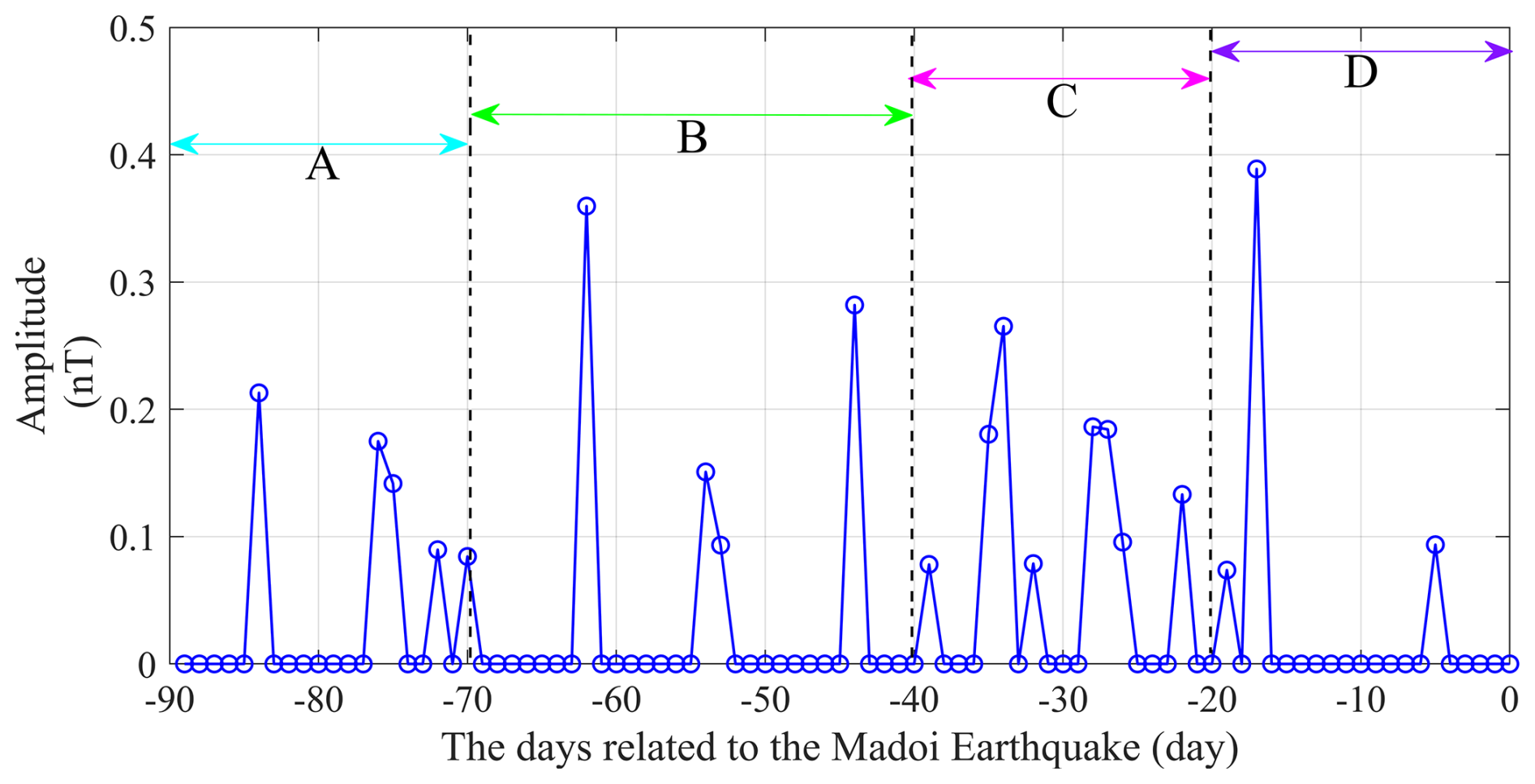
Figure 9 Temporal variation in the amplitude of geomagnetic fusion anomalies before the Madoi Earthquake. The blue curve represents amplitude variation.

Overall, the magnitude of pre-earthquake geomagnetic anomalies ranged between 0.1 and 0.4 nT, which corresponds to the widely reported range of pre-earthquake magnetic field anomaly variations (Marchetti and Akhoondzadeh, 2018; Kelley et al., 2017; Utada et al., 2011). The amplitude of the pre-seismic geomagnetic anomaly exhibits an increasing trend. Multiple peaks occur before the earthquake, with their magnitudes rising progressively. Approximately −18 d, the amplitude of the anomaly reaches its maximum. This phenomenon may indicate that the source region underwent a nonlinear, intermittent process of stress accumulation and electromagnetic radiation release during the impending seismic stage. We suggest that this periodic anomaly pattern, characterized by accelerating amplitude growth, could represent an electromagnetic manifestation of the fault system transitioning into a critical state before instability. He et al. (2023) experimentally analyzed rock magnetic field characteristics at different loading stages, and similar variations were found in the pre-seismic magnetic anomalies extracted herein. During the initial compaction phase A (−90 to −70 d in Fig. 9), the magnetic induction intensity fluctuates and increases. In this stage, the magnetic field is mainly produced by current variations caused by inter-granular friction and the slip-rubbing along primary pores and fractures within the rock. In the elastic deformation phase B (−70 to −40 d), the magnetic induction intensity shows a steadily increasing trend, with the magnetic field primarily generated by the piezoelectric polarization current effect. During the crack propagation phase C (−40 to −20 d), the initiation and growth of internal cracks, along with associated frictional slip, produce varying currents, leading to a rapid increase in magnetic induction intensity. Here, the magnetic field results not only from a minor contribution of the piezoelectric effect, but is mainly attributed to frictional current effects and crack-extension current effects. The anomaly amplitude at this stage approaches 0.2 nT, this experimental result aligns with the theoretical value obtained by Venegas-Aravena et al. (2019), indicating that when fractures form in the semi-brittle-ductile zone (depth 10–20 km), the magnetic field increases by approximately 0.2 nT. In the failure phase D (from about −20 d until the earthquake occurs), a large number of micro-cracks propagate, intersect, and coalesce rapidly within the rock, eventually connecting to form visible macroscopic cracks. The magnetic induction intensity rises sharply during this stage; the greater the number of cracks and the faster their propagation, the larger the induced current. It should be emphasized that although the time scale of our observational period (90 d) cannot be directly matched with the duration of the rock experiment (approximately 200 s), and the preparation period for actual earthquake magnitudes may be considerably longer, ranging from several months to years (Scholz et al., 1973), the trend of magnetic field variations observed in the laboratory experiment can still be used to examine the plausibility of the pre-seismic magnetic anomalies identified in our study.

5.4 Comparative Analysis with Cumulative Benioff strain

Pre-seismic electromagnetic anomalies originate from subsurface processes. To investigate the correlation between the extracted anomalies and seismic activity, the temporal cumulative characteristics of the pre-seismic electromagnetic anomalies were compared with those of lithospheric seismicity. The earthquake catalog is sourced from the China Earthquake Administration (https://news.ceic.ac.cn/, last access: 13 July 2025), covering an area within ±2° from the epicenter, which corresponds to approximately a 400 km rupture zone for the 2021 Madoi earthquake (Li et al., 2025). The cumulative Benioff strain is used to describe the incremental strain rebound occurring on faults within the study area (Benioff, 1949; De Santis et al., 2015). The formula for calculating the cumulative Benioff strain S is as follows:

$$\begin{array}{}\text{(10)}& S\left(t\right)=\sum _{i=\mathrm{1}}^{N\left(t\right)}\sqrt{{\mathrm{10}}^{\mathrm{4.8}+\mathrm{1.5}{M}_i}}\end{array}$$

where M_i is the magnitude of the ith earthquake and N(t) is the total number of earthquakes until time t.

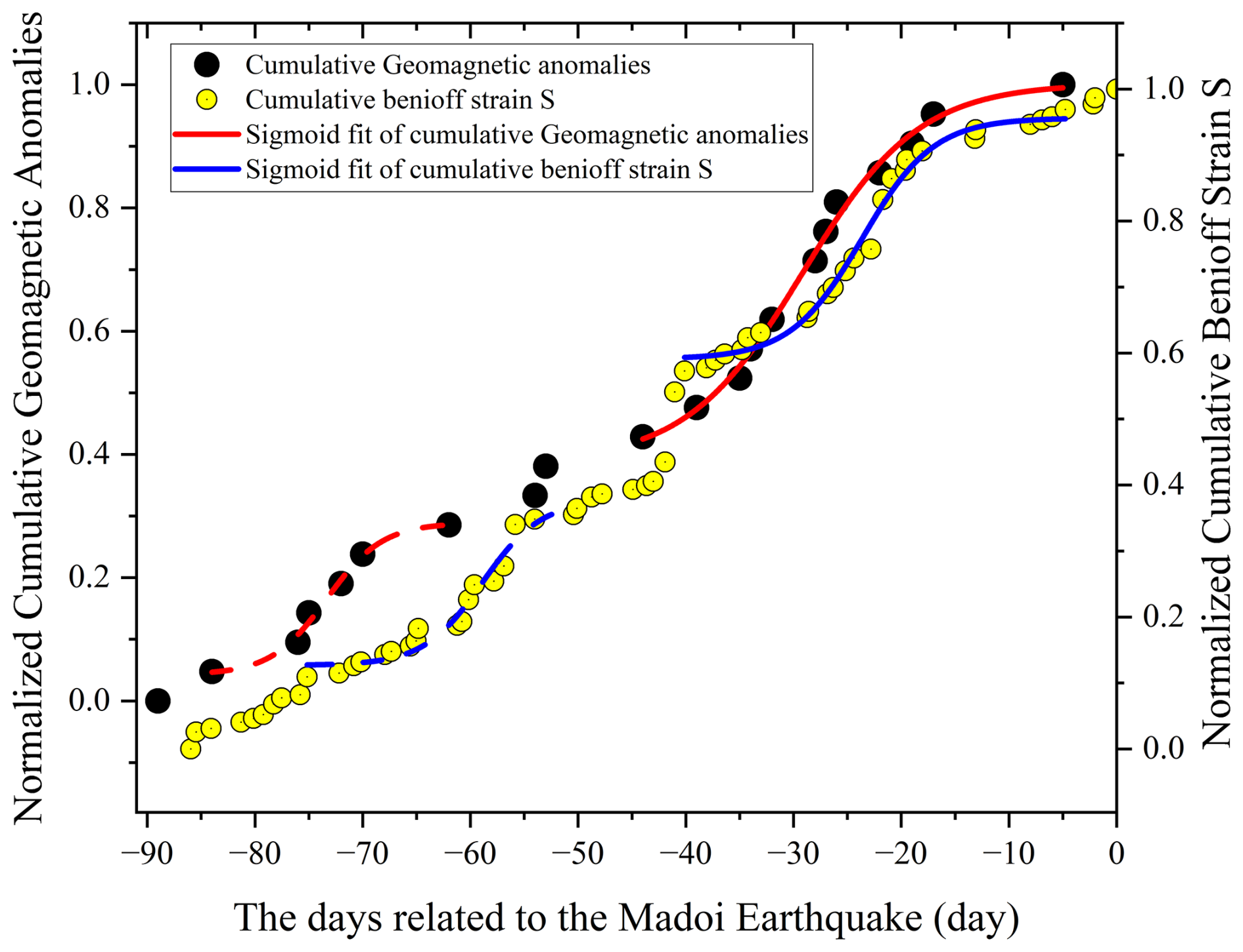
Figure 10 Comparison between cumulative geomagnetic anomalies and cumulative Benioff strain. Black dots represent cumulative geomagnetic anomalies, yellow dots denote cumulative Benioff strain, red and blue curves show the sigmoidal fits for the geomagnetic anomalies and cumulative Benioff strain, respectively. Dashed lines indicate the first acceleration phase, while solid lines represent the second acceleration phase.

Before large earthquakes, an increase in small earthquake rate is often observed (Brace and Byerlee, 1966). However, due to the limited detection capability of seismic networks, some smaller-magnitude events may go unrecorded. Therefore, it is necessary to determine the completeness magnitude M_c, which represents the minimum magnitude that can be fully detected within the study region. M_c was estimated using the maximum curvature method (Wiemer and Wyss, 2000), yielding a value of 0.71. Subsequently, shallow-focus earthquakes with focal depths less than 50 km were selected from the catalog to calculate the cumulative Benioff strain S. The temporal variations of the cumulative geomagnetic anomalies and the cumulative Benioff strain in the lithosphere are shown in Fig. 10.

In Fig. 10, the cumulative Benioff strain exhibits two distinct phases of accelerated growth. Similarly, the sigmoid function was applied to fit these phases. The first phase, spanning approximately from day −75 to −50 (depicted by the blue dashed sigmoidal curve in the figure), has a coefficient of determination (R²) of about 0.96. The second phase, from approximately day −40 to −5 (represented by the blue solid sigmoidal curve), shows an R² of approximately 0.99. The consistency of these two accelerated growth phases across both geophysical datasets suggests the existence of two critical stages before the mainshock. This observation aligns with the findings of Ma and Guo (2014), indicating the possible occurrence of a meta-instability stage and two unstable fault deformation stages before the seismic event.

It is noteworthy, however, that in both phases, the acceleration of geomagnetic anomalies preceded that of the cumulative Benioff strain by approximately 5 to 15 d. This temporal offset can be attributed to the fact that Benioff strain primarily reflects macroscopic-scale rock rupture and slip. Significant acceleration in strain rate occurs only when a substantial number of microcracks have formed, propagated, and interconnected. In contrast, systematic changes in the microscopic physical properties (such as magnetic and electrical characteristics) of rocks in the source region already take place before crustal stress accumulates sufficiently to generate a notable macroscopic rupture (manifested as accelerated Benioff strain).

In Scholz's dilatancy-diffusion model, it is proposed that dilatancy initiates when the stress reaches approximately half the rock's fracture strength, a stage characterized by the nucleation and growth of microcracks (Scholz et al., 1973). Molchanov and Hayakawa suggested that charge separation occurs on the opposing surfaces of newly formed microcracks, generating transient currents and emitting electromagnetic waves (Molchanov and Hayakawa, 1995). The generation of such microcracks alters the pore structure and connectivity of the rock, thereby affecting resistivity and subsequently leading to magnetic anomalies (Xue et al., 2014). In summary, geomagnetic anomalies capture signals indicating that “the rock has begun to be damaged”, whereas the acceleration of Benioff strain reflects the process whereby “the damage has accumulated to a certain extent and begins to propagate”. Therefore, the extracted geomagnetic anomalies may serve as precursors either to the 2021 Madoi earthquake or to the trend of small-scale seismic activity preceding the mainshock.

5.5 Spatiotemporal Correlation Between Geomagnetic Anomalies and Seismological b value

Existing studies have demonstrated that the b value reflects the magnitude-frequency distribution of earthquakes within a specific region and serves as an indicator of the subsurface stress state. An observed decrease in b value before seismic events is widely regarded as a manifestation of increasing stress accumulation (Scholz, 1968; Schorlemmer et al., 2005). The seismological b value is derived from the Gutenberg–Richter law: log N = a−bM, where M represents the earthquake magnitude, and N denotes the number of earthquakes with magnitudes greater than M. This relationship is commonly referred to as the G–R relation (Gutenberg and Richter, 1944). An increase in the b value indicates a higher rate of occurrence for smaller seismic events. The b value was calculated using the maximum likelihood estimation method (Aki, 1965):

$$\begin{array}{}\text{(11)}& b={\displaystyle \frac{\mathrm{1}}{\ln \left(\mathrm{10}\right)\left(\stackrel{\mathrm{‾}}{M}-M_{\mathrm{C}}\right)}}\end{array}$$

where $\stackrel{\mathrm{‾}}{M}$ is the average magnitude of all earthquakes in the target catalog sample with magnitudes greater than M_C, and M_C represents the minimum completeness magnitude. The confidence interval for the b value can be estimated using equation:

$$\begin{array}{}\text{(12)}& {\mathit{\sigma }}_b={\displaystyle \frac{b}{\sqrt{N}}}\end{array}$$

where N represents the total number of events in the given sample.

Finally, the b values for the period spanning 90 d before the earthquake were calculated within a ±7° range around the epicenter, using a 3 d moving window with a 1 d step and setting a minimum of 20 seismic events. Figure 11 illustrates the relationship between the cumulative geomagnetic anomalies and the temporal characteristics of the pre-seismic b values.

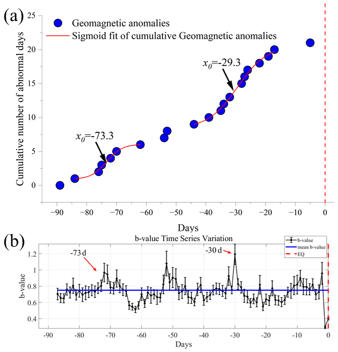
Figure 11 Comparison of temporal variations between geomagnetic anomalies and b values. (a) Temporal cumulative results of geomagnetic anomalies, with the S-shaped curve representing the sigmoidal fit. (b) Temporal variation of b values, where the blue line indicates the mean b value. The red dashed line marks the mainshock.

Figure 11a shows that the inflection points x₀ of the two S-shaped growth phases for the geomagnetic anomalies are located at −73.3 and −29.3 d, respectively. The inflection point in a sigmoidal fit is generally considered to correspond to a critical point in a non-random system: as this point is approached, anomalies accelerate, and the rate of increase decelerates thereafter (De Santis et al., 2019a). In Fig. 11b, it can be observed that during the two phases of accelerated geomagnetic anomaly growth, the pre-seismic b value exhibits similar variations. Specifically, from day −80 to −60, the b value first rises and then falls, peaking at day −73. From day −40 to −20, it reaches its maximum around day −30. An increase in b value indicates enhanced release of stress through a higher frequency of seismic events. The temporal coincidence between the inflection points of the two anomaly acceleration phases and the peaks in b-value variation suggests that SW-NTF is capable of extracting geomagnetic anomalies related to seismic activity.

Furthermore, the spatial variation of b values in the epicentral region was computed at 30 d intervals. The region was first divided into 0.1° × 0.1° grids. The b value was then calculated for each grid within a spatial window of 5 × 5 grids centered on the target grid, requiring a minimum of 20 seismic events within each window. The resulting b value was assigned to the corresponding grid cell to map the spatial variation (Chen et al., 2022b).

Based on Fig. 12, the following spatiotemporal evolution pattern can be observed. From day −90 to −60, the b value in the area southwest of the epicenter was relatively high compared to other regions, indicating a stress release zone. During days −60 to −30, the b values northeast of the epicenter exceeded 1.0, accompanied by frequent small earthquakes. Furthermore, from day −90 to −30, the strain release areas in the periphery of the epicenter expanded rapidly, became interconnected, and progressively engaged the entire fault zone (Ma and Guo, 2014). Consequently, the geomagnetic anomalies during this period were primarily contributed by stations distributed across this extensive region. From day −30 until the earthquake occurrence, stress release in the peripheral areas led to continuous stress accumulation in the epicentral region (Noda et al., 2013), with b values dropping below 0.5. This signifies the locking of the epicentral area and marks the transition of the earthquake preparation into an irreversible stage. Accordingly, fewer anomalies were detected during this phase. Following the mainshock, the b values began to recover as stress was released. This finding further demonstrates that the geomagnetic anomalies extracted in this study are associated with anomalous subsurface stress changes and may contain precursory information related to the 2021 Madoi earthquake.

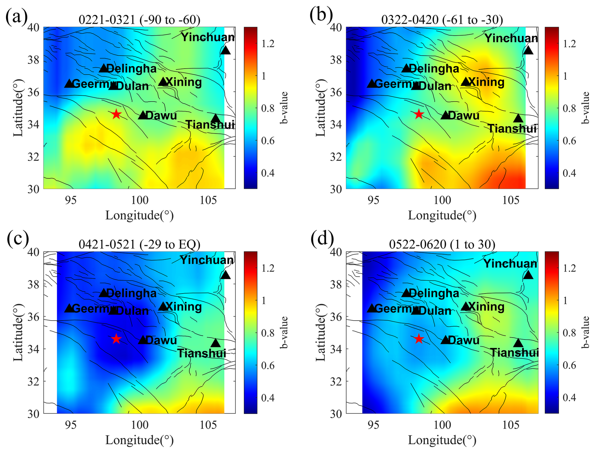
Figure 12 Spatial distribution of pre-seismic b values. The four subpanels show the spatial variation of b values over consecutive 30 d intervals, spanning from 90 d before to 30 d after the earthquake. The star denotes the epicenter, black triangles represent geomagnetic stations, and black lines indicate faults.

6 Conclusion

To address the limitation of traditional NTF, which performs inadequately in decomposing geomagnetic station data due to the lack of prior information, a SW-NTF method is proposed in this study for extracting fused pre-seismic magnetic anomalies from multi-station observations. Using this improved approach, the geomagnetic anomalies preceding the 2021 M_s 7.4 Madoi earthquake are investigated, based on 1 Hz Z-component data recorded at seven stations spanning from 90 d before to 30 d after the mainshock. A third-order tensor was constructed daily from the multi-station data and subsequently decomposed using SW-NTF to extract pre-seismic geomagnetic anomalies. The spatiotemporal characteristics of the extracted anomalies were analyzed and compared with those obtained from traditional NTF. Furthermore, the correlation between the anomaly frequency and the seismic source was examined. Subsequently, the potential influence of geomagnetic activity on the detected anomalies was examined. Furthermore, the variation characteristics of the pre-seismic geomagnetic anomalies were comparatively analyzed using magnetic field changes observed in rock loading experiments. In addition, the association between the geomagnetic anomalies and seismic activity was investigated by comparing the temporal cumulative characteristics of Benioff strain and the spatiotemporal distribution of seismological b values with the extracted anomalies. The main findings are summarized as follows:

• 1.

  Compared to conventional NTF, SW-NTF introduces constraints based on station spatial locations into the optimization process. This enables it to more effectively separate signal components originating from the source region that exhibit clear spatial decay characteristics from the background field. As a result, SW-NTF may more directly correlate with the physical processes at the seismic source and improves the robustness of geomagnetic anomaly extraction.

• 2.

  The pre-seismic geomagnetic anomalies extracted by the SW-NTF method exhibit two phases of S-shaped accelerated growth in the time domain, occurring from day −85 to −60 and from day −40 to −17, respectively. Spatially, the anomalies initially appeared at stations farther from the epicenter and gradually migrated toward and clustered at stations closer to the epicenter.

• 3.

  The variation characteristics of pre-earthquake magnetic field anomalies correspond well with the magnetic field variation characteristics observed in rock loading experiments.

• 4.

  The accelerated phases of the pre-seismic geomagnetic anomalies correspond well, in both time and space, with periods of frequent seismic activity during stress release stages. In addition, the quiescence of anomalies immediately before the mainshock appears to be associated with the locking of the seismogenic zone during the preparation process of the 2021 Madoi earthquake.

Several limitations of this work should be acknowledged when interpreting the findings. One limitation of this study stems from the spatial distribution of the currently available geomagnetic stations is suboptimal, characterized by a lack of stations within 100 km of the epicenter and a concentration predominantly on the northern side of the epicenter. Another limitation concerns the relatively short time window analyzed in this study. The conclusions drawn are based on data from a limited period; therefore, they may not capture the full spectrum of long-term deformation processes or the complexities of the seismic cycle.