Early identification of reservoir-bank landslides in deeply incised mountain canyon areas with interferometric baseline optimization

The complex geological conditions in deeply incised mountainous canyon areas make reservoir-bank landslides a frequent hazard. Accurate interferogram selection and baseline network configuration are crucial for SBAS-InSAR-based landslide monitoring, yet are severely challenged by seasonal vegetation decorrelation. To overcome this limitation, this study proposes a novel Vegetation-Adaptive WCTM that integrates time-series vegetation dynamics into interferometric baseline optimization. This approach establishes a vegetation–coherence coupling model to dynamically adjust coherence thresholds based on quantified vegetation coverage levels and synergizes ERA5 meteorological data with tropospheric delay modeling for atmospheric correction. The results demonstrate significant advancements: (1) The deformation rate standard deviation is reduced by 0.520 and 0.192 compared to traditional short-temporal baseline and average coherence threshold methods, respectively, corresponding to a 29.1 % improvement (1.2668 vs. 1.7865). (2) The proposed method improves phase-unwrapping robustness and the spatial continuity of the deformation field under vegetation-induced decorrelation, thereby enhancing landslide detectability in densely vegetated canyon slopes, particularly during low-coherence vegetation seasons. (3) 39 landslides were successfully identified, representing a 22 % increase compared to conventional methods (32 landslides), with 7 new high-risk sites discovered even during low-coherence vegetation seasons. Based on field verification with drone surveys, typical landslides were selected to analyze their spatial distribution and temporal evolution patterns, demonstrating the applicability of the method in deeply incised mountainous canyon areas. These findings provide theoretical and technical support for regional disaster prevention and mitigation efforts.

1 Introduction

Landslides along reservoir banks are a common geological hazard during the construction and operation of hydraulic and hydropower engineering projects (Liu et al., 2022; Li et al., 2021). These landslides are typically concentrated on the steep slopes on both sides of deeply incised mountain canyon reservoir banks (Zhu et al., 2024; Lu et al., 2019). Early identification of reservoir-bank landslides is a crucial component of geological hazard prevention and risk assessment.

Traditional technologies, such as Global Navigation Satellite Systems (GNSS) (Guo et al., 2025; Mao et al., 2024) and optical remote sensing (Cai et al., 2024; Guo et al., 2016), are unable to meet the current demands for landslide detection. In contrast, Synthetic Aperture Radar Interferometry (InSAR) has shown significant potential (Li et al., 2020; Zhou et al., 2022). Deformation monitoring technology based on InSAR baseline optimization has become a key method for high-precision early landslide identification (Ferretti et al., 1999; Pepe, 2021; Liao et al., 2021). However, SBAS-InSAR technology requires high-quality interferograms and a well-constructed baseline network. Incorrect or inaccurate selection of interferograms and baseline network configurations may introduce decorrelation errors and systematic errors, reducing the accuracy of deformation inversion or even preventing correct inversion of deformation results (Zebker and Pepin, 2021; Zhang et al., 2022). Additionally the accuracy of landslide monitoring is influenced by multiple factors, such as decorrelation caused by complex terrain, coherence fluctuations due to land cover changes, and the rational configuration of interferometric baseline optimization parameters (Liu et al., 2024; Ren et al., 2022; Wang et al., 2023; Zhang et al., 2022). Selecting high-quality interferograms and optimizing the interferometric baseline network in the extreme natural conditions of deeply incised mountain canyon regions has become an important research topic for large-scale reservoir bank landslide identification and monitoring.

Currently, the methods for interferogram selection and baseline optimization can generally be divided into three categories: The first category is expert knowledge-based manual selection of interferograms. In this approach, expert knowledge is used to conduct empirical analysis of all acquired interferograms. The interferograms with higher coherence are selected through manual judgment based on coherence comparisons. For example, Shi et al. (2021) manually selected interferograms with higher coherence based on empirical knowledge to study the surface response and underground characteristics during the groundwater extraction restriction period in Suzhou. Although this method can effectively reduce the impact of spatiotemporal decorrelation in forested areas with extremely low coherence, it is highly subjective due to reliance on expert knowledge, and is time-consuming and labor-intensive. Additionally, it fails to meet the deformation monitoring requirements for long-term time-series landslide detection in large-scale reservoir banks.

The second category of methods involves selecting interferograms by simultaneously setting temporal baseline and spatial baseline thresholds. During the SBAS-InSAR processing, interferograms are selected based on short time baseline and spatial baseline thresholds, which are determined through pre-experimental comparative analysis or prior knowledge. For example, Zhao et al. (2012) used ALOS PALSAR2 data for large-scale landslide detection in Southern California and Oregon, while Zhou et al. (2023) utilized Sentinel-1 data to monitor permafrost changes in the XiaoTuo River region, both of which set short time and space baseline thresholds for interferogram selection. Although setting short time and spatial baseline thresholds is the most widely used method for interferogram selection, this approach is based on the empirical assumption that ground objects undergo minimal changes over short time intervals, which will not induce spatiotemporal decorrelation (Li and Hong, 2020). However, this assumption does not guarantee that all interferogram pairs will exhibit good coherence. On the contrary, setting excessively short time and spatial baseline thresholds can introduce decorrelation and systematic errors, reducing the accuracy of deformation inversion results.

The third category of methods is based on coherence coefficient for interferogram selection, where interferograms are chosen by setting a coherence coefficient threshold and optimizing the interferometric baseline network. For example, Tao et al. (2021) used a custom coherence coefficient threshold for interferogram selection; Wang et al. (2022, 2023) directly used the average coherence between SAR images as a baseline constraint indicator to optimize interferogram selection; Zhang et al. (2024) used average segmented coherence threshold coefficients to select interferograms in landslide creep identification and monitoring in the Xiaojiang River Basin. The coherence coefficient of InSAR interferograms is influenced by the spatiotemporal baseline of SAR images and external environmental coupling, which can accurately reflect the quality of the interferogram. Setting a coherence coefficient threshold is a reliable method for generating a robust interferometric baseline network. Custom coherence coefficient thresholds are often established through prior knowledge or comparative pre-experiments. However, this method is highly subjective and suffers from issues such as insufficient interferogram samples for pre-experiments. Moreover, the set thresholds cannot account for the intermittent coherence problems caused by vegetation changes, while the average coherence coefficient threshold overly relies on simple statistical patterns and fails to consider the impact of vegetation cover changes on the coherence of interferograms.

In summary, compared to other interferometric baseline optimization methods, expert knowledge-based manual selection of interferograms is the most time-consuming and labor-intensive approach, making it unsuitable for long-term landslide deformation monitoring along reservoir banks. Although methods based on simultaneous setting of temporal/spatial baseline thresholds and those using coherence coefficient for interferogram selection have improved upon traditional expert-based approaches, these methods remain highly subjective and fail to cover all potential baseline selection errors. They may also introduce decorrelation and systematic errors, thereby affecting the accuracy of deformation inversion and limiting their applicability in complex environments. Furthermore, they inadequately account for the impacts of external environmental conditions on coherence (Dai et al., 2022; Westerhoff and Steyn-Ross, 2020; Zhang et al., 2023). For instance, the application of InSAR in low-coherence areas such as mountainous canyon regions and vegetated zones faces considerable limitations (Lemmetyinen et al., 2022). The combination of temporal and spatial baselines is critical in deformation monitoring; ideally, baseline combinations should maintain high coherence while ensuring the precision of deformation signal extraction. However, certain temporal and spatial baseline combinations may exhibit superficially high coherence but result in distortion of deformation information due to terrain shielding, vegetation changes, or other interfering factors, ultimately failing to produce ideal interferograms (Chen et al., 2021; Santoro et al., 2010).

This issue of neglecting the impact of vegetation coverage changes on coherence can be addressed by considering the variation in vegetation coverage over time and introducing a weighted average coherence coefficient to optimize the interferometric baseline network. For example, during InSAR processing, it is observed that vegetation coverage is relatively sparse in winter, leading to good coherence between SAR images even over longer temporal intervals. Conversely, in summer, when vegetation coverage is dense, coherence between SAR images may be poor even over shorter temporal intervals. We propose that such anomalous baseline combinations represent potential issues in interferometric baseline optimization. First, vegetation coverage is calculated over time. Then, interferograms are categorized interferograms into grades, and using the weighted average coherence of the categorized interferograms as the coherence coefficient threshold, it is possible to optimize the interferometric baseline network. Additionally analyzing the low-frequency anomalous patterns in baseline combinations can effectively mitigate decorrelation issues in interferograms, thereby providing a more reliable baseline optimization strategy for the early identification of landslides along deeply incised mountainous reservoir banks.

The primary objective of this study is to address the limitation of conventional SBAS-InSAR techniques, which often fail to adequately account for the effects of seasonal vegetation variations in interferometric baseline network configuration, leading to poor interferogram coherence. To overcome this, we propose a Weighted Coherence Threshold Method (WCTM) that incorporates time-series vegetation coverage dynamics to optimize the interferometric baseline. The main work and contributions of this research can be summarized as follows: (1) a vegetation-adaptive WCTM is proposed, which establishes a vegetation-coherence coupling model to dynamically adjust coherence thresholds, thereby effectively mitigating the impact of seasonal vegetation decorrelation on interferogram quality; (2) ERA5 high-resolution meteorological reanalysis data are integrated with tropospheric delay modeling, significantly reducing atmospheric delay errors in complex terrain and improving deformation inversion accuracy; (3) high-precision early identification of reservoir landslides was achieved in the deeply incised alpine gorge area of the Baihetan reservoir region, with a 22 % increase in detection rate compared to conventional methods, validating the method's applicability and effectiveness under extreme topographic conditions.

2 Study Area and Research Data

2.1 Study Area

The Baihetan Reservoir is located in the lower reaches of the Jinsha River, at the confluence of Sichuan and Yunnan provinces, and is one of China's key hydropower projects (Fig. 1a). The reservoir area is situated at the northeastern edge of the Hengduan Mountains and the southeastern margin of the Tibetan Plateau. characterized by complex geographical and geological features. The reservoir covers approximately 7285.72 km², with a linear distribution. The terrain is primarily dominated by deeply incised river valleys and high mountain gorges, with diverse geomorphological types (Li et al., 2022), including river erosion, tectonic, and glacial erosion landforms (Xi, 2020). The region exhibits significant elevation variation, ranging from a minimum elevation of 284 m to a maximum of 4434 m, with a relative elevation difference of up to 3,950 m (Shi et al., 2022; Zhu et al., 2021), typical of a deeply incised alpine gorge region (Xie et al., 2012).

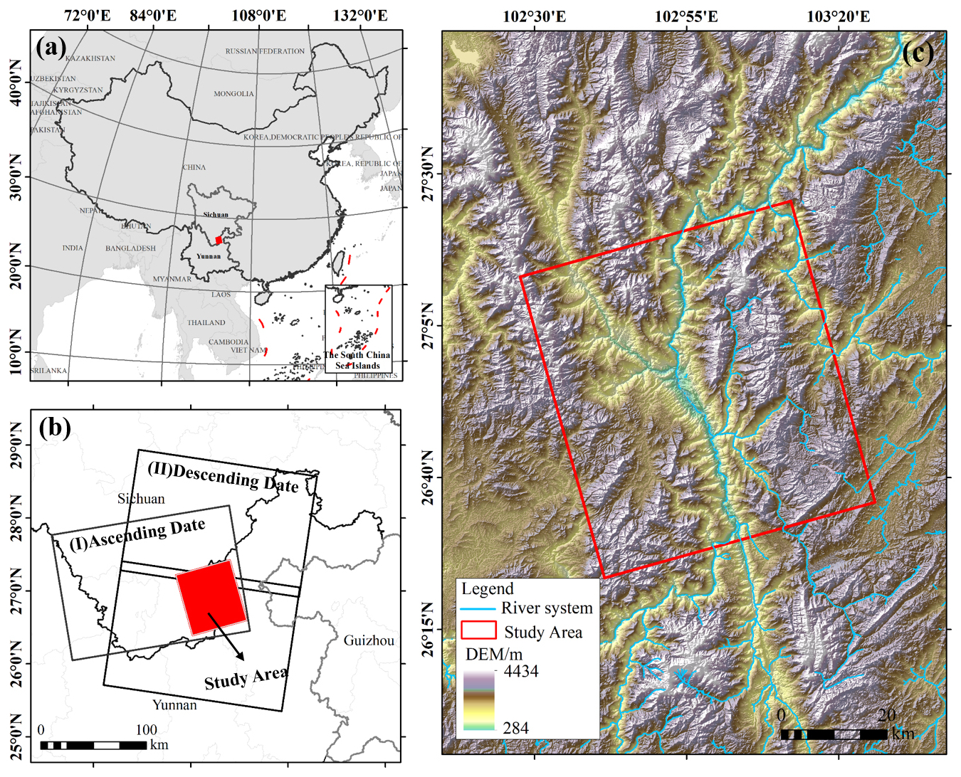
Figure 1 Overview of the Study Area.

The climate of the area is classified as a subtropical plateau monsoon climate, characterized by distinct wet and dry seasons, with an average annual precipitation of 822.7 mm. Precipitation is predominantly concentrated in the wet season, while the dry season is relatively arid. Due to the unique climatic conditions and abundant water resources, the stratigraphy of the reservoir area is complex, spanning multiple geological periods, including the Quaternary, Permian, and Carboniferous, with predominant rock types such as gravelly mixed soil, basalt, limestone, and sandstone (Yang, 2021) (Fig. 1b). The region is extensively covered by weak rock formations and loose materials, and the area has undergone multiple tectonic movements, leading to fractured and jointed bedrock. Active fault zones, such as the Zemuhe and Xiaojiang fault zones, are also present in the region (Dun et al., 2023) (Fig. 1c), with a predominantly north-south orientation and left-lateral strike-slip motion. After the reservoir impoundment, fluctuations in water levels, prolonged immersion of the slopes by reservoir water, and seasonal dry-wet cycles contribute to the formation of a high-risk environment for geological hazards, including landslides, collapses, and debris flows.

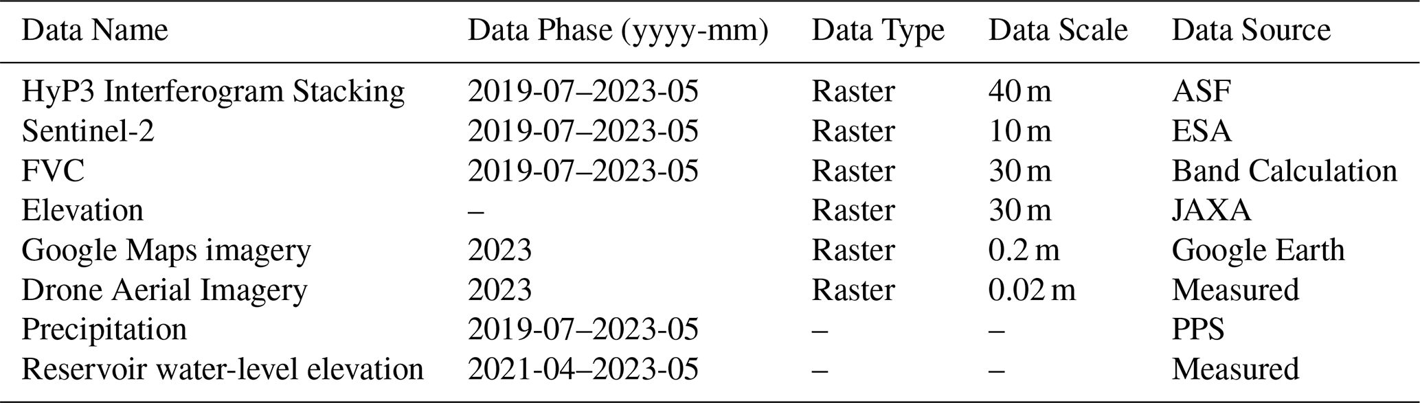
2.2 Research Data

2.2.1 HyP3 InSAR Data

This study uses the HyP3 interferometric data stack, produced by the Alaska Satellite Facility (ASF) cloud platform, as the experimental dataset for interferometric baseline optimization and atmospheric error correction. The data can be accessed and freely applied for online retrieval through the ASF website (https://search.asf.alaska.edu/#/, last access: 12 February 2024), with the application submitted on 18 May 2023. HyP3 is primarily used for processing Sentinel-1 data provided freely by the European Space Agency (ESA). Based on the ASF data platform, users can retrieve and query the Sentinel-1 SAR data archive. The main interferometric products available include wrapped and unwrapped interferograms, coherence maps, amplitude images, water mask images, DEMs, and look vector maps, etc. HyP3 utilizes Amazon's infrastructure services, including Amazon Elastic Compute Cloud (EC2) and Amazon Simple Storage Service (S3). It provides users with customized, on-demand synthetic aperture radar (SAR) processing services, eliminating the need for users to purchase or install complex SAR processing software and acquire advanced SAR processing skills. After the user submits an application through the ASF Vertex website or using the HyP3 Python SDK, the system automatically processes the interferometric data using GAMMA software hosted by Amazon Web Services (AWS). The process uses the Copernicus GLO-30 DEM to remove terrain phases and applies the minimum cost flow (MCF) method for phase unwrapping, ultimately generating interferometric products suitable for coherence analysis and with moderate pixel spacing. HyP3 data effectively addresses the issues associated with traditional interferometric processing methods, which require significant disk space, computational resources, and processing time, offering a new approach for large-scale reservoir bank landslide detection and monitoring.

The HyP3 platform supports customizable temporal and spatial baseline settings. Considering the monthly variation in vegetation coverage in deep-cut mountain canyon areas, and to avoid phase unwrapping issues and the introduction of additional errors, this study sets the temporal baseline threshold to 36 days. Notably, the Sentinel-1 satellite has a relatively short revisit cycle, and it revisits the same location multiple times over short spatial distances, making the impact on coherence negligible. Therefore, no spatial baseline threshold is set. Long-term interferograms from July 2019 to May 2023 were obtained using the baseline tool provided by the HyP3 online service platform (Fig. S1 in the Supplement).

2.2.2 Auxiliary Datasets

The auxiliary datasets used in this study include several key sources. Sentinel-2 data (Level 2A) with a 10 m spatial resolution, including red, blue, and green bands, was utilized to refine the estimation of surface vegetation coverage (Fraction of Vegetation Coverage, FVC) in the study area. This data was accessed online from Copernicus (https://dataspace.copernicus.eu/, last access: 20 August 2024). Additionally a 30 m resolution Digital Elevation Model (DEM) from the ALOS WORLD 3D dataset, provided by the Japan Aerospace Exploration Agency (JAXA), was used to calculate topographic features like mountain shadow, slope, aspect, and curvature. This dataset was accessed from ALOS (https://search.asf.alaska.edu/#/, last access: 1 July 2024). High-resolution Google Earth imagery with a 0.2 m spatial resolution was employed for location annotation of reservoir-bank landslides and for overlaying the acquired InSAR deformation results. This data was accessed from Google Earth (https://earthengine.google.com/, last access: 18 July 2024). Drone aerial imagery with a 0.1 m resolution was also used for field surveys to validate landslide identification results and to observe the Optical Characteristics of typical reservoir-bank landslides, with the imaging conducted on 14 May 2023. Precipitation data, acquired from the precipitation processing system on 15 July 2023, were used to analyze rainfall patterns, and Reservoir water-level elevation data were measured in the field during the research period. These datasets, summarized in Table 1, provided comprehensive support for the research.

Table 1 Data sources and specifications.

3 Research Methods and Data Processing

The main technical process of this study is as follows Fig. 2: (1) calculation of vegetation coverage and classification of interferogram stacks; (2) interferometric baseline optimization and atmospheric error correction; (3) surface deformation information acquisition and reservoir bank landslide identification and monitoring.

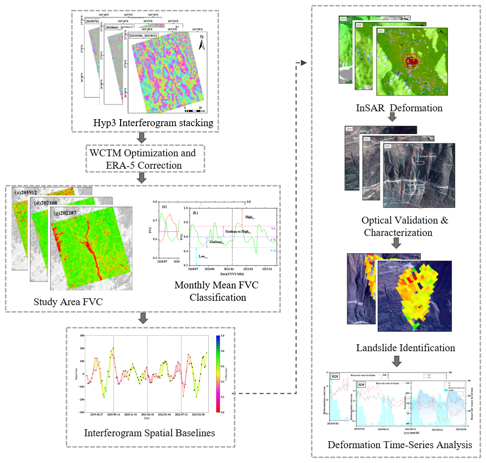
Figure 2 The technical flowchart of this study.

3.1 Vegetation Coverage Calculation Based on the Pixel Dichotomy Method

This study utilizes Sentinel-2 optical imagery from July 2019 to May 2023 and employs the Band Math tool to calculate the Normalized Difference Vegetation Index (NDVI) across the study area. To minimize the influence of non-landslide-related surface features, NDVI values were processed based on the pixel dichotomy model (Pi et al., 2021) to derive the Fractional Vegetation Cover (FVC) on a monthly scale (Fig. S2, as expressed in Eq. (3) presents the spatial and temporal variations in FVC, clearly reflecting seasonal vegetation dynamics – higher vegetation coverage is observed in summer months (e.g., August 2020 and July 2022), while markedly lower values appear during winter periods (e.g., December 2019 and December 2022). These seasonal changes in vegetation coverage significantly impact interferometric coherence and phase unwrapping performance in SBAS-InSAR processing. The vegetation temporal patterns revealed in FVC maps serve as a critical foundation for the development of the proposed Vegetation-Adaptive WCTM, enabling dynamic adjustment of coherence thresholds to mitigate decorrelation effects associated with vegetation growth cycles in deeply incised mountainous canyon environments.

$$\begin{array}{}\text{(1)}& \begin{array}{rl}& \mathrm{FVC}=\\ & \left\{\begin{array}{ll}\mathrm{0},& \mathrm{NDVI}\le {\mathrm{NDVI}}_{\mathrm{soil}}\\ \frac{\mathrm{NDVI}-{\mathrm{NDVI}}_{\mathrm{soil}}}{{\mathrm{NDVI}}_{\mathrm{veg}}-{\mathrm{NDVI}}_{\mathrm{soil}}},& {\mathrm{NDVI}}_{\mathrm{soil}}\le \mathrm{NDVI}\le {\mathrm{NDVI}}_{\mathrm{veg}}\\ \mathrm{1},& \mathrm{NDVI}\ge {\mathrm{NDVI}}_{\mathrm{veg}}\end{array}\right.\end{array}\end{array}$$

In the equation, FVC represents the monthly average vegetation coverage, NDVI represents the total value of the vegetation index for the pixel, NDVI_soil represents the NDVI value of pixels with no vegetation coverage, and NDVI_veg represents the NDVI value of pixels fully covered by vegetation.

3.2 WCTM Optimization of Interferometric Baseline

The WCTM considers the monthly variation of vegetation coverage in the time series and divides the interferogram into different coherence segments based on the vegetation coverage levels. The number of interferograms in each coherence segment is calculated, and the coherence coefficient is assigned a weight according to the number of interferograms in each segment. The final coherence coefficient optimization threshold is determined using a weighted averaging model. The process of optimizing the interferometric baseline using WCTM is as follows:

1. Calculate the point coherence and average coherence for each interferogram. Coherence is an important indicator for describing the quality of the interferometric phase. It is defined by the cross-correlation function during the registration of two complex images. The coherence at a pixel point (i,j) in the interferogram is defined as:

   $$\begin{array}{}\text{(2)}& r_{\left(i,j\right)}={\displaystyle \frac{\left|\sum _{i=\mathrm{1}}^m\sum _{j=\mathrm{1}}^{n}M\left(i,j\right)S^{\ast }\left(i,j\right)\right|}{\sqrt{\sum _{i=\mathrm{1}}^m\sum _{j=\mathrm{1}}^n{\left|M\left(i,j\right)\right|}^{\mathrm{2}}\sum _{i=\mathrm{1}}^m\sum _{j=\mathrm{1}}^n{\left|S\left(i,j\right)\right|}^{\mathrm{2}}}}}\end{array}$$

   In the formula, (i,j) represents the pixel coordinates of the interferogram at a certain point in the radar slant range coordinates, m and n represent the local window sizes for coherence calculation, and M and S represent the acquisition of two different Synthetic Aperture Radar (SAR) data. ∗ represents the complex conjugate of a given complex number.

   After calculating the pixel coherence point by point, the coherence for each interferogram in the study area can be calculated using Eq. (3):

   $$\begin{array}{}\text{(3)}& r_{\mathrm{avg}}={\displaystyle \frac{\sum _{i=\mathrm{1}}^P\sum _{j=\mathrm{1}}^Q{r}_{\left(i,j\right)}}{P\times Q}}\end{array}$$

   In the formula, (i,j) represents the coherence coefficient of each interferogram, with a value range from 0 to 1. (i,j) denotes the pixel coordinates of the interferogram at a specific point in radar slant-range coordinates. r_(i,j) represents the coherence at the pixel point (i,j), and P and Q represent the length and width of the interferogram image, respectively.

2. Classify the vegetation coverage levels of the time series.

3. Divide the interferograms into different coherence segments.

4. Assign weights to the coherence coefficients and use the weighted average model to optimize the coherence coefficient threshold. Calculate the number of interferograms under different vegetation coverage levels, assign weights to each coherence segment, and calculate the optimized interferometric baseline threshold based on the weights of different coherence segments:

   $$\begin{array}{}\text{(4)}& r_{\mathrm{WCTM}}=\sum _{i=\mathrm{1}}^I{\displaystyle \frac{m_i{r}_i}{n}}\end{array}$$

   In the equation, r_WCTM represents the optimized interferometric baseline threshold using the WCTM method, I represents the total number of coherence segments, m_i represents the number of interferograms in each coherence segment, r_i represents the average coherence of the interferograms in each coherence segment, n represents the total number of interferograms generated from all SAR acquisitions during the study period.

3.3 Correction of Atmospheric Delay Errors Using ECMWF ERA-5 Products

SAR signals are influenced by changes in atmospheric pressure, temperature, and humidity during propagation, leading to tropospheric delay effects (Li et al., 2023; Yang et al., 2023). The fifth-generation meteorological reanalysis dataset provided by European Centre for Medium-Range Weather Forecasts (ECMWF) offers high temporal resolution (hourly) and high spatial resolution (0.1), providing numerical weather model data on temperature, humidity, and pressure across 37 atmospheric pressure levels. This information can be effectively used to calculate atmospheric hydrostatic delay and correct atmospheric delay errors (Mandal et al., 2021; Soares et al., 2020).

$$\begin{array}{}\text{(5)}& N={\left(k_{\mathrm{1}}{\displaystyle \frac{P}{T}}\right)}_{\mathrm{hydro}}+{\left(k^{\prime }{\displaystyle \frac{e}{T}}+k_{\mathrm{3}}{\displaystyle \frac{e}{T^{\mathrm{2}}}}\right)}_{\mathrm{wet}}=N_{\mathrm{hydro}}+N_{\mathrm{wet}}\end{array}$$

In the equation, N_hydro represents the fluid static refractive component of the atmospheric refractive index, N_wet represents the wet refractive component of the atmospheric refractive index, P is the total atmospheric pressure, T is the temperature in Kelvin, e is the water vapor pressure, and k is the empirical constant. At this point, the integral value of the refractive index between the tropospheric zenith direction h_top and the height along the radar line of sight h is:

$$\begin{array}{}\text{(6)}& {\mathit{\phi }}_{\mathrm{tropo}}=-{\displaystyle \frac{\mathrm{4}\mathit{\pi }}{\mathit{\lambda }}}\cdot {\displaystyle \frac{{\mathrm{10}}^{-\mathrm{6}}}{\cos \mathit{\theta }}}\underset{h}{\overset{h_{\mathrm{top}}}{\int }}\left(N_{\mathrm{hydro}}+N_{\mathrm{wet}}\right)\mathrm{d}h\end{array}$$

In the equation, φ_tropo represents the bidirectional tropospheric delay phase, λ denotes the radar center wavelength, and θ is the satellite incidence angle.

For InSAR measurements, the tropospheric delay phase in the interferogram is the difference in tropospheric delay between the imaging points of the master and secondary images. Due to slight differences in atmospheric conditions between the two acquisitions, the tropospheric delay error for two imaging points (q,p) at times m and n can be expressed as:

$$\begin{array}{}\text{(7)}& \begin{array}{rl}\mathrm{\Delta }{\mathit{\phi }}_{\mathrm{tropo}}\left[\left(p,q\right),\left(t_m,t_n\right)\right]& =\left[{\mathit{\phi }}_{\mathrm{tropo}}\left(p,t_n\right)-{\mathit{\phi }}_{\mathrm{tropo}}\left(p,t_m\right)\right]\\ & -\left[{\mathit{\phi }}_{\mathrm{tropo}}\left(q,t_n\right)-{\mathit{\phi }}_{\mathrm{tropo}}\left(q,t_m\right)\right]\end{array}\end{array}$$

3.4 SBAS-InSAR Processing

SBAS-InSAR technology efficiently synthesizes all available small baseline interferograms, selects coherent target points for modeling and calculation, and removes atmospheric delays via temporal filtering to obtain high spatial density surface deformation results (Fan et al., 2016; Zhang et al., 2012). In this study, we use the open-source software package Mintpy (The Miami InSAR Timeseries Software in Python) for SBAS-InSAR processing (Zhang et al., 2019). We load the selected ascending track interferogram stack from July 2019 to May 2023 into the Mintpy software. A reference pixel with high coherence (we set the threshold) is chosen from a region far from the deformation area. Then, the initial phase value θ_n and estimated phase value φ_n are used to evaluate the quality of each pixel in the raw phase time series, as shown in Eq. (8):

$$\begin{array}{}\text{(8)}& r={\displaystyle \frac{\mathrm{1}}{N^{\mathrm{2}}-N}}\sum _{n=\mathrm{1}}^N\sum _{k\ne n}^N{e}^{i{\mathit{\theta }}_{nk}}{e}^{-i\left({\mathit{\phi }}_n-{\mathit{\phi }}_k\right)}\end{array}$$

In the equation, N represents the number of SAR images, i refers to a single SAR image, and n and k represent the wrapped phase interferograms collected at corresponding times. To ensure data quality and the accuracy of InSAR measurements, the root mean square error (RMSE) of the residual phase is used to estimate the noise present in the time series:

$$\begin{array}{}\text{(9)}& {\mathrm{RMSE}}_i=\sqrt{{\displaystyle \frac{\mathrm{1}}{N_{\mathrm{\Omega }}}}{\sum }_{P\in \mathrm{\Omega }}{\left(-{\widehat{\mathit{\phi }}}_{\mathrm{resid}}^i\left(p\right)\cdot {\displaystyle \frac{\mathit{\lambda }}{\mathrm{4}\mathit{\pi }}}\right)}^{\mathrm{2}}}\end{array}$$

In the equation, $i=[\mathrm{1},\mathrm{\dots },N]$ and Ω represent reliable pixels selected from the temporal coherence mask, λ is the radar center wavelength, and ${\widehat{\mathit{\phi }}}_{\mathrm{resid}}^i$ represents the redundant phase at time i. After applying the noise mask, the average deformation rate in the study area is estimated from the time series using Eq. (10):

$$\begin{array}{}\text{(10)}& v_{\mathrm{los}}\cdot t_i+c=-{\widehat{\mathit{\phi }}}_{\mathrm{disp}}^i\cdot {\displaystyle \frac{\mathit{\lambda }}{\mathrm{4}\mathit{\pi }}}\end{array}$$

In the equation, v_los represents the average deformation rate in the radar line-of-sight direction, t_i denotes the time of SAR acquisition at time i, c is the unknown deformation offset constant, and ${\widehat{\mathit{\phi }}}_{\mathrm{disp}}^i$ represents the displacement time series.

4 Results and Analysis

4.1 Results of Interference Baseline Optimization Using WCTM

Based on the 345 HyP3 interferograms from July 2019 to May 2023, with 3 July 2019, as the reference image date, the baseline connection map for all interferograms was obtained (Fig. 3). It can be observed that the average coherence coefficient in the Baihetan Reservoir area exhibits distinct seasonal variation, specifically with higher average coherence during the winter and lower average coherence during the summer. This pattern aligns with seasonal changes in vegetation and the regional dry-wet climate cycle.

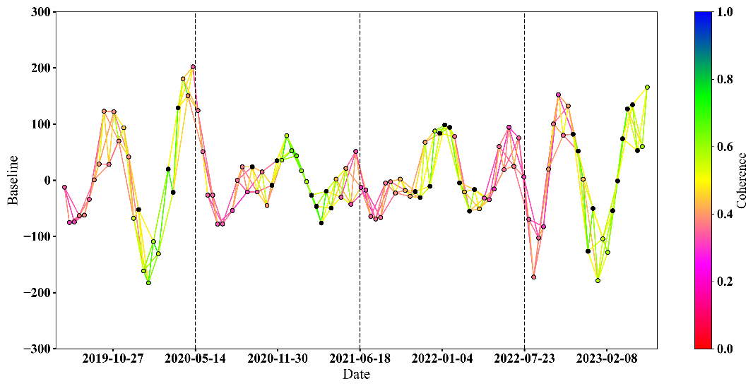
Figure 3 Spatio-Temporal Baseline Network of All Interferograms (the red dashed line represents a spatial baseline value of 0, the black dashed lines indicate December 31 of each year, and the red-to-blue gradient represents the average coherence of each interferogram).

To further explore the relationship between the average coherence coefficient and vegetation coverage in the Baihetan Reservoir area, monthly average vegetation coverage was calculated based on the pixel binary model (Eq. 1), and a time series curve was established between the monthly average coherence of the interferograms and the vegetation coverage (Fig. 4a). The variation in the average coherence coefficient in the study area shows a significant correlation with changes in vegetation coverage. The WCTM method proposed in this study was used to optimize the interferometric baseline threshold. Based on the objective distribution characteristics of the FVC data and with reference to classification criteria used in similar regions, this study establishes a vegetation-based categorization scheme. Accordingly, the monthly average vegetation coverage in the study area was classified into four levels (Li et al., 2004): low vegetation coverage (< 45 %), medium vegetation coverage (45 %–60 %), medium-high vegetation coverage (60 %–75 %), and high vegetation coverage (> 75 %). Based on the classified vegetation coverage levels, the monthly average coherence coefficient was divided into four coherence segments (Fig. 5b). These segments accounted for 2.1 %, 57.5 %, 23.4 %, and 17.0 % of the total interferograms, respectively. These proportions were used as weights to calculate the optimized interferometric baseline threshold (λ_WCTM=0.4882) using the WCTM method. Interferograms with average coherence coefficients below this threshold were excluded, and the remaining 146 optimized interferograms were retained for SBAS-InSAR processing.

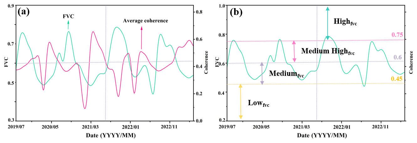
Figure 4 Monthly Average Vegetation Coverage Time Series. Panel (a) shows the relationship between monthly average vegetation coverage and monthly average coherence coefficient; panel (b) presents the classification results of monthly average vegetation coverage levels. The black dashed line represents the midpoint date of the study period.

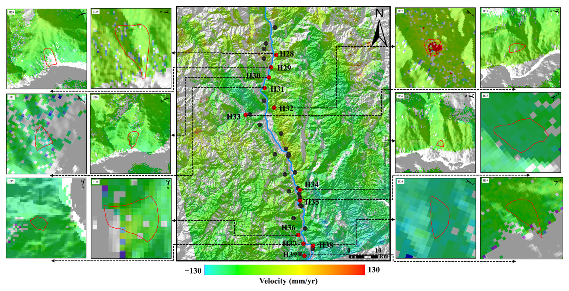
Figure 5 Localized InSAR deformation signals for the early identification of reservoir-bank landslides. Note: The red polygons represent the geological boundaries of historical landslides delineated based on geomorphic features such as rear scarps and frontal bulging; the InSAR monitoring results characterize the current surface deformation during the study period. The reasons for the discrepancy between them are as follows: (1) the deformation rate of some landslides is below the detection limit of InSAR; (2) severe decorrelation (coherence < 0.2) caused by slope vegetation cover interferes with deformation signal extraction; (3) radar geometric distortion induced by steep terrain impairs signal monitoring effectiveness.

Due to the inherent limitations of C-band radar wavelength, coherence significantly deteriorates in areas with vegetation coverage exceeding 75 % (particularly during summer, as shown in Fig. 4a). This results in the omission of small-scale landslides within steep canyon slopes (> 45° inclination). Analysis using 30 m-resolution ALOS DEM data indicates such terrain accounts for approximately 12.7 % of the total study area. Future investigations could enhance detection capabilities through integration with L-band SAR data.

4.2 Early Detection Results of Reservoir-bank landslides

The SBAS-InSAR processing was performed on the HyP3 interferometric stack optimized using the WCTM method with the open-source software MintPy 1.5.1. Additionally atmospheric delay errors in the interferometric stack were corrected using the ECMWF ERA-5 product. As a result, radar line-of-sight surface deformation information from July 2019 to May 2023 was successfully obtained. Positive deformation values indicate motion towards the sensor, while negative values indicate motion away from the sensor. The absolute value of the deformation rate represents the magnitude of the deformation rate.

Based on relevant literature and the complex geological conditions in the Baihetan Reservoir area, C-band SAR data can be used to monitor slope deformation. In this region, if the annual deformation rate of a slope exceeds 16 mm yr⁻¹, it is considered to indicate potential landslide hazards. In this study, considering factors such as resettlement activities, frequent human activities, and deformation signal errors within the reservoir area, a threshold of 16 mm yr⁻¹ was set for identifying potential reservoir-bank landslides. Specifically, when the deformation rate of a slope exceeds 16 mm yr⁻¹, it is considered a suspected landslide area. To further assess landslide risks, this study combined SAR deformation signals with the established threshold to initially delineate suspected landslide areas. Additionally high-resolution optical images (e.g., Google Earth imagery) were used to conduct a detailed analysis of features such as color, structure, topographic morphology, landslide boundaries, and cracks for early detection and localization of reservoir-bank landslides (Fig. 5).

A total of 39 potential reservoir-bank landslides were identified in the Baihetan Reservoir area Among the early identified landslides, 27 were historical landslide hazards, numbered H1-H27; 12 new landslides were identified, numbered H28–H39. The interpretation of the remote sensing images is shown in Fig. 6.

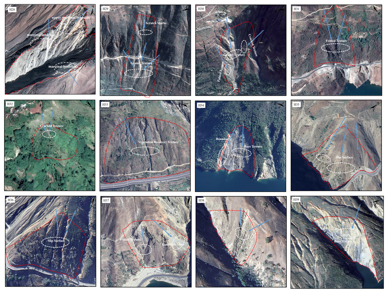
Figure 6 Optical characteristics of representative reservoir-bank landslides based on Google Earth imagery (Imagery © 2025 Landsat/Copernicus, Map data © 2025 Google).

4.3 Analysis of Typical Reservoir Bank Landslide Deformation Trend Evolution

Based on the early identification results of reservoir-bank landslides presented in Sect. 4.2, the H28 and H30 landslides were selected from the Baihetan Reservoir catchment for detailed analysis of their deformation evolution characteristics using Google Earth imagery. High-resolution images clearly reveal typical landslide features, including cracks, frontal bulging, subsidence, and slope fragmentation.

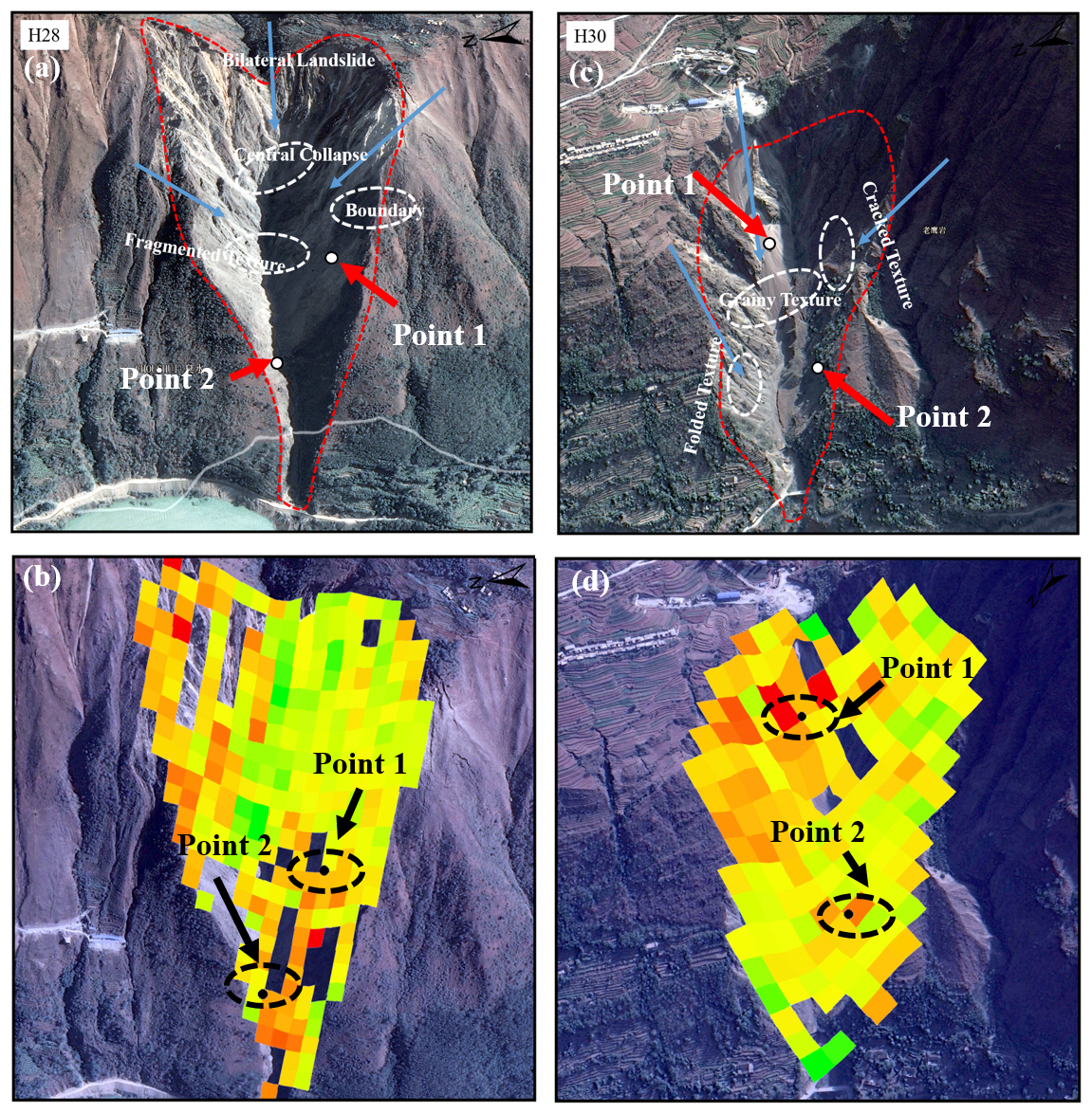
Figure 7 Remote sensing interpretation of typical reservoir-bank landslides based on optical features derived from Google Earth imagery and corresponding InSAR deformation signals (Imagery © 2025 Landsat/Copernicus, Map data © 2025 Google).

The H28 landslide, situated in Miansha Village, Qiaojia County on the eastern bank of the upper Jinsha River reservoir section, demonstrates two distinct deformation zones in the InSAR deformation signals (Fig. 7b) – one along the right slip surface and another at the slope toe. Google Earth imagery interpretation indicates bilateral sliding toward the center, forming an irregularly shaped “bidirectional landslide” characterized by a wider upper section and narrower lower extent. The steep slope exhibits significant surface subsidence with rough textures (Fig. 7a), while granular accumulations are visible in the basal trough. More pronounced displacement traces on the right slope compared to the left suggest the landslide is likely in a state of prolonged sliding activity.

Located on the western bank of the lower Baihetan Reservoir area in Shuicaozi Village, Huidong County, the H30 landslide displays a tongue-shaped irregular boundary with prominent concave morphology. The slope deformation manifests primarily as compressional displacement from both sides toward the center (Fig. 7c), with greater deformation intensity observed on the right slip surface. Fractures and debris deposits identified in the central portion of the landslide body, coupled with pronounced deformation zones at the upper-left and lower-right sections (Fig. 7d), further confirm its active deformation state.

Figure 8 Time Series Deformation Curves of Typical Landslide Feature Points.

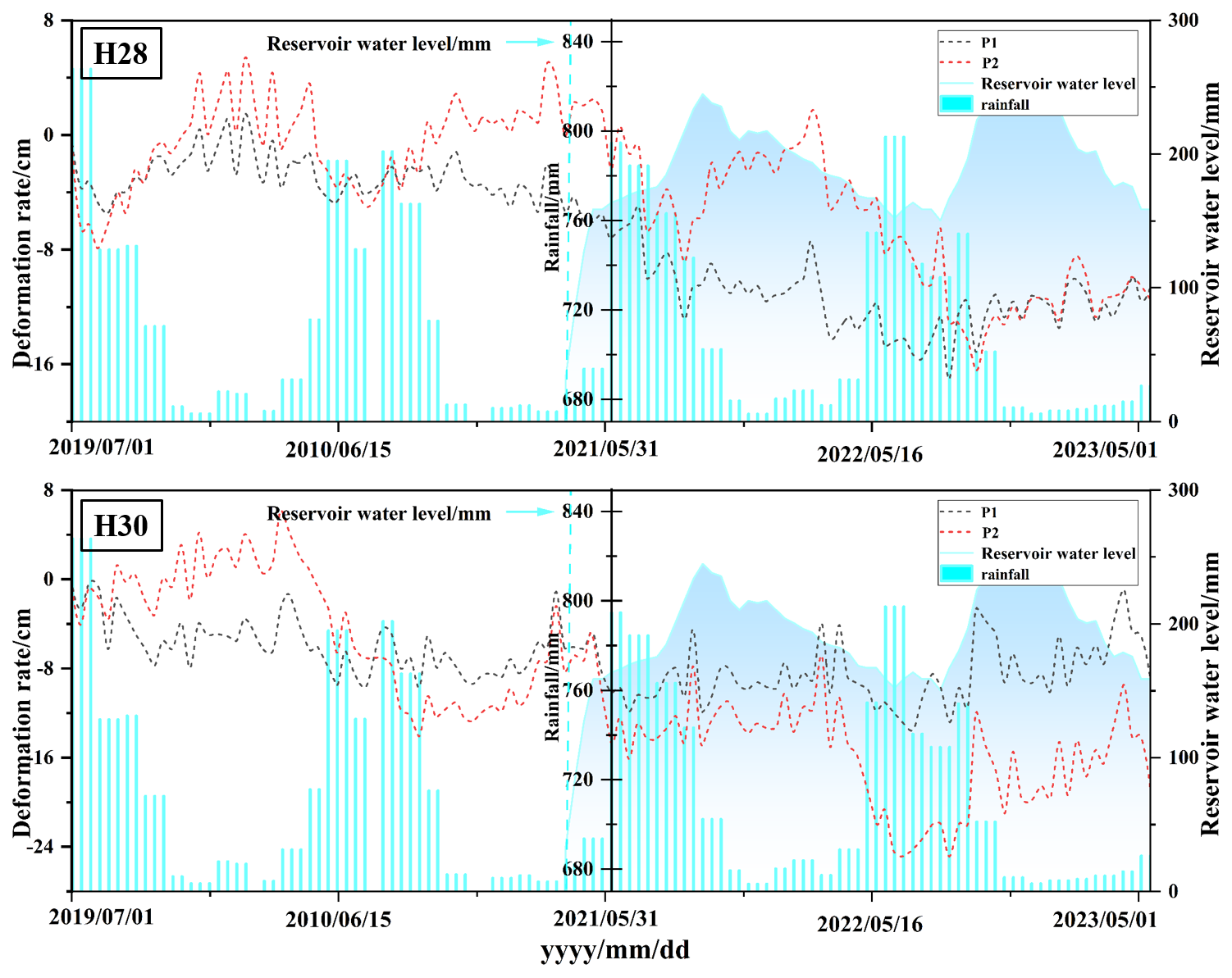
This study analyzed the temporal evolution characteristics of reservoir-bank landslide deformation. Characteristic points with significant deformation (H28 P1, H28 P2, H30 P1, and H30 P2) were selected from the H28 and H30 landslide areas in the Baihetan Reservoir, and time-series deformation curves were constructed (Fig. 8).

As observed from the time-series deformation curves, the deformation of characteristic points is not synchronized with reservoir water level variations, exhibiting an obvious time-lag effect. To accurately quantify this lag relationship, this study employs the signal cross-correlation analysis method, with the core calculation formulas presented as follows:

1. Cross-Correlation Coefficient Calculation Formula

   $$\begin{array}{}\text{(11)}& R_{xy}\left(\mathit{\tau }\right)={\displaystyle \frac{E\left[(X_t-{\mathit{\mu }}_X)(Y_{t+\mathit{\tau }}-{\mathit{\mu }}_Y)\right]}{{\mathit{\sigma }}_X{\mathit{\sigma }}_Y}}\end{array}$$

   Where: R_xy(τ) is the cross-correlation coefficient corresponding to the lag step τ; R_xy(τ) is the landslide deformation observation value at time t; Y_t+τ is the reservoir water level observation value at time t+τ; μ_X and μ_Y are the means of the deformation sequence and water level sequence, respectively; σ_X and σ_Y are the standard deviations of the two sequences, respectively; E[⋅] denotes the mathematical expectation operator.

2. Optimal Lag Time Determination Formula

   $${\mathit{\tau }}_{\mathrm{opt}}=\underset{\mathit{\tau }\in [-{\mathit{\tau }}_{max},{\mathit{\tau }}_{max}]}{\mathrm{argmax}}\left|R_{xy}\right(\mathit{\tau }\left)\right|$$

   where τ_opt is the optimal lag time (a negative value indicates that deformation precedes water level changes); argmax is the operator that takes the independent variable corresponding to the maximum value; τ_max is the preset maximum lag step (100 steps in this study).

In the H28 landslide, P1 is located in the upper-middle part of the landslide, while P2 is situated in the lower part. Both points exhibit deformation moving away from the satellite along the radar line of sight. Precipitation and reservoir water level variations at the Baihetan Reservoir are identified as the primary controlling factors for landslide deformation. During the 2021 impoundment period, when the water level reached the maximum elevation of 816.5 m, the cumulative deformation of both characteristic points before and after impoundment exceeded 10 centimeters, indicating a strong response of the H28 landslide to reservoir water level changes. After the completion of phased impoundment, P2 in the lower part showed a more stable deformation trend, which is inferred to stem from slope structure compaction and reduced looseness induced by rising water levels.

Throughout the two impoundment cycles, the deformation of P1 and P2 was asynchronous with water level fluctuations. The time-lag effect was quantified via signal cross-correlation analysis (Fig. 9). For H28 P1, the maximum correlation between deformation and reservoir water level corresponded to a lag time of −40 steps, meaning deformation preceded water level changes by 40 time units. For H28 P2, the maximum correlation lag time was −50 steps. Both correlation coefficients exceeded the statistical significance threshold, confirming the statistical significance of the time-lag effect.

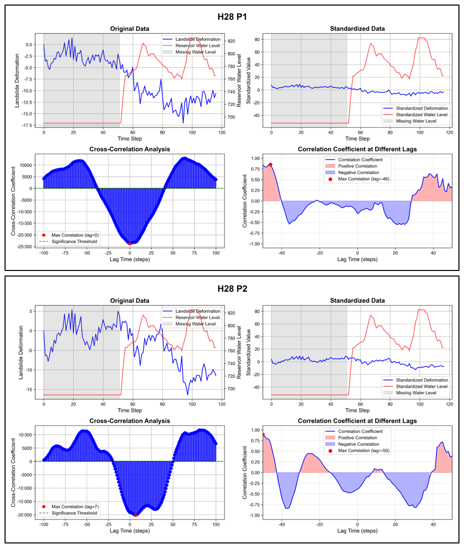
Figure 9 Analysis of Time-Lag Effect Between Deformation and Water Level for Characteristic Points of the H28 Landslide.

For the H30 landslide, P1 is located at the middle elevation of the left sliding surface, and P2 at the lower elevation of the right sliding surface. Both points exhibited deformation trends away from the satellite before and after impoundment. Compared with P2, P1 displayed a more stable deformation trend, implying the H30 landslide may possess rotational sliding characteristics, with sliding directions varying by elevation. During the 2021–2022 impoundment periods, the deformation peaks of P1 and P2 did not coincide with the water level peaks of 816.5 and 825 m. Further quantification through cross-correlation analysis (Fig. 10) revealed that the maximum correlation lag time for H30 P1 was −42 steps and −22 steps for H30 P2. Both results passed the significance test, further verifying the time-lag response of the landslide to water level variations. After the conclusion of impoundment, the cumulative deformation of P2 exceeded 10 centimeters, suggesting that water level changes may intensify landslide activity in this region.

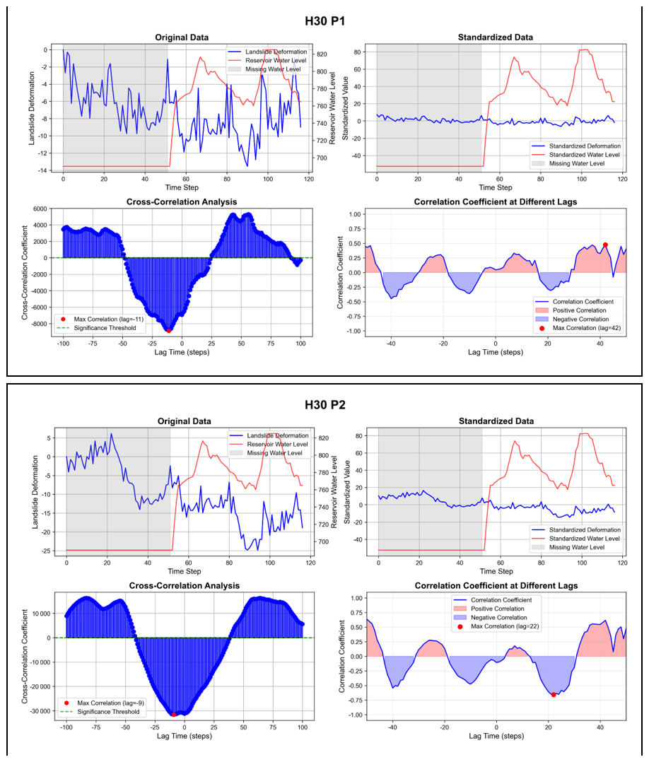
Figure 10 Analysis of Time-Lag Effect Between Deformation and Water Level for Characteristic Points of the H30 Landslide.

In summary, reservoir-bank landslide deformation is significantly affected by water level variations. Signal cross-correlation analysis enables clear quantification of this time-lag effect: the lag steps for characteristic points in the H28 area range from 40 to 50 steps, while those in the H30 area range from 22 to 42 steps. These quantified results provide data support for understanding the temporal response patterns of landslide deformation. Furthermore, they emphasize the importance of real-time monitoring and dynamic updates of reservoir-bank landslides for regional geological hazard prevention and mitigation.

5 Discussion and Conclusion

5.1 Discussion

5.1.1 Baseline Optimization Performance Evaluation

The WCTM method proposed in this paper takes into account the relationship between the InSAR coherence and the monthly variation in vegetation cover, which represents a specific improvement over previous studies. By comparing the WCTM method with traditional interference baseline selection methods (short time-space baseline threshold and average coherence threshold), the performance of the optimized interferometric baseline is evaluated through the calculation of deformation rate standard deviation (Figs. 11 and 12) and the full-phase ambiguity of the loop closure error (Fig. 13). As shown in Fig. 10, the deformation rate standard deviation with the short time-space baseline threshold (time baseline threshold: 36d, space baseline threshold: 200 m) exhibits an irregular and uneven spatial distribution along the Jinsha River (from south to north), with maximum and minimum deformation rate standard deviations observed in the northern and southern parts of the study area, respectively (Fig. 11a). This indicates that the short time-space baseline threshold is prone to introducing decorrelation errors, making it ineffective for obtaining stable InSAR deformation signals. The use of the average coherence threshold effectively improves the overall Stability of the InSAR signals, but some anomalies were still observed outside the reservoir banks of the Baihetan Reservoir (Fig. 11b). This suggests that simply setting an average coherence threshold through basic statistical methods does not reflect the seasonal variation in coherence caused by interference, and is not suitable for InSAR deformation signal detection in deeply-cut mountain canyon areas. The WCTM method, which optimizes the interferometric baseline by considering the relationship between coherence and vegetation cover, reduces the redundancy of low-coherence interferograms, effectively improving overall coherence, and avoids the subjectivity caused by expert experience and simple statistical methods. The deformation rate standard deviation shows a more uniform and Stable distribution (Fig. 11c). Furthermore, the statistical analysis of the deformation rate standard deviation distribution (Fig. 12) also confirms this, with the average deformation rate standard deviations for the short time-space baseline method, average coherence threshold method, and WCTM method being 1.7865, 1.4587, and 1.2668, respectively, and with quartile medians of 1.6802, 1.3831, and 1.1667. This demonstrates that the WCTM method, which optimizes interferometric baseline thresholds significantly reduced the time-series noise contained in the InSAR deformation signals, resulting in more effective and stable deformation rates.

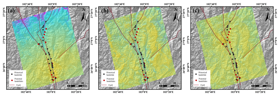
Figure 11 Standard Deviation of Deformation Rates: (a) results without interferometric baseline threshold optimization, (b) results with interferometric baseline optimization based on average coherence, (c) results with interferometric baseline optimization using the WCTM method.

Figure 12 Statistical Distribution of Deformation Rate Standard Deviation.

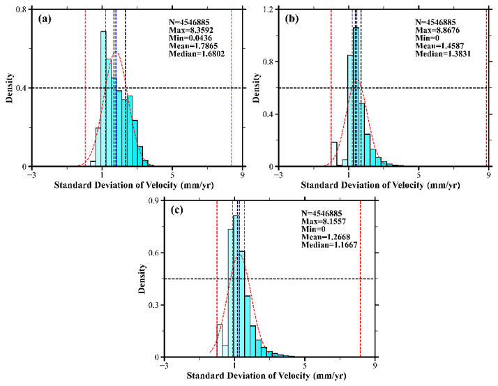
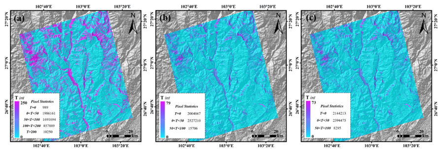
Figure 13 Integer Ambiguity of Circular Phase Closure Errors.

The WCTM method optimizes interferometric baseline thresholds, substantially reducing temporal noise in InSAR deformation signals, thereby yielding more reliable and stable deformation rate estimates. The relative reduction in the deformation rate standard deviation achieved by the WCTM method compared to the conventional short temporal baseline threshold method is quantitatively expressed as:

$$\begin{array}{}\text{(12)}& \mathrm{Reduction}={\displaystyle \frac{{\mathit{\sigma }}_{\mathrm{short}\mathrm{baseline}}-{\mathit{\sigma }}_{\mathrm{WCTM}}}{{\mathit{\sigma }}_{\mathrm{short}\mathrm{baseline}}}}\times \mathrm{100}\mathit{\%}\end{array}$$

Where σ_{short baseline} and σ_WCTM denote the mean deformation rate standard deviations obtained by the short temporal baseline threshold method and the proposed WCTM method, respectively. This result quantitatively demonstrates that the WCTM method reduces the deformation rate standard deviation by approximately 29.1 %, confirming its superior capability in improving the accuracy and stability of deformation measurements in complex mountainous canyon environments.

In addition, the full-phase ambiguity results of the loop phase closure check for phase unwrapping also validate the performance of the optimized interferometric baseline using the WCTM method proposed in this paper. The full-phase ambiguity of the loop closure describes the “periodicity” or “ambiguity” of radar phase during the phase unwrapping process in time-series InSAR technology, and is used to evaluate the quality of phase unwrapping and possible phase unwrapping errors. Figure 13 shows the full-phase ambiguity of the loop closure obtained using the three methods. It is not difficult to observe that, compared to the short time-space baseline threshold method, the optimization of interferometric baseline threshold using the coherence coefficient of the interferogram yields more robust phase unwrapping results, with a significant improvement in the quality of phase unwrapping. The non-zero values of the full-phase ambiguity of the loop closure are effectively reduced. By considering the monthly variation of InSAR coherence and vegetation cover, the WCTM method leads to an increase of 140 146 good unwrapping results (Tint = 0) compared to the average coherence threshold method, while the unwrapping errors with closure differences greater than 50 (50 times 2π) are reduced by 7411, indicating that the WCTM method effectively reduces the noise level detected by time-series InSAR technology and demonstrates good applicability in deeply-cut mountain canyon areas.

5.1.2 SBAS-InSAR Deformation Signal Accuracy Verification and Error Analysis

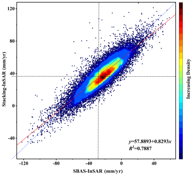
This paper describes a method for optimizing the interferometric baseline threshold of the HyP3 interferogram stack using the proposed WCTM method to obtain InSAR deformation signals for deeply incised high mountain canyon areas. The accuracy of the deformation signals is limited by the HyP3 interferogram stack products processed and released by the ASF. Due to the special terrain and topography of the Baihetan Reservoir area, the descending track data experiences significant geometric distortion. To improve the accuracy of the InSAR deformation signals and reduce the impact of geometric distortion on reservoir bank landslide identification results, we selected ascending track data from the HyP3 interferogram stack as the experimental dataset for the WCTM method. By comparing with historical landslide data from 2021, the spatial locations of the early-identified reservoir-bank landslides showed a high degree of similarity to the historical landslides, indirectly validating the accuracy of the InSAR results. However, due to the lack of GNSS observational data in the study area, we were unable to compare the detected InSAR deformation signals with GNSS data on a time-series scale. To quantitatively analyze the reliability of the InSAR results, we performed cross-validation by comparing deformation results obtained using different techniques on the same track. We used the HyP3 interferogram stack mentioned in Sect. 2.2 for Stacking-InSAR processing, obtaining the average phase velocity for the study period (Fig. 14b), and then performed a combined analysis with the deformation rates obtained using the SBAS-InSAR technique in Sect. 4.3. We randomly selected 25 141 deformation points from areas with consistent deformation trends (Fig. 14) for regression analysis (Fig. 15). The cross-validation results between SBAS-InSAR and Stacking-InSAR show an R² value of 0.79, which demonstrates that the surface deformation information obtained from both SBAS-InSAR and Stacking-InSAR methods is reliable on both temporal and spatial scales. Additionally, the cross-validation results also verify the accuracy and reliability of the time-series InSAR data optimized using the WCTM method proposed in this study.

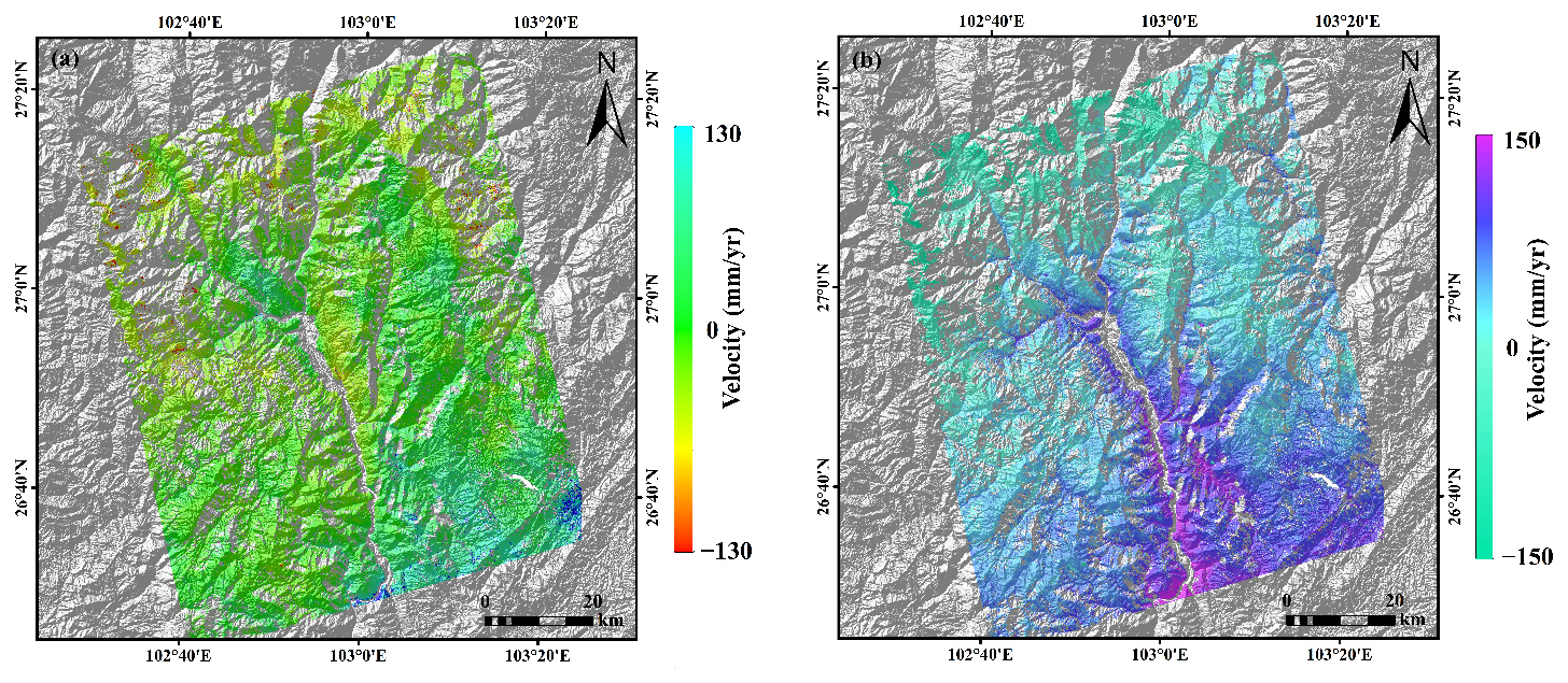
Figure 14 Deformation Information from SBAS-InSAR and Stacking-InSAR in the Study Area.

Figure 15 Cross-validation Results between Stacking-InSAR and SBAS-InSAR.

The SBAS-InSAR deformation inversion results are often affected by phase unwrapping errors and atmospheric delay errors. Optimizing these errors can significantly improve monitoring accuracy. The above experiments demonstrate that by adjusting the coherence threshold and optimizing the full-wavelength ambiguity of the phase closure, the WCTM method effectively improves the stability of phase unwrapping. Based on this, this study combined the ERA-5 meteorological reanalysis product released by the ECMWF to correct atmospheric delay errors, and compared the phase standard deviation of interferograms before and after correction (Fig. 16). The results show that after ERA-5 correction, the phase standard deviation significantly decreased, with the maximum phase standard deviation reduced from 11.81 to 5.27 rad. Notably, 71.2 % of the interferogram phase standard deviations showed significant improvement, while only 28.8 % of interferograms were negatively affected, with the maximum negative standard deviation being −4.48 rad. This indicates that the ERA-5 product, with its high spatiotemporal resolution, can effectively eliminate atmospheric delay errors in InSAR monitoring, and is particularly well-suited for deep-cut mountain canyon areas.

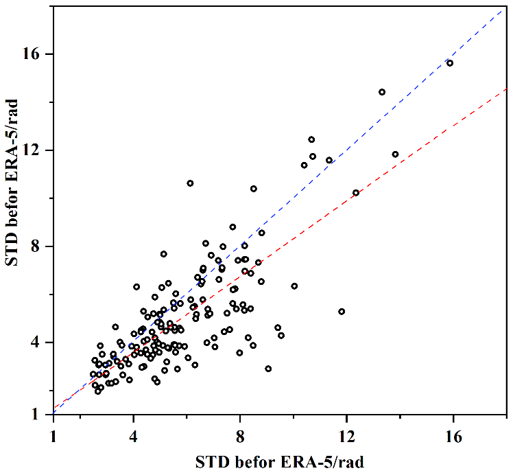
Figure 16 Correlation Analysis of Phase Standard Deviation Before and After ERA-5 Atmospheric Correction.

Figure 17 Statistical Chart of the Distribution Pattern of Reservoir-bank landslides.

5.1.3 Distribution Patterns of Reservoir-bank landslides and the Impact of Reservoir Water Level Changes on Landslide Deformation

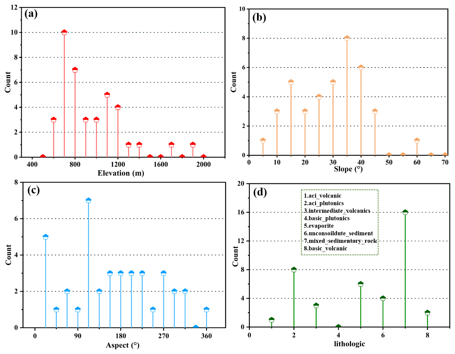
There are many factors that influence reservoir-bank landslides. Considering the geomorphological conditions of the Baihetan Reservoir, this study analyzes the distribution patterns of reservoir-bank landslides based on the 39 landslides identified in Sect. 4.2, using statistical methods and examining terrain factors such as elevation, slope, aspect, and lithology (Fig. 17). From Fig. 16, it can be seen that the identified reservoir-bank landslides are primarily concentrated within the elevation range of 600 to 1400 m and widely developed in slopes ranging from 30 to 45°. This indicates that slopes that are too gentle are not enough to induce slope movement, while steeper reservoir banks are more conducive to landslide development. The landslides identified in the early stages are mostly distributed in the northeast, east, and northwest directions, similar to the findings of Dun et al., with fewer landslides identified in the north-south direction. This could be due to the sensitivity of the Sentinel-1 satellite to deformation in the north-south direction being affected by its flight path. Additionally, the lithology of the reservoir-bank landslides mainly consists of mixed sedimentary rocks, carbonate rocks, and neutral volcanic rocks, which are generally located in incompetent strata. Previous studies suggest that the increase or decrease in pore water pressure on the sliding surface caused by changes in the reservoir water level is the primary factor triggering instability in reservoir-bank landslides. Moreover, under different reservoir water level change patterns, the deformation signals of the landslides show significant differences. Notably, in Sect. 4.3, the analysis of landslide deformation trend evolution indicates that the peak of landslide deformation does not coincide with the peak of the reservoir water level, suggesting a time-lag response of landslide deformation to the water level changes in the Baihetan Reservoir. This phenomenon is similar to previous research. The time-lag effect includes a time delay in the deformation process of the landslide and irreversible plastic deformation of the landslide's geological structure during the water level change process. As the pore water pressure in the landslide changes, it affects the stability of the slope. The stress state of the soil also needs time to adjust to and adapt to the new pressure conditions. Therefore, when the reservoir water level changes, the moisture within the landslide requires a certain period to reach a new equilibrium state, which is why the deformation of the reservoir-bank landslides shows a clear lag response to water level fluctuations.

In summary, the WCTM method proposed in this study demonstrates effectiveness in the early identification of reservoir landslides in deeply incised alpine gorge areas. The core advantage of this approach lies in its ability to resolve the decorrelation problem caused by seasonal vegetation changes – a challenge prevalent in numerous surface deformation monitoring scenarios. Consequently, the methodology can be extended to the following application scenarios: monitoring of other types of reservoir landslides, identification of geological hazards such as landslides and collapses in vegetated mountainous areas, and stability monitoring of engineering structures in regions with significant seasonal vegetation variations.

5.2 Conclusion

This study focused on the Baihetan Hydropower Station reservoir area, utilizing Sentinel-1A ascending and descending track data from July 2019 to May 2023. The Vegetation-Adaptive WCTM was employed to optimize interferometric baseline thresholds, combined with atmospheric delay correction using the ERA-5 meteorological reanalysis product. The main conclusions are as follows:

1. Compared with the traditional short temporal-spatial baseline threshold method and the average coherence threshold method, the WCTM approach achieved an average reduction of 0.520 and 0.192 in the SD of deformation signals, and median reductions of 0.514 and 0.216, respectively, significantly improving phase unwrapping quality. After atmospheric delay correction, 71.2 % of the interferograms exhibited a substantial decrease in phase SD, with the maximum phase SD was reduced from 11.81 to 5.27 rad. These results demonstrate the superiority of the proposed method in enhancing data quality.

2. Using the InSAR deformation signals optimized by the WCTM, early identification of reservoir-bank landslides in deeply incised mountainous canyon areas was successfully achieved, with a total of 39 landslides detected. Field validation via drone surveys confirmed the applicability and robustness of the method, and detailed analyses of the spatial distribution and temporal evolution of landslides were conducted.

3. Statistical analysis revealed that most reservoir-bank landslides in the Baihetan area occur within an elevation range of 600 to 1400 m and on slopes between 30 and 45°. The predominant slope aspects are northeast, east, and northwest. Lithologically, these landslides mainly develop on carbonate rocks, intermediate volcanic rocks, mixed sedimentary rocks, and siliceous clastic sedimentary rocks.

In summary, the WCTM method provides an effective technical means for high-precision monitoring of reservoir-bank landslides in complex mountainous regions, offering significant theoretical and practical value for regional landslide disaster prevention and mitigation.