Simulating spatial multi-hazards with generative deep learning

When natural hazards coincide or spread across large areas they can create major disasters. For accurate risk analysis, it is necessary to simulate many spatially resolved hazard events that capture the relationships between extreme variables, but this has proved challenging for conventional statistical methods, particularly in high-dimensional settings. In this article we show that generative deep learning models – when combined with specific transformations to the training data – offer a useful alternative method for stochastically sampling realistic multi-hazard events. Our framework combines generative adversarial networks with extreme value theory in a hybrid approach that can capture complex dependence structures in gridded multivariate weather data, while providing a theoretical basis for extrapolation to new extremes. We apply our method to jointly model fields of strong winds, heavy precipitation, and low atmospheric pressure (∼ 12 000 variables) during storms in the Bay of Bengal, demonstrating that our model learns the spatial and multivariate extremal dependence structures of the underlying data and captures the distribution of storm severities. For the Bay of Bengal case study, we validate our approach against a popular model for multivariate climate extremes, and demonstrate improved performance in capturing the extremal correlation structure.

1 Introduction

Hazards that entail several extreme weather variables and extend over large spatial domains are responsible for some of the most damaging natural catastrophes (Zscheischler et al., 2018). Compound hazards can be broadly grouped into four typologies: preconditioned, temporally compounding, multivariate, and spatially compounding (Zscheischler et al., 2020). This article focuses on the multivariate and spatially compounding types, specifically on the co-occurrence of hazard extremes across space or across variables. Multivariate or multi-hazards (UNDRR, 2017) occur when multiple hazardous processes coincide, exacerbating impacts via either hazard intensification (e.g., cumulating flood depths from coastal and fluvial flooding) or synergistic damages (e.g., strong winds combining with heavy rainfall increasing damage to structures). Common examples of multi-hazards include droughts and heatwaves, the combination of rainfall and strong winds, and compound flooding events involving fluvial (riverine), pluvial (rainfall), and coastal sources (Yin et al., 2023; Zscheischler et al., 2018). Spatially compounding hazards occur when a hazard impacts a large region, creating widespread damages and potentially systemic impacts (Zscheischler et al., 2020). Common examples include droughts causing crop failure in multiple regions simultaneously, leading to food stress; or extensive storm damages stretching emergency response capacity (Zscheischler et al., 2018; Boulaguiem et al., 2022; Gaupp et al., 2019; Bailey et al., 2015).

Risk analysis often uses hazard maps: spatial grids of marginal return levels at specified exceedance probabilities. While hazard maps provide a convenient visualisation of hazard intensity at given return levels, they model single hazard types and fail to provide information about the spatial extent of potential events, which can bias estimates of tail risk (Bates et al., 2023). Hazard event sets, which map the hazard intensity of actual or synthetic events, provide the basis for Monte Carlo simulation of damages and losses, which for a large enough sample will yield unbiased loss distributions. Hazard events sets are widely used by the insurance sector in Cat models and have been used in large-scale risk assessments in the UK and the USA (Lamb et al., 2010; Bates et al., 2023; Quinn et al., 2019). Synthetic event sets can be generated from physically based model simulations (Guillod et al., 2018) but are computationally demanding and may entail elaborate model coupling, e.g., to obtain storm surge heights as well as windspeeds and precipitation.

Alternatively, a purely stochastic approach to hazard modelling can be taken by fitting statistical models to weather data and simulating large events sets from those models (Wilks and Wilby, 1999). Recent advances in stochastic weather generation have enabled the generation of multivariate and spatiotemporal fields (Obakrim et al., 2025); however, adequately representing the extremal behaviour of multiple weather variables generally requires the use of specialised methods from multivariate extreme value theory (Davison et al., 2019; Lamb et al., 2010, 2019; Speight et al., 2017; Becher et al., 2023). Classical models for the dependence structure of multivariate extremes include extremal copulas and the conditional exceedance model (Nelson, 2006; Heffernan and Tawn, 2004; Davison et al., 2012); the latter has become popular in climate applications due to its flexibility and ability to scale to high dimensions. However, the conditional exceedance model remains limited in its ability to scale to high dimensions (see, for example, Quinn et al., 2019, who required > 800 CPU cores to model the dependence between 2400 river gauges over the U.S.) and cannot be used to generate hazard scenarios at new locations. Spatial models such as max-stable models and r-Pareto processes address this using geostatistical methods to parametrise dependence structures across the spatial domain. The gradient-based r-Pareto processes of de Fondeville and Davison (2018) are particularly powerful, and have successfully modelled up to 3600 dimensions, although this does not necessarily represent an upper bound on their potential. Most extremal spatial process models, however, suffer a trade-off between flexibility and scalability: many are either unable to capture a sufficiently wide variety of asymptotic dependence structures, have rigid requirements around event definitions, or struggle to capture spatial nonstationarity (Huser and Wadsworth, 2022; Huser et al., 2025; Engelke and Ivanovs, 2021). A further challenge is that the majority of spatial statistical methods model only pairwise dependence structures (Davison et al., 2012), entailing a loss of information (Serinaldi et al., 2015) and making it challenging to capture complex high-order meteorological features such as rainbands, spiralling vortices, and fronts. Papalexiou et al. (2021) for example, couple random fields with velocity fields in order to model such features in a spatiotemporal setting.

Recently, interest has grown in the use of machine learning methods to generate multivariate climate and weather extremes (Bhatia et al., 2021; Engelke and Ivanovs, 2021; Boulaguiem et al., 2022; Huser et al., 2025). Deep learning approaches such as generative adversarial networks (GANs) (Goodfellow et al., 2014; Radford et al., 2015) have shown particular promise (Bhatia et al., 2021; Wilson et al., 2022; Girard et al., 2025; Lhaut et al., 2025). GANs were originally developed for image generation, and their adversarial loss formulation naturally lends them to the generation of visually realistic spatial patterns (e.g., Ledig et al., 2017; Stengel et al., 2020) and they have recently been used successfully to downscale CMIP6 projections of hourly precipitation data (Abdelmoaty et al., 2025). GANs place two neural networks in competition: a generator transforms a latent variable (a low-dimensional random variable) into synthetic samples, while a discriminator attempts to distinguish these from real data. The use of GANs for the statistical simulation of extreme events is more recent but shows considerable promise. Most relevant to this work, Wiese et al. (2019) demonstrated that a GAN with a light-tailed latent space cannot effectively capture the tail behaviour of heavy-tailed datasets. Building on this, Huster et al. (2021) developed ParetoGAN, which uses a unit Pareto latent space to better represent extremes – although this required a custom loss function, sacrificing some benefits of the adversarial loss. Separately, Boulaguiem et al. (2022) used methods from extreme value theory to transform weather data to have uniform margins, training a GAN to learn the dependence structure in the transformed space. This approach improved the ability of the GAN to learn extremal dependence structures; however, as we will demonstrate, transforming to uniform margins compresses tail information, and their reliance on annual maxima introduces spatial incoherence, limiting their power to capture shorter-timescale events.

In this article, we develop a model capable of generating spatially coherent multi-hazard event ensembles that preserve both the marginal and joint distributions of the training data. We achieve this by combining insights from Huster et al. (2021) and Boulaguiem et al. (2022) with statistical theories of spatial and multivariate extremes. Building on the conclusions of Huster et al. (2021) and Wiese et al. (2019) that the tail-heaviness of a GAN's latent space and its training data should agree, we demonstrate equivalent improvements in tail representation by transforming the training dataset to have light-tailed margins and training a standard GAN, thereby preserving the benefits of the original adversarial loss. While Boulaguiem et al. (2022) successfully modelled extremal spatial dependencies by training a GAN on data transformed to have uniform margins, we instead train on data transformed to have light-tailed margins and demonstrate improved representation of both marginal tail behaviour and the dependence structure. We further advance the methodology by replacing the annual maxima approach with a peaks-over-threshold approach and using domain-wide functions to characterise events, enabling us to capture spatially coherent event footprints. Event footprints are commonly used in catastrophe modelling and post-disaster needs assessments to represent the maximum intensity of a hazard event across a region during its lifetime (e.g., Lloyd's, 2025). This provides a two-dimensional representation that can be used to assess the maximum impacts of a hazard event. Finally, we extend the model to multiple channels, allowing us to capture multi-hazard events. Initial benchmarking demonstrates that our method better reproduces the extremal correlation structure of the Bay of Bengal storm footprints compared to the popular conditional exceedance model of Heffernan and Tawn (2004).

In Sect. 2, we describe the general theory and methodology of our approach. In Sect. 3, we demonstrate a practical application, using the model for a case study of storms in the Bay of Bengal. The Bay of Bengal is chosen because it is highly exposed to multi-hazard tropical cyclones (Islam and Peterson, 2009; Hunt and Bloomfield, 2025) and existing event sets have been shown to struggle in the region (Meiler et al., 2022). In Sect. 4, we demonstrate an application in risk analysis: evaluating the risk of wind and rainfall-driven storm damage to mangroves in the region.

2 Theory and methods

This section outlines the general theory and method of our approach. To keep the method general and flexible, we have avoided making specific choices for many of the functions introduced in this section, instead describing the method in more general terms. The method involves a series of steps: (i) extracting a set of multi-hazard footprints from gridded weather reanalysis data; (ii) fitting extreme value distributions to the margins of the multi-hazard footprints and standardising them; (iii) training a generative adversarial network (GAN) on the transformed multi-hazard footprints; and (iv) generating synthetic multi-hazard footprints from the trained GAN.

We will use the following terminology throughout: a variable refers to a weather or hazard variable (e.g. wind speed, precipitation, sea level pressure); the sample dimension refers to the time dimension filtered to only contain event occurrences; and the margins refer to the univariate distributions of each variable at each grid cell along the time (or sample) dimension. We will also use the following notation: latitude is indexed by $i=\mathrm{1},\mathrm{\dots },H$; longitude by j=1…W; time by $t=\mathrm{1},\mathrm{\dots }T$; sample number by $n=\mathrm{1},\mathrm{\dots },N$; and variables by $k=\mathrm{1},\mathrm{\dots },\mathrm{3}$. The subscript _|ijkt indicates which dimensions of a tensor a function is applied over. Data in physical units are denoted by $\mathbf{x}\in {\mathbb{R}}^{T\times H\times W\times K}$, variables that have been transformed to have standard uniform margins are denoted by $\mathbf{u}\in {\mathbb{R}}^{T\times H\times W\times K}$, and variables that have been transformed to have some other distribution are denoted by $\mathbf{y}\in {\mathbb{R}}^{T\times H\times W\times K}$.

The method is broadly parametrised by four key choices: (i) the region of interest, defined by a bounding box; (ii) spatiotemporal data for each variable with the dimensions $H\times W\times T$; (iii) a severity function r_|ijk(x), which characterises the severity of the hazard over the spatial domain and is used to select extreme events; and (iv) a temporal aggregation function h_k|t(x), which defines how spatiotemporal data for each weather variable is projected into 2-D event footprints. This latter function is employed as the impact from extreme events is typically calculated using a characteristic intensity (e.g., maximum) during the event; accordingly, the GAN is trained on this temporally flattened set of images.

2.1 Event footprint creation

Figure 1 shows the steps to create a set of multi-hazard event footprints. These are: (i) pre-processing the weather data to remove seasonal effects; (ii) identifying hazard events using a severity function and declustering algorithm; and (iii) projecting the spatiotemporal hazard events into 2-D event footprints using a temporal aggregation function.

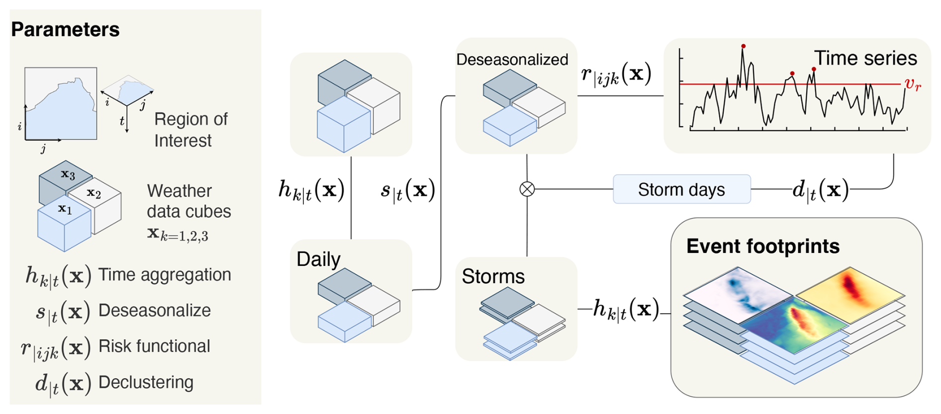
Figure 1 Schematic of the workflow to extract hazard event footprints. Gridded weather data over a region of interest for three variables $\mathbf{x}\in {\mathbb{R}}^{T\times H\times W\times K}$ (indexed k=1, 2, 3) is deseasonalised according to s_|t(x). A risk functional $r_{|ijk}:{\mathbb{R}}^{T\times H\times W\times K}\to {\mathbb{R}}^T$ constructs a time series from the deseasonalised data and a declustering algorithm $d_{|t}\left(r_{|ijk}\right(\mathbf{x}\left)\right)$ identifies storm days. Data cubes are extracted for each storm using the storm days and these are aggregated into storm footprints $\mathbf{x}\in {\mathbb{R}}^{N\times H\times W\times K}$ by applying the temporal aggregation function h_k|t along the time dimension.

2.1.1 Pre-processing the weather data

To handle seasonal effects in weather data, which can bias results and complicate fitting statistical models, deseasonalisation and trend removal is carried out as a pre-processing step. We use the notation $s_{|t}:{\mathbb{R}}^T\to {\mathbb{R}}^T$ to denote a generic deseasonalisation function. Many methods of varying complexity are available, ranging from simple (subtracting climatology or filtering by season) to complex (fitting generalized linear models with seasonal covariates). The choice of method will depend on the data being modelled and the context (see Sect. 3).

2.1.2 Identifying hazard events

The deseasonalised weather data is used to identify hazard events. To do this, we use a severity function $r_{|ijk}:{\mathbb{R}}^{H\times W\times T}\to {\mathbb{R}}^T$ to construct a time series of hazard intensities. The definition of this severity function determines the characteristics of the hazards that will be selected, e.g., calculating the mean or sum of a variable across a region will prioritize widespread events while selecting the maximum over the region will identify events that reach higher peak intensities and may be more spatially localised. More specialised severity functions could also be used, such as for example hazard indices like the storm severity index for windstorms (Dunlop, 2008) or the fire weather index for fire potential (Thompson et al., 2025; van Wagner, 1974).

To identify independent hazard events, a declustering algorithm $d_{|t}:{\mathbb{R}}^T\to {\mathbb{R}}^T$ (Gilleland and Katz, 2016; Coles et al., 2001) is applied to the time series r_|ijk(x). In this framework, hazard days are defined as consecutive days in which r_|ijk(x) exceeds some specified threshold v_r, separated by a specified minimum number of non-exceedences days ℓ_r. The choice of v_r and ℓ_r will depend on the data being modelled and the context. Since we need to fit statistical distributions to the margins, the data should be independent along the sample dimension, which favours using high thresholds v_r and extracting fewer storms. However, small sample sizes in the tails will lead to high variance in the parametric fits, so this trade-off must be handled. The simplest solution is to perform a standard grid search over the space of (v_r,ℓ_r) to select the largest number of events while maintaining independence between the extracted r_|ijk(x) values. Independence can be verified using a standard Ljung–Box test (Ljung and Box, 1978).

Finally, a hazard event set is created by extracting the deseasonalised data corresponding to the declustered hazard days. This creates an event set of smaller spatiotemporal data cubes corresponding to each hazard event and variable. Each data cube will have dimensions $H\times W\times T$, re-purposing the T notation to represent the duration of an arbitrary event. A feature of this approach to event identification is that the extracted variables are sampled conditionally on the occurrence of events, as defined by the severity function. This is intentional: we seek to model the joint behaviour of all variables during hazard events rather than the independent natural extremes of each variable. However, the implications of this for fitting statistical models should be considered and will be discussed later. Broadly, this approach to storm detection bears similarities to the Method of Independent Storms (Cook, 1982) for univariate wind speeds and to the methods of de Fondeville and Davison (2018, 2022) in the spatial setting.

2.1.3 Creating multi-hazard footprints

Each spatiotemporal hazard event can be projected into a 2-D footprint using a temporal aggregation function $h_{k|t}:{\mathbb{R}}^{H\times W\times T}\to {\mathbb{R}}^{H\times W}$. The specific definition of h_k|t will depend on the hazard of interest and how its impact materialises over the event. A measure of cumulative precipitation, for example, may be more relevant for assessing flood risk, while the maximum wind speed may be more relevant for assessing storm damages. Applying a temporal aggregation function to hazard variable creates a set of 2-D event footprints, which can be stacked together to create multi-hazard event footprints with dimensions $H\times W\times K$.

2.2 Transforming the marginal distributions

Figure 2 shows the marginal transformation workflow which takes the set of multi-hazard footprints as input. The marginal distributions of the grid cells are defined along the sample dimension, so there are $H\times W\times K$ marginal distributions. To train a deep learning model we need to standardise these marginals and to properly extrapolate to new extremes, we need to fit an appropriate distribution to their tails.

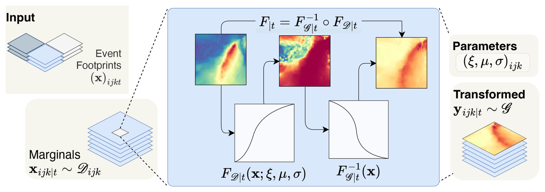
Figure 2 Schematic of the workflow to transform the marginal distributions of the event footprints extracted in Fig. 1 to a standard distribution 𝒢. A suitable parametric distribution is fitted to the extremes of each weather variable along the sample dimension for each variable and location (marginal) ${\mathbf{x}}_{ijk|t}\sim {\mathcal{D}}_{ijk}$. The semiparametric distribution Eq. (1) transforms each marginal to a standard uniform distribution, using the fitted parameters. The quantile function for another distribution 𝒢 then transforms each uniformly distributed marginal such that y∼𝒢.

2.2.1 Marginal extreme value fitting

To generate realistic hazard events, we need to learn the multivariate distribution of the multi-hazard footprints. Critically, we need to learn the marginal and joint distributions of the most extreme values. As Boulaguiem et al. (2022) showed, the ability of a GAN to learn the extremal dependence structure of a dataset can be improved by training it on the empirical distribution functions of its margins. This approach is analogous to classical methods in multivariate extremes, which often disentangle the margins of a multivariate distribution from its dependence structure (Davison et al., 2012). However, Boulaguiem et al. (2022)'s approach relies on fitting generalised extreme value (GEV) distributions to the margins, requiring data in the form of annual block maxima. The use of block maxima creates spatial incoherence, entails significant loss of information, and is unsuitable for modelling the cumulative impact of hazards, such as storms, which materialise over the duration of the event, not just at the peak.

To overcome the limitations of the block maxima approach, we opt for a peaks-over-threshold (POT) approach, allowing us to make more efficient use of data. Heffernan and Tawn (2004, Eq. 1.3) used a semiparametric function, which allowed them to model the entire distribution of the data, using a parametric distribution for the extreme values to guide extrapolation to new extremes, and an empirical distribution for the non-extremes where there is already sufficient data to provide a good approximation. Considering a random variable X and suitably extreme threshold v_X, the semiparametric distribution function can be written in its most general form as:

$$\begin{array}{}\text{(1)}& \stackrel{\mathrm{̃}}{F}\left(x\right)=\left\{\begin{array}{ll}\mathrm{1}-(\mathrm{1}-\widehat{F}(v_X\left)\right)(\mathrm{1}-F_{\mathcal{D}}(x\left)\right)& \text{for }x>v_X\\ \widehat{F}\left(x\right)& \text{for }x\le v_X\end{array}\right.\end{array}$$

where $\widehat{F}$ is the empirical distribution function (ECDF) and 𝒟 is an extreme value distribution used to model the tails. For most applications, 𝒟 will be a generalised Pareto distribution (GPD), as this is the only nondegenerate limiting distribution for exceedances over a high threshold (Coles et al., 2001). In this case, the shape, location, and scale parameters of 𝒟 are denoted by ξ, μ, and σ, respectively. However, we have kept the formulation general to allow for alternative parametric distributions where appropriate (see, for example Harris, 2009). A semiparametric distribution as in Eq. (1) is fitted to all the margins of the multi-hazard event footprints x, transforming them to have standard uniform margins $\mathbf{u}\sim \mathcal{U}(\mathrm{0},\mathrm{1})$.

The event identification approach means that, technically, the distribution of all but one of the margins will be a conditional distribution, conditional on r_|ijk(x) having exceeding the threshold v_r. While in theory conditioning does not violate the assumptions of a GPD fit, the question of whether the conditioned data will be independent and identically distributed is more challenging to address. Although the deseasonalisation and declustering should ensure stationarity and independence of samples, it is still possible that the conditioning will select events arising from different meteorological mechanisms. The POT approach should mitigate this somewhat by isolating the most extreme events, which are more likely to arise from a single dominant mechanism. In Sect. 3 we will use an automated threshold selection method as a further safeguard, which will fail and revert to empirical distributions for any margins where no suitable GPD threshold can be identified. The validity of this approach will depend on the weather variables being modelled and need to be assessed on a case-by-case basis.

2.2.2 Distribution of the training data margins

From a machine learning perspective, transforming the margins to a uniform distribution is a natural standardisation step. However, the uniform probability transform means that the extremes occupy a small region at the edge of the domain. Furthermore, work by Huster et al. (2021) and Wiese et al. (2019) demonstrated that a GAN with a light-tailed latent space struggles to learn the tail behaviour of a heavy-tailed distribution, leading to underestimation of the tails. Huster et al. (2021) developed a GAN with a heavy-tailed latent space to address this issue, but this required replacing the adversarial loss with a custom loss function.

Drawing on these results, we hypothesise that what matters is not the specific tail behaviour of the latent space, but rather that it matches that of the data. A sufficient strategy would therefore be to transform heavy-tailed data to a light-tailed distribution before training, and invert the transformation afterwards. This mirrors common practice in the multivariate extremes literature, where margins are transformed to standard distributions such as the Laplace, Gumbel, Fréchet, or unit Pareto to exploit certain desirable properties (Heffernan and Tawn, 2004; Keef et al., 2009; Quinn et al., 2019). We verify this hypothesis by repeating the experiments of Huster et al. (2021) in the Supplement and find that we can match the results of Huster et al. (2021) using a standard GAN on light tail-transformed data. In Sect. 3, we will explore results of transforming the training data to a standardised distribution 𝒢 and compare the model performance for when 𝒢 is a uniform distribution or another light-tailed distribution.

2.3 Generative model training and sampling

Figure 3 shows the workflow for training the deep generative model and sampling synthetic multi-hazard footprints. The transformed multi-hazard footprints from Fig. 2 are rescaled to take values in the range (0,1) using a custom return period-based scaling function and the three hazard variables, converted to three-channel RGB images in preparation for GAN training. A deep generative network is trained on these images. To create synthetic storm footprints, new samples are generated from the generative model and these are re-scaled using the inverse of the scaling function. The inverse of the transform described in Fig. 2 is used to convert the synthetic footprints back to the scale of the original (deseasonalised) data. The result is a large multi-hazard event set which can be used in risk analysis applications.

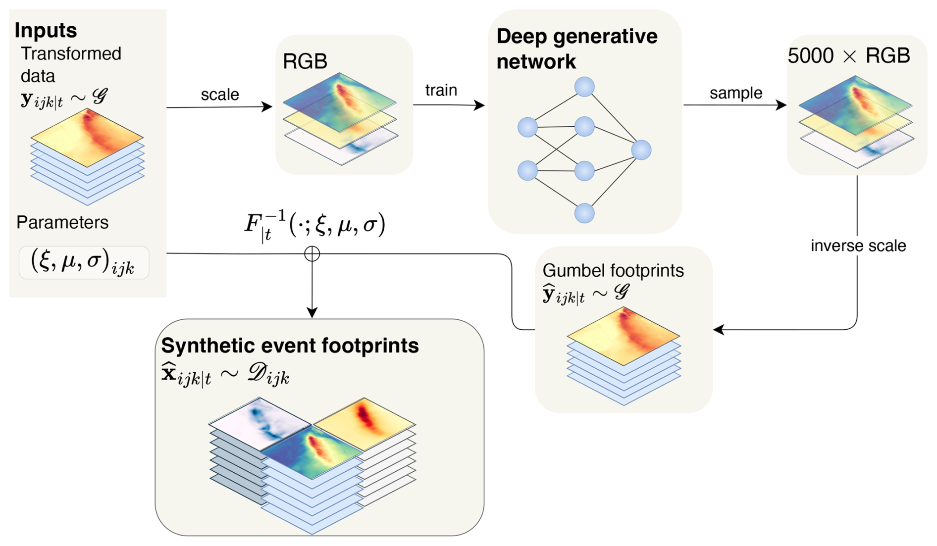
Figure 3 Schematic of the workflow for training the deep generative model. The transformed hazard footprints from Fig. 2 are rescaled to take values in the range (0,1) using a return period-based scaling method (Eq. 2) and converted to three-channel RGB images. A deep generative network is trained on these images. To create synthetic storm footprints, new samples are generated from the generative model and these are re-scaled using the inverse of Eq. (2). The inverse of the probability integral transform (Eq. 1) converts the synthetic footprints back to the scale of the original (deseasonalised) data.

2.3.1 Rescaling footprints be in (0,1)

Depending on the distribution chosen for training 𝒢, the transformed multi-hazard footprints (with marginals y∼𝒢) may require an additional rescaling step to ensure they lie in the range (0,1). A standard rescaling approach is min–max scaling, which maps the largest value of a dataset to 1 and the smallest value to 0. But this would prevent the GAN from generating values outside the range of the training data, which is our goal.

An alternative approach that allows us to specify a sensible maximum range for the generated data, using only the training data, is to set the maximum range using quantiles of the training distribution 𝒢, which we can specify to correspond specific return periods. For example, we can set it so that the maximum possible value our method can produce, at any point on the domain, corresponds to an intensity that is on average exceeded once every R events at that point (or similarly, once every $R^{\prime }=\mathit{\lambda }R$ years, with λ the number of events per year). For the distribution 𝒢, the minimum and maximum values associated with R are $F_{\mathcal{G}}^{-\mathrm{1}}(\mathrm{1}/R)$ and $F_{\mathcal{G}}^{-\mathrm{1}}(\mathrm{1}-\mathrm{1}/R)$, respectively. Following this approach, the data can be rescaled according to

$$\begin{array}{}\text{(2)}& y^{\prime }={\displaystyle \frac{y-F_{\mathcal{G}}^{-\mathrm{1}}(\mathrm{1}/R)}{F_{\mathcal{G}}^{-\mathrm{1}}(\mathrm{1}-\mathrm{1}/R)-F_{\mathcal{G}}^{-\mathrm{1}}(\mathrm{1}/R)}},\end{array}$$

assuming that R is sufficiently large that $F_{\mathcal{G}}^{-\mathrm{1}}(\mathrm{1}/R)$ is smaller than the smallest value in the training data and $F_{\mathcal{G}}^{-\mathrm{1}}(\mathrm{1}-\mathrm{1}/R)$ is larger than the largest value in the training data. While this will result in the same maximum and minimum values across the 𝒢-distributed training data, it will map back to different values in physical space.

After rescaling, the weather fields are stacked such that each multivariate footprint is now a three-channel tensor. Finally, it is converted to an RGB image, ready to feed into a generative model.

2.3.2 Generative adversarial network

In theory, this framework is agnostic to the choice of deep generative model, meaning common models like variational auto-encoders (Kingma and Welling, 2013), diffusion models (Ho et al., 2020), or flow-based models (Kobyzev et al., 2021) could be used instead of GANs. In practice, however, historical weather datasets such as ERA5 generally contain fewer than 100 years of data, and for rare events, this does not provide enough extreme events to train standard deep generative models.

Some GANs have been developed to work well with small datasets, such as FastGAN (Liu et al., 2021) and StyleGAN2-ADA (Karras et al., 2020), which use a self-supervised discriminator and adaptive discriminator augmentation (ADA), respectively, to prevent overfitting. Augmentation regularises the discriminator by adding semantics-preserving augmentations (e.g. additive noise, rotations, isometric scaling, saturation changes) to all samples. When combined with additional differentiable augmentation (DA), StyleGAN2-ADA successfully learned the distribution of a dataset of only 100 images from scratch (Karras et al., 2020; Zhao et al., 2020). In Sect. 3, we will use StyleGAN2-ADA with differentiable augmentations (StyleGAN2-ADA+DA) to train a generative model on a set of multi-hazard footprints.

2.4 Evaluation and benchmarking

The quality of generated event footprints will be evaluated against the training data according to several criteria, which can be broadly categorized into three groups: (i) the distribution of event severity; (ii) marginal distributions; and (iii) multivariate dependence structures.

2.4.1 Evaluation metrics

To measure the similarity between any two distributions, we will use the Wasserstein distance. The Wasserstein distance, also known as the Earth Mover's Distance, measures the minimum cost of transporting mass to transform one distribution into another. For one-dimensional distributions, the Wasserstein distance can be computed from distribution P to distribution Q as

$$\begin{array}{}\text{(3)}& W(P,Q)=\underset{\mathbb{R}}{\int }\left|P\right(x)-Q(x\left)\right|\mathrm{d}x.\end{array}$$

The Wasserstein distance is non-negative and takes a value of zero if and only if P and Q are the same distribution.

To assess whether the dependence structures are being learned correctly, we will first calculate dependence metrics between pairs of marginal distributions for each dataset. We will then compare the distributions of the generated dependence metrics to those of the training data. We will use Pearson correlation and mean-squared-error to assess the similarity between the calculated dependence metrics.

To measure the dependence between non-extreme values, we will use the Pearson correlation coefficient to measure linear agreement between the variables. To measure the level of extremal dependence between two variables X₁∼F₁ and X₂∼F₂, the extremal correlation between them, χ, above a fixed high threshold u can be written as Coles et al. (1999, p. 346),

$$\begin{array}{}\text{(4)}& \begin{array}{rl}\mathit{\chi }\left(u\right)& ={\displaystyle \frac{\mathrm{Pr}\left(F_{\mathrm{1}}\right(X_{\mathrm{1}})>u,F_{\mathrm{2}}(X_{\mathrm{2}})>u)}{\mathrm{Pr}\left(F_{\mathrm{1}}\right(X_{\mathrm{1}})>u)}}\\ & ={\displaystyle \frac{\mathrm{Pr}\left(F_{\mathrm{1}}\right(X_{\mathrm{1}})>u,F_{\mathrm{2}}(X_{\mathrm{2}})>u)}{\mathrm{1}-u}}.\end{array}\end{array}$$

We will use the simple empirical estimator for χ(u), which can be calculated from a sample of size n as

$$\begin{array}{}\text{(5)}& \widehat{\mathit{\chi }}\left(u\right)={\displaystyle \frac{{\sum }_{i=\mathrm{1}}^n\mathbb{1}\mathit{\left\{}{\widehat{F}}_{\mathrm{1}}\right(X_{\mathrm{1}i})>u,{\widehat{F}}_{\mathrm{2}}(X_{\mathrm{2}i})>u\mathit{\}}}{{\sum }_{i=\mathrm{1}}^n\mathbb{1}\mathit{\left\{}{\widehat{F}}_{\mathrm{1}}\right(X_{\mathrm{1}i})>u\mathit{\}}}},\end{array}$$

where ${\widehat{F}}_i$ indicates the empirical distribution function of variable X. The true extremal correlation χ is defined as the asymptotic limit of χ(u) as u→1. The extremal correlation takes values in [0,1], where χ=0 indicates asymptotic independence and χ>0 indicates asymptotic dependence. The higher the value of χ, the stronger the extremal dependence between the two variables. In practice, however, a finite, high threshold u can be used to approximate χ.

The χ metric tells us the strength of extremal dependence, and it is often supplemented by the $\stackrel{\mathrm{‾}}{\mathit{\chi }}$ metric, which measures the strength of asymptotic independence – where the variables maintain some dependence at finite, high levels but are ultimately independent. To assess the strength of asymptotic independence, we can use the $\stackrel{\mathrm{‾}}{\mathit{\chi }}$ metric, which is defined as Coles et al. (1999, p. 348),

$$\begin{array}{}\text{(6)}& \stackrel{\mathrm{‾}}{\mathit{\chi }}\left(u\right)={\displaystyle \frac{\mathrm{2}\log (\mathrm{1}-u)}{\log \mathrm{Pr}\left(F_{\mathrm{1}}\right(X_{\mathrm{1}})>u,F_{\mathrm{2}}(X_{\mathrm{2}})>u)}}-\mathrm{1}.\end{array}$$

2.4.2 Benchmarking

To benchmark the performance of the method, we compare it to a widely used model for multivariate extremes: the Heffernan and Tawn (2004) model. The model learns the conditional distribution of a set of variables, given that one of them exceeds a high threshold. For two variables standardised to Gumbel-distributions Y_i and Y_j, the probability that Y_j exceeds a high threshold u given that Y_i exceeds u is given by Heffernan and Tawn (2004, Eq. 4.1):

$$\begin{array}{}\text{(7)}& Y_j=a\left(Y_i\right)+b\left(Y_i\right)Z,Z\sim G_{|i}\end{array}$$

where G_|i is the residual distribution after normalising Y_j with the scalars a(Y_i) and b(Y_i). The form of G_|i may vary, and depends on whether the margins of the residual distribution are asymptotically dependent. This naturally scales up to the multivariate case, where we can model the distribution of n other variables $\mathbf{j}=\mathrm{1},\mathrm{\dots },n$, modelling Y_j conditional on Y_i exceeding u.

3 Application: Bay of Bengal storms

We apply the method to a case study of storms in the Bay of Bengal, a region highly exposed to tropical cyclones, which are not well characterised by existing event sets (Meiler et al., 2022). We model three variables that determine the impact of tropical cyclones: wind speed, precipitation, and atmospheric pressure at sea-level, which affects the elevation of storm surges.

3.1 Data

Our dataset consists of hourly gridded weather data from the ERA5 reanalysis product from 1940 to 2022 (Hersbach et al., 2023a). We extract the northerly and easterly components of 10 m wind speeds (m s⁻¹), total precipitation (m), and atmospheric pressure at sea level (Pa) over the region and calculate wind speed as the ℓ₂-norm of the northerly and easterly components of the 10 m wind speeds.

3.2 Event identification and footprint creation

Since deseasonalisation and risk estimation are not the central contributions of this work, we opt for simple methods to avoid unnecessary complexity. Seasonal effects are removed from the weather data using the deseasonalisation function s_|t(x), which computes monthly medians for each margin and subtracts them, yielding a time series of climatological anomalies. Storm events are identified using the daily maximum 10 m wind speeds over the domain $r_{|ijk}\left(\mathbf{x}\right)={max}_{k=\mathrm{0}|ij}\left(\mathbf{x}\right)$ (where k=0 indicates the wind speed variable). Taking the domain maximum prioritises strong, localised wind storms (including tropical cyclones) over more widespread, low-intensity events.

Figure 4 maps the mean and standard deviation of wind speeds alongside the frequency with which each grid cell contributed the domain maximum on a storm day. While mean winds and wind variance exhibit strong spatial patterns, storm-triggering pixels are distributed relatively uniformly across the domain, predominantly offshore. Over the 1941–2022 period, no single pixel triggered more than 16 separate events (1.2 % of events). While the distribution of storm-triggering pixels is relatively even, some spatial variation in sampling frequency is also expected and acceptable: locations regularly exposed to strong winds should trigger storms more frequently, correctly reflecting the spatial distribution of wind hazard.

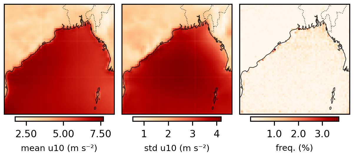
Figure 4 Map of grid cells that triggered storm events, based on being the site of the maximum wind speed over the domain on a given day.

To create 2-D multi-hazard footprints, we define a function h_k|t(x) for each weather variable k=1, 2, 3. For wind speeds, $h_{\mathrm{1}|t}\left(\mathbf{x}\right)={max}_{|t}\left({\mathbf{x}}_{\mathrm{1}}\right)$, extracting the peak wind speed per pixel over the duration of each event; for precipitation $h_{\mathrm{2}|t}\left(\mathbf{x}\right)={\sum }_{|t}\left({\mathbf{x}}_{\mathrm{2}}\right)$, extracting the cumulative precipitation over the events duration; and for sea level pressure $h_{\mathrm{3}|t}\left(\mathbf{x}\right)={min}_{|t}\left({\mathbf{x}}_{\mathrm{3}}\right)$, extracting the lowest sea-level pressure over the event's duration.

3.3 Marginal transformations

We fit the semiparametric distribution Eq. (1) to the margins of the wind speed, precipitation, and (negated) sea-level pressure footprints and in line with Heffernan and Tawn (2004), we use a generalised Pareto distribution (GPD) as the parametric tail model. Threshold selection for the GPD for each of the 12 000 margins is done using the ForwardStop method of Bader et al. (2018). The method uses the Anderson–Darling goodness-of-fit test to sequentially test the hypothesis of a GPD fit for a range of candidate thresholds, using a rejection rule that smoothes the p-values of the independent tests, controlling the likelihood of false discoveries.

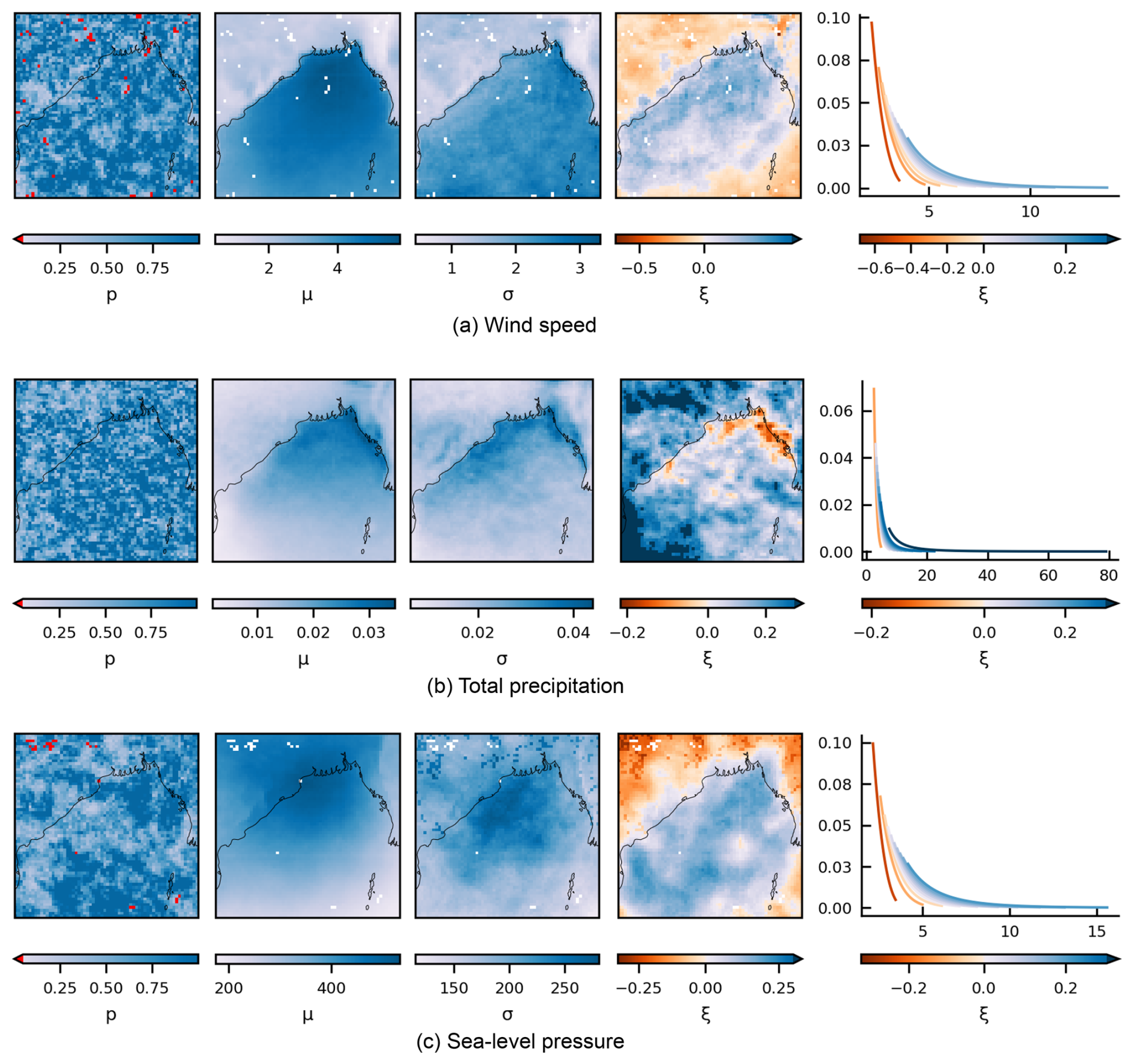
Figure 5 Left panels: fitted parameters for the marginal distributions of weather variables over the Bay of Bengal during storms, showing adjusted p-values for Anderson–Darling (AD) goodness-of-fit tests (left column), thresholds μ, scale parameters σ, shape parameters ξ. White pixels indicate locations where the AD test failed and empirical distributions were used instead. Right column: density plots of each distribution for a range of tail shapes – with (μ,σ) fixed at (0,1). Shown are: generalised Pareto parameters for (a) peak wind speeds, (b) total precipitation, and (c) low pressure.

Figure 5a–c shows the fitted parameters for each of the wind, precipitation, and sea-level pressure event sets. For precipitation, the Bader et al. (2018) method successfully selected a threshold for all margins, while for wind speed and sea level pressure, it failed to select thresholds for 54 and 35 margins, respectively. The rejected margins were fitted using entirely empirical distributions. These pixels are shown as red/white pixels in the fitted parameter plots.

Figure 5 shows that the GPD parameters vary relatively smoothly across the domain for all three variables, with a marked difference between onshore and offshore regions. The shape parameter estimates show the highest variation, with wind and sea-level pressure assigned predominantly negative shape parameters over land, suggesting the existence of an upper bound for wind speeds and a lower bound for sea-level pressure in these regions. Similarly, precipitation is assigned some negative shape parameters along the northern coastline. The existence of upper bounds for wind and rainfall have been much-contested in the literature (Harris, 2005; Serinaldi and Kilsby, 2014); however, and such conclusions should be treated with caution. Additionally, a large patch of very heavy-tailed precipitation is visible in the southwestern corner of the domain. While beyond the scope of this study, it is possible that the fits could be made more robust by fitting a nonstationary model over the domain, allowing us to effectively “borrow strength” between pixels (Davison et al., 2012; Huser and Wadsworth, 2022, pp. 167, pp. 2).

Applying the semiparametric distribution functions Eq. (1) with the parameters shown in Fig. 5, the transformed variables $\mathbf{u}=\stackrel{\mathrm{̃}}{F}\left(\mathbf{x}\right)$ have a standard uniform distribution. But as discussed in Sect. 2, training a GAN on data with uniform margins can lead to poor representation of tail behaviour. We apply an additional transformation to the data to transform it to a standard light-tailed distribution, using the quantile function of the target distribution. To investigate the effects of this transformation compared to the standard approach of training a GAN on rescaled data or Boulaguiem et al. (2022)'s approach using uniform margins, we train separate GANs on data using (i) the original data, rescaled to (0,1); (ii) uniform margins; (iii) Gaussian margins; and (iv) Gumbel margins. While the Gaussian and Gumbel distributions are both light-tailed distributions that belong to the same (Type I) domain of attraction, their subasymptotic behaviour is different, which we hypothesise may lead to different performance.

To rescale the training data to the interval (0,1) for training a deep learning model, we use the return period-based rescaling method described in Sect. 2. We use a 1-in-R = 10 000 event return level to specify the maximum value any generated marginal can reach (choosing event-based rather than year-based scaling for simplicity). This is converted into a maximum value of $\mathrm{1}-\mathrm{1}/R$ for the uniform distribution and $F_{\mathcal{G}}^{-\mathrm{1}}(\mathrm{1}-\mathrm{1}/R)$ for the Gaussian and Gumbel distributions. The lower bounds are calculated analogously, i.e., using a minimum value of $\mathrm{1}/R$ for the uniform distribution and $F_{\mathcal{G}}^{-\mathrm{1}}(\mathrm{1}/R)$ for the Gaussian and Gumbel distributions. As a heuristic, the no-transform data is rescaled to (0,1) by setting 1 to correspond to the maximum value multiplied by $\log \left(R\right)/\log \left(N\right)$, where N is the number of independent hazard events – approximating the ratio of the R-event to N-event maximum under Gumbel tails. While we note this is inexact, it is sufficient for our comparative purposes.

3.4 Generative modelling

The final training datasets consisted of 1249 multi-hazard storm footprints. Although we initially attempted to train a Wasserstein GAN with gradient penalty (Arjovsky et al., 2017; Gulrajani et al., 2017) on the 1249-event dataset, we found that the GAN became biased towards the more common, less spatially coherent storms. To address this, we used the GAN that has been specifically developed for small datasets, the StyleGAN2-ADA model, with additional differentiable augmentation (Karras et al., 2020; Zhao et al., 2020), which can produce good results on as few as 100 training samples.

We filtered the data to only include storms with a maximum wind speed anomaly r_|ijk(x) exceeding 15 m s⁻¹, resulting in a dataset of 150 storms. We trained the StyleGAN2-DA on the 150 most extreme storms for 2013 epochs (i.e., so that it had sampled images 300 000 times). This took approximately four hours on an NVIDIA GeForce GTX 1080 Ti GPU. The GAN was then used to generate 500 years of synthetic hazard events, which for storms with a yearly rate of λ=1.82, corresponds to 914 multi-hazard footprints.

3.5 Results

3.5.1 Visual appearance

Ranking scores according to the severity function, as defined by the domain-maximum wind speed $r_{|ijk}\left(\mathbf{x}\right)={max}_{k=\mathrm{0}|i,j}\left(\mathbf{x}\right)$, Fig. 6 compares the 16 most severe storm footprints derived from the ERA5 dataset (top rows) with the most extreme footprints generated using the GAN (bottom rows) for each of the four training configurations: rescaling-only, uniform margins, Gaussian margins, and Gumbel margins. Corresponding figures for sea-level pressure and precipitation fields are also provided in the Supplement.

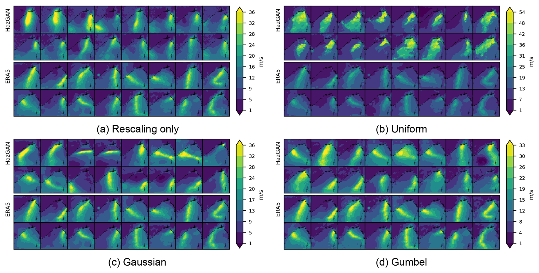
Figure 6 Comparison of wind speed footprints during storms in the Bay of Bengal for ERA5 training data vs. GAN-generated samples. Shown for a GAN trained on (a) margins rescaled to [0,1] in the usual way, (b) margins transformed to uniform, (c) margins transformed to Gaussian, and (d) margins transformed to Gumbel.

Qualitatively, the rescaled and Gumbel footprints look most similar to the ERA5 training data. Uniform-trained events are more extreme, overly-widespread, and do not exhibit the gradual decay in intensity with distance from the storm centre that would normally be expected. The footprints generated by standard rescaling also look reasonable, although the track shapes appear more simple and ellipsoidal than those produced by the Gumbel or Gaussian-trained models. The latter exhibit longer tracks and more pronounced changes of direction, better capturing the curved trajectories seen in the ERA5 reference footprints.

3.5.2 Marginal distribution fits

To assess the GAN's ability to capture marginal distributions, we calculate the Wasserstein distance between the generated and training data for each margin using Eq. (3), scaling by the standard deviation of the training data distribution. The average rescaled Wasserstein distance across all margins is 0.57 for the rescaled model, 0.21 for the uniform model, 0.13 for the Gaussian model, and 0.14 for the Gumbel model, indicating that the Gaussian and Gumbel models are overall better capturing the marginal distributions of the training data.

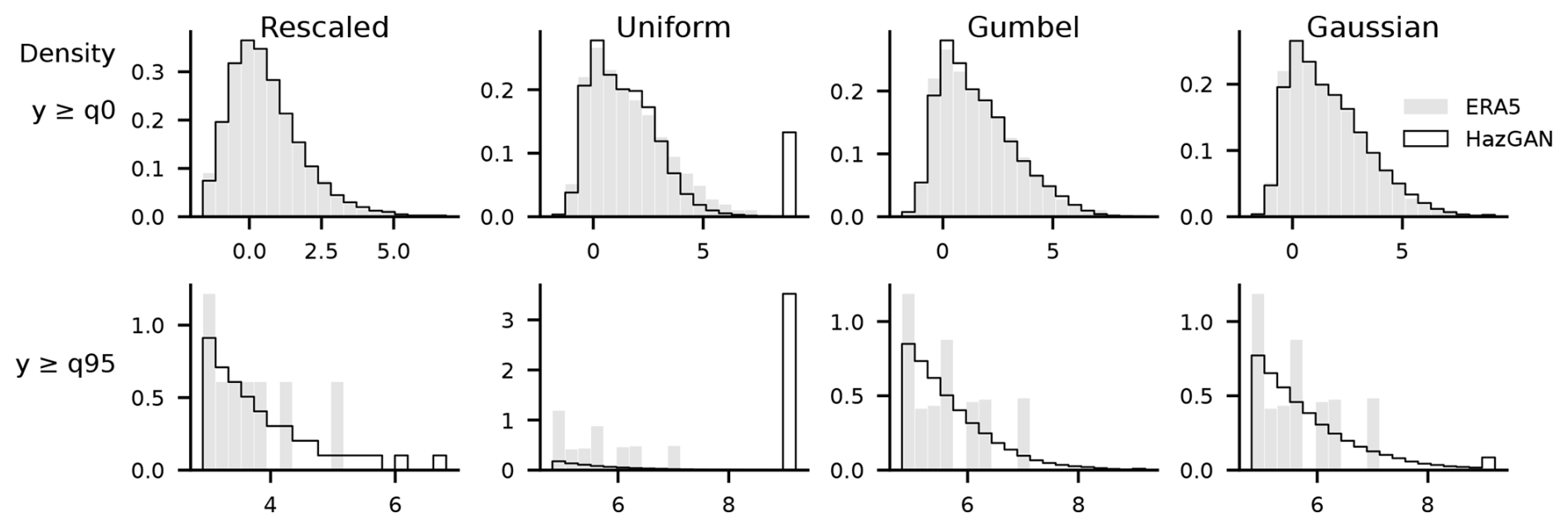
Figure 7 Flattened distribution of wind speed pixels for the data generated using each model. All variables transformed to Gumbel to enable cross-comparison.

To assess how well each model captures the overall distribution of pixel values, Fig. 7 shows the flattened distributions of all pixels, transformed to Gumbel scale to enable cross-comparison. The uniform-trained model shows a pronounced spike at the maximum value, suggesting the GAN attempted to extrapolate beyond its allowed range, saturating at the 10 000-year return period. The Gaussian-trained model exhibits the same behaviour, though far less severely. The Gumbel and rescaled models avoid this saturation: the Gumbel model produces the smoothest tail decay, while the rescaled model shows a more stepped distribution.

3.5.3 Storm event distribution fits

To assess how well the GAN captures the storm severity distribution, we again calculate the severity r_|ijk(x) for each storm in the training and generated data and compare their distributions in Fig. 8. The rescaled and uniform-trained models perform poorly here with high Wasserstein distances (3.7 and 16.8, respectively) compared to the Gaussian and Gumbel models (0.71 and 1.0, respectively).

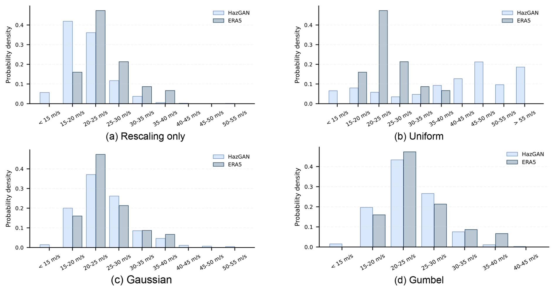
Figure 8 Comparison of the distribution of storm intensities in the Bay of Bengal between 500 years of GAN-generated and 81 years of ERA5 event footprints. Storm intensities are assigned according to the domain-wide maximum wind speed during each storm. Shown for GANs trained on (a) data rescaled in the usual way for deep learning; (b) data transformed to a uniform distribution via a probability transform; (c) data transformed to a Gaussian distribution; and (d) data transformed to a Gumbel distribution.

3.5.4 Spatial dependence structures

To assess how the model is learning the spatial dependence structures, we estimate the tail dependence coefficients $\widehat{\mathit{\chi }}\left(u\right)$ (choosing u=0.8 based on initial data exploration) between all pairs of pixels across the domain, generating for each variable a 4096×4096 matrix for each of the four generated datasets (Fig. 9). We quantify the level of agreement between the ERA5 and GAN-generated correlation structures by calculating the Pearson correlation and mean absolute error (MAE) between the two extremal correlation matrices. The rescaled model performs worst, with a correlation of 0.380 (MAE = 0.309) between the ERA5 and GAN-generated correlation fields for wind speed, while the uniform, Gaussian, and Gumbel models perform much better, with correlations of 0.839 (MAE = 0.088), 0.837 (MAE = 0.089), and 0.857 (MAE = 0.083), respectively.

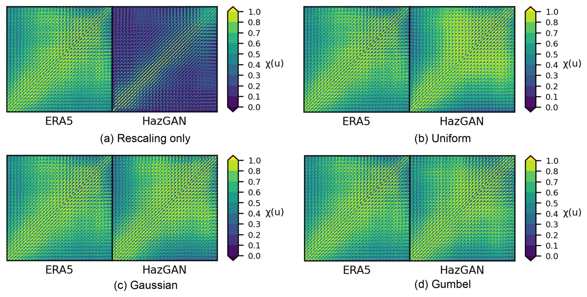
Figure 9 Pairwise spatial extremal correlation estimates at $\widehat{\mathit{\chi }}\left(\mathrm{0.8}\right)$ for 10 m wind speed anomalies during storms across the Bay of Bengal.

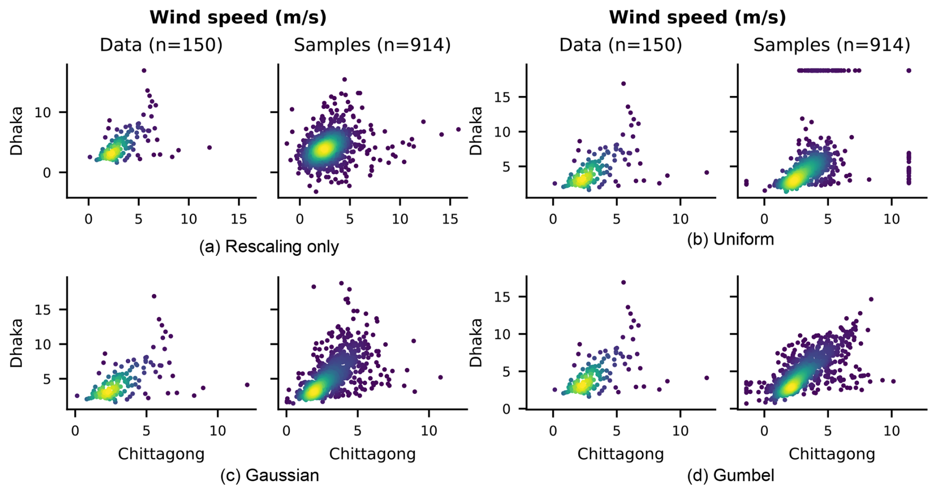
Figure 10 Scatter plots comparing the bivariate distribution of 10 m wind speed anomalies between the cities of Dhaka and Chittagong in Bangladesh.

For a more detailed view of bivariate spatial relationships, Fig. 10 shows scatter plots of 10 m wind speed anomalies between Chittagong and Dhaka, two cities in Bangladesh. The rescaling-only model produces a noticeably simpler, more ellipsoidal dependence structure than is seen in the ERA5 data, while the uniform-trained model struggles to resolve marginal extremes, producing clustering visible at the boundaries. Both the Gaussian and Gumbel-based models show considerably better agreement with the observed dependence structure, with the Gaussian model appearing to provide the closest match. Similar results were observed for all other variables and pairs of locations tested.

3.5.5 Multivariate dependence structures

Figure 11 maps the extremal correlation estimates $\widehat{\mathit{\chi }}\left(\mathrm{0.8}\right)$ between 10 m wind speed and total precipitation across the Bay of Bengal for training data and the four GAN-generated datasets. The GANs trained on uniform, Gaussian and Gumbel margins show the best agreement with the ERA5 data, with Pearson correlations of 0.664 (MAE = 0.104), 0.666 (MAE = 0.089) and 0.705 (MAE = 0.08), respectively. The rescaling-only and uniform-trained model performs much worse, with correlation of 0.193 (MAE = 0.117). In all cases, the generated data had a tendency to overestimate the strength of the inter-variable dependence, with the mean overestimation (across all pairs of variables and locations) of 0.292 (uniform), 0.256 (Gaussian), 0.205 (Gumbel), and 0.241 (rescaling-only). The Gumbel-trained model performs best here, with the lowest mean error and highest correlation with the training data, while the uniform-trained model performs worst. We observe that these scores are slightly lower than the spatial dependence scores, which may be due to the architecture of StyleGAN prioritising spatial relationships or because the inter-variable dependence structure is more complex and harder to learn than the spatial dependence structure.

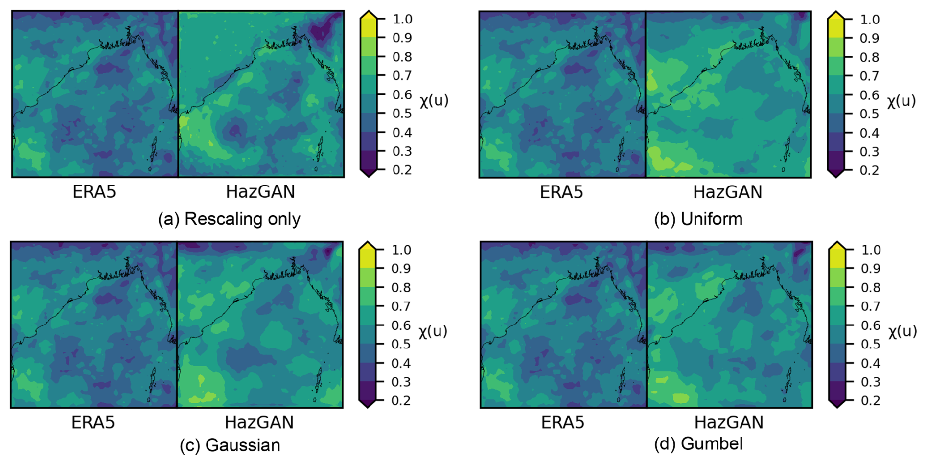
Figure 11 Inter-variable extremal correlation estimates $\widehat{\mathit{\chi }}\left(\mathrm{0.8}\right)$ for 10 m wind speed and total precipitation over the Bay of Bengal.

3.5.6 Benchmarking against the Heffernan and Tawn (2004) model

We choose the Gaussian model as the best-performing model and compare its performance to the Heffernan and Tawn (2004) conditional exceedance model, which is provided in R's texmex package (Southworth et al., 2024). In this package, the mexDependence function integrates the GPD fitting of Eq. (3.2) and the fitting of the dependence model Heffernan and Tawn (2004, Eq. 4.1) into a single function, but our data has already been transformed to a uniform scale using Eq. (1), so we customise the mexDependence function to skip the GPD-fitting step and directly accept data on the uniform scale.

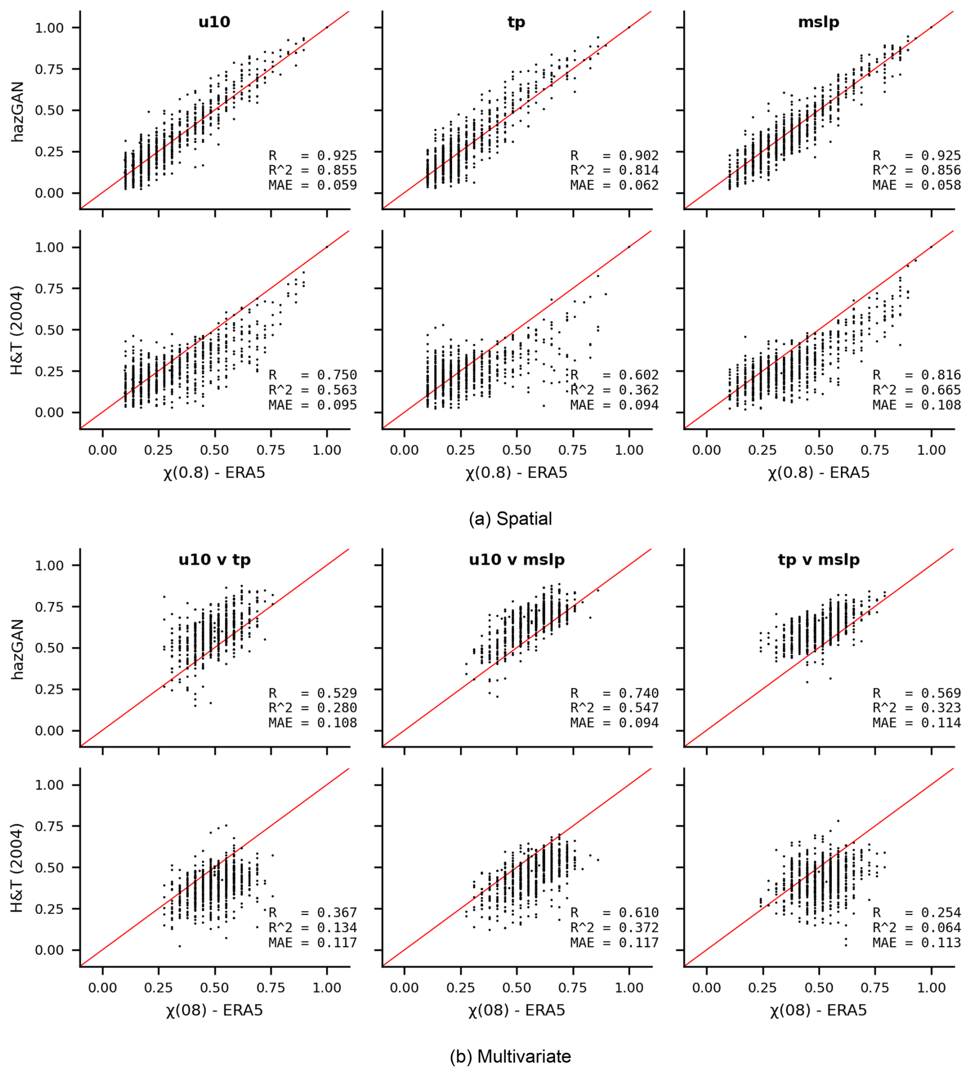
Figure 12 Comparison of how hazGAN and the Heffernan and Tawn (2004) model capture the (a) spatial dependence and (b) multivariate dependencestructures of the ERA5 training data. The x-axes show $\widehat{\mathit{\chi }}\left(\mathrm{0.8}\right)$ estimates for 1000 randomly sampled pairs of variables in the training data and the y-axes show the $\widehat{\mathit{\chi }}\left(\mathrm{0.8}\right)$ estimates from the same variables in the synthetic data.

Using the dataset of the top-150 storms, we randomly sample 1000 points across the domain and fit a conditional exceedance model between (i) different weather variables at that point, and (ii) for the same weather variable between that location and a second, randomly sampled, location. We then use the fitted model to generate 500 years of synthetic data, and calculate $\widehat{\mathit{\chi }}\left(\mathrm{0.8}\right)$ between the generated and training data. Figure 12a plots the distribution of spatial extremal correlations for each weather variable and Fig. 12b plots the inter-variable extremal correlations for all combinations of wind speed, precipitation, and sea-level pressure.

Both models struggle more to model the inter-variable dependence structure than the spatial structure, suggesting that the inter-variable dependence structure is indeed more challenging to learn. Nonetheless, the GAN achieved higher correlations and lower MAE compared to the training data than the Heffernan and Tawn (2004) model for both spatial and inter-variable dependence. Overall, this result is encouraging, particularly because the hazGAN model learns the full joint distribution of all variables and locations simultaneously, whereas the Heffernan and Tawn (2004) model is learning pairwise relationships separately so does not capture higher-order dependencies. As a result, the GAN may be able to borrow strength across the full dataset, enabling it to learn a more accurate dependence structure, while the Heffernan and Tawn (2004) model fits many separate models, each with less data. In the future, it would be interesting to compare the GAN to spatial models for extremes, such as r-Pareto processes (de Fondeville and Davison, 2018), which are designed to model extremal spatial fields. However, we consider this beyond the scope of the current work, which aims only to demonstrate the effectiveness of the hazGAN approach.

4 Use case: Spatial risk assessment for mangrove forests in the Bay of Bengal

To illustrate an application in risk analysis, we use the event set generated by the Gaussian-based model to estimate risk to mangrove forests from storms impacting the Bay of Bengal. To model storm risk to mangrove forests, we need to model the joint distribution of both wind and precipitation and to estimate aggregate impacts over a domain as large as the Bay of Bengal, we need a model that generates spatial events with the right dependence structure. Thus, this problem necessitates a new approach to event set generation that can account for spatial and multivariate dependencies, making it a suitable test case for our model.

4.1 Implementation details

To estimate damages to the mangroves from the multivariate storm footprints we use a bivariate logistic regression model trained on global historical mangrove damages and tropical cyclone characteristics (Mo et al., 2023; Bunting et al., 2022). The model predicts the probability that a mangrove patch is damaged, conditional on local winds and precipitation. A patch is defined as “damaged” if it experiences a drop in enhanced vegetation index (EVI) exceeding 20 % in the aftermath of a storm. Further details of the mangrove fragility function and relevant calculations are provided in the Supplement. We use the 500 years of wind and precipitation footprints generated in Sect. 3 as input to the mangrove fragility model.

To illustrate the implications of ignoring the spatial dependence structure of climate hazards, two more synthetic datasets are constructed: a dataset that ignores all dependence across the region (independence assumption), and a dataset that assumes total dependence across the region (total dependence assumption). The total dependence assumption is the assumption implicit when return period hazard maps are treated like true events, while the independence assumption is implicit when regional risks are modelled separately and the results aggregated (Metin et al., 2020). These assumptions will lead to somewhat exaggerated results: modelling the dependence structure of hazards across space completely independently or dependently is an extreme assumption; however, they illustrate the critical importance of modelling the dependence structure of hazards when estimating risk, and the significant potential for bias when this is neglected.

4.2 Results

Figure 13 shows the risk profile for widespread mangrove damages over the Bay of Bengal, plotting the expected area of mangrove forest damaged against event return period. The return period is calculated as a function of the total mangrove damage area (see the Supplement for calculation details). The figure also displays risk profiles for hazard events generated under independence and total dependence assumptions, which clearly introduce significant bias even at small return periods.

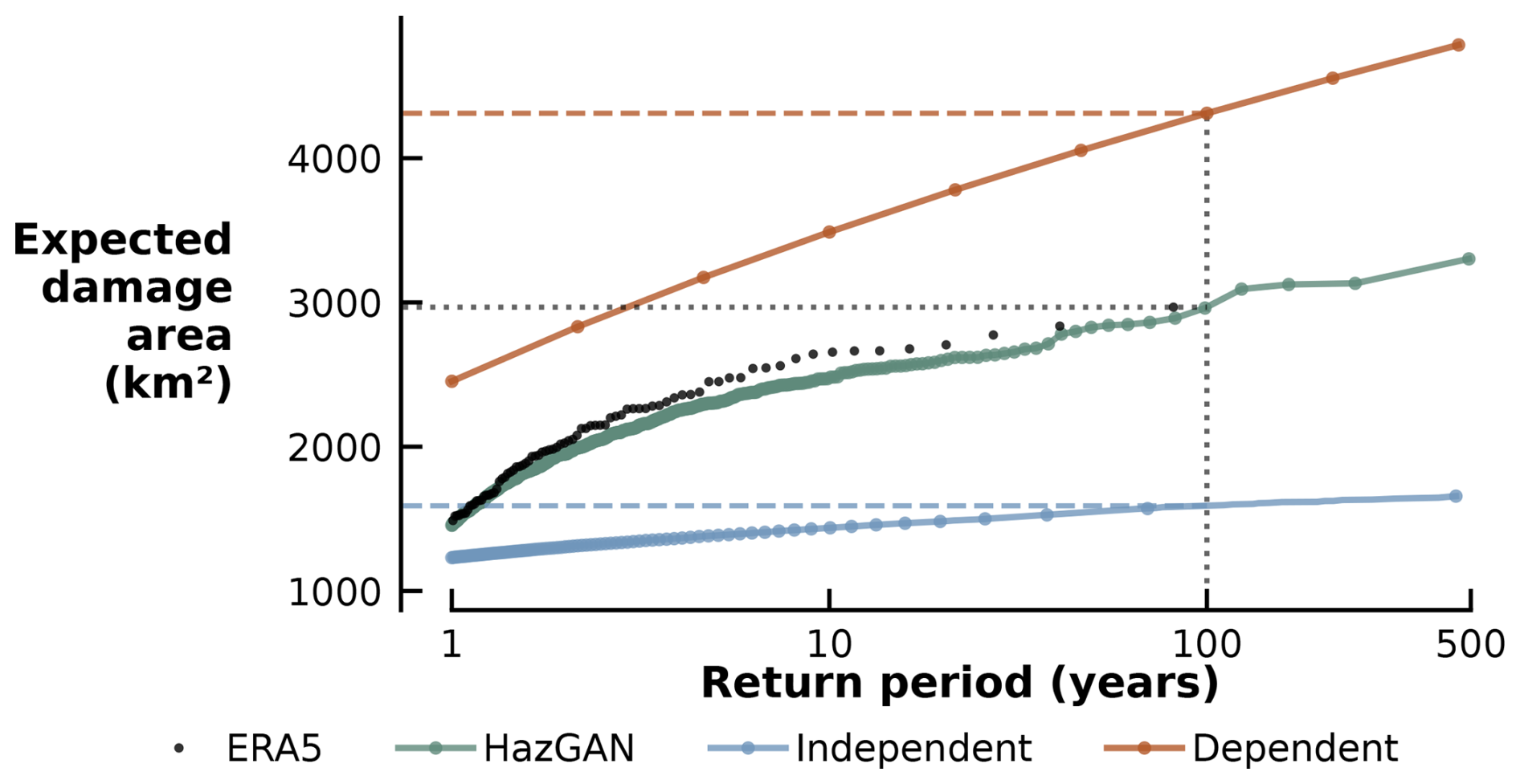
Figure 13 Risk profiles showing the expected total area of mangrove forest damaged by storms of different return periods for ERA5 and GAN-generated storm footprints. Also shown are risk profiles for the two simplifying assumptions of total dependence or independence across the domain, where a total dependence assumption is analogous to using return period maps to calculate risk profiles. With a total area of mangrove forest across the bay of 9917 km² in 2020 (Bunting et al., 2022), 2000 km² corresponds to approximately 20 % and 4000 km² corresponds to approximately 40 % of the total area of mangrove forest present.

Applied to the ERA5 data, the logistic model predicts 2451.21 km² (25 %) of the 9917 km² mangrove forest in the region to be damaged by a five-year storm event and 2967.11 km² (30 %) to be damaged by a 100-year storm event. A five-year storm generated by the GAN produces damages of 2309.12 km² (23 %) and a 100-year storm damages 2891.09 km² (29 %). A 100-year storm under the total dependence assumption predicts damage to 43 % of the mangrove forest in the Bay of Bengal, significantly overestimating the risk. For a 500-year event, the GAN-generated data predicts damage to 33 % of mangrove forest in the region (3301.93 km²); the dependence assumption-generated data predicts damage to 48 % of mangrove forests (4785.14 km²); and the independence assumption-generated data predicts damage to only 16 % of the mangrove forests (1660.71 km²).

Table 1 Expected damage area and return period deviations for GAN, independent, and dependent generated samples.

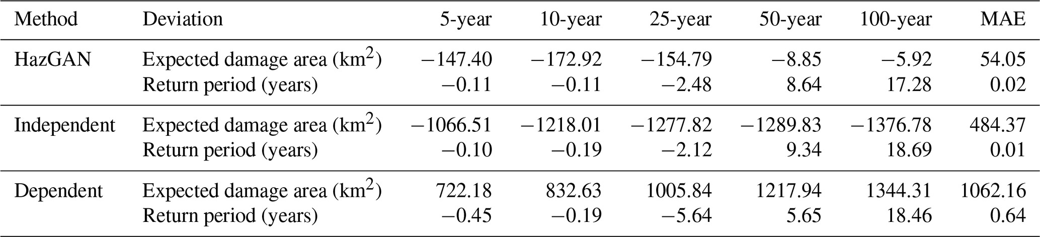
Table 1 reveals that while the GAN-generated dataset appears to underestimate total expected damages with a mean absolute error of 54 km² across all return periods (reaching up to 173 km² for 10-year events), this bias remains an order of magnitude smaller than the independent dataset's systematic underestimation (mean absolute error of 484 km²) and the dependent assumption dataset's systematic overestimation (mean absolute error of 1062 km²).

To visualise the qualitative difference between modelling the dependence structure and assuming total or no dependence, Fig. 14 shows, for the ERA5 and synthetic datasets, a sample corresponding to a 1-in-75 year return period. The extreme winds under realistic events are spatially clustered, while the dependent assumption distributed extreme winds evenly across the entire region, resulting in far more widespread and unrealistic disruption estimates. The independence assumption shows no spatial coherence and so underestimates the impacts of spatially coherent events. By construction, the independence assumption exhibits no spatial coherence, hence underestimating the impact of spatially coherent events.

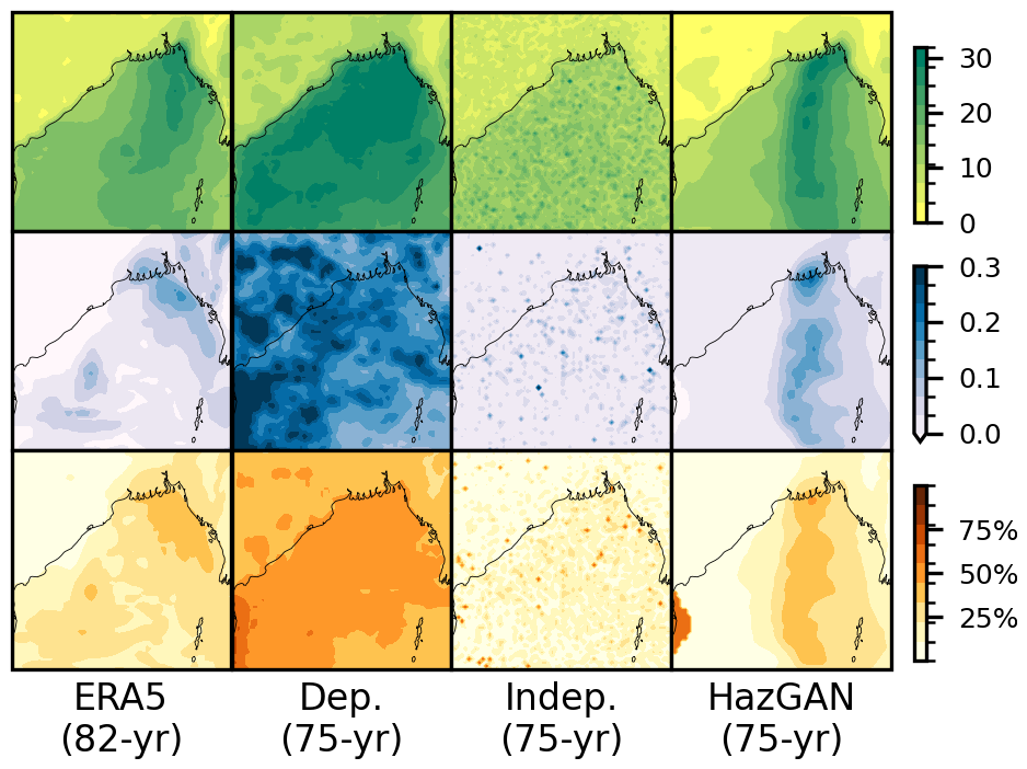
Figure 14 Footprints for events with approximately 1-in-75 year return period mangrove damages for the ERA5 and hazGAN-generated datasets, as well as samples from the two simplifying assumptions of total dependence or independence between all variables.

5 Discussion

5.1 Main findings

A key result of this work was the insight that training a GAN (with Gaussian latents) on data transformed to have light-tailed margins resulted in improved representation of both marginal and joint tail behaviour when compared to GANs trained on rescaled data or uniform-transformed margins. The uniform transformation performed worst overall, likely because it compressed data in the tails, reducing sensitivity to marginal extremal behaviour. The rescaled transformation also performed poorly, which we hypothesise is due to the model needing to use more of its capacity to learn the marginal distributions, which were rescaled but not otherwise standardised. The Gumbel and Gaussian transformations showed the best performance. All models performed slightly worse at capturing the multivariate dependence structure between hazards compared to capturing the spatial dependence structures. We originally hypothesised that this could be due to the architecture of the StyleGAN2-ADA model used; however, benchmarking against the Heffernan and Tawn (2004) model showed a similar pattern, indicating that the poorer performance on multivariate dependence structures was due to the increased complexity of the task. Overall, the GAN trained on Gaussian margins achieved slightly better scores than the Heffernan and Tawn (2004) model for capturing the extremal dependence structure. This result is encouraging, particularly because the hazGAN model learns the full joint distribution of all 12 228 variables and locations simultaneously, whereas the Heffernan and Tawn (2004) model learns pairwise relationships separately so does not capture higher-order dependencies. In the future, it would be interesting to compare hazGAN to more recent models for spatials extremes, such as r-Pareto processes (de Fondeville and Davison, 2018). However, we consider this beyond the scope of the current work, which aims only to demonstrate the effectiveness of the hazGAN approach.

The method developed in this paper is suitable for generating the multivariate and spatially compounding varieties of compound hazards (Zscheischler et al., 2020), but does not address preconditioned or temporally compounding hazards. While the temporal problem is generally beyond the scope of this work, it may be possible to represent some types of preconditioning effects by simply using a longer temporal window for the temporal aggregation function h_k|t(x). Letting, for example, one field represent 30 d cumulative rainfall preceding a storm. Otherwise, extending this method to capture either cascading events or the temporal dynamics within storms is more challenging and would require a significant extension of the method, involving a deep generative model that can handle an additional time dimension and new methods to extract events and standardise the margins.

5.2 Limitations, data quality, and marginal extremes

As training data, we used the ERA5 hourly gridded reanalysis product from 1940 to 2022 (Hersbach et al., 2023a). ERA5 data was chosen as it is the most comprehensive and widely used reanalysis product currently available. However, like all reanalysis products, ERA5 has known biases and uncertainties. The 0.25° horizontal resolution, for example, cannot resolve many small-scale phenomena such as convective, turbulent, and dissipative processes, leading to parametrisations of varying quality (Steptoe and Economou, 2021; Alkhalidi et al., 2025), an underrepresentation of extremes, and omission of fine-scale details. Any deep learning model will learn and propagate these biases into the generated data, so the biases of training data should be carefully considered in any applications. It may be desirable to use regional reanalysis or observational products – e.g., IMDAA for the Indian Ocean (Rani et al., 2021) or HadUK for the United Kingdom (Hollis et al., 2019) – or to apply bias-correction and downscaling methods before training, although this would introduce additional uncertainties and complexities. Furthermore, this method could in theory be applied to data of any topology, provided a suitable deep generative model is used; an interesting avenue for future work would be to explore the applicability of the method to non-gridded datasets, such as point or graph data, which would enable the direct simulation of hazards over stations, river networks, or infrastructure networks.

The most critical limitation of the work so far is that it has only been tested on a historical dataset of 82 years, or 150 storms. This meant that validation was limited to comparisons with the training data and overfitting could not be properly assessed. Future work should focus on further validation of the method by testing it on large, controlled synthetic datasets of spatial extremes in order to fully assess the ability of the model to extrapolate far beyond the training data and capture pre-specified extremal dependence structures, tail behaviour, and check for overfitting (e.g. de Fondeville and Davison, 2018; Huser and Wadsworth, 2022).

Additionally, parametric fits to the extremes of small datasets of meteorological variables are known have high variability and biases (Harris, 2005; Serinaldi and Kilsby, 2014), meaning there is significant uncertainty in the fitted marginal distribution parameters. Fewer than 1 % of the 12 288 marginal fits failed the Anderson–Darling goodness-of-fit test at the 5 % significance level, indicating that the GPD provided a reasonable fit to most extremes in the training data. However, negative shape parameters were obtained for many onshore wind and sea-level pressure variables, indicating that they have upper-bounded tails. In previous studies, these negative GPD shape parameters for wind and rainfall have been demonstrated to be an artefact of mixed climates or finite sample sizes for the tails of distributions which converge to their final asymptotic form very slowly (Harris, 2005; Serinaldi and Kilsby, 2014), requiring very large samples for accurate estimation of the shape parameter. In future work, some of these effects might be mitigated by fitting a nonstationary model over the domain, allowing us to effectively “borrow strength” between pixels and avoid mixed climates by using much higher thresholds (Davison et al., 2012; Huser and Wadsworth, 2022), although this requires further investigation.

5.3 Methods for deseasonalisation and event extraction

In the application to storms in the Bay of Bengal in Sect. 3, we used simple choices for the deseasonalisation, event identification, event severity, and temporal aggregation functions. These were not intended to be prescriptive and more sophisticated choices could be be explored in future work or more applied settings. More specialised event severity functions could be used, such as, for example, hazard indices like the storm severity index for windstorms (Dunlop, 2008) or the fire weather index for fire potential (Thompson et al., 2025; van Wagner, 1974).

A feature of this approach to event identification was that extracted variables were sampled conditional on the occurrence of hazard events, as defined using the severity function r_|ijk(x). Although in the Bay of Bengal case study we validated that no specific region significantly biased the event selection method (Fig. 4), in general this conditionality was intentional: we sought to model the joint behaviour of all variables during hazard events rather than the natural marginal extremes of each variable. While this does not violate the assumptions of fitting a generalised Pareto distribution to the marginal exceedances, it remains important to verify that the marginal observations remain independent and identically distributed. In this work, we used deseasonalisation to ensure stationarity and declustering to ensure independence between events. The peaks-over-threshold approach somewhat mitigates the risk of mixed climate effects by isolating the most extreme events, which are more likely to arise from a single dominant mechanism, but this has not been rigorously checked. In future applications the validity of this approach will depend on the specific weather variables and hazard types being modelled, and a more careful treatment of potential mixed climate effects would be required (see, for example, Cook et al., 2003; Cook, 2014; Zhang et al., 2018).

5.4 StyleGAN2 and computational resources

In Sect. 3, we used a StyleGAN2-ADA with differentiable augmentation to train a generative model on a set of 150 multi-hazard footprints (Karras et al., 2020; Zhao et al., 2020). We chose this model for its demonstrated ability to learn from small datasets, making it useful for modelling historical climata data. StyleGAN2-ADA learned the dependence structure between 150 samples of 12 228 variables in approximately four hours on a single NVIDIA GeForce GTX 1080 Ti GPU, and generated 914 new samples in under 30 minutes. There is potential to scale this up further: Zhao et al. (2020) demonstrated good results on 100-sample datasets of 256 × 256 RGB images (196 608 variables) and Karras et al. (2020) trained on datasets of a few thousand 1024 × 1024 RGB images (over 3 million variables), although at this point, fitting millions of generalised Pareto distributions becomes a computational bottleneck. While StyleGAN2-ADA is a powerful model, it was developed for image generation and may not be the optimal choice for modelling meteorological data. It would be interesting to investigate the applicability of alternative data-efficient deep generative models in this framework.

In terms of reprodicibility, despite the use of a random seed, StyleGAN2-ADA has irreducible stochasticity. So while results will be similar, they are not exactly repeatable. All other results, such as event identification and marginal fits, should be exactly reproducible. Future work could explore the extent to which the stochasticity of StyleGAN2-ADA affects the results and whether it can be reduced by using different models or training methods.

6 Conclusion

In this article, we have demonstrated an approach that combines a deep generative model with methods from the statistical theory of multivariate extremes to generate spatially coherent multi-hazard event ensembles. The method is promising: we have demonstrated the ability of the GAN to capture the extremal dependence structures of the training data when certain transformations are made to it, and developed a method that allows us to generate hazard event footprints rather than the more commonly used annual maxima. We demonstrated a simple practical application, modelling wind, precipitation, and atmospheric pressure footprints during storms in the Bay of Bengal, and illustrated a use case in risk analysis: modelling the risk to mangrove forests from storms. While the model has shown promising results, it has only been validated on a single case study region and set of variables, so future work will focus on further validation by applying the method to a wider range of scenarios and using synthetic training data that will enable more rigorous validation. This method, which is in theory agnostic to choices of region, variable, and deep generative model, has the potential to be used to generate large-scale, spatially coherent, multi-hazard events sets that can be used for a wide range of applications in risk assessments, stress testing, and scenario modelling.