Reconstruction and forecasting of slow-moving landslide displacement using a Kalman Filter approach

This work presents an approach for reconstructing displacement evolution and unknown soil properties of slow-moving landslides, using a special form of so-called Kalman filter or observer. The approach relies on a mechanical model for the prediction step, with online correction based on available measurements. The observer proposed here relies on a simplified 1D viscoplastic sliding model. Landslide (slide block) motion is controlled by a balance between gravity and sliding resistance expressed in terms of friction, basal pore fluid pressure, cohesion, and viscosity. In order to improve the observer performance upon abrupt changes in parameters, a resetting method is proposed. A novel tuning algorithm, based on a combination of synthetic and actual test cases, is introduced to overcome the sensitivity to observer coefficients. Known parameter values (landslide geometrical parameters and known material properties) as well as water-table height time series are provided as inputs. The observer then reconstructs landslide displacement and the evolution of unknown parameters over time. The case of Super-Sauze landslide (French Alps), with data taken from the literature, is used to illustrate the potential of the approach. Finally, the observer is extended to forecast displacement evolution over different temporal horizons assuming that future water-table height variations are known.

1 Introduction

Landslides can have severe consequences in terms of fatalities and injuries as well as of damages to infrastructures and ecosystems (Froude and Petley, 2018; Petley, 2012; Kjekstad and Highland, 2009). The capacity to detect and forecast such disasters in advance through Early Warning Systems (EWS) is critical to take timely corrective measures and reduce economic and life losses (Guzzetti et al., 2020; Pecoraro et al., 2019). In this context, combination of landslide monitoring and modelling techniques can help determining the stability of the slopes and identifying landslide triggering factors, with the objective of predicting ground movements (Pradhan et al., 2019; Bernardie et al., 2014; Springman et al., 2013; Herrera et al., 2013; Corominas et al., 2005).

Monitoring slopes provides critical information on kinematic, hydrological, and meteorological parameters. A large variety of instruments and geophysical methods can be used, e.g., Global Positioning System (GPS), photogrammetry, remote sensing (LiDAR, InSAR, etc.), Electrical Resistivity Tomography (ERT), Ground Penetrating Radar (GPR), geotechnical techniques (inclinometers, piezometers, extensometer, Radio Frequency Identification (RFID), Shape Acceleration Arrays (SAA), etc. (Casagli et al., 2023; Pecoraro et al., 2019; Breton et al., 2019; Bottelin et al., 2017; Larose et al., 2015; Angeli et al., 2000; Gili et al., 2000). The most commonly measured parameters are ground displacement, groundwater pressure head and rainfall.

These parameters can then be used to develop and inform landslide mobility models for forecasting purposes. Broadly-speaking, two main categories of models can be utilized to predict landslide mobility. Phenomenological models are based on empirical relationships (Guzzetti et al., 2008; Larsen and Simon, 1993; Caine, 1980), statistical approaches (Capparelli and Versace, 2011; Capparelli and Tiranti, 2010), or artificial neural networks (Kumar et al., 2021; Bui et al., 2020; Yang et al., 2019; Mayoraz and Vulliet, 2002), to establish relations between soil displacement and landslide-inducing factors, e.g., rainfall or water table fluctuations. However, as these models generally lack temporal aspects, they are unable to account for changes in landslide-controlling conditions (Westen, 2004). Alternatively, mechanics-based models rely on deterministic laws to represent the physical processes controlling landslide occurrence and dynamics (Dikshit et al., 2019; Kim et al., 2016; Pradhan and Kim, 2014; Teixeira et al., 2014; Alvioli et al., 2014; Ali et al., 2014; Herrera et al., 2013; Van Asch et al., 2007; Corominas et al., 2005; Angeli et al., 1998; Asch and Genuchten, 1990; Hutchinson, 1986). Some combined statistical-mechanical models have also been developed for the investigation of landslide displacement, pore water pressure, and rainfall (e.g. Bernardie et al., 2014).

It can be noticed that physically-based landslide models are sensitive to initial conditions as well as to a number of parameters (related to geometrical and geotechnical properties) that can be constant or time-varying. Some of these parameters can be inferred from field observations, laboratory, and in situ tests, while others need to be estimated through inversion techniques. The most frequently used approach to estimate unknown parameters is by minimizing the difference between measured displacement and displacement computed by the model. Several optimization schemes have been employed in past studies, such as sequential quadratic programming (SQP) (Bernardie et al., 2014) and non-linear regression (Herrera et al., 2013; Corominas et al., 2005). Both methods are adapted for the optimization of non-linear dynamical systems, which can result in sub-optimal solutions, i.e., different sets of estimated parameters depending on optimization initiation. Besides optimization methods (deterministic approach), probabilistic back analysis can also be used (Zuo et al., 2020). Once the unknown parameters are estimated, the model equation can then be solved to forecast displacement patterns (Bernardie et al., 2014).

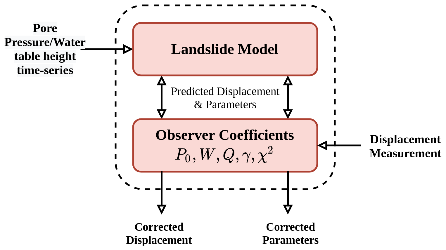
To summarize, the sensitivity to initial conditions and parameters is generally handled by simulating a model iteratively and adjusting the parameter values to obtain consistency with measured data (iterative approach). Alternatively, another efficient approach can be to run a model over time and continually fine-tune the parameters to synchronize with measured data, as in the so-called Kalman filter (or “observer”) approach (Kalman, 1960) (continuous approach). This second approach is much less common in landslide studies (see e.g. Lu and Zeng, 2020; Acar et al., 2008) and has seldom be used in conjunction with a mechanics-based model. In former studies, we applied both of these approaches to a landslide sliding consolidation model, using synthetically generated data: see Mishra et al. (2020a) for the iterative scheme (adjoint method), and Mishra et al. (2020b) for the continuous scheme (observer design). We found that a continuous scheme can be more suitable for reconstructing time-varying parameters. In addition, Kalman approach has the advantage of providing an optimal filtering solution whenever the model is linear and subject to additive white noises (Anderson and Moore, 1979). When used with a physical model, it shows powerful prediction capabilities thanks to the feedback connection with real data. Lastly, it also offers tuning parameters to act on the filtering $/$ reconstruction performances.

The present paper proposes to investigate further the use of a Kalman approach combined to a mechanical model for landslide monitoring, focusing on the problem of reconstruction of displacement patterns jointly with unknown parameters. As in our previous studies, a simple sliding block model with a limited number of parameters is considered for the sake of illustration. Notice that as a counterpart of the tuning possibilities offered by the Kalman approach, selecting appropriate tuning coefficient may actually prove difficult. In addition, it is known that Kalman approach can be hindered in the presence of nonlinearities in the model, which is a priori the case for the model considered here. Finally, one may have to face unexpected issues when moving from a methodological approach to its actual implementation with real data. In this context, the main contributions of this work are the following: (1) Regarding the model, it is first shown how a linear representation can be derived from the original nonlinear formulation, making the problem amenable to a Kalman approach. (2) Regarding the tuning, the use of an exponential forgetting factor is proposed in the chosen discrete-time observer approach (Ţiclea and Besançon, 2013, 2009) to improve reconstruction performances. An original resetting method is introduced in the observer for a better convergence of the estimates. Furthermore, a novel iterative approach for tuning observer coefficients is proposed, considering both real and synthetic test cases. (3) Finally, regarding implementation, it should be emphasized that this study is based on monitoring data (displacement and water table height) measured on a real landslide (Bernardie et al., 2014), and that promising applications to landslide forecasting are also demonstrated.

Since the main objective of this paper is to present the methodology and illustrate its potential on real data, the work relies – as in our previous studies – on a simplified physically-based landslide model depicting block sliding behavior with a predefined slip surface. A viscoplastic sliding resistance law is assumed (Herrera et al., 2013). Although extremely simplified, such a 1D approach can provide a first approximation of landslide motion. The targeted applications concern slow-moving landslides whose dynamics is primarily controlled by water table fluctuations. In addition, we assume that water table height is known, and focus on the reconstruction of landslide displacement and mechanical parameters at a single location. Extension of the approach to fully coupled hydromechanical models and/or more complex 2D or 3D mobility models (Chae et al., 2017) shall be considered in future work, but will require more extensive spatial datasets for estimation and prediction purposes.

The structure of the paper is as follows: The simplified viscoplastic sliding model is introduced in Sect. 2, together with the corresponding estimation problem. Section 3 presents the proposed reconstruction scheme. In Sect. 4, simulation results illustrate the effectiveness of the estimation scheme on the considered test case, namely Super-Sauze landslide (French Alps). Section 5 extends the proposed observer to the purpose of landslide displacement forecasting, assuming that future water table height variations are known. Finally, Sect. 6 provides a conclusion and discusses future directions of the work.

2 Simplified landslide viscoplastic sliding model

The viscoplastic sliding model (Bernardie et al., 2014; Herrera et al., 2013; Corominas et al., 2005) represents the dynamics of the landslide as that of a rigid sliding block overlying a thin shear zone, as shown in Fig. 1.

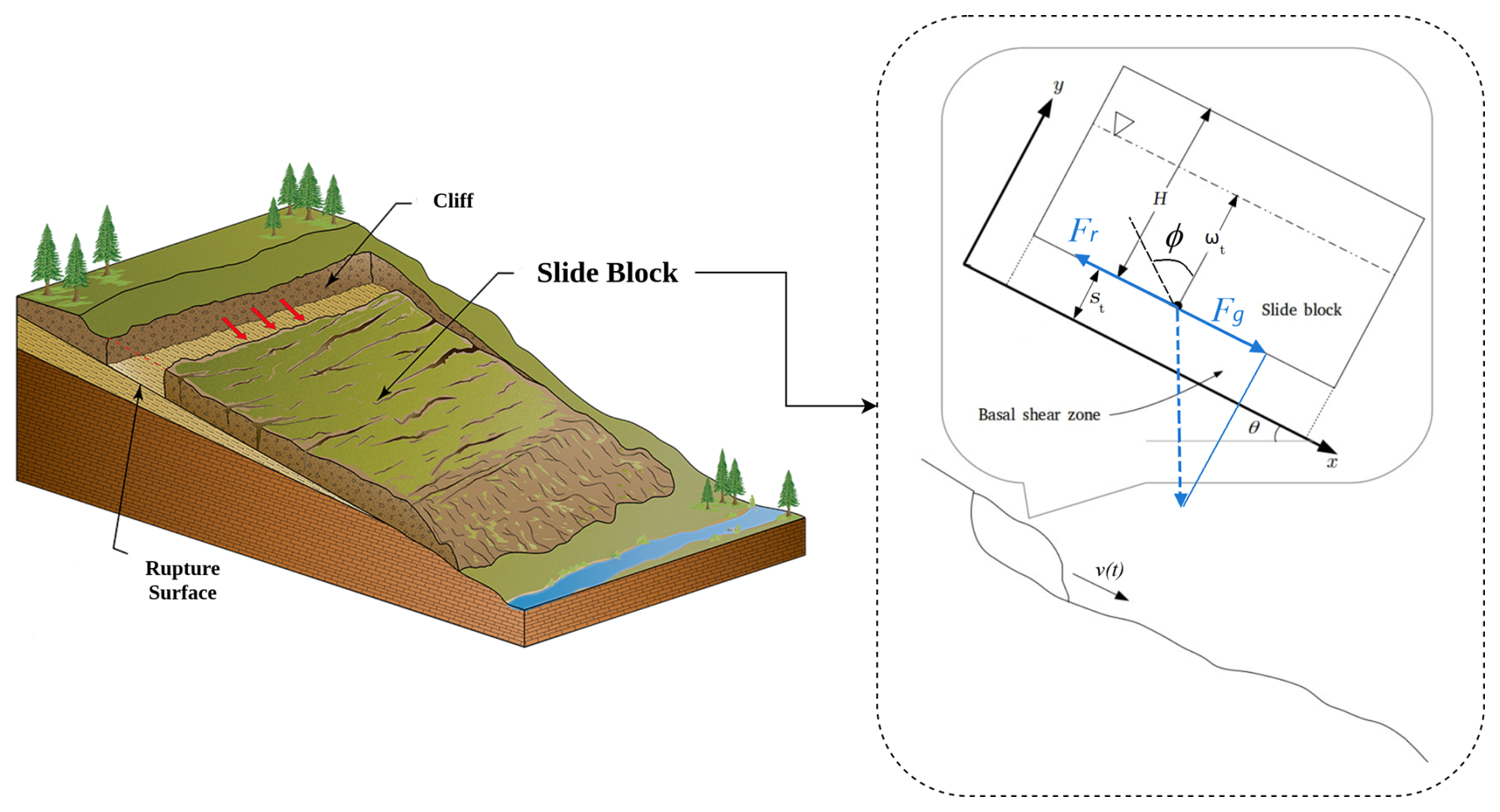
Figure 1 Schematic representation illustrating geometrical and mechanical variables used to model slide block motion: F_r resisting force; F_g driving gravity force; H block height; w_t water table height; s_t shear zone thickness; ϕ friction angle; θ inclination angle; v velocity [left picture is taken from Wyoming State Geological Survey website https://main.wsgs.wyo.gov/hazards/landslides/types-of-landslides/translational (last access: 20 January 2026), Credit: Wyoming State Geological Survey].

The motion is controlled by difference between the driving force F_g due to gravity and resisting forces F_r due to effective friction, cohesion, and viscosity. Hence, net acceleration of the block a is given by

$$\begin{array}{}\text{(1)}& \begin{array}{rl}\mathit{\rho }Ha\left(t\right)& =\mathit{\rho }gH\sin \mathit{\theta }-\left[\mathit{\rho }gH\cos \mathit{\theta }\tan \mathit{\varphi }-p\left(t\right)\tan \mathit{\varphi }\right.\\ & \left.+C+\mathit{\eta }v\left(t\right)/s_{\mathrm{t}}\right]\end{array}\end{array}$$

where ρ is the soil density, H is the slide block height, g is the acceleration due to gravity, θ is the inclination angle, p(t) is the basal pore water pressure at time t, v(t) is velocity of the slide block, and s_t is the basal shear zone thickness. The three mechanical parameters ϕ, C and η denote the friction angle, the cohesion, and the viscosity of the shear zone material, respectively.

For slow-moving landslides, the inertia is expected to remain much smaller than the other terms in Eq. (1), namely ρHa≈0. Assuming also that groundwater flow is parallel to the slope surface, the pore water pressure can be expressed as (Bernardie et al., 2014; Iverson, 2000)

$$\begin{array}{}\text{(2)}& p\left(t\right)={\mathit{\rho }}_{\mathrm{w}}g{\cos }^{\mathrm{2}}\mathit{\theta }{w}_{\mathrm{t}}\left(t\right)\end{array}$$

where ρ_w is the pore water density and w_t(t) is water table height, as shown in Fig. 1. Therefore, Eq. (1) can be rewritten as

$$\begin{array}{}\text{(3)}& \begin{array}{rl}\dot{d}=v\left(t\right)& ={\displaystyle \frac{s_{\mathrm{t}}}{\mathit{\eta }}}\left[\mathit{\rho }Hg\sin \mathit{\theta }-\mathit{\rho }\tan \mathit{\varphi }Hg\cos \mathit{\theta }\right.\\ & \left.-C+{\mathit{\rho }}_{\mathrm{w}}\tan \mathit{\varphi }g{\cos }^{\mathrm{2}}\mathit{\theta }{w}_{\mathrm{t}}\left(t\right)\right]\end{array}\end{array}$$

where d is the displacement of the slide block.

As upslope motion of the rigid slide block is physically impossible, the landslide velocity can not be negative. Such a situation arises whenever water table height w_t(t) goes below a critical water table height $w_{\mathrm{t}}^{\mathrm{crit}}$. From Eq. (3) the value of $w_{\mathrm{t}}^{\mathrm{crit}}$ is given by

$$\begin{array}{}\text{(4)}& w_{\mathrm{t}}^{\mathrm{crit}}={\displaystyle \frac{C-\mathit{\rho }Hg\sin \mathit{\theta }+\mathit{\rho }Hg\cos \mathit{\theta }\tan \mathit{\varphi }}{{\mathit{\rho }}_{\mathrm{w}}g{\cos }^{\mathrm{2}}\mathit{\theta }\tan \mathit{\varphi }}}.\end{array}$$

When $w_{\mathrm{t}}\left(t\right)\le w_{\mathrm{t}}^{\mathrm{crit}}$, landslide dynamics thus reduces to $\dot{d}=v\left(t\right)=\mathrm{0}$.

For known parameter values and water-table height (or pore water pressure), time series of displacement can be computed using Eq. (3) for $w_{\mathrm{t}}>w_{\mathrm{t}}^{\mathrm{crit}}$ and the above reduced dynamics otherwise. However, some material properties of the landslide (notably friction angle, cohesion and viscosity) are generally unknown, and therefore need to be estimated. In this paper, an observer-based approach is proposed to estimate friction angle ϕ, and viscosity η from measured displacement d_mea(t) and water table height w_t(t) time series, assuming cohesion C is known.

3 Reconstruction scheme

3.1 Observer-oriented representation

To address the observer problem, let us first normalize the unknown parameter η by introducing a typical viscosity scale $\stackrel{\mathrm{‾}}{\mathit{\eta }}$ in Eq. (3) as follows:

$$\begin{array}{}\text{(5)}& \begin{array}{rl}\stackrel{\mathrm{‾}}{\mathit{\eta }}\dot{d}& =\left({\displaystyle \frac{\stackrel{\mathrm{‾}}{\mathit{\eta }}}{\mathit{\eta }}}\right)s_{\mathrm{t}}\mathit{\rho }Hg\sin \mathit{\theta }-\left({\displaystyle \frac{\stackrel{\mathrm{‾}}{\mathit{\eta }}\tan \mathit{\varphi }}{\mathit{\eta }}}\right)s_{\mathrm{t}}\mathit{\rho }Hg\cos \mathit{\theta }\\ & -\left({\displaystyle \frac{\stackrel{\mathrm{‾}}{\mathit{\eta }}}{\mathit{\eta }}}\right)s_{\mathrm{t}}C+\left({\displaystyle \frac{\stackrel{\mathrm{‾}}{\mathit{\eta }}\tan \mathit{\varphi }}{\mathit{\eta }}}\right)s_{\mathrm{t}}{\mathit{\rho }}_{\mathrm{w}}g{\cos }^{\mathrm{2}}\mathit{\theta }{w}_{\mathrm{t}}\left(t\right).\end{array}\end{array}$$

This normalization is introduced to bring all parameters of interest in the same order of magnitude, as friction angle ϕ is dimensionless and usually comprised between 0 and 1.

Further, $\mathit{\eta }/\stackrel{\mathrm{‾}}{\mathit{\eta }}$ and ϕ being now the parameters to be estimated, let us define:

$$\begin{array}{}\text{(6)}& \left[\begin{array}{c}{\mathit{\theta }}_{\mathrm{1}}\\ {\mathit{\theta }}_{\mathrm{2}}\end{array}\right]:=s_{\mathrm{t}}\left[\begin{array}{cc}\mathit{\rho }Hg\sin \mathit{\theta }-C& -\mathit{\rho }Hg\cos \mathit{\theta }\\ \mathrm{0}& {\mathit{\rho }}_{\mathrm{w}}g{\cos }^{\mathrm{2}}\mathit{\theta }\end{array}\right]\left[\begin{array}{c}\stackrel{\mathrm{‾}}{\mathit{\eta }}/\mathit{\eta }\\ \stackrel{\mathrm{‾}}{\mathit{\eta }}\tan \mathit{\varphi }/\mathit{\eta }\end{array}\right].\end{array}$$

This substitution linearizes the model equation, making it more suitable for observer design. In order to estimate parameters, and assuming that those parameters vary slowly, the model can be extended by two additional differential equations, namely ${\dot{\mathit{\theta }}}_{\mathrm{1}}=\mathrm{0},{\dot{\mathit{\theta }}}_{\mathrm{2}}=\mathrm{0}$. Substituting Eq. (6) into (5), and taking the expression of $w_{\mathrm{t}}^{\mathrm{crit}}$ into account, the system equations finally become:

$$\begin{array}{}\text{(7)}& \begin{array}{rl}\dot{d}& =\left\{\begin{array}{ll}\frac{{\mathit{\theta }}_{\mathrm{1}}}{\stackrel{\mathrm{‾}}{\mathit{\eta }}}+\frac{{\mathit{\theta }}_{\mathrm{2}}}{\stackrel{\mathrm{‾}}{\mathit{\eta }}}{w}_{\mathrm{t}}\left(t\right)& \text{if }{w}_{\mathrm{t}}\left(t\right)>w_{\mathrm{t}}^{\mathrm{crit}}\\ \mathrm{0}& \text{otherwise}\end{array}\right.\\ {\dot{\mathit{\theta }}}_{\mathrm{1}}& =\mathrm{0},{\dot{\mathit{\theta }}}_{\mathrm{2}}=\mathrm{0}.\end{array}\end{array}$$

3.2 Discrete-time model

Instruments used for landslide monitoring collect data with a particular time resolution, e.g., hourly. Therefore, to adapt with discrete measurements (at times denoted by t^k), let us express the system dynamics in discrete time as follows

$$\begin{array}{}\text{(8)}& \stackrel{{\mathit{x}}^{k+\mathrm{1}}}{\overbrace{\left[\begin{array}{c}{d}^{k+\mathrm{1}}\\ {\mathit{\theta }}_{\mathrm{1}}^{k+\mathrm{1}}\\ {\mathit{\theta }}_{\mathrm{2}}^{k+\mathrm{1}}\end{array}\right]}}=\left\{\begin{array}{ll}\stackrel{{\stackrel{\mathrm{‾}}{\mathbf{A}}}_{\mathrm{1}}^k}{\overbrace{\left[\begin{array}{ccc}\mathrm{1}& \frac{\mathrm{d}t}{\stackrel{\mathrm{‾}}{\mathit{\eta }}}& \frac{\mathrm{d}t}{\stackrel{\mathrm{‾}}{\mathit{\eta }}}{w}_{\mathrm{t}}^k\\ \mathrm{0}& \mathrm{1}& \mathrm{0}\\ \mathrm{0}& \mathrm{0}& \mathrm{1}\end{array}\right]}}\stackrel{{\mathit{x}}^k}{\overbrace{\left[\begin{array}{c}{d}^k\\ {\mathit{\theta }}_{\mathrm{1}}^k\\ {\mathit{\theta }}_{\mathrm{2}}^k\end{array}\right]}},& \text{if }{w}_{\mathrm{t}}^k>w_{\mathrm{t}}^{\mathrm{crit}}\\ & \\ \underset{{\stackrel{\mathrm{‾}}{\mathbf{A}}}_{\mathrm{2}}^k}{\underbrace{\left[\begin{array}{ccc}\mathrm{1}& \mathrm{0}& \mathrm{0}\\ \mathrm{0}& \mathrm{1}& \mathrm{0}\\ \mathrm{0}& \mathrm{0}& \mathrm{1}\end{array}\right]}}\underset{{\mathit{x}}^k}{\underbrace{\left[\begin{array}{c}{d}^k\\ {\mathit{\theta }}_{\mathrm{1}}^k\\ {\mathit{\theta }}_{\mathrm{2}}^k\end{array}\right]}}& \text{otherwise}\end{array}\right.\end{array}$$

where d$t=t^{k+\mathrm{1}}-t^k$ is the discrete-time step, and x^k gathers all system variables. The measurement model is given as

$$\begin{array}{}\text{(9)}& y^k=d_{\mathrm{mea}}^k=\stackrel{\stackrel{\mathrm{‾}}{\mathbf{C}}}{\overbrace{\left[\begin{array}{ccc}\mathrm{1}& \mathrm{0}& \mathrm{0}\end{array}\right]}}\stackrel{{\mathit{x}}^k}{\overbrace{\left[\begin{array}{c}{d}^k\\ {\mathit{\theta }}_{\mathrm{1}}^k\\ {\mathit{\theta }}_{\mathrm{2}}^k\end{array}\right]}}+r^k\end{array}$$

where y^k denotes the actually available measurement, and r^k some measurement noise.

3.3 Discrete-time exponential forgetting factor observer

Discrete-time exponential forgetting factor observer (or Kalman filtering with forgetting factor) provides least mean-square estimate with an added feature of giving more weight to the most recent measurements. If γ denotes the forgetting factor and ${\widehat{x}}_{\mathrm{0}}$ denotes the initial guess for x^k, the approach optimizes the following objective function:

$$\begin{array}{}\text{(10)}& \begin{array}{rl}{J}_k\left({\widehat{\mathit{x}}}_{\mathrm{0}}^k\right)& ={\mathit{\gamma }}^k{\left({\widehat{\mathit{x}}}_{\mathrm{0}}^k-{\widehat{\mathit{x}}}_{\mathrm{0}}\right)}^T{\mathbf{P}}_{\mathrm{0}}^{-\mathrm{1}}\left({\widehat{\mathit{x}}}_{\mathrm{0}}^k-{\widehat{\mathit{x}}}_{\mathrm{0}}\right)\\ & +\sum _{l=\mathrm{0}}^k{\mathit{\gamma }}^{k-l}{\left({\widehat{y}}^l-y^l\right)}^T{W}^{-\mathrm{1}}\left({\widehat{y}}^l-y^l\right)\end{array}\end{array}$$

subject to system dynamics

$$\begin{array}{}\text{(11)}& \begin{array}{rl}{\widehat{\mathit{x}}}^{k+\mathrm{1}}& ={\stackrel{\mathrm{‾}}{\mathbf{A}}}^k{\widehat{\mathit{x}}}^k\\ {\widehat{y}}^k& =\stackrel{\mathrm{‾}}{\mathbf{C}}{\widehat{\mathit{x}}}^k\end{array}\end{array}$$

as constraints, with $\mathit{\gamma }\in (\mathrm{0},\mathrm{1}),{\mathbf{P}}_{\mathrm{0}}={\mathbf{P}}_{\mathrm{0}}^T>\mathrm{0},W=W^T>\mathrm{0}$. The solution of this optimization problem (Ţiclea and Besançon, 2013) is provided through measurement update equations:

$$\begin{array}{}\text{(12)}& {\widehat{\mathit{x}}}_{\mathrm{c}}^k={\widehat{\mathit{x}}}_{\mathrm{p}}^k-{\mathit{K}}^k\left(\stackrel{\mathrm{‾}}{\mathbf{C}}{\widehat{\mathit{x}}}_{\mathrm{p}}^k-y^k\right),\end{array}$$

with

$$\begin{array}{}\text{(13)}& {\mathit{K}}^k={\mathbf{P}}^k{\stackrel{\mathrm{‾}}{\mathbf{C}}}^T{\left(\stackrel{\mathrm{‾}}{\mathbf{C}}{\mathbf{P}}_{\mathrm{p}}^k{\stackrel{\mathrm{‾}}{\mathbf{C}}}^T+W\right)}^{-\mathrm{1}},\end{array}$$

and time update equations,

$$\begin{array}{}\text{(14)}& {\widehat{\mathit{x}}}_{\mathrm{p}}^{k+\mathrm{1}}={\stackrel{\mathrm{‾}}{\mathbf{A}}}^k{\widehat{\mathit{x}}}_{\mathrm{c}}^k\end{array}$$

$$\begin{array}{}\text{(15)}& {\mathbf{P}}^{k+\mathrm{1}}={\mathit{\gamma }}^{-\mathrm{1}}{\stackrel{\mathrm{‾}}{\mathbf{A}}}^k\left[\mathbf{I}-{\mathit{K}}^k\stackrel{\mathrm{‾}}{\mathbf{C}}\right]{\mathbf{P}}^k{\stackrel{\mathrm{‾}}{\mathbf{A}}}^{k^T}+\mathbf{Q}\end{array}$$

with initialization P₀. Here K^k is the Kalman gain, P is the auto-covariance of state estimation error, W is the auto-covariance of measurement noise r, $\mathit{\gamma }\in (\mathrm{0},\mathrm{1})$ is the forgetting factor, and Q is the process noise auto-covariance matrix.

For dynamics (Eqs. 8–9), observer Eqs. (12)–(15) provides estimates of $\widehat{d}$, ${\widehat{\mathit{\theta }}}_{\mathrm{1}}$ and ${\widehat{\mathit{\theta }}}_{\mathrm{2}}$. Based on these estimates at each time step, firstly $\stackrel{\mathrm{‾}}{\mathit{\eta }}/\widehat{\mathit{\eta }}$ and $\stackrel{\mathrm{‾}}{\mathit{\eta }}\tan \widehat{\mathit{\varphi }}/\widehat{\mathit{\eta }}$ are reconstructed using Eq. (6):

$$\begin{array}{}\text{(16)}& \left[\begin{array}{c}\stackrel{\mathrm{‾}}{\mathit{\eta }}/\widehat{\mathit{\eta }}\\ \stackrel{\mathrm{‾}}{\mathit{\eta }}\tan \widehat{\mathit{\varphi }}/\widehat{\mathit{\eta }}\end{array}\right]={\displaystyle \frac{\mathrm{1}}{s_{\mathrm{t}}}}{\left[\begin{array}{cc}\mathit{\rho }Hg\sin \mathit{\theta }-C& -\mathit{\rho }Hg\cos \mathit{\theta }\\ \mathrm{0}& {\mathit{\rho }}_{\mathrm{w}}g{\cos }^{\mathrm{2}}\mathit{\theta }\end{array}\right]}^{-\mathrm{1}}\left[\begin{array}{c}{\widehat{\mathit{\theta }}}_{\mathrm{1}}\\ {\widehat{\mathit{\theta }}}_{\mathrm{2}}\end{array}\right],\end{array}$$

followed by

$$\begin{array}{}\text{(17)}& \widehat{\mathit{\eta }}={\displaystyle \frac{\stackrel{\mathrm{‾}}{\mathit{\eta }}}{\left[\stackrel{\mathrm{‾}}{\mathit{\eta }}/\widehat{\mathit{\eta }}\right]}}\mathit{\&}\widehat{\mathit{\varphi }}={\tan }^{-\mathrm{1}}\left(\left[\stackrel{\mathrm{‾}}{\mathit{\eta }}\tan \widehat{\mathit{\varphi }}/\widehat{\mathit{\eta }}\right]{\displaystyle \frac{\widehat{\mathit{\eta }}}{\stackrel{\mathrm{‾}}{\mathit{\eta }}}}\right).\end{array}$$

In the proposed estimation scheme, $w_{\mathrm{t}}^{\mathrm{crit}}$ plays an important role. This quantity itself depends on the parameter values, therefore at each step it is estimated using Eq. (4).

3.4 State estimation error covariance matrix P resetting

In the design presented so far, unknown parameters are assumed to be constant or slowly varying. However, in practical applications, these parameters may also be subject to abrupt changes. In order to handle such situations, a resetting of state estimation error covariance matrix P is proposed here. In order to detect abrupt variations, the Mahalanobis distance (Gnanadesikan and Kettenring, 1972) between actual and predicted measurements for some previous times (t^k−m to t^k), with more weight on the most recent times, is calculated as:

$$\begin{array}{}\text{(18)}& D^k=\sum _{j=k-m}^k{\mathit{\gamma }}^{k-j}({\mathbf{C}}^j{\widehat{\mathit{x}}}^j-y^j{)}^T{W}^{-\mathrm{1}}({\mathbf{C}}^j{\widehat{\mathit{x}}}^j-y^j).\end{array}$$

At times for which D^k exceeds a given threshold (D^k>χ²), P^k is reset to P₀. This threshold can be obtained from the chi-square table (Pearson, 1900) according to the confidence level of the measurement system. For example, when confidence level is 99 % and the dimension of the measurement system vector is 1, the corresponding chi-square value is χ²=6.635. Note that there is a possibility of multiple successive resettings, which could hamper the overall performance of the estimation scheme. Such a scenario is avoided by forbidding resetting for some short duration (e.g., m instances) after each detected resetting.

3.5 Observer coefficients tuning

Observer coefficients $({\mathbf{P}}_{\mathrm{0}},W,\mathbf{Q},\mathit{\gamma },{\mathit{\chi }}^{\mathrm{2}},m)$ should be properly chosen to recover model information (see Fig. 2). In usual applications, these coefficients are manually tuned until proper convergence in estimates are obtained. However, such applications require some nominal values of the parameters being known (e.g. Ţiclea and Besançon, 2009), which is not the case in the present study. Therefore, a novel approach is introduced, which considers both synthetic and actual data cases to verify the estimates, according to the methodology summarized in Fig. 3.

Figure 2 Principle of discrete-time exponential forgetting factor observer.

Figure 3 Observer coefficients tuning methodology.

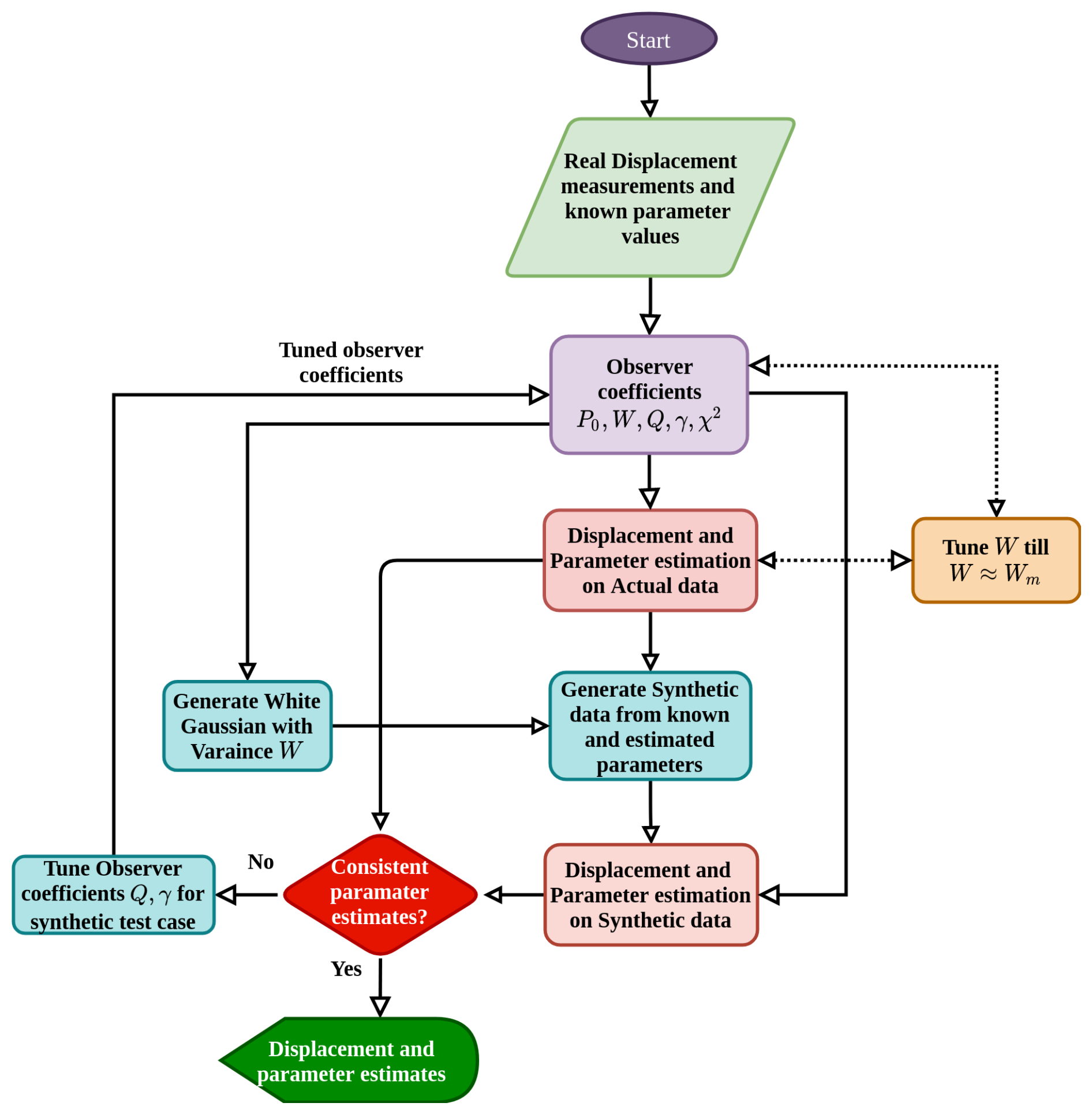
In this approach, given an assumed confidence level in the measurement model and a known dimension of the measurement vector, the value of χ² is fixed throughout the tuning process. Along with χ², P₀ and m are also fixed. The matrix P₀ is obtained from its definition with guessed initial states ${\widehat{\mathit{x}}}_{\mathrm{0}}$. The coefficient m is guessed from some rough initial simulation results on synthetic test cases and can be chosen from the time steps required for first convergence. Once filter coefficients χ²,P₀ and m are fixed, the estimation scheme is applied on real measurements with some initial values of Q, γ and W. For the actual data case, W is manually tuned until W≈W_m where, W_m is the variance of signal $d_{\mathrm{mea}}-\widehat{d}$. Then synthetic measurements are generated by solving Eq. (3) using water table height measurements and estimated parameters (smoothed estimated viscosity and averaged estimated frictional angle) from an actual data case. Now estimation scheme is employed on these synthetic measurements keeping filter coefficients W, γ, and Q identical as in the actual case. If estimated parameters from both actual case and synthetic test are consistent, filter coefficients tuning process can be stopped; else γ and Q are adjusted with the help of quantitative indicator I_q given as

$$\begin{array}{}\text{(19)}& I_q=\sum _{k=\mathrm{1}}^n\left|{\displaystyle \frac{q^k-{\widehat{q}}^k}{q^k}}\right|\end{array}$$

where q^k is the parameter of interest (viscosity and friction angle) at time k and ${\widehat{q}}^k$ is the corresponding estimated parameter. Indicator I_q provides information on how close the estimated parameters are to the parameters used to generate the synthetic test case. The above process of tuning W from actual case, followed by tuning γ and Q on synthetic test cases, is continued until parameter estimates in both cases are consistent to each other, as shown in Fig. 3.

4 Estimation results

4.1 Super-Sauze landslide data

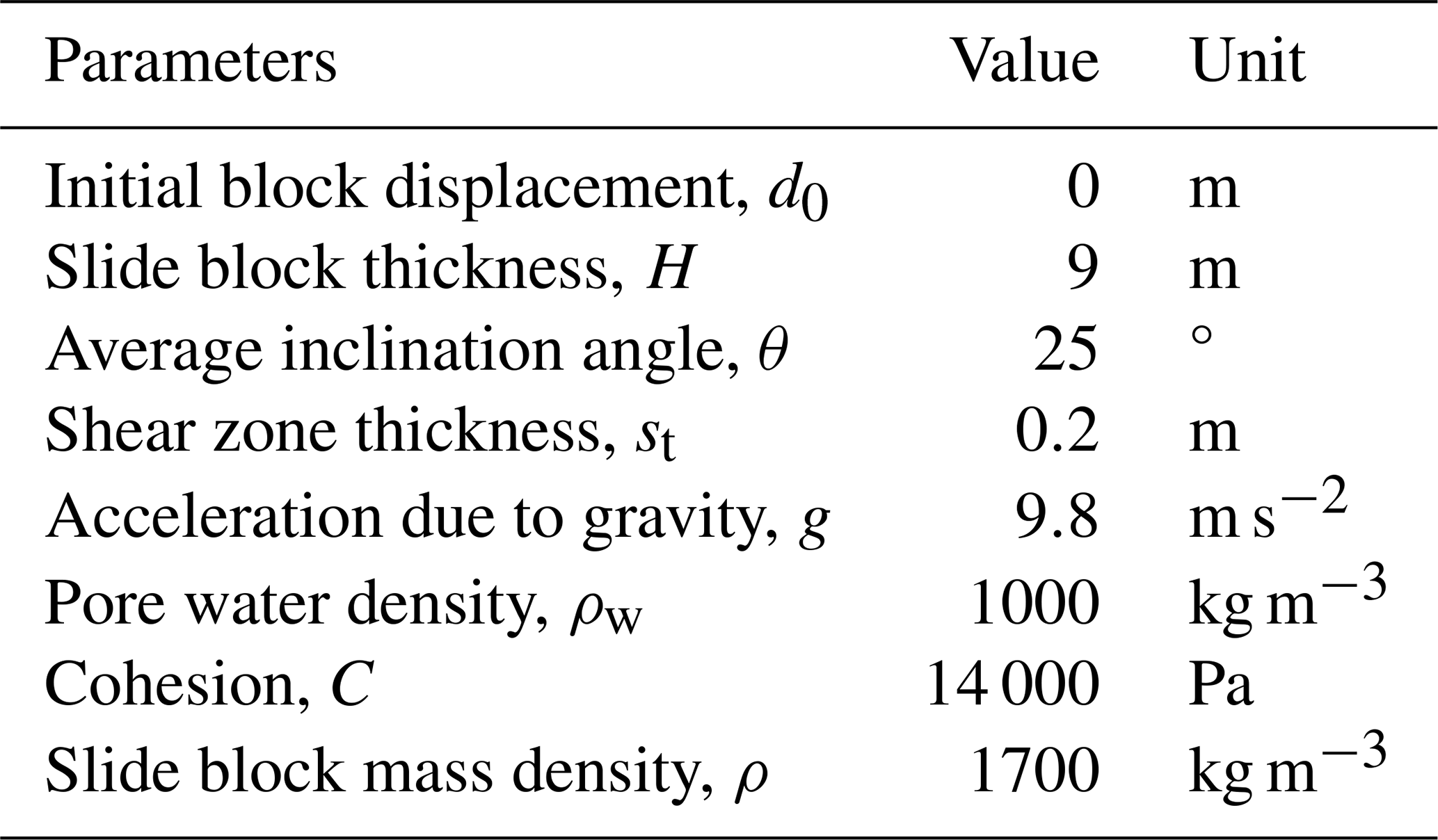
The Super-Sauze landslide is a slow-moving earthflow located in the southern French Alps which is monitored by the French Multi-disciplinary Observatory OMIV for meteorological parameters, slope hydrology and slope kinematics. Detailed descriptions of this landslide and of the monitoring system can be found in previous studies (Bernardie et al., 2014; Travelletti and Malet, 2012; Malet et al., 2005). It should be mentioned that the landslide, whose volume is estimated around 560 000 m³, is characterized by a spatially heterogeneous displacement pattern with average velocities varying between 0.001 and 0.03 m d⁻¹ (Bernardie et al., 2014). Clearly, the simple slide block model used in this study cannot aim to reproduce this complex process. However, in line with model assumptions, displacements are mainly parallel to the dip direction of slope. The landslide is characterized by two vertical units, with a slip surface in between. Velocities appear to be mainly controlled by evolutions of the water table level, with accelerations up to 0.4 m d⁻¹ typically observed during spring. We thus take advantage of the rich dataset available in this site to illustrate the proposed estimation methodology and show the robustness of the approach, focusing on one specific monitoring location.

Specifically, the observer approach is applied to displacement $d_{\mathrm{mea}}^k$ and pore water pressure p^k time-series for a period of high water table level and accelerated motion from 7 to 23 May 1999 (16 d) (Bernardie et al., 2014). We hypothesize that the simple model considered in this study is sufficient to reproduce this acceleration phase. The data, acquired with a time resolution dt=2.4 h (8640 s), correspond to one of the most active parts of the landslide [location B₂ in Fig. 4 of Bernardie et al., 2014]. Displacement and pore water pressure are measured by a wire extensometer and piezometer, respectively. The piezometer is located at −4 m depth, while the slip surface is at a depth of −9 m. In the proposed scheme, a water table height time-series $w_{\mathrm{t}}^k$ is required as an input. Water-table height is reconstructed from pore pressure p^k using assumption of groundwater flow parallel to the slope surface (Eq. 2): $w_{\mathrm{t}}^k=\mathrm{5}+p^k/\left({\mathit{\rho }}_{\mathrm{w}}g{\cos }^{\mathrm{2}}\mathit{\theta }\right)$. The reconstructed water-table height time-series along with the measured displacement are shown in Fig. 4. Known parameter values are indicated in Table 1. The value of density ρ=1700 kg m⁻³ is chosen to correspond to saturated soil density as the water table height is close to full saturation level (Fig. 4).

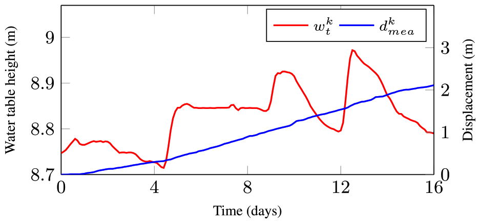
Figure 4 Super-Sauze landslide data from 7 to 23 May 1999: Displacement measurement $d_{\mathrm{mea}}^k$ and reconstructed water table height time-series $w_{\mathrm{t}}^k$ obtained from Bernardie et al. (2014) (notice that w_t is referenced to the base of the sliding block, thus $w_{\mathrm{t}}^k\le \mathrm{9}$ m).

Table 1 Known geometrical and material parameter values.

4.2 Observer results

Displacement pattern $\widehat{d}$ along with unknown soil properties ($\widehat{\mathit{\eta }}$, $\widehat{\mathit{\varphi }}$) are reconstructed with the help of the proposed estimation scheme (see Sect. 3), for known parameter values (Table 1), displacement measurements and water table height time-series (Fig. 4). As mentioned in Sect. 3.5, for an assumed confidence level of 99 % on measurements with a dimension equal to 1, the value of χ² is set to 6.635. The value of m is fixed to 5 (see Sect. 3.5). Initial auto-covariance of state estimation error P₀ is defined as the variance of ${\mathit{x}}_{\mathrm{0}}-{\widehat{\mathit{x}}}_{\mathrm{0}}$, where, ${\mathit{x}}_{\mathrm{0}}={\left[\begin{array}{ccc}{d}_{\mathrm{0}}& {\mathit{\theta }}_{{\mathrm{1}}_{\mathrm{0}}}& {\mathit{\theta }}_{{\mathrm{2}}_{\mathrm{0}}}\end{array}\right]}^T$ (generally assumed to be a diagonal matrix). Here, d₀ and ${\widehat{d}}_{\mathrm{0}}$ are equal to 0; therefore the first entry in P₀ is assumed equal to W, which represents the auto-covariance of measurement noise r. Further, since the actual values of θ₁ and θ₂ are not known, we assume initial errors of few percents of the expected values (order of magnitude), considering guesses on ${\widehat{\mathit{\theta }}}_{\mathrm{1}}$ and ${\widehat{\mathit{\theta }}}_{\mathrm{2}}$ calculated with Eq. (6) for assumed η₀ and ϕ₀ equal to 10⁸ Pa s and 35°, respectively. Finally, the matrix P₀ is thus set to

$$\begin{array}{}\text{(20)}& {\mathbf{P}}_{\mathrm{0}}=\left[\begin{array}{ccc}W& \mathrm{0}& \mathrm{0}\\ \mathrm{0}& \mathrm{10}\mathrm{000}& \mathrm{0}\\ \mathrm{0}& \mathrm{0}& \mathrm{100}\end{array}\right].\end{array}$$

For fixed observer coefficients χ², m and P₀, and starting from initial values γ=0.95, $W={\mathrm{10}}^{-\mathrm{12}}$, and $\mathbf{Q}={\mathrm{10}}^{-\mathrm{12}}{I}_{\mathrm{3}\times \mathrm{3}}$ (where I_3×3 is the identity matrix of dimension 3) for the other coefficients, the estimation scheme is applied on real measurements. Based on the actual Super-Sauze data, W is manually tuned until W≈W_m, where W_m is the variance of $d_{\mathrm{mea}}-\widehat{d}$. This condition gets satisfied for $W=\mathrm{7.7}\times {\mathrm{10}}^{-\mathrm{6}}$. For this set of observer coefficients $({\mathit{\chi }}^{\mathrm{2}},m,{\mathbf{P}}_{\mathrm{0}},\mathit{\gamma },W,\mathbf{Q})$, the obtained estimation results are shown in Fig. 5. It is observed that the friction angle $\widehat{\mathit{\varphi }}$ is almost constant, while the viscosity $\widehat{\mathit{\eta }}$ varies with time in correlation with water table height. Synthetic measurements are then generated based on an average value of $\widehat{\mathit{\varphi }}$ $\left({\widehat{\mathit{\varphi }}}_{\mathrm{avg}}\right)$ and a filtered viscosity time-series ${\widehat{\mathit{\eta }}}_{\mathrm{fil}}$ obtained by applying a Savitzky-Golay filter on $\widehat{\mathit{\eta }}$ (Sharifi et al., 2022; Savitzky and Golay, 1964) (Fig. 5). In the synthetically generated displacement, a random Gaussian noise with variance W is injected. Using those synthetically generated data, the estimation scheme is applied again with identical observer coefficients as in the actual case. Corresponding results can be seen in Fig. 6. It is observed that the parameter estimates are not converging to ${\widehat{\mathit{\varphi }}}_{\mathrm{avg}}$ and ${\widehat{\mathit{\eta }}}_{\mathrm{fil}}$ (Fig. 6a, b). Therefore, the values of γ and Q are adjusted with the help of the quantitative indicator I_η (see Eq. 19). Notice that the indicator I_η is found to be more sensitive to variations in observer coefficients than I_ϕ and I_d. This is explained by the fact that the friction angle is almost constant, while displacement is well estimated with measurement update Eq. (12) of the observer.

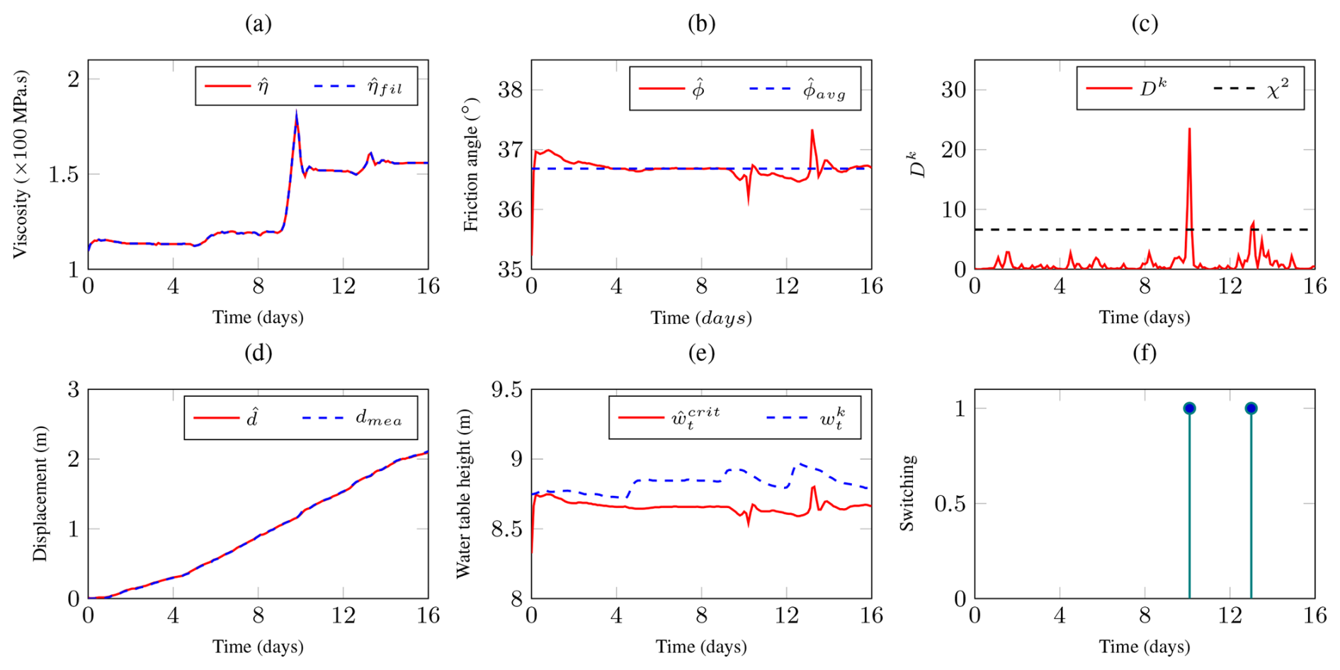
Figure 5 Initial estimation results for Super-Sauze case with real data and observer coefficient values γ=0.95, $W=\mathrm{7.7}\times {\mathrm{10}}^{-\mathrm{6}}$, $\mathbf{Q}={\mathrm{10}}^{-\mathrm{12}}{I}_{\mathrm{3}\times \mathrm{3}}$: (a)–(b) parameter estimates ($\widehat{\mathit{\eta }}$, $\widehat{\mathit{\varphi }}$), filtered viscosity ${\widehat{\mathit{\eta }}}_{\mathrm{fil}}$ and averaged friction angle ${\widehat{\mathit{\varphi }}}_{\mathrm{avg}}$, (c) Mahalanobis distance between estimated and measured displacement D^k, (d) displacement estimate $\widehat{d}$ and displacement measurement d_mea, (e) critical water table height estimate ${\widehat{w}}_{\mathrm{t}}^{\mathrm{crit}}$ and water table height measurement $w_{\mathrm{t}}^k$, (f) resetting times of the covariance matrix.

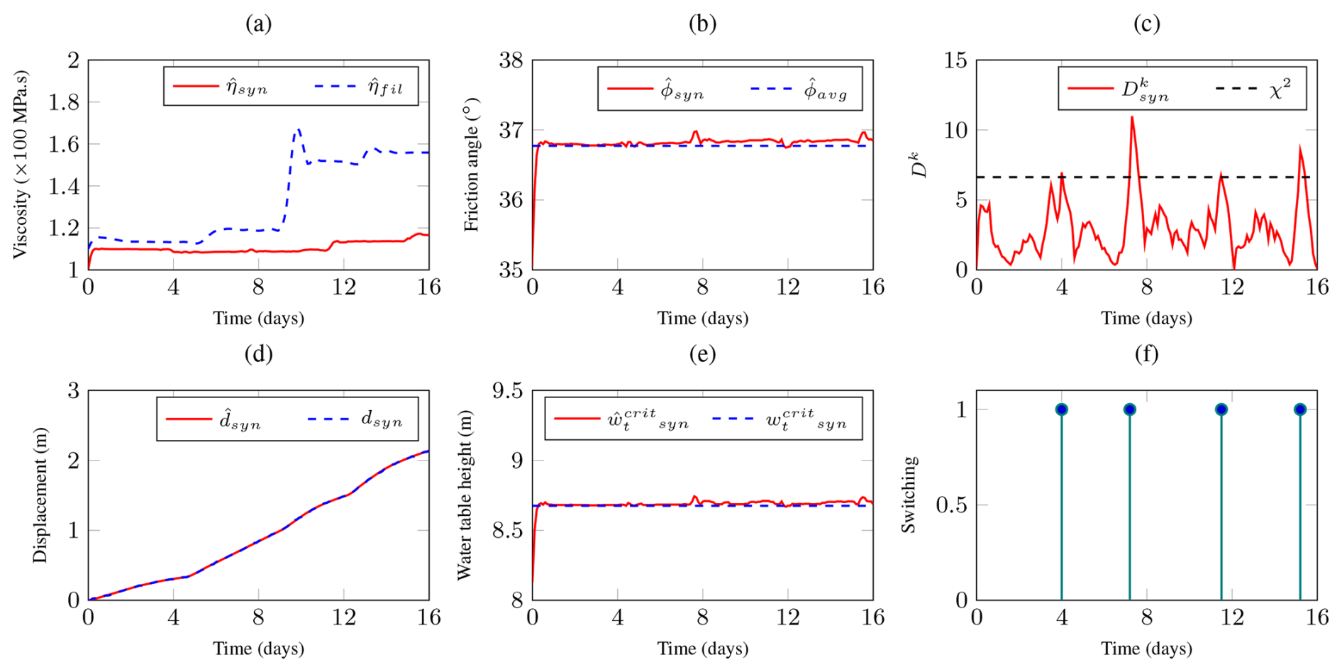
Figure 6 Initial estimation results for Super-Sauze synthetic test case with observer coefficient values γ=0.95, $W=\mathrm{7.7}\times {\mathrm{10}}^{-\mathrm{6}}$, $\mathbf{Q}={\mathrm{10}}^{-\mathrm{12}}{I}_{\mathrm{3}\times \mathrm{3}}$: (a)–(b) parameter estimates (${\widehat{\mathit{\eta }}}_{\mathrm{syn}}$, ${\widehat{\mathit{\varphi }}}_{\mathrm{syn}}$), (c) Mahalanobis distance between estimated and synthetic displacement $D_{\mathrm{syn}}^k$, (d) displacement estimate ${\widehat{d}}_{\mathrm{syn}}$ and synthetic displacement measurement d_syn, (e) critical water table height estimate ${{\widehat{w}}_{\mathrm{t}}^{\mathrm{crit}}}_{\mathrm{syn}}$, (f) resetting times of the covariance matrix.

Table 2 Sensitivity analysis for tuning observer coefficients γ and Q based on Super-Sauze synthetic test case: values of indicator I_η (minimum value is highlighted in bold).

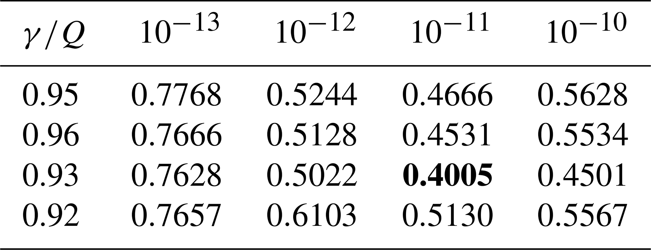
Based on the sensitivity analysis (Table 2), the minimum value I_η=0.4005 is obtained for γ=0.93 and $\mathbf{Q}={\mathrm{10}}^{-\mathrm{11}}{I}_{\mathrm{3}\times \mathrm{3}}$. Hence, values of γ and Q in the estimation scheme are updated accordingly, and new simulation results for synthetic and actual cases are computed. Still, obtained parameter estimates are not consistent. Therefore, the process of tuning W for the actual case with condition W≈W_m, and tuning γ and Q with the indicator for a synthetic test case, is continued. After 6 iterations, consistency in parameter estimates is obtained between the synthetic test case (Fig. 7a–b) and the actual case (Fig. 8a–b). In both cases, the average value of the estimated friction angle is found to be equal to 36.8°, while approximately similar variations in estimated viscosity are observed.

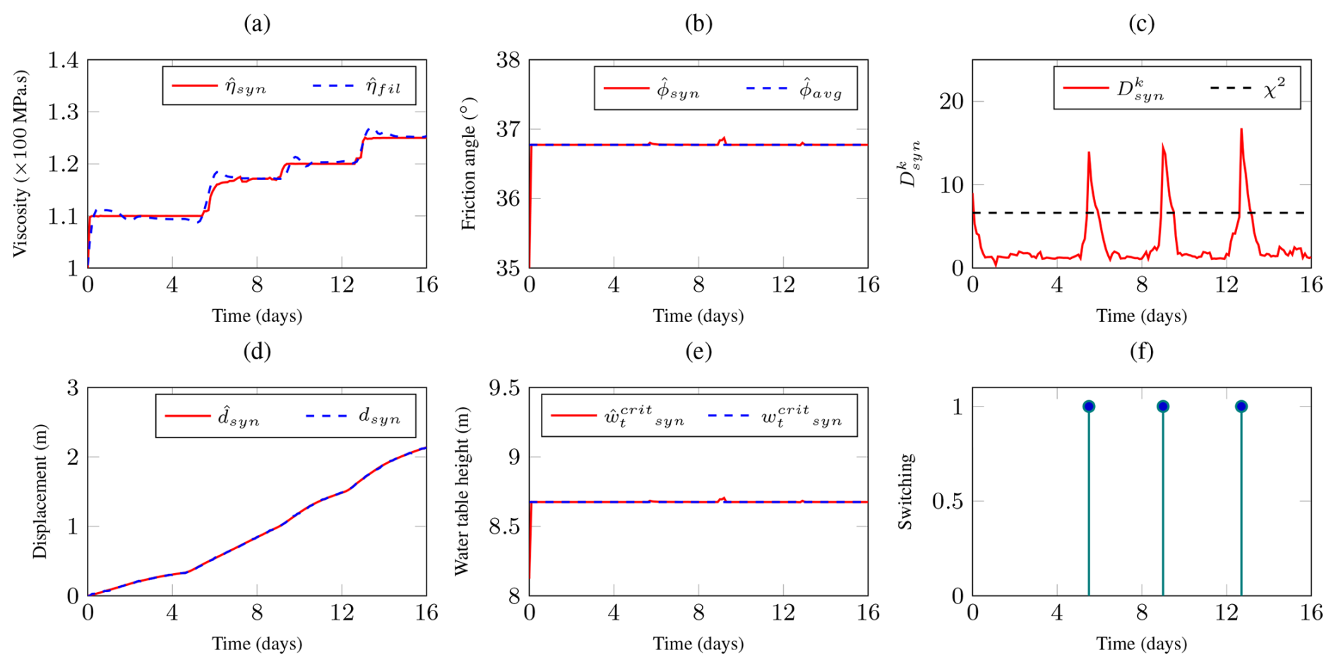
Figure 7 Final estimation results for Super-Sauze synthetic test case with observer coefficient values γ=0.9, $W=\mathrm{6}\times {\mathrm{10}}^{-\mathrm{5}}$, $\mathbf{Q}={\mathrm{10}}^{-\mathrm{11}}{I}_{\mathrm{3}\times \mathrm{3}}$: (a)–(b) parameter estimates (${\widehat{\mathit{\eta }}}_{\mathrm{syn}}$, ${\widehat{\mathit{\varphi }}}_{\mathrm{syn}}$), (c) Mahalanobis distance between estimated and synthetic displacement $D_{\mathrm{syn}}^k$, (d) displacement estimate ${\widehat{d}}_{\mathrm{syn}}$ and synthetic displacement measurement d_syn, (e) critical water table height estimate ${{\widehat{w}}_{\mathrm{t}}^{\mathrm{crit}}}_{\mathrm{syn}}$, (f) resetting times of the covariance matrix.

Notice that in the final results, water-table height always remains above critical water-table height ($w_{\mathrm{t}}^k>{\widehat{w}}_{\mathrm{t}}^{\mathrm{crit}}$), as shown in Fig. 8e. Resetting of the covariance matrix takes place when D^k>χ² as shown in Figs. 7c and 8c, and the corresponding times can be seen in Figs. 7f and 8f. Note that, as expected, these resetting times correspond to abrupt changes in viscosity.

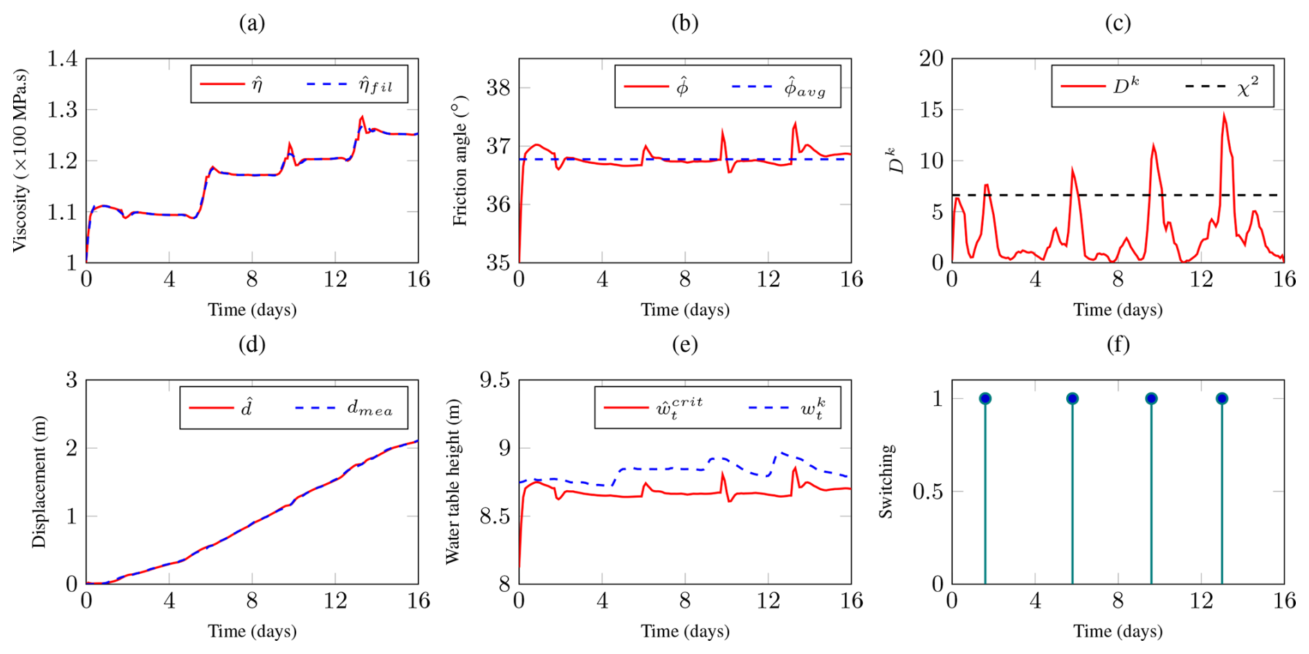
Figure 8 Final estimation results for Super-Sauze case with real data and observer coefficient values γ=0.9, $W=\mathrm{6}\times {\mathrm{10}}^{-\mathrm{5}}$, $\mathbf{Q}={\mathrm{10}}^{-\mathrm{11}}{I}_{\mathrm{3}\times \mathrm{3}}$: (a)–(b) parameter estimates ($\widehat{\mathit{\eta }}$, $\widehat{\mathit{\varphi }}$), filtered viscosity η_fil and averaged friction angle ϕ_avg, (c) Mahalanobis distance between estimated and measured displacement D^k, (d) displacement estimate $\widehat{d}$ and displacement measurement d_mea, (e) critical water table height estimate ${\widehat{w}}_{\mathrm{t}}^{\mathrm{crit}}$ and water table height measurement $w_{\mathrm{t}}^k$, (f) resetting times of the covariance matrix.

5 Landslide displacement forecasting

The reconstruction scheme (Sect. 3) is based on the principle of prediction (Eq. 14) followed by correction (Eq. 12) of the information of interest: At each time step “k”, information is predicted for the next time step “k+1” with the help of Eq. (8) and then corrected based on the measurement. This corrected information is then used to predict for the next time step, etc. In the present case, “information” refers to displacement and parameters, i.e., ${\widehat{\mathit{x}}}^k={\left[\begin{array}{ccc}{\widehat{d}}^k& {\widehat{\mathit{\theta }}}_{\mathrm{1}}^k& {\widehat{\mathit{\theta }}}_{\mathrm{2}}^k\end{array}\right]}^T$. Hence, inherently, the proposed scheme can predict information for the next time step only. However, with minor update in Eq. (14), the prediction horizon can be extended to L time steps on the basis of the following law:

$$\begin{array}{}\text{(21)}& {\stackrel{\mathrm{‾}}{\mathit{x}}}_{\mathrm{p}}^{k+l}=\left\{\begin{array}{ll}{\stackrel{\mathrm{‾}}{\mathbf{A}}}^k{\stackrel{\mathrm{‾}}{\mathit{x}}}_c^k& \text{for}l=\mathrm{1}\\ {\stackrel{\mathrm{‾}}{\mathbf{A}}}^k{\stackrel{\mathrm{‾}}{\mathit{x}}}_p^{k+l-\mathrm{1}}& \text{for}l=\mathrm{2}\text{to}L-\mathrm{1}\end{array}\right.\end{array}$$

Notice that in order to account for the critical water table height, when a displacement value computed by Eq. (21) is lower than the former one, displacement is frozen.

To validate this extension of the approach, let us again consider the 16-day Super-Sauze landslide data. The prediction step is initiated after day eight, assuming that water table height time-series is known and that, at each time step, corresponding displacement is being measured. Two different prediction horizons are considered, namely 1 d (L=10 as step size dt=2.4 h) and 2 d (L=20). In Fig. 9a–c, displacement and parameter forecasts until day 9 and day 10 are presented. As the dynamics of time-varying parameters are a priori unknown, in model equations (Eq. 7) these parameters are assumed constant, as clearly visible in Fig. 9b–c. As a consequence, it is observed that the forecast becomes rapidly less accurate as we move away from the actual time (Fig. 9a). Figure 9d–f present moving horizon (1 and 2 d) predictions, i.e., at instance k the forecasts for k+10 and k+20, respectively are shown. As time advances, the estimated parameters start varying based on displacement measurements and the measurement update equation of the observer (see Fig. 9e–f). Overall, predicted displacements appear to agree reasonably well with the estimate obtained in Sect. 4. However, as it could be expected, accuracy of the forecast reduces as the prediction horizon L is increased.

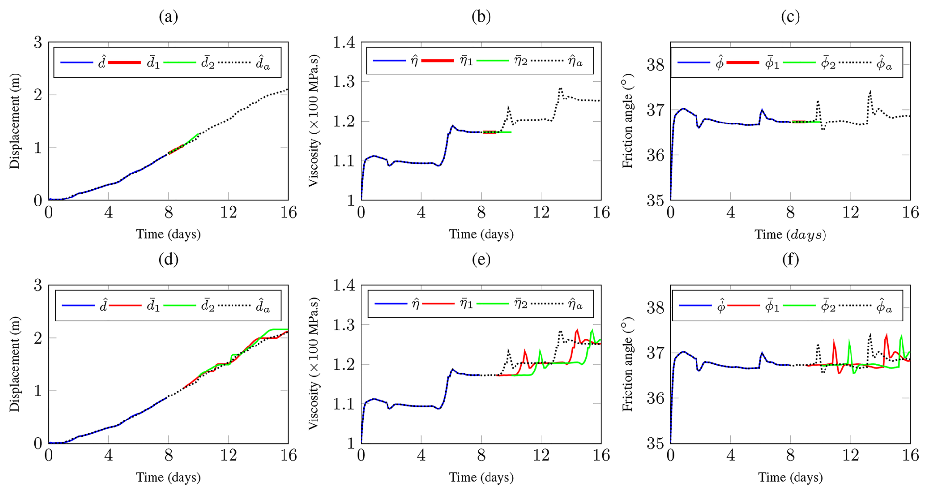
Figure 9 Landslide displacement [$\stackrel{\mathrm{‾}}{d}$] and unknown parameters [$\stackrel{\mathrm{‾}}{\mathit{\eta }},\stackrel{\mathrm{‾}}{\mathit{\varphi }}$] forecasting: (a)–(c) forecasts with prediction horizon 1 d [${\stackrel{\mathrm{‾}}{d}}_{\mathrm{1}},{\stackrel{\mathrm{‾}}{\mathit{\eta }}}_{\mathrm{1}},{\stackrel{\mathrm{‾}}{\mathit{\varphi }}}_{\mathrm{1}}$] and 2 d [${\stackrel{\mathrm{‾}}{d}}_{\mathrm{2}},{\stackrel{\mathrm{‾}}{\mathit{\eta }}}_{\mathrm{2}},{\stackrel{\mathrm{‾}}{\mathit{\varphi }}}_{\mathrm{2}}$], (d)–(f) forecasts with moving prediction horizon 1 d [${\stackrel{\mathrm{‾}}{d}}_{\mathrm{1}},{\stackrel{\mathrm{‾}}{\mathit{\eta }}}_{\mathrm{1}},{\stackrel{\mathrm{‾}}{\mathit{\varphi }}}_{\mathrm{1}}$] and 2 d [${\stackrel{\mathrm{‾}}{d}}_{\mathrm{2}},{\stackrel{\mathrm{‾}}{\mathit{\eta }}}_{\mathrm{2}},{\stackrel{\mathrm{‾}}{\mathit{\varphi }}}_{\mathrm{2}}$]. Plots (a)–(f) also show estimated displacement, viscosity and friction angle $[{\widehat{d}}_{\mathrm{a}},{\widehat{\mathit{\eta }}}_{\mathrm{a}},{\widehat{\mathit{\varphi }}}_{\mathrm{a}}]$ from Sect. 4.

6 Discussion and conclusions

Mechanical models capable to simulate the dynamics of landslides and predict landslide displacement over time can be of great value for the design of early warning systems. However, these models generally involve parameters (slope geometry, mechanical properties, interstitial pore pressure, etc.) that strongly influence the predictions. Among these parameters, several may be unknown and/or variable over time. In practice, the models thus need to be complemented by specific methods for parameter estimation and back-analysis. Previous studies that addressed this issue made use of relatively simple approaches, such as nonlinear regression and sequential quadratic programming (Bernardie et al., 2014; Corominas et al., 2005).

In this paper, a Kalman filter methodology is proposed for the reconstruction and forecasting of landslide displacement and parameters. To illustrate the principle and capabilities of the approach, it is applied to a simplified viscoplastic sliding model involving two unknown and possibly time-varying material parameters (friction angle ϕ and viscosity η). The reconstruction is based on displacement and water table height measurements. As the Kalman filter itself depends on several coefficients, a novel method for tuning these coefficients is proposed based on a combination of actual and synthetic test cases. The coefficients are adjusted until the estimation results obtained for both scenarios are consistent. This methodology is tested on a series of 16-days real data measured in Super-Sauze landslide (France). The results show that the friction angle ϕ was almost constant during the simulated period, while the viscosity η varied in correlation to water table height variations. Even though the reconstruction is based on a very simplified mechanical model, the obtained parameter values (namely, 36.8° for ϕ and 110–125 MPa s for η) appear to be fairly consistent with the typical ranges reported in Bernardie et al. (2014) (18 to 35° for ϕ, and 100 to 10⁵ MPa s for η). This quantitative agreement with previous studies can be seen as a validation of our approach.

The proposed scheme works on the principle of prediction followed by correction of the information of interest, i.e., at each time step, information is predicted for the next time step and then corrected based on the measurements. An approach to extend the prediction horizon over more time steps is also presented. To illustrate this extended scheme, two different prediction horizons are chosen (one day and two days). As the dynamics of time-varying parameters are unknown, they are assumed constant for the prediction horizon. As new measurements become available, the correction step takes place, and with these corrected parameters, displacement and parameters are again predicted for the respective prediction horizon. The obtained performances are promising regarding the possibility to use such a forecast for operational predictions.

In summary, the results presented in this paper demonstrate that an observer-based approach coupled to a landslide mechanical model – even simple – constitutes a promising tool both for parameter estimation and displacement forecasting. We claim that this approach is highly versatile and could easily be extended to more complex mechanical models (e.g., 2D or 3D mobility models) or other types of observations (e.g., subsurface deformations), provided appropriate data are available. In this study, the application of the proposed methodology was limited to surface displacement acquired at a single location, and to a single period of time. The chosen dataset corresponds to a period of acceleration induced by high water table levels, in line with the assumptions of our model. More thorough validations over longer time periods, possibly including slow-motion phases as well as marked acceleration (fluidization) events, as in the study of Bernardie et al. (2014), will be required. In particular, the aforementioned reference showed that growing discrepancies between predicted and observed displacements during sudden fluidization events might be used to define alert thresholds. Investigating whether similar thresholds can be derived from our model represents an interesting prospect. Such developments might however require improving the model to better account for the rheology of the material in a wide range of slip rates. Let us also recall that water table height variations for the prediction horizon were assumed to be known in the present study. Extending the model to estimate water table height variations from precipitation forecasts through statistical or physically-based approaches shall also be considered.