Implementation of an interconnected fault system in probabilistic seismic hazard assessment (PSHA): the Levant fault system

The Levant fault system (LFS), a 1200 km long left-lateral strike-slip fault connecting the Red Sea to the East Anatolian fault, is a major source of seismic hazard in the Middle East. In this study, we focus on improving regional probabilistic seismic hazard assessment (PSHA) models by considering the interconnected nature of the LFS, which challenges the traditional approach of treating faults as isolated segments. We analyze the segmentation of the fault system and identify 43 sections with lengths varying from 5 to 39 km along the main and secondary strands. Applying the SHERIFS (Seismic Hazard and Earthquake Rate In Fault Systems) algorithm, we develop an interconnected fault model that allows for complex ruptures, making assumptions about which sections can break together. At first, using a maximum magnitude of 7.5 for the system and considering that ruptures cannot pass major discontinuities, we compare the classical and interconnected fault models through the seismic rates and associated hazard results. We show that the interconnected fault model leads on average to increased hazard along the branch faults and to lower hazard along the main strand, with respect to the classical implementation. Next, we show that in order for the maximum-magnitude earthquake to be more realistic (∼ 7.9), the connectivity of the LFS fault system must be fully released. At a 475-year return period, hazard levels obtained at the peak ground acceleration (PGA) are above 0.3 g for all sites within ∼ 20 km of faults, with peak values around 0.5 g along specific sections. At 0.2 s spectral acceleration, hazard values exceed 0.8 g along all fault segments. This study highlights the importance of incorporating complex fault interactions into seismic hazard models.

1 Introduction

The Levant fault system (LFS) stretches approximately 1200 km from the Red Sea extensional fault system in the south to the East Anatolian fault system in the north, at the southern fault-rupture termination of the largest of the two 6 February 2023 Kharamanmaraş earthquakes (Zhang et al., 2023). The system is characterized by left-lateral strike-slip kinematics. Inside the Lebanese restraining bend, the fault splays into several branches: the Roum and Mount Lebanon faults to the west; Yammouneh, the main fault strand, is in the center; and the Rachaya and Serghaya faults are to the east (Fig. 1a). The main strand accommodates most of the deformation, with a mean slip rate ranging between 4 and 5 mm yr⁻¹ (Daëron et al., 2004; Gomez et al., 2007a, b; Wechsler et al., 2018), whereas the branch faults have slip rates estimated from 1 to 2 mm yr⁻¹ (Gomez et al., 2003; Nemer and Meghraoui, 2006; Nemer et al., 2008a).

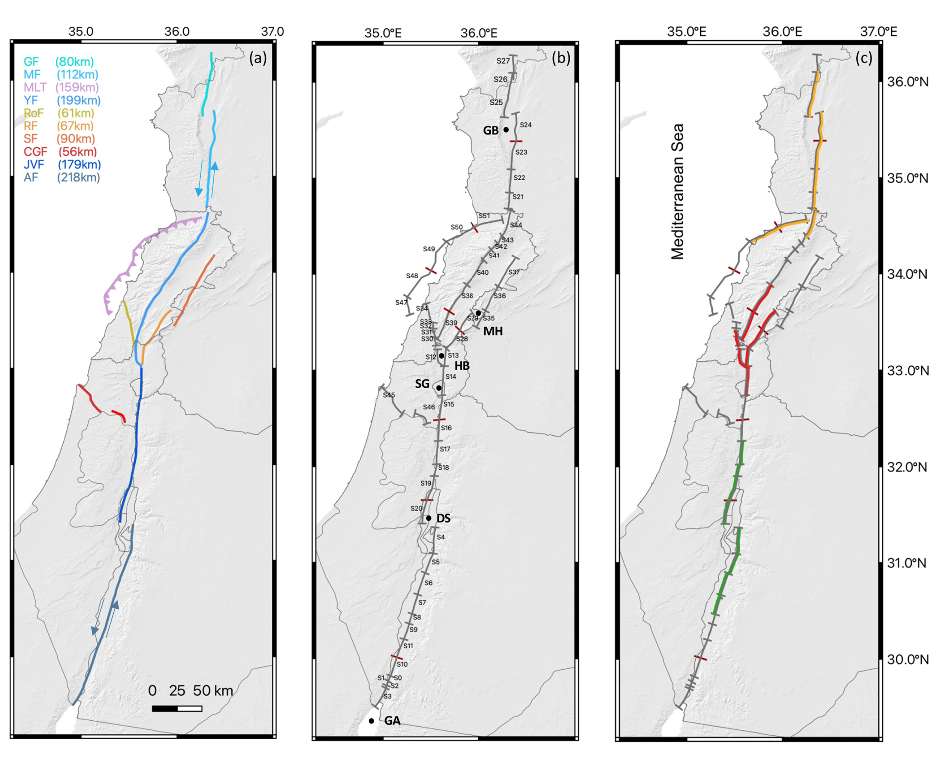
Figure 1 The Levant fault system. (a) Classical fault representation; the fault system is made of 10 main faults, GF: Ghab fault, MF: Missyaf, MLT: Mount Lebanon thrust, YF: Yammouneh, RoF: Roum, RF: Rachaya, SF: Serghaya, CGF: Carmel–Gilboa, JVF: Jordan Valley, AF: Araba (fault map modified from Daëron et al., 2007). (b) Detailed segmentation of the fault system, gray dash: tectonic discontinuities, red dash: arbitrary subdivision of sections required for homogenizing sections' length; GB: Ghab basin, MH: Mount Hermon, HB: Hula Basin, SG: Sea of Galilee, DS: Dead Sea, GA: Gulf of Aqaba (sections provided in the Supplement). (c) Examples of possible complex ruptures that are not accounted for in the classical implementation of faults.

Probabilistic seismic hazard assessment (PSHA) is required to produce seismic hazard maps essential for establishing building codes (e.g., Wang et al., 2016, in Taiwan; Sesetyan et al., 2018, in Türkiye; Beauval et al., 2018, in Ecuador; Meletti et al., 2021, in Italy; or Danciu et al., 2024, within Europe). In most of the source models built for PSHA, the conceptual representation of faults is rigid. Faults are made of a number of tectonically defined sections. Within a predefined fault, ruptures can occur on individual sections or on a combination of sections. However, ruptures that would involve a combination of sections from different predefined faults are not included in the model. The source models therefore usually include only a subset of the potential ruptures that may occur on the fault system.

El Kadri et al. (2023) published a seismic hazard model for Lebanon that integrates the major faults in the area in the classical way described above (Fig. 1a). Earthquake frequencies on these faults are inferred from a moment-balanced recurrence model relying on the geologic or geodetic mean slip rate evaluated for the fault. The source model also includes off-fault seismicity, through a catalog-based smoothed-seismicity model. El Kadri et al. (2023) follow the state-of-the-art standards in PSHA and deliver a distribution of seismic hazard levels for each site within Lebanon, which may be useful for future updates of the Lebanese building code. The present study aims to understand how the source model and eventually the hazard levels may change if an interconnected fault system is considered.

A number of earthquakes in the last 30 years have shown that ruptures can jump over some geometrical discontinuities, such as gaps or steps in the fault system, that were previously considered major obstacles to rupture propagation. These jumps can result in larger magnitudes than anticipated (e.g., 2001 M_w 7.8 Kunlunshan earthquake in China, Klinger et al., 2005; 2010 M_w 7.2 El Mayor–Cucapah earthquake in Mexico, Fletcher et al., 2014; 2016 Kaikōura M_w 7.8 in Aotearoa / New Zealand, Klinger et al., 2018). Therefore, several methods have been developed to take these complex ruptures into account in hazard models. In 2014, the Working Group on California Earthquake Probabilities (WGCEP) developed a new inversion-based methodology called the “Grand inversion” to relax fault segmentation and incorporate multifault ruptures in the Uniform California Rupture Forecast (UCERF; Field et al., 2014; Page et al., 2014). Subsequently, Chartier et al. (2017) implemented the SHERIFS (Seismic Hazard and Earthquake Rate In Fault Systems) algorithm, a method to relax fault segmentation that is simpler than the UCERF framework and that requires fewer input parameters. Additional algorithms were also developed, such as the integer-programming optimization by Geist and ten Brink (2021) or the SUNFiSH approach by Visini et al. (2020). We focus on the SHERIFS algorithm, which has been applied to various crustal fault systems including the Corinth rift in Greece (Chartier et al., 2017), the North Anatolian fault (Chartier et al., 2019), the Eastern Betics in southeastern Spain (Gómez-Novell et al., 2020), the southeastern Tibetan Plateau (Cheng et al., 2021), faults in central Italy (Moratto et al., 2023), and the Pallatanga–Puna fault in Ecuador (Harrichhausen et al., 2024).

Our aim is to build interconnected fault models for the Levant fault system, applying the algorithm SHERIFS, and to estimate the associated hazard levels. We consider the faults described in El Kadri et al. (2023), but rather than including them separately in the hazard calculation, we first go down to the section scale and then evaluate all possible section combinations, for all magnitudes up to the maximum-magnitude earthquake. Our aim is to understand how the iterative process in the SHERIFS algorithm builds the set of ruptures and associated occurrence rates and how it distributes the moment budget over the ruptures with the constraint that earthquake frequencies follow a given distribution at the scale of the system. We show that in order for the maximum-magnitude earthquake to be realistic, the connectivity of the LFS fault system must be fully released. Finally, we derive probabilistic seismic hazard levels by combining our preferred fault model with a set of ground-motion models. To test our source model against observations, we compare the earthquake forecast with the available earthquake catalog at a regional scale and with earthquake sequences observed in paleoseismic trenches at a local scale.

2 The Levant fault system

The Levant fault system (LFS) has been the source of multiple significant earthquakes (Fig. 2), resulting in extensive destruction, surface faulting, and alterations to the landscape. Lefevre et al. (2018) have summarized the known history of major earthquakes along the southern fault section, between the Gulf of Aqaba and the Sea of Galilee, over the last ∼ 1200 years, based on tectonic, paleoseismic, and historical data (see trench sites in Fig. 2). Brax et al. (2019) analyzed the literature on historical events between latitudes 31.5 and 35.5° (approximately from the Dead Sea to the Ghab pull-apart basin). A number of destructive earthquakes occurred, including the 363 earthquake (M ∼ 7.3) that may have ruptured sections on the Araba fault or on both the Araba and the Jordan Valley fault (Ferry et al., 2011; Klinger et al., 2015), the 551 event (M ∼ 7.3) that probably ruptured the offshore Mount Lebanon thrust (Elias et al., 2007), and the 1202 earthquake (M ∼ 7.6) that ruptured the Yammouneh fault (Daëron et al., 2005, 2007) as well a section of the Jordan Valley fault (Jordan Gorge fault; Wechsler et al., 2018). North of Lebanon, strong earthquakes have also occurred along the Missyaf and Ghab faults, in particular the 1170 and 1157 earthquake sequences (Meghraoui et al., 2003; Sbeinati et al., 2010).

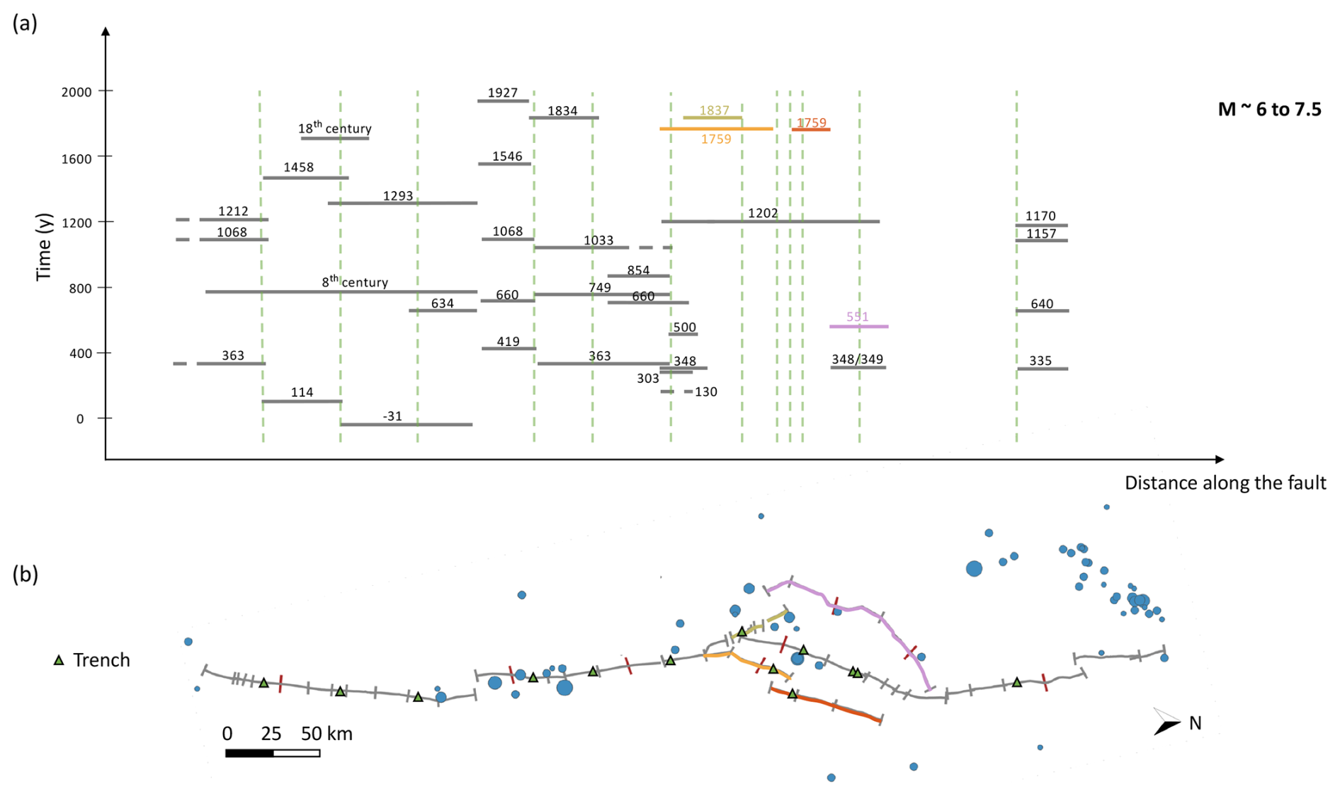
Figure 2 Seismic activity in the region of the Levant fault system. (a) Paleoseismic events (horizontal bars; Lefevre et al., 2018) with extension of the ruptures inferred from observations in the trenches along the fault. (b) Fault system with detailed segmentation, trenches (green triangles), and instrumental events from global datasets (circles, magnitude larger than or equal to 4.1 in the instrumental catalog starting in 1900; see Sect. 6); gray ticks: tectonic discontinuities, red ticks: arbitrary subdivision of sections.

To build the set of ruptures that may occur within the fault system, we need to move away from the regional-scale fault scheme of the LFS (Fig. 1a) and go down to the scale of the tectonic section. Several authors have studied the fault system and analyzed the segmentation. To the south, based on the location of major jogs and bends, Lefevre et al. (2018) proposed to split the Araba and Jordan Valley faults into 9 sections, up to the Hula Basin segment south of Lebanon. Ferry et al. (2011) studied the Jordan Valley section, based on satellite photographs, field investigations, and offset measurements. They mapped in detail the fault trace between the Dead Sea and the Sea of Galilee and identified six 15 to 30 km long right-stepping sections limited by relay zones. Within the Lebanese restraining bend, Daëron (2005) mapped the Yammouneh fault based on satellite images, aerial photographs, and topographic maps. Additionally, the Roum, Rachaya, and Serghaya fault traces were mapped by Nemer and Meghraoui (2006) and Nemer et al. (2008a). through detailed fieldwork and aerial-photograph analysis. Meghraoui (2015) discussed the LFS fault trace and its segmentation, from the Gulf of Aqaba to the Amik Basin in Türkiye, identifying the geometrical complexities (large stepovers, pull-apart basins, restraining bends) that may act as barriers to earthquake ruptures.

We have built on these studies and reanalyzed satellite images along the whole fault system, looking for distinct steps and bends to define the sections. We have carefully analyzed the geological features and incorporated the relevant local paleoseismic information. The LFS mostly exhibits transtensional features, such as the significant pull-apart structures of the Gulf of Aqaba, the Dead Sea (gap width ∼ 14 km), and the Ghab (∼ 11 km). Another major discontinuity is the compressional jog that forms Mount Hermon and separates the Rachaya and Serghaya faults (Fig. 1b). At a smaller scale, the LFS comprises linear strands characterized by left-lateral offsets of drainage systems, right-stepping ruptures exhibiting pressure and shutter ridges, and minor pull-apart basins distributed along its length (such as the Qalaat Al Hosn pull-apart basin at the Syrian–Lebanese border, the Hula Basin, or the Yammouneh basin along the Yammouneh fault). We have also observed push-up zones indicating uplift along the Araba fault. In total, we obtained 43 sections with lengths varying from 5 to 39 km (Fig. 1b, Table 1). Future ruptures may break along one or several sections. For example, a large earthquake could start in the Dead Sea pull-apart basin and propagate bilaterally both to the south on the Araba fault and to the north on the Jordan Valley fault (Fig. 1c, green). A large earthquake could also involve a rupture on the main strand of Yammouneh fault together with ruptures on the Roum and Serghaya fault branches in the same event (Fig. 1c, red). This complexity needs to be included in order to make more realistic fault models for PSHA. The level of connectivity in the system depends on which discontinuities are considered firm barriers for earthquake ruptures.

Table 1 List of the faults, sections, and sub-sections, with corresponding dip, length, and width, as well as mean maximum magnitude (inferred from Leonard 2014) and slip rate estimates (see Fig. 1). The scaling relationship used is from Leonard (2014). Coordinates of sections are provided in the Supplement.

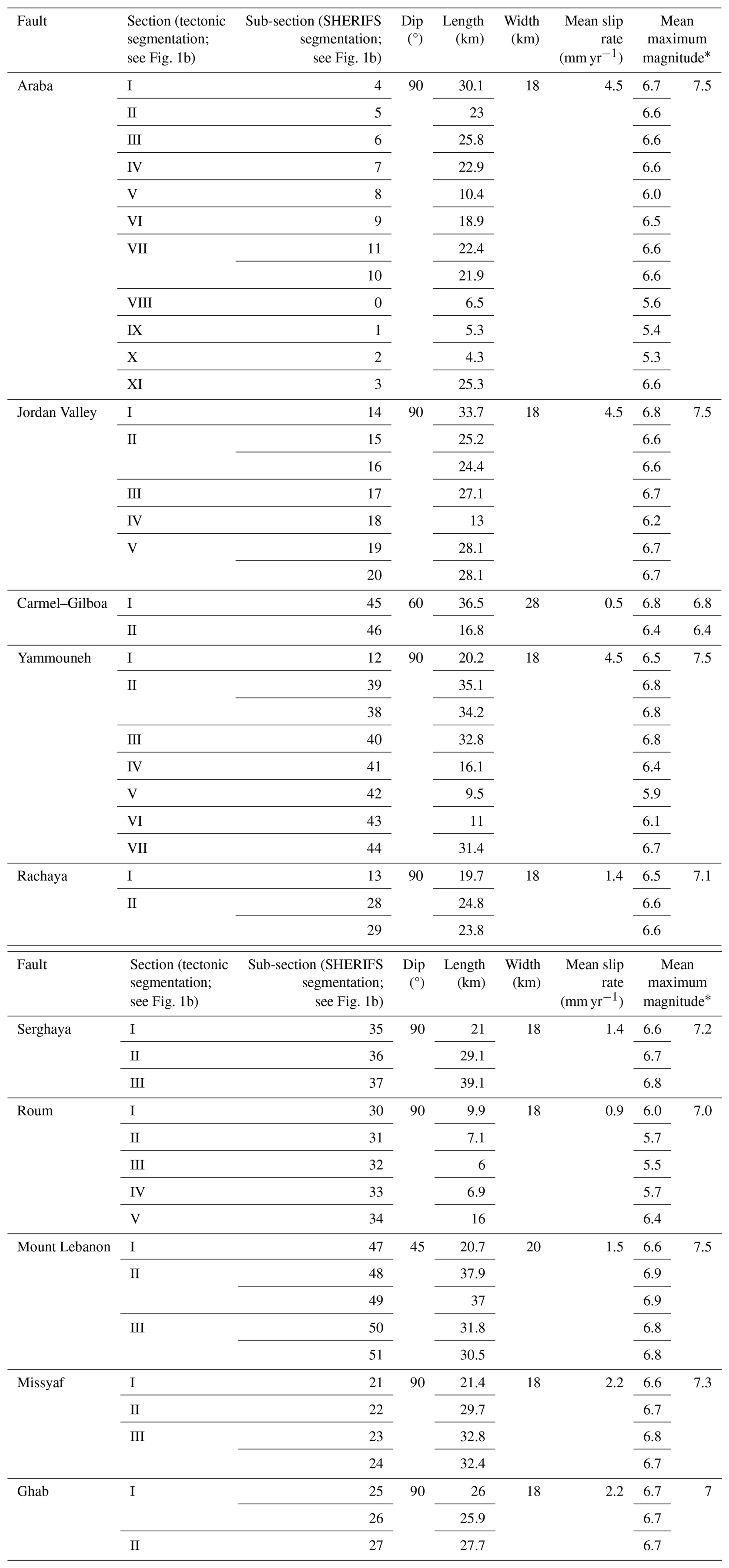
^∗ Strike slip: mean $M_{max}={\log }_{\mathrm{10}}\left(A\right)-\mathrm{2.0087}$ (area A in km²). Reverse: mean $M_{max}={\log }_{\mathrm{10}}\left(A\right)-\mathrm{2.0013}$.

Some faults might be mechanically independent, while others involve faults that interact with each other. The degree of fault interaction is related to the dynamics of the earthquake rupture process (Harris and Day, 1993; Gupta and Scholz, 2000). According to Scholz and Gupta (2000), the probability of an earthquake jumping from one fault to another increases with the degree of stress interactions between the faults. They introduced a criterion to estimate the degree of interaction based on separation and overlap of echelon normal faults and recognized that the case of strike-slip faults is more complex. Wesnousky (2006) studied the mapped surface ruptures of 22 historical strike-slip earthquakes to understand the role of geometrical discontinuities in the propagation of earthquake ruptures and to evaluate the possibility of predicting the endpoints of future earthquake ruptures. Based on this dataset, he showed that ruptures do not propagate across fault steps larger than 3–4 km. However, subsequent earthquakes, such as the 2010 M_w 7.2 El Mayor–Cucapah earthquake in Mexico (Fletcher et al., 2014) or the 2016 M_w 7.8 Kaikoura earthquake (Hamling et al., 2017), have challenged these conclusions and demonstrated that fault systems can undergo complex ruptures, involving numerous faults with various orientations and much larger stepovers. The Levant fault system includes significant discontinuities, with apparent step sizes exceeding 10 km (e.g., Ghab Basin, Mont Hermon, Dead Sea Basin). In the present work we test different levels of connectivity, allowing progressively larger jumps for ruptures. Nonetheless, it is important to keep in mind that within these discontinuities, substantial uncertainty exists regarding the presence of splay faults connecting neighboring faults. Hence, these gaps might be smaller than they currently appear in map view.

3 SHERIFS iterative process

The SHERIFS algorithm (Chartier et al., 2017, 2019) aims at producing an interconnected fault model for PSHA by converting the moment rate stored within the fault system into earthquake rates along the faults. SHERIFS proposes a technique for distributing the moment rate budget over a number of earthquake ruptures within the system, with the constraint that earthquake rates follow a magnitude–frequency distribution (MFD) at the level of the system. This magnitude–frequency distribution can be a Gutenberg–Richter distribution or any other distribution (e.g., characteristic distribution). Ruptures can occur on sections alone or on combination of sections.

The SHERIFS algorithm delivers a set of sections and sections' combinations (ruptures) with associated magnitudes and occurrence rates. In previous applications of SHERIFS, no information has been provided on the obtained distribution of rupture magnitudes in space. Knowing how seismic rates are distributed in space is key to understanding the geographical pattern of hazard levels. In PSHA, at a site, ground-motion exceedance rates are calculated by multiplying rates of ruptures with the probabilities that the ruptures produce an exceedance of the ground-motion levels at the site. Ruptures close to the site will contribute more than ruptures away from the site. In the present study, we aim at understanding the exact distribution in magnitude and space of the ruptures and its link with hazard levels.

The algorithm requires the following as inputs:

• the set of fault sections' traces with extension at depth (dip angles and widths), displayed in Fig. 1b, described in Table 1, and provided in the Supplement;

• the slip rates associated with every section (Table 1);

• the geometrical rules for a section to be able to break with its neighboring sections: the maximum azimuth between two adjacent sections (here we use 75°; Milner et al., 2013, used 60°) and the maximum distance between sections that a rupture may jump (see, e.g., 5 km in Milner et al., 2013; 15 km in Milner et al., 2022);

• an assumption regarding the shape of the magnitude–frequency distribution of the system (here we mainly use the Gutenberg–Richter distribution with a universal b value of 1 (Kagan, 2002), but a characteristic distribution could also be considered);

• the selection of a scaling relationship to associate magnitudes with rupture area (here we use Leonard, 2014, equations for interplate earthquakes);

• an estimate for the maximum earthquake magnitude within the system.

If the length of the sections is too heterogeneous, the algorithm subdivides the longest sections into shorter sections to homogenize sections' length. Within the Levant fault system, nine tectonic sections with length larger than 40 km are arbitrarily subdivided into two sections, resulting in 52 sections in total within the fault system (Fig. 1b). Table 1 summarizes the characteristics of the sections considered. Figure A2 in the Appendix displays the distribution of section lengths. References for the mean slip rates can be found in El Kadri et al. (2023).

The total moment rate budget within the system, to be released in earthquakes, corresponds to the sum over all sections:

$$\begin{array}{}\text{(1)}& \dot{M_{\mathrm{0}}}=\sum _{i=\mathrm{1}}^{i=n}\mathit{\mu }{A}_i{\dot{S}}_i,\end{array}$$

with μ denoting the shear modulus and A_i and ${\dot{S}}_i$ denoting the area and the slip rate of a section, respectively.

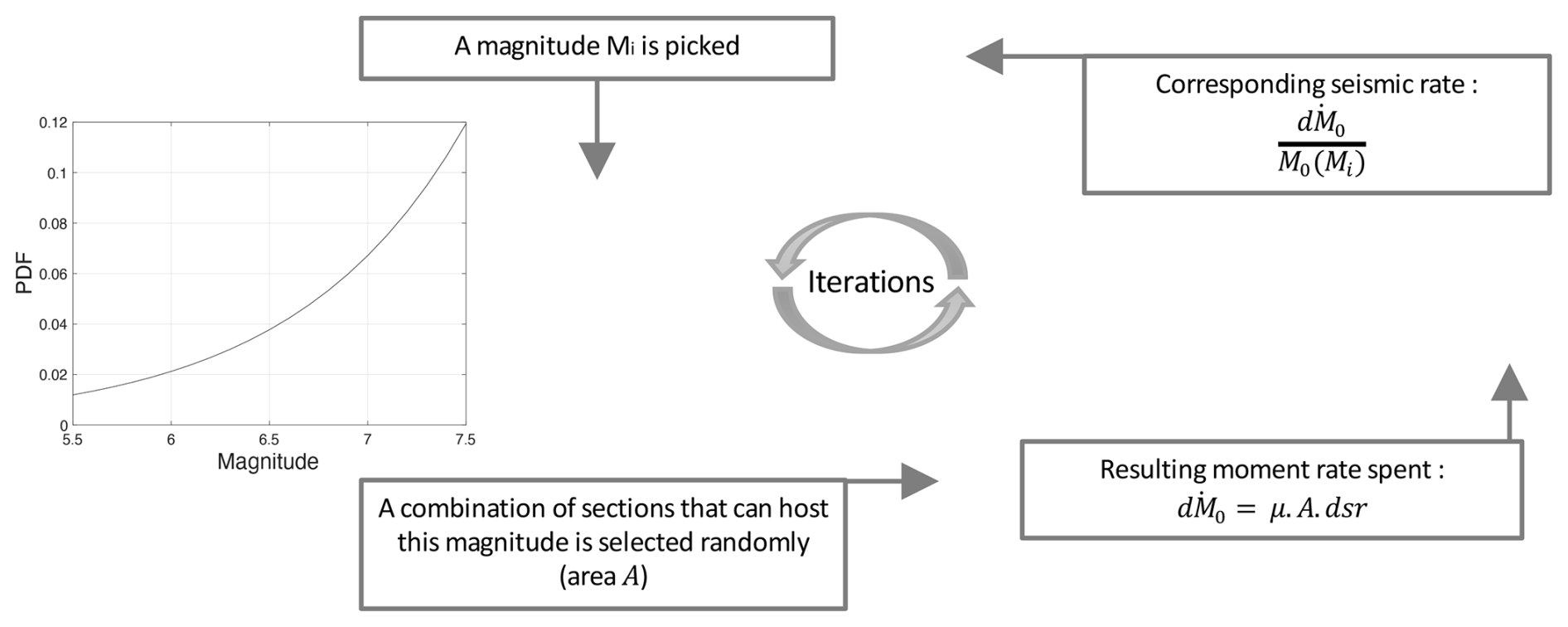
Figure 3 Scheme illustrating the main steps of the SHERIFS iterative process where an amount of slip rate “dsr” must be spent: (1) a magnitude M_i is picked; (2) a combination of one or several sections that can host this magnitude is selected; (3) the associated moment rate is estimated considering the slip rate increment, the area of the rupture A, and the shear modulus μ; (4) the seismic rate is estimated by dividing the moment rate by the moment M₀ corresponding to this magnitude. The iterative process goes on until the sum of all section slip rates is exhausted. PDF to sample the magnitude established considering a Gutenberg–Richter distribution with b value = 1 and M_max = 7.5.

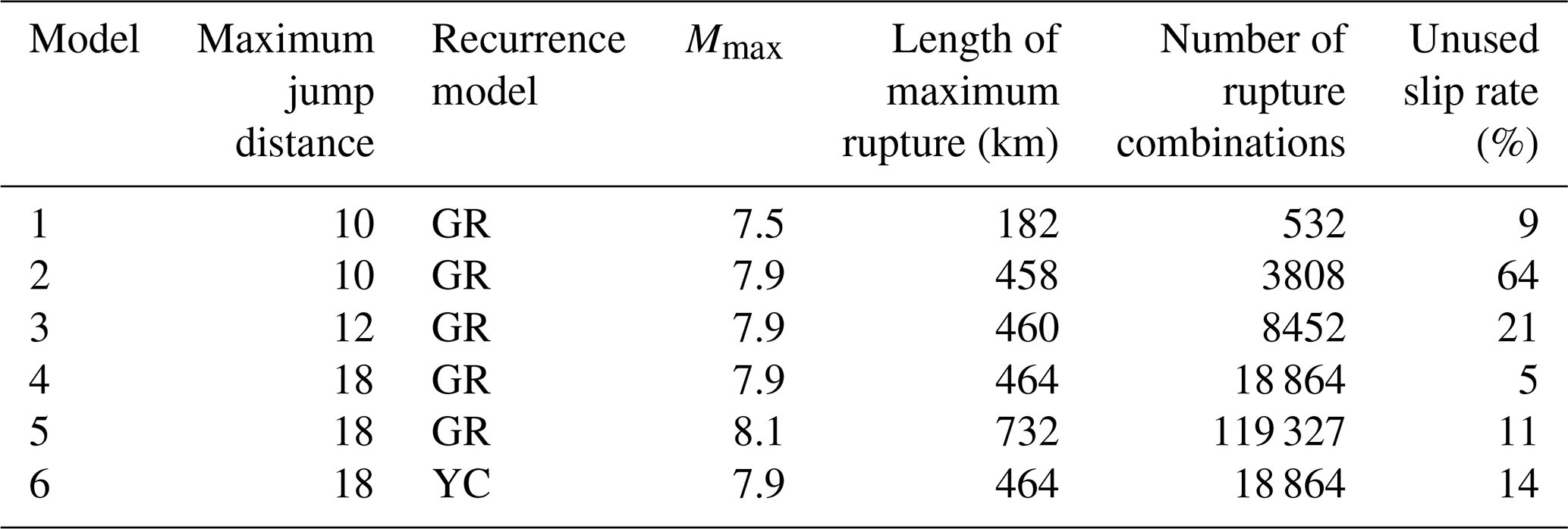
Based on the hypothesis that earthquake rates follow a Gutenberg–Richter distribution, a probability density function (PDF) for the magnitude is built, corresponding to the relative contribution of the magnitude bins in terms of moment rates within the system (Fig. 1 in Chartier et al., 2017). The Gutenberg–Richter model delivers probabilities of occurrence that decrease with increasing magnitude according to an exponential. In SHERIFS, these probabilities are multiplied by the corresponding moment rates, then normalized to obtain the final probability density function used to sample magnitudes in the iterative process. The exponential decrease in rates with increasing magnitudes is compensated for by the huge increase in moment rate with magnitude. In the final PDF, probabilities increase with magnitude (step 1 in Fig. 3, Fig. A1 in Appendix A). Using this PDF to sample magnitudes, large magnitudes are picked much more frequently than low magnitudes.

The moment rate is distributed through an iterative process over magnitudes and associated sections or sections combinations. In a preliminary step, the algorithm establishes all possible ruptures, or section combinations, and associates earthquake magnitudes with these ruptures by applying the area–magnitude scaling relationship. Then, an iterative process starts (Fig. 3) where, at each iteration, the same amount of slip rate is spent (called “dsr”). This process is as follows:

1. A magnitude is randomly picked in the PDF.

2. A rupture is selected randomly from the pool of ruptures with areas matching the magnitude, according to the scaling relationship.

3. The moment rate spent in the iteration is calculated based on the total area of the rupture, the shear modulus, and the slip rate increment (Fig. 3).

4. The seismic rate is eventually obtained by dividing this moment rate by the moment corresponding to the magnitude.

Each time a section participates in a rupture, its slip rate budget decreases accordingly. When a section has no slip rate left, it cannot participate in any new ruptures. The iterative process goes on until the slip rate of all sections in the system is exhausted. Our tests show that the increment in slip rate must be very small to ensure a homogeneous distribution of seismic rates over the system (here we use 0.0001 mm yr⁻¹).

Large magnitudes are picked more frequently than low magnitudes, so the upper range of the system-level magnitude–frequency distribution is first built, then the remaining moment rate budget is spent over lower magnitudes until no budget is left. During the iterative process, at some point the rates of the largest magnitudes stabilize because some sections required to create these large ruptures have their slip rate exhausted. The shape of the magnitude–frequency distribution is anchored to the rates in the upper magnitude range (see Chartier et al., 2017, 2019). As will be shown in the application to the Levant fault system, understanding the role of these “anchor points” is key to fully grasping how the SHERIFS algorithm works and why the moment rate budget can never be spent entirely.

A tapered Pareto distribution (Kagan, 2002) could be used rather than a truncated Gutenberg–Richter distribution, as in the fault models built for the 2019 Italian seismic hazard model (Visini et al., 2021). This distribution includes a bending of the recurrence model from a magnitude called the corner magnitude, rather than a sharp cutoff at a maximum magnitude in the truncated distribution. The tapered distribution usually leads to a stronger decrease in seismic rates in the upper magnitude range with respect to the truncated Gutenberg–Richter distribution. For a fixed moment rate budget, a decrease in rates in the upper magnitude range would lead to an increase in rates in the moderate magnitude range. Using a tapered Pareto rather than a truncated Gutenberg–Richter distribution could lead to slightly different results but would not impact the main findings of the present study. Additionally, we use a b value equal to 1. The choice of the b value may impact the seismic rates obtained; however El Kadri et al. (2023) have shown that using moment-balanced magnitude–frequency distributions with b values within a reasonable range (0.85–1) has little impact on hazard estimates.

In the SHERIFS iterative process, magnitudes are sampled in a PDF at each iteration and associated with a combination of segments (with area matching the magnitude). At the scale of the system, the summed seismic rates follow a Gutenberg–Richter magnitude–frequency distribution (or another MFD shape). However, the set of ruptures and associated rates does not constitute a synthetic catalog (Chartier et al., 2019).

4 First application to the Levant fault system and comparison with the classical implementation

We start with a test that enables comparison with the classical implementation of faults (Fig. 1a). We consider that ruptures cannot jump major discontinuities (Ghab pull-apart basin, Dead Sea pull-apart basin, Mount Hermon jog, gap between the Roum and Mount Lebanon faults); therefore we set the maximum jump to 10 km. All sections can break with their neighbors, except those separated by these four gaps. We consider a maximum magnitude of 7.5 in the system, corresponding to the maximum-magnitude earthquake in the classical implementation of faults, using the mean rupture area predicted by the Leonard (2014) scaling relationship (maximum length ∼ 200 km and width 18 km; Yammouneh, Jordan Valley, and Araba faults; Fig. 1a).

4.1 Iterative process, the system magnitude–frequency distribution (MFD), and the anchor points

Using a slip rate increment of 0.0001 mm yr⁻¹, in total ∼ 1.9 million iterations are required to spend the system slip rate budget. Figure 4 illustrates the process at three different steps. The first column displays, for iteration no. 1500, the moment rate already spent per magnitude interval (Fig. 4a, in blue), earthquake rates distributed within the system (Fig. 4b, in blue), and the fault sections that still have some budget to spend at this stage (in gray, all of them). The second column provides an update at iteration no. 786300, with the moment rate spent and magnitude rates in orange. At that iteration, the rates in the upper magnitude range (i.e., 7.3–7.5) are fixed and the Gutenberg–Richter MFD of the system is anchored to these upper magnitude rates (black straight line). A number of sections have entirely spent their budget (Fig. 4f, in orange), whereas others still have some budget (in gray), but no more large magnitudes (7.3–7.5) can be produced. In subsequent iterations, magnitudes continue to be sampled in the PDF and the remaining slip rate budget is spent until the seismic rates reach the system MFD (Fig. 4h; green crosses align with the black line). Any slip rate increment that leads to higher rates than predicted in a magnitude bin is discarded and considered aseismic slip. The third column displays results at the final iteration: the total moment rate spent (in green), the final magnitude–frequency distribution (in green), and the sections that either have consumed their budget entirely (orange and green) or have part of their slip budget converted into aseismic deformation (in gray).

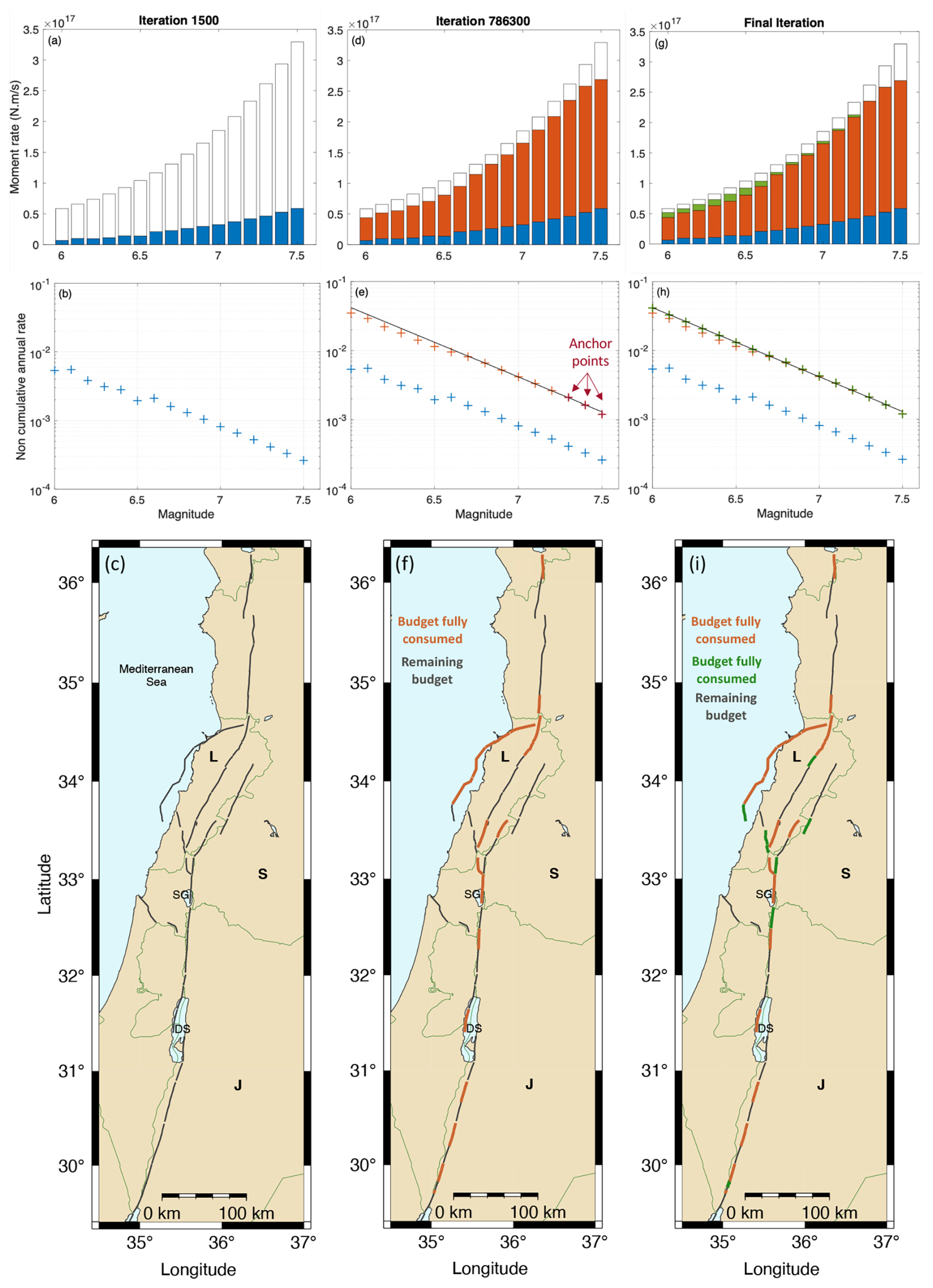
Figure 4 Illustration of the iterative process in SHERIFS, at 2 intermediary steps (first and second column) and final step (third column). The maximum magnitude within the system is 7.5, and the maximum jump is 10 km. First row (a, d, g): in color, moment rate spent per magnitude bin (white: total budget available). Second row (b, e, h): seismic rates distributed over the fault system. Third row (c, f, i): fault sections that still have some budget to spend (gray), sections with slip budget exhausted (orange, then green), in panel (i): end of the process, sections with part of the slip budget converted into aseismic slip (gray). See the text. L: Lebanon, S: Syria, J: Jordan, SG: Sea of Galilee, DS: Dead Sea.

Overall, in this calculation, 9 % of the slip rate budget was not spent on earthquakes. Chartier et al. (2017) call the unused slip rate “non-mainshock slip”. We prefer to simply state that part of the slip rate is not used and is considered aseismic slip. This aseismic slip may correspond to creep or afterslip of major events. Using the term “non-mainshock slip” may imply that this slip could correspond to aftershocks that are not modeled; however aftershocks usually represent a negligible fraction of the total moment rate (see, e.g., Marinière et al., 2021). Chartier et al. (2019) use this unused slip rate as an indicator of whether the model is reasonable or not. Most studies assume that the slip rate deficit along the Levant fault system will be entirely released in earthquakes and that creep is negligible (Gomez et al., 2003; Daëron et al., 2004; Gomez et al., 2007b; Wechsler et al., 2018), so 9 % is an acceptable amount of aseismic deformation.

4.2 The distribution of magnitude rates in space

As in any probabilistic seismic hazard study, we need to know where the seismic rates are distributed in terms of space and magnitude. With SHERIFS, because the moment rate (or slip rate) is distributed across a huge number of ruptures (combination of sections), it is not straightforward to display this information. One solution is to estimate the participation rate of the sections for given magnitude earthquakes. Figure 5 displays the annual rates of occurrence obtained for the participation in magnitude M_w 6, M_w 6.5, and M_w 7.5 ruptures, respectively, for every section of the fault system. Rates are normalized by the section area in order to be comparable throughout the system. We run the SHERIFS algorithm several times, and the distribution of the magnitude rates in space is very similar. Figure 5 shows that whatever the magnitude, the distributions of earthquake ruptures along the system are not homogeneous and rates vary strongly between sections. For magnitudes 6 and 6.5, the highest rates (orange to red) are obtained on the southern half of the Yammouneh fault, southern sections of Jordan Valley fault, and northern sections of the Araba fault. For magnitude 7.5, we observe the opposite: the highest rates are obtained along the northern part of the JVF and along the northern sections of the Yammouneh fault. Owing to the shape of the probability density function, the SHERIFS algorithm is more likely to pick magnitudes in the upper magnitude range than in the lower magnitude range. Sections that participate in large-magnitude ruptures have less slip rate available for moderate-magnitude ruptures. Note that because, for now, ruptures are not allowed to jump gaps larger than 10 km, the sections north of the Ghab pull-apart basin, as well as on the Serghaya fault, cannot participate in a magnitude 7.5 earthquake (in gray in Fig. 5c).

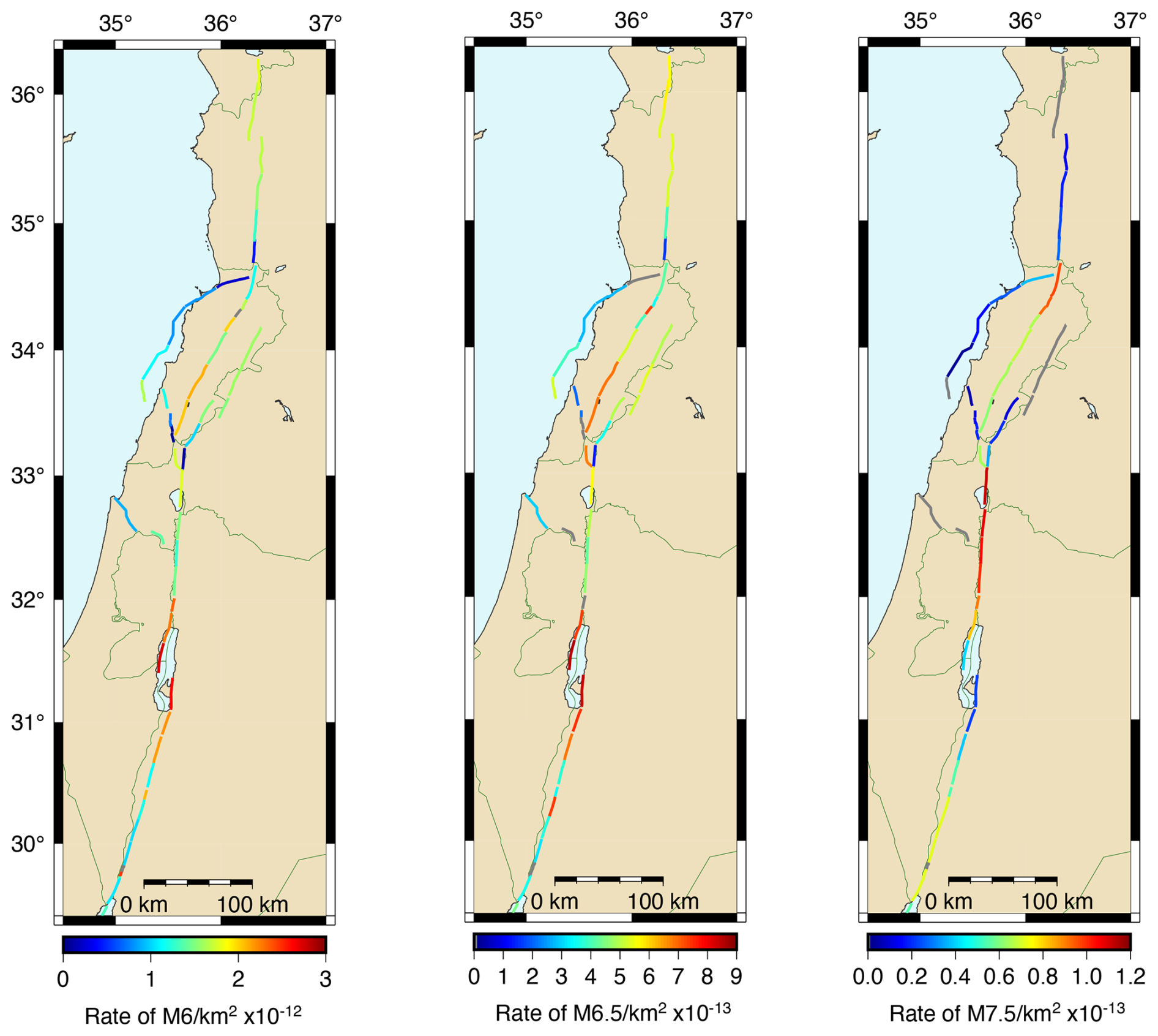
Figure 5 Annual rates of earthquakes for magnitudes M_w 6, 6.5, and 7.5, normalized per square kilometer for each section of the fault system.

4.3 Earthquake rate forecast: interconnected versus classical approach

The moment budget available for earthquakes relies on the slip rates of fault sections and is the same as in the classical implementation of faults. However, the distribution of this moment budget over earthquake ruptures is not similar, as the interconnected fault model includes many more rupture possibilities between sections than the classical implementation. In the interconnected fault model (with maximum jump 10 km), ruptures can combine sections from both the Missyaf and the Yammouneh faults or sections from both the Missyaf and the Mount Lebanon fault. Also, sections that belong to the Roum fault can break with sections on the Yammouneh, Rachaya, and/or Jordan Valley faults. In Fig. 6a, we compare the fault-system MFD obtained with SHERIFS with the fault-system MFD that corresponds to the classical implementation (i.e., the sum of individual Gutenberg–Richter MFDs). We observe that earthquake rates corresponding to the interconnected model are slightly lower in the moderate magnitude range and slightly higher in the upper magnitude range close to M_max. This can be understood by highlighting the sections that can participate in the maximum-magnitude M_max ruptures (Fig. 6b and c, in blue): more sections can participate in a magnitude 7.5 earthquake in the interconnected model than in the classical (rigid) implementation. There is more moment rate available for the upper magnitude range; as the model is moment-balanced, there is slightly less moment rate available for earthquakes in the moderate magnitude range.

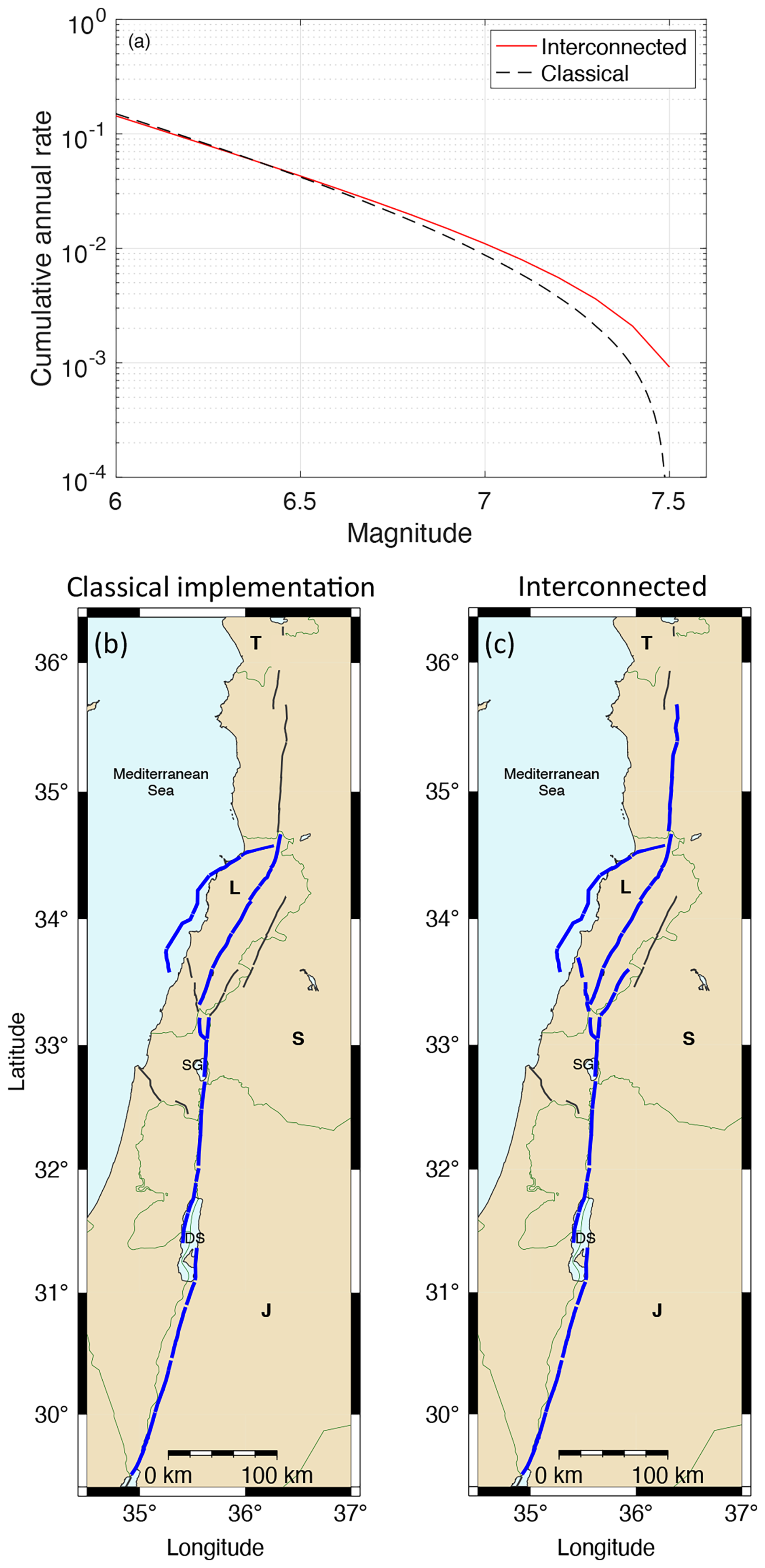
Figure 6 Comparison between the classical implementation of faults and the interconnected model. (a) Magnitude–frequency distributions at the scale of the whole fault system (assumption M_max 7.5); both distributions are moment-balanced using the fault slip rate. (b) Classical and (c) interconnected fault model; in blue are sections that can participate in a maximum-magnitude M_max 7.5 rupture. More sections can participate in the interconnected fault model, so more of the moment rate is available for the upper magnitude range.

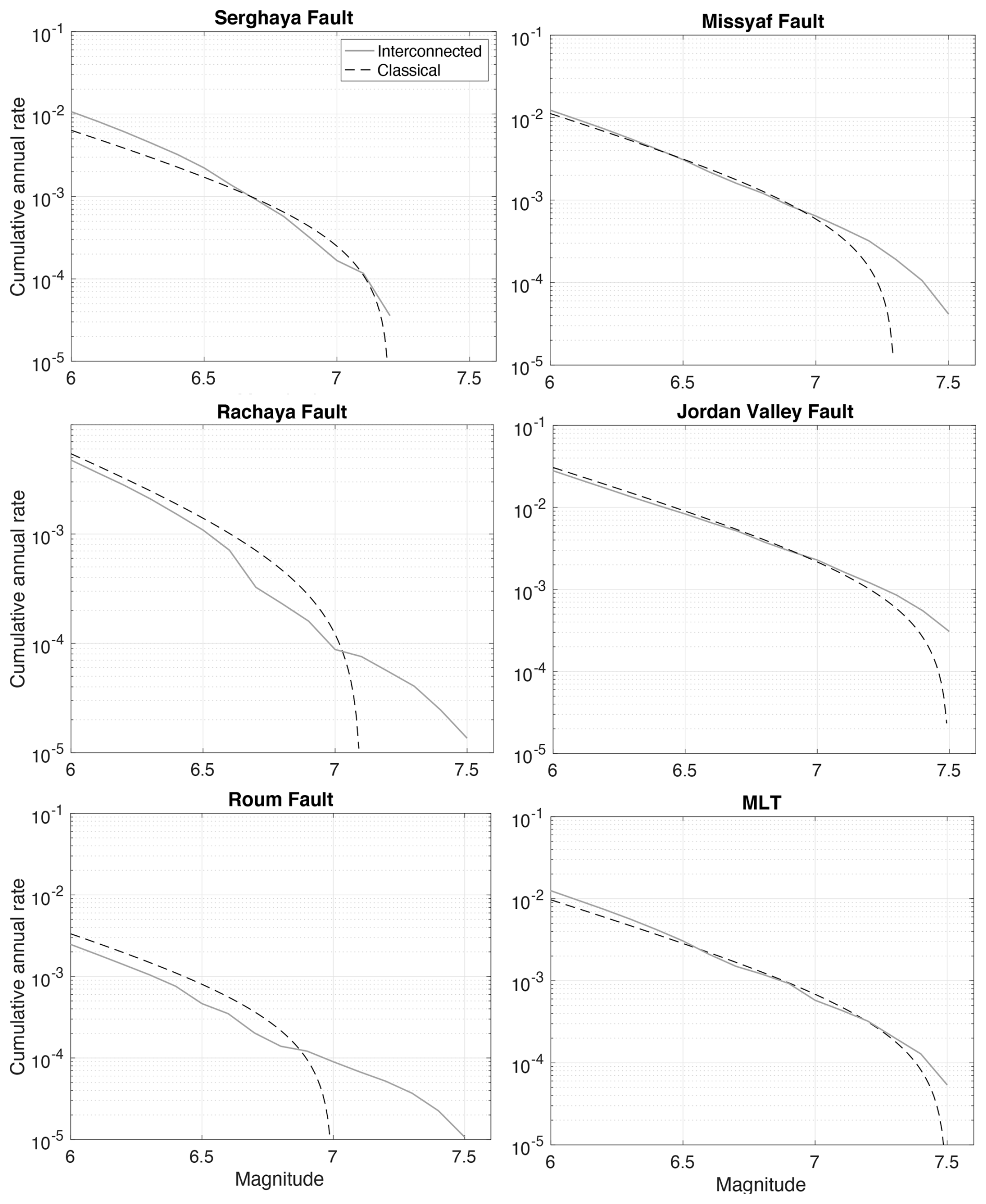
Figure 7 Magnitude–frequency distributions for 6 example faults in the classical implementation (dashed lines), compared to participation rates obtained with SHERIFS (solid lines). Assumption: M_max 7.5. Interconnected model with a maximum jump of 10 km. Participation rates: seismic rates associated with the segments are summed; some ruptures may involve sections that do not belong to the fault.

When performing the comparison at the level of the named faults defined in Fig. 1 (Yammouneh, Rachaya, etc.), the differences obtained between the classical and the interconnected approach are much larger. Figure 7 displays the magnitude–frequency distributions in the classical implementation of faults, superimposed on the participation rates obtained in the interconnected fault model. The sections involved are the same, but in the case of the interconnected fault model, the sections can participate in larger ruptures that include sections from neighboring faults. For example, sections of the Rachaya fault are limited to magnitude 7.1 ruptures in the classical implementation, whereas in the interconnected model, they can participate in ruptures of up to 7.5. As the moment rate budget is the same, the rates in the moderate magnitude range are lower in the interconnected fault model, with respect to the classical fault model.

4.4 Hazard levels at 475 years – interconnected versus classical approach

To compare the classical and interconnected fault models in terms of hazard level, we ran two hazard calculations that combine the same set of ground-motion models with the two different fault models, respectively. Two seismic hazard maps for the peak ground acceleration (PGA) at a 475-year return period were produced (Fig. 8, generic rock site with V_S30 = 760 m s⁻¹). Following El Kadri et al. (2023), we include three ground-motion models equally weighted in a logic tree: Chiou and Youngs (2014), Akkar et al. (2014), and Kotha et al. (2020). The three models predict ground motions for shallow crustal earthquakes. Hazard calculations are performed with the Openquake engine (Pagani et al., 2014). We truncated the Gaussian distribution at 3 standard deviations above the mean.

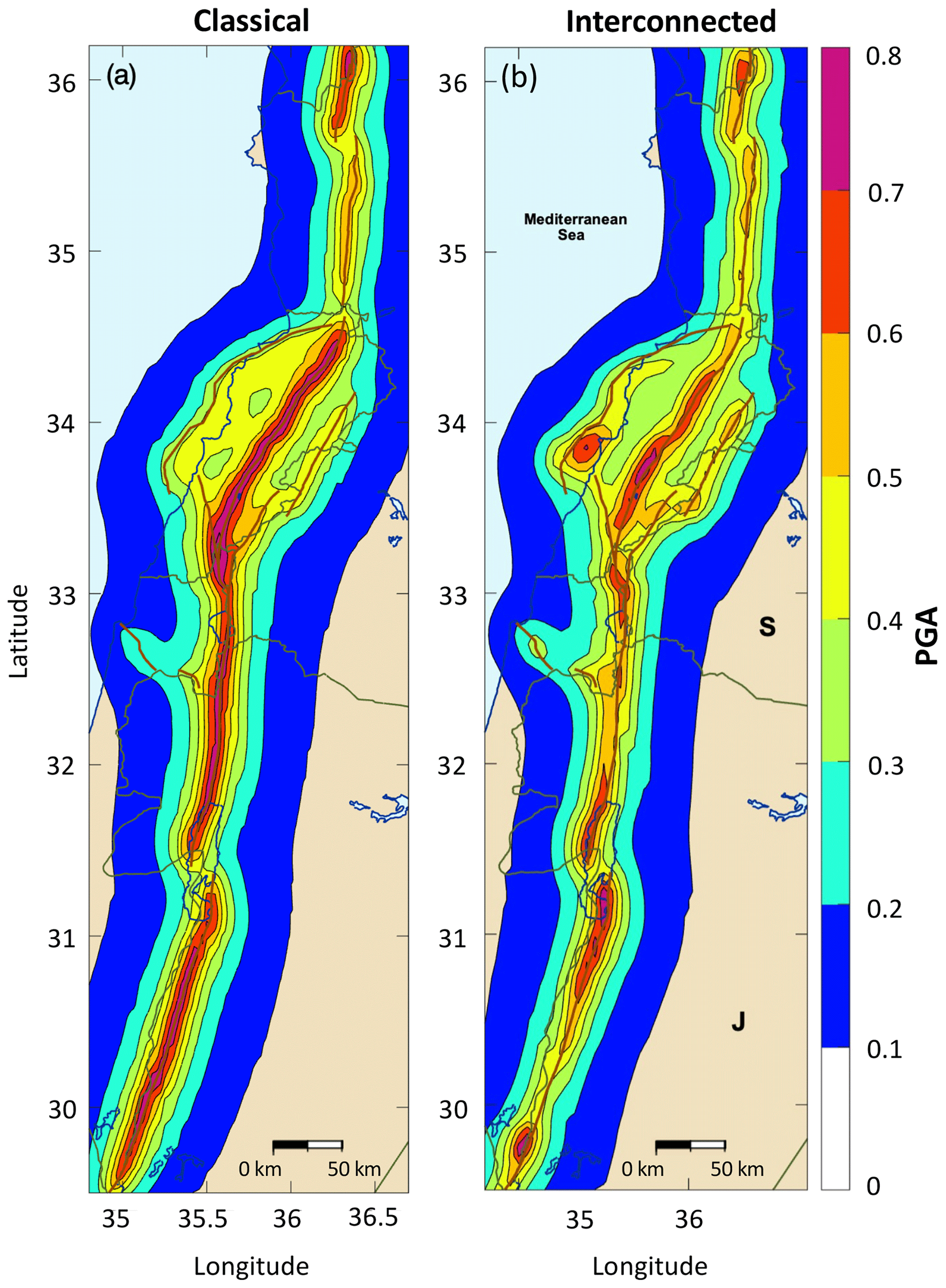
Figure 8 Seismic hazard maps of PGAs at a 475-year return period (a) based on the classical implementation of faults, assuming that the maximum magnitude is M_max 7.5, and (b) based on the interconnected model assuming M_max 7.5 (maximum jump 10 km; ruptures cannot jump major discontinuities). Generic rock site condition (V_S30 = 760 m s⁻¹).

Both seismic hazard maps display peak ground accelerations (PGAs) of 0.7–0.8 g for a mean return period of 475 years, but there are major differences in the hazard patterns obtained. In the classical implementation, the hazard is much higher (up to 0.7–0.8 g) along the more rapid main strand than on the slower branches (up to 0.4–0.5 g), whereas in the interconnected fault model, branches may pose a comparable threat to that of the main strand. Overall, using the interconnected fault model, the hazard levels decrease along the main strand (from ∼ 0.7–0.8 to ∼ 0.5–0.6 g) but increase along the branch faults (from ∼ 0.4 to ∼ 0.5 g), with respect to the classical implementation. In the interconnected model, hazard levels are no longer uniform within a fault: they vary significantly depending on the location of the site along the fault. They are highest along the southern part of the Yammouneh fault, as well as along the southern part of JVF and northern part of Araba fault, corresponding to the sections with the highest rates in the moderate magnitude range (Fig. 5a and b, rates for magnitudes 6 and 6.5). These higher hazard levels can be explained by the observation that moderate magnitudes often control hazard estimates at a 475-year return period, when a Gutenberg–Richter model is used (e.g., El Kadri et al., 2023).

For sites above the dipping Mount Lebanon thrust, the interconnected fault model delivers hazard levels much higher along the southern part than in the north. The northern sections of Mount Lebanon thrust are involved in more large-magnitude ruptures than the southern sections, as they may break with segments from the Missyaf and Yammouneh faults. Southern sections cannot rupture with the Roum fault when the maximum jump is set to 10 km, and as a consequence, annual rates of moderate magnitudes are higher in the south, resulting in higher hazard.

5 Testing different maximum magnitudes for the Levant fault system

Reviewing other major strike-slip fault systems worldwide and the largest earthquakes they have generated (e.g., the 1906 M_w 7.8 earthquake on the San Andreas, Yeats et al., 1997; 2002 M_w 7.9 earthquake along the Denali fault in Alaska, Eberhart-Phillips et al., 2003; or the recent 2023 M_w 7.8 earthquake on the East Anatolian fault, Zhang et al., 2023), we believe magnitudes larger than 7.5 could occur along the Levant fault system. Thus, the source model for PSHA must include the possibility of there being large events, and therefore we test two potential maximum magnitudes: 7.9 and 8.1 (magnitude 7.9 because it is the maximum magnitude observed on a strike-slip fault system, magnitude 8.1 to allow a larger earthquake than observed).

5.1 Test with M_max 7.9 and need for full connectivity

To begin with, we run the algorithm with a maximum magnitude of 7.9, keeping all other parameters as in Sect. 4. In particular, we start with a maximum jump of 10 km. Sections on the Araba, Serghaya, and Ghab faults cannot participate in a magnitude 7.9 rupture (Fig. 9a, sections in blue). Many sections are left with more than 50 % of the slip rate not used (Fig. 9b, sections in orange). Of the total slip rate, 64 % is not spent on earthquakes (Fig. 9b). Such a high percentage of aseismic slip is not realistic in the light of what is known for the LFS. Next, we increase the maximum jump for ruptures from 10 to 12 km and run a new calculation so that ruptures can jump over the Ghab pull-apart basin as well as over Mount Hermon jog (Fig. 9c). All sections can now participate in a magnitude 7.9 earthquake, except for sections on the Araba fault. Only a few end-fault segments are left with more than half of the slip rate unused (Fig. 9d). In this run, 21 % of the total slip rate is not spent on earthquakes.

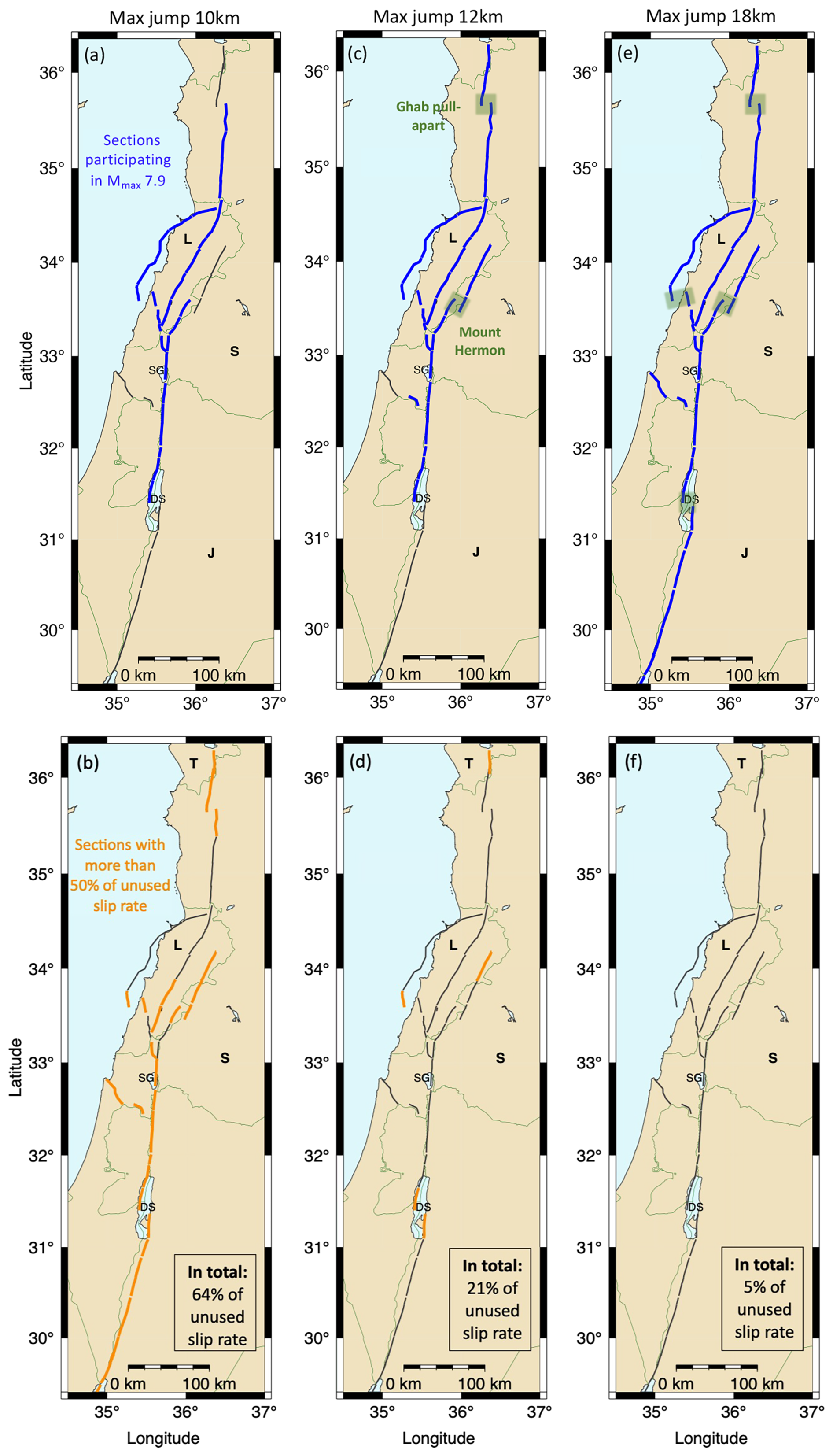
Figure 9 Increasing the connectivity in a fault model with M_max 7.9. First column (a, b): jump up to 10 km allowed. Second column (c, d): jump up to 12 km (ruptures can pass through Ghab pull-apart basin and Mount Hermon jog). Third column (e, f): jump up to 18 km (entirely connected; ruptures can pass all major discontinuities). First row (a, c, e), blue: sections that can participate in an M_max 7.9 rupture, green: discontinuities that ruptures can pass. Second row (b, d, f), orange: sections left with more than 50 % unused slip rate at the end of the run; the percentage of the slip rate not used at the scale of the fault system is indicated.

Lastly, we increase the maximum jump to 18 km so that the fault system is now entirely connected and ruptures can jump over all major discontinuities, including the gap between the Roum and Mount Lebanon faults (Fig. 9e). All sections can participate in a magnitude 7.9 rupture. In this case, the interconnected fault model uses 95 % of the slip rate budget, with 5 % of the budget considered aseismic slip. This low fraction of aseismic slip is compatible with the studies showing that this fault system is nearly entirely coupled (e.g., Wechsler et al., 2018; Al Tarazi et al., 2011).

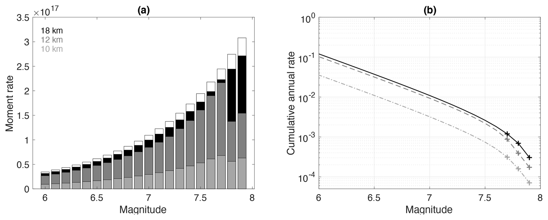
Figure 10 Increasing the connectivity in a fault model with M_max 7.9, (a) distribution of the moment rate spent per magnitude bin and (b) magnitude–frequency distribution, at the scale of the fault system. Light gray: ruptures cannot jump more than 10 km (Fig. 9a), dark gray: maximum jump for ruptures of 12 km (Fig. 9c), black: maximum jump 18 km and system is entirely connected (Fig. 9e).

Figure 10 displays the distribution of the moment rate spent in earthquakes as well as the fault-system MFDs obtained for the three different runs. Increasing the connectivity from a 10 km maximum jump (light gray histogram) to a 12km maximum jump (dark gray histogram) or a 18 km maximum jump with full connectivity (black histogram), the moment rate spent in earthquakes increases. When full connectivity is applied, the moment rate spent (black histogram) is close to the total moment rate stored in the system (white histogram). When ruptures cannot jump over major discontinuities (Fig. 9a), only a fraction of the sections can participate in the maximum-magnitude earthquakes. Thus, rates for earthquakes in the upper magnitude range are low (Fig. 10b, light gray crosses). These rates constitute the anchor points of the system MFD and thus limit the rates over the whole system (light gray dash-dotted curve). Increasing connectivity, more sections can participate in the maximum-magnitude earthquakes, the system MFD is anchored on higher rates, and more moment rate can be spent on earthquakes within the whole magnitude range (dashed dark gray curve for 12km jump, solid dark curve for full connectivity, Fig. 10b).

5.2 Selection of the model with lowest aseismic deformation

In our last test, we kept a fault system entirely connected and increased the maximum magnitude to 8.1. Figure 11 summarizes the tests achieved and displays the system MFD resulting from

• a run with M_max 7.5 and major discontinuities acting as barriers (Sect. 4),

• a run with M_max 7.9 and a fully connected system,

• a run with M_max 8.1 and a fully connected system.

The moment rate available for earthquakes within the system is constant (proportional to the slip rates and section surfaces); therefore when increasing the maximum magnitude of the Gutenberg–Richter model, the rates of moderate-magnitude earthquakes decrease. Earthquakes with magnitude close to 8.0 are believed to have possibly occurred in the past along the Levant fault system (e.g., Lu et al., 2020). Moreover, based on interferometric time-series analysis of satellite radar images, Li et al. (2024) have shown that no significant aseismic slip can be measured anywhere along the entire system. Therefore a 5 % percentage of aseismic deformation is more realistic than 9 % or 11 % for the Levant fault system. The fully interconnected fault model with maximum-magnitude earthquake 7.9 is our preferred model. Next, we calculate the hazard levels obtained when combining this fault model with a set of ground-motion models.

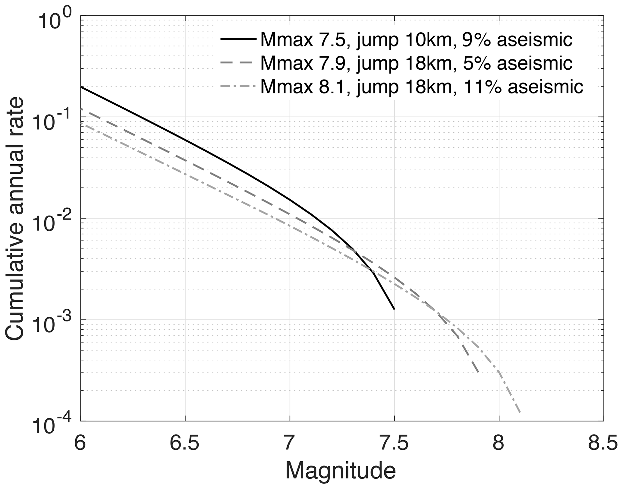
Figure 11 Magnitude–frequency distribution obtained at the scale of the fault system, for three runs of SHERIFS. Solid curve: assumption M_max 7.5 and the major discontinuities act as barriers (Sect. 4). Dashed curve: assumption M_max 7.9 and the system is entirely connected. Dash-dotted curve: assumption M_max 8.1 and the system is entirely connected. All models are moment-balanced, but the percentage of unused slip rate varies with the model (9 %, 5 %, and 11 %, respectively). Our preferred model is the fully interconnected model with M_max 7.9 (see the text).

This is an exploratory study aimed at understanding how the algorithm SHERIFS works. In a probabilistic seismic hazard study aimed at delivering seismic hazard levels for a country, we would populate the source model logic tree with these alternative models to cover the epistemic uncertainty (attributing larger weight to the model associated with the lowest aseismic deformation).

5.3 Hazard levels associated with our preferred fault model (M_max 7.9 and full connectivity)

Figure 12 displays the seismic hazard map obtained for the PGA and 0.2 s spectral acceleration at a 475-year return period by combining the M_max 7.9 interconnected model with the ground-motion logic tree. As expected, the PGA levels for the 475-year return period are lower than obtained from the model with M_max 7.5 (Fig. 8b) due to the decrease in seismic rates in the moderate magnitude range (Fig. 11). At all sites within ∼ 20 km of the faults, PGA values are above 0.3 g, except on the northern part of Mount Lebanon fault inland. PGA values are larger than 0.4 g at most sites along the Ghab fault, Yammouneh fault, the southern part of Mount Lebanon fault, the central part of Jordan Valley fault, and the Araba fault. Peak values above 0.5 g are found mainly at sites along the southern sections of the Mount Lebanon fault, as well as to the north and to the south of the Araba fault. These peak values are likely due to higher rates of moderate magnitudes on these sections. Figure 12b displays spectral accelerations at 0.2 s for the same return period of 475 years.

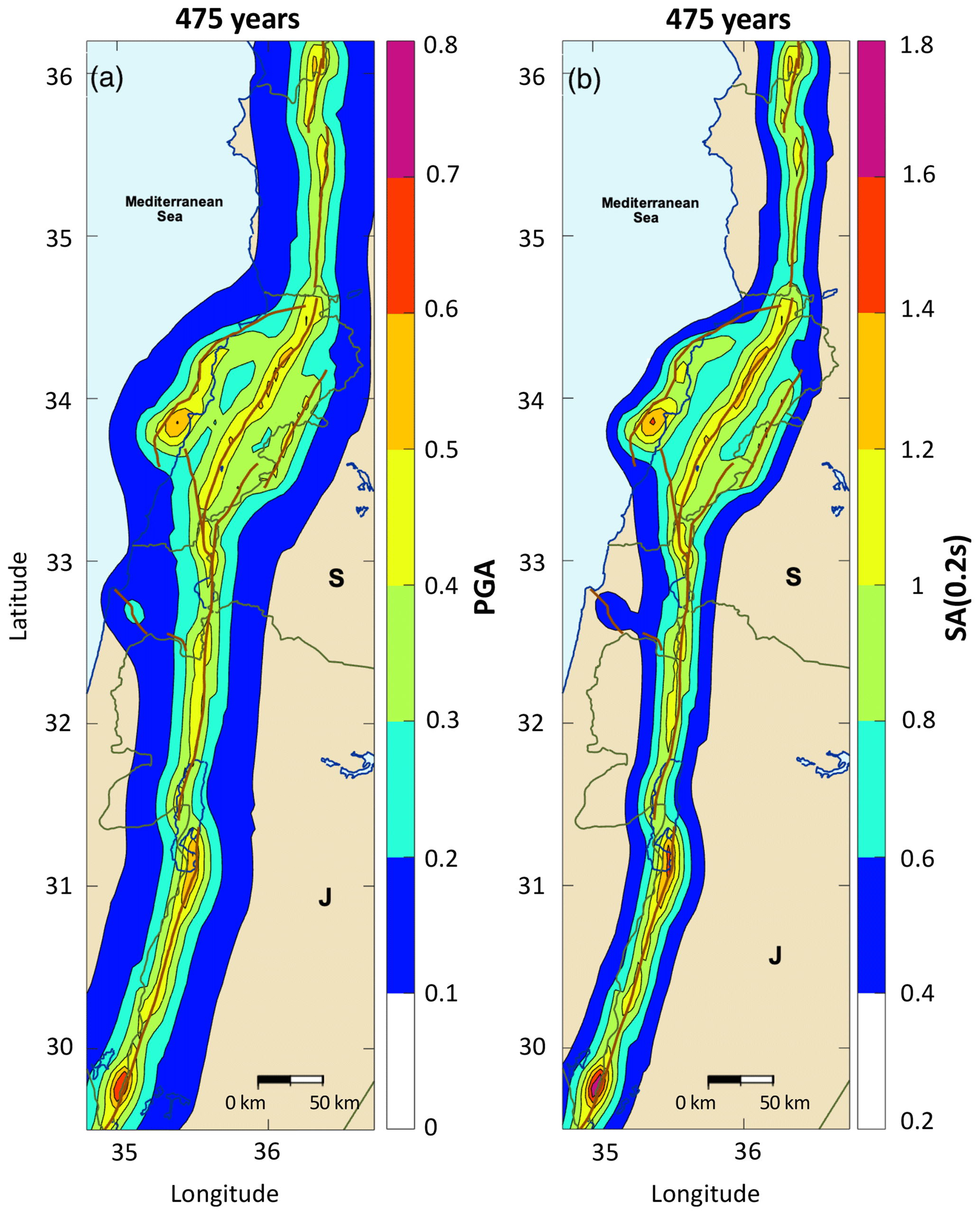
Figure 12 Seismic hazard map for a return period of 475 years based on a fully interconnected model assuming M_max 7.9. (a) At the PGA and (b) at 0.2 s spectral acceleration. Generic rock site condition (V_S30=760 m s⁻¹).

6 Comparison of the modeled rates with the available observations

The earthquake forecast delivers a magnitude–frequency distribution at the scale of the fault system that follows a given shape, here a Gutenberg–Richter model with a b value of 1. This magnitude–frequency distribution is moment-balanced with the long-term slip rates. Long-term slip rates on strike-slip faults are mainly established from geomorphologic data (see El Kadri et al., 2023). Slip rates can be inferred from trenching only if a long time series of earthquakes with a measurement of slip per event is available, which is the case only for the Jordan Gorge section from 3D trenching (Wechsler et al., 2018). Both the earthquake catalog of the region and the available paleoseismic data were not directly used to derive the model; these observations can be compared with the earthquake forecast.

6.1 Observed earthquake rates for the region

Our model forecasts earthquakes on the fault system, and at this stage no background seismicity is added. We build an earthquake catalog for the region keeping in mind that only the largest magnitudes may be associated with the main faults.

Brax et al. (2019) published a catalog of historical earthquakes for the Lebanese region between latitudes 31.5 and 35.5°. For every earthquake, the authors evaluated the information available in historical accounts, as well as the macroseismic intensity datasets produced and their interpretations in terms of epicentral location and magnitude estimate. Earthquakes whose existence is attested but for which it was not possible to find a solution relying on clearly identified historical sources and intensity data have not been included (see Supplement 2 in Brax et al., 2019). For the period before 1900, we used the Brax et al. (2019) catalog, supplemented south of latitude 31.5° and north of latitude 35.5° by earthquake solutions from the EMME earthquake catalog (Zare et al., 2014), resulting in 23 earthquakes in total (Figs. 2 and 13).

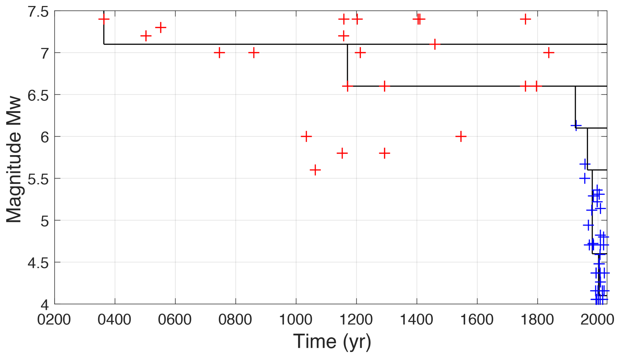
Figure 13 Earthquake catalog used (same as in Fig. 2), magnitude versus time, historical (red) and instrumental (blue) events. Periods of completeness per magnitude interval are indicated (straight lines).

We used global instrumental catalogs over the period 1900 to 2020, within the spatial window of 34.5 to 37° in longitude and 29 to 37° in latitude. We consider the ISC-GEM (International Seismological Center – Global Earthquake Model, Version 10; Storchak et al., 2015), GCMT (Global Centroid Moment Tensors; Ekström et al., 2012), and ISC (International Seismological Centre; Storchak et al., 2020) catalogs. From the ISC catalog we include only earthquakes with an ISC location and a magnitude M_S or m_b (that we convert into M_w applying equations from Lolli et al., 2014). We obtain 35 instrumental events with magnitude M_w ranging from 4.1 to 6.1 (Fig. 13).

Figure 13 displays the earthquake catalog obtained: a number of destructive earthquakes with magnitudes larger than or equal to ∼ 6.5 occurred in the last 2000 years in the region. The last one within this spatial window struck southern Lebanon in 1837. Magnitudes of historical earthquakes bear large uncertainties (see, e.g., Brax et al., 2019); nonetheless such high magnitude levels are confirmed by the analysis of numerous paleoseismic trenches available along the LFS. The distribution of magnitudes in the interval 5.5–6.5 is particularly irregular over time. In the instrumental period starting in 1900, the largest earthquake in the spatial window is the 1927 M_w 6.1 Jericho earthquake (magnitude from the ISC-GEM catalog). The instrumental catalog also bears significant uncertainties as only global data have been included. Brax et al. (2019) did include earthquake solutions from local networks in the region. Different magnitude types are provided, and to merge the datasets, several conversions between magnitudes are required (see Supplement 3 in Brax et al., 2019). The dispersion observed in the magnitude comparisons is very large in most cases. In this study, we prefer to use only global catalogs and ensure a certain level of homogeneity in the magnitude estimate, at the cost of a higher magnitude of completeness.

Earthquake rates are estimated considering a magnitude interval of 0.5. Based on plots of the cumulative number of events versus time, we evaluate that magnitudes larger than or equal to 7.1 are complete since 363 CE, magnitudes larger than or equal to 6.6 are complete since 1170, magnitudes larger than or equal to 4.6 are complete since 1981, and magnitudes larger than or equal to 4.1 are complete since 2003 (Fig. 13). For the magnitude interval 5.6–6.6, there are too few earthquakes to estimate the period of completeness. We estimate periods from the ISC-GEM catalog at the global scale: magnitudes larger than or equal to 5.6 are considered complete since 1965, and magnitudes larger than or equal to 6.1 are considered complete since 1925. Additionally, to get a rough estimation of the impact of magnitude uncertainties in rates, we generated 100 synthetic catalogs from the original one, sampling the magnitude of each earthquake from a Gaussian distribution centered on the original magnitude with a standard deviation of 0.3 for historical events and 0.1 for instrumental events.

Cumulative annual rates are displayed in Fig. 14, superimposed on the modeled magnitude–frequency distribution for the fault system (our preferred model with M_max 7.9 in orange). The rate estimates from an analysis of paleoseismic trenches are also superimposed (Lefevre et al., 2018). We assume that all events with magnitude larger than or equal to 7.1 and most events with magnitude larger than or equal to 6.1 occurred on a known fault. The model is roughly consistent with observations for magnitudes larger than or equal to 6.6, but it forecasts more events than observed for magnitudes larger than or equal to 6.1. Up to now we have tested only the Gutenberg–Richter exponential distribution for the system. To know if a characteristic Youngs and Coppersmith (1985) distribution would be more compatible with observed rates, we again run the algorithm with an M_max of 7.9, full connectivity, and a characteristic earthquake model. The model obtained is roughly consistent for magnitudes larger than or equal to 7.1 but strongly underpredicts rates for magnitudes larger than or equal to 6.6 and 6.1. Of the total slip rate, 14 % is not used and is considered aseismic, which is not realistic.

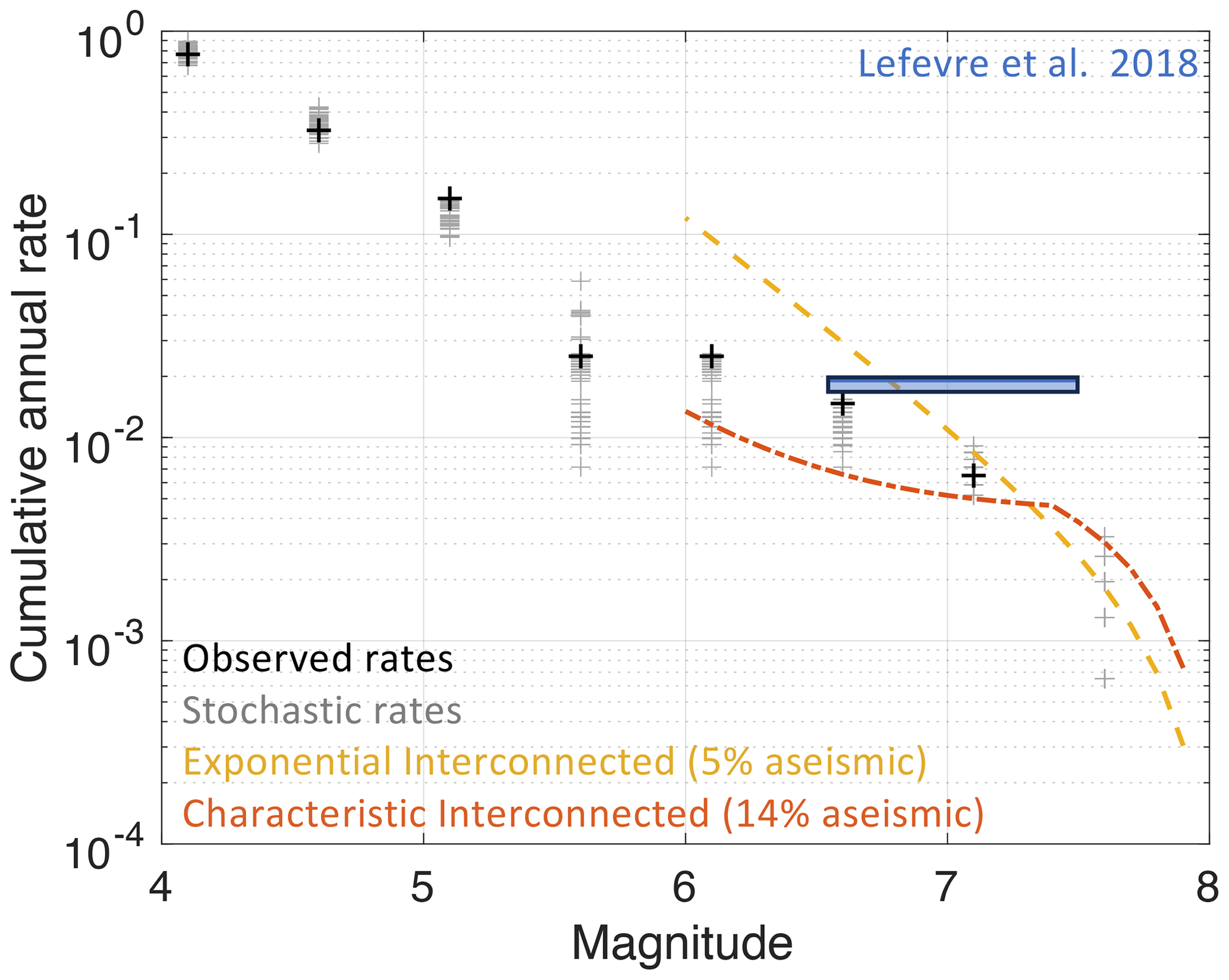
Figure 14 Magnitude–frequency distributions compared to observed rates. Black crosses: observed annual rates estimated from the regional earthquake catalog, gray crosses: annual rates from synthetic earthquake catalogs to account for uncertainties in magnitudes. Orange dashed curve: fault-system MFDs, assumption Gutenberg–Richter, model with M_max 7.9. Red dashed curve: fault-system MFDs, assumption characteristic model Youngs and Coppersmith (1985) with M_max 7.9. Blue bar: mean recurrence times inferred from paleoseismic trenches (Lefevre et al., 2018).

6.2 Earthquake rates from paleoseismic trenches

Paleoseismic studies provide information on earthquakes that occurred before historical times and thus extend the observation time window available. Several trenches have been excavated along the Levant fault system. They deliver key data on the size and on the timing of the earthquakes that ruptured the fault at the trench site. From the fault model built with SHERIFS, we can extract the set of ruptures passing through the trench site, with associated rates, and we compare this forecast with the paleoseismic data.

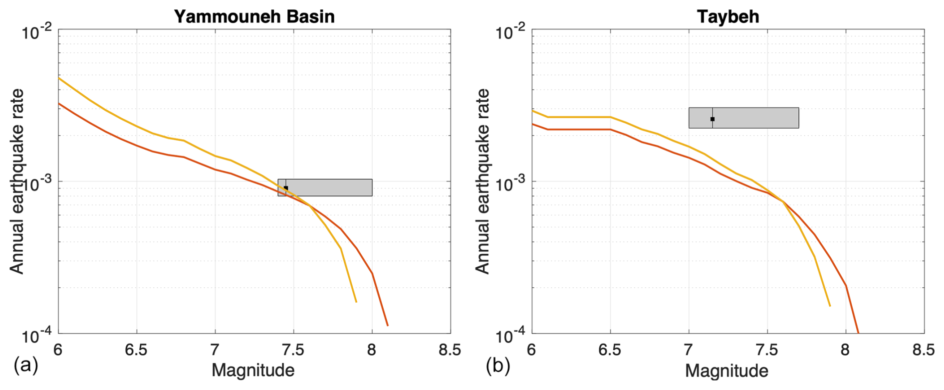
Figure 15 Comparison of the earthquake forecast with rates of earthquakes based on paleoseismic data at two trench sites along the main strand of the LFS. Solid orange line: rates of ruptures passing through the site, as forecasted by the fault model built (also called “participation rates”), a fully interconnected model with M_max 7.9 for the Gutenberg–Richter system MFD. Red line: fully interconnected model with M_max 8.1 for the Gutenberg–Richter system MFD. Rectangle: distribution for the mean inter-event time between large earthquakes, inferred from the paleoseismic data, taking into account the uncertainty in the ages. (a) Trench in Yammouneh Basin located along section S40; (b) Taybeh trench site on section S8 on the Wadi Araba fault (see Fig. 1b and Table 1).

Daëron et al. (2007) analyzed a trench across the Yammouneh basin in detail. They identified 10 to 13 paleo-events extending back more than ∼ 12 kyr, and they were able to provide reliable age bounds for half of these events. In the historical period, the most recent event is the 1202 destructive earthquake (magnitude estimate 7–7.8, according to Ambraseys and Jackson, 1998). They also identified an earthquake that occurred between 30 BCE and 469 CE. We consider these two earthquakes in the historical period, as well as 6 prehistoric earthquakes that occurred in a period extending over ∼ 5600 years starting ∼ 12 kyr ago (record considered complete over the period, events S7 to S12; see Daëron et al., 2007). Estimates for six inter-event times are thus available. To take into account the uncertainty in the age of these events, we generate synthetic earthquake sequences by sampling the age of each event within a uniform PDF defined by the minimum and maximum age bounds (following Ellsworth et al., 1999; see Nemer, 2023). For each synthetic sequence, a mean inter-event time is calculated. We use 1000 synthetic sequences to produce a distribution for the mean inter-event time. In Fig. 15, this distribution is superimposed on the rates of ruptures passing through the site, as forecasted by our preferred fault model (M_max 7.9, entirely connected). Daëron et al. (2007) evaluated a characteristic coseismic slip of about 5.5 m, which according to Leonard (2014) corresponds to an interval of magnitude 7.4 to 8 (extension of the gray box on the graphic). Accounting for the uncertainty in the paleoseismic rates, the observations in the trench are compatible with the forecasts resulting from both the 7.9 and the 8.1 maximum-magnitude assumptions.

Lefevre et al. (2018) conducted a paleoseismological excavation at the Taybeh site, situated on the Wadi Araba fault, that reveals evidence for 12 surface-rupturing earthquakes spanning the last 8000 years. To build the distribution of mean inter-event times, we use the most complete and reliable part of this earthquake sequence, i.e., the period starting with the 31 BCE earthquake that includes 5 earthquakes. To evaluate a magnitude range for these earthquakes, we use the rupture lengths obtained in Lefevre et al. (2018) by correlating the information at different trench sites (gray box in Fig. 15). Our fault model forecasts fewer earthquakes than “observed” at the Taybeh site.

We have compared the forecast to the data observed at two trench sites. A number of other trenches have been excavated along the Levant fault system (e.g., Nemer et al. 2008b; Wechsler et al., 2014; Sbeinati et al., 2010). For a complete evaluation, the forecast should be compared to observations at all paleoseismic sites available. However, such a comparison is beyond the scope of the present article; it should be considered in future developments of hazard models for the Levant fault system.

Table 2 Different parameterizations tested in the application of the SHERIFS algorithm on the Levant fault system. Seismogenic depth considered: 18 km for the strike-slip segments (width of ruptures), 14 km for segments on the Mount Lebanon thrust. GR: Gutenberg–Richter, YC: Youngs and Coppersmith (1985). Slip rate increment (dsr) used: 0.0001 mm yr⁻¹.

7 Conclusions

The classical way of implementing faults in PSHA, considering separate faults that cannot interact with each other, is not realistic. In the future, fault models in PSHA must account for complex ruptures, but there is no standard method yet. A few algorithms have been proposed to distribute the moment rate over the physically possible ruptures, and SHERIFS (Chartier et al., 2017, 2019) is one of them. This algorithm is being increasingly used (e.g., Gómez-Novell et al., 2020; Cheng et al., 2021; Moratto et al., 2023; Harrichhausen et al., 2024); however none of the works published up to now have analyzed the distribution of seismic rates in magnitude and in space that controls hazard levels, nor have they analyzed the results in light of the classical implementation of faults which represents the bulk of PSHA studies at present (both in research and in the industry). The aim of this article is to address these issues.

We test different maximum magnitudes and different shapes for the frequency–magnitude distribution at the fault-system level, as summarized in Table 2. We show how the algorithm distributes the seismic rates over the fault system, applying rules for defining which segments can break together. We demonstrate how some key decisions impact the seismic rates, such as the decision regarding the maximum magnitude the system can produce or the maximum distance ruptures can jump between segments. The conversion of the slip rates into earthquakes is not straightforward; we display seismic rates maps that help us understand the process. Our tests show that the seismic rates associated with a given segment depend strongly on the precise location of the segment within the fault system, as well as on the segment combinations it can be involved in. Hence, hazard levels are directly related to the implementation of the fault system, the system's segmentation, and the decision regarding which segments may break together.

We perform a comparison of a classical fault model implementation with an interconnected fault model, in terms of the distribution in space of seismic rates for different magnitude levels and in terms of seismic hazard levels. Both models are moment-balanced, taking into account fault slip rates. We find that hazard levels may decrease or increase with respect to the classical implementation, depending on the location of the segment within the system (main strand, secondary strand, segment combinations). For the Levant fault system, hazard values at a 475-year return period on average decrease along the main strand (characterized by a slip rate of ∼ 4–5 mm yr⁻¹) and increase along the branches (characterized by a slip rate of the order of ∼ 1–2 mm yr⁻¹). One main difference between the models is that the distribution in space of seismic rates is not homogeneous in the interconnected model, even for moderate-magnitude earthquakes (M 6). These moderate-magnitude earthquakes control hazard levels at a 475-year return period. We find highest hazard levels along segments with the highest seismic rates in the moderate magnitude range.

Among the fault models tested, our preferred model is based on a maximum magnitude of 7.9 and a fully interconnected fault system. Of the total slip rate, 5 % is not spent on earthquakes, which is a reasonable amount for aseismic creep along the Levant fault system. Combining this interconnected fault model with a set of ground-motion models valid for the region, hazard levels have been estimated. At a 475-year return period, we find PGA values larger than 0.2 g over the entire country of Lebanon and values larger than 0.3 g within 20 km of all fault segments considered (rock site conditions). At 0.2 s, the spectral accelerations obtained are larger than 0.6 g over most of Lebanon, with the highest hazard around 1 g for sites on the faults.

Appendix A

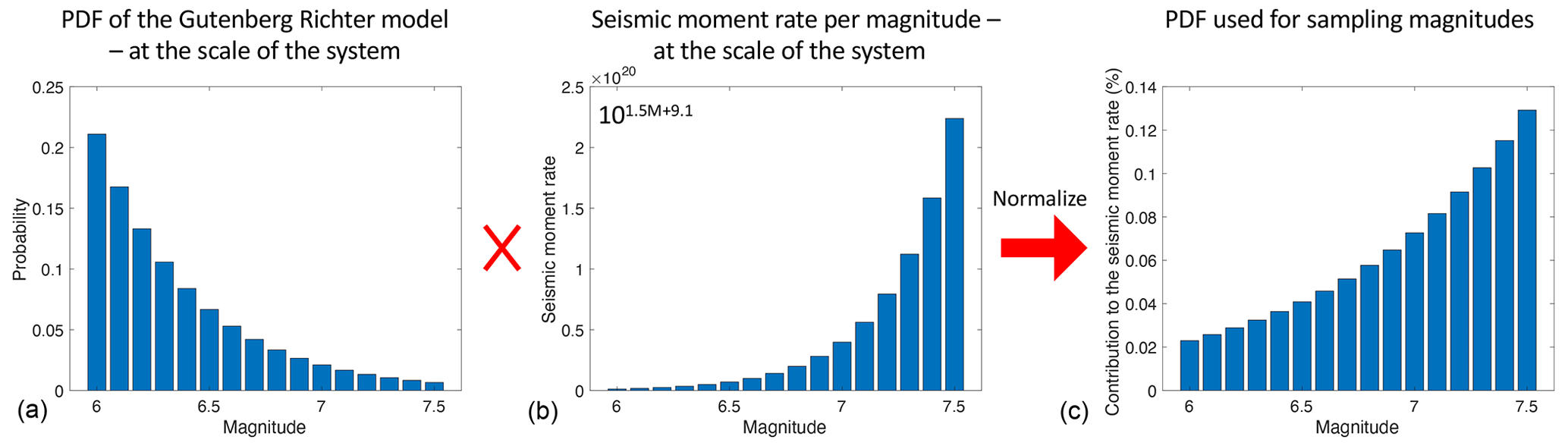
Figure A1 Steps for building the probability density function (PDF) used for sampling magnitudes in the SHERIFS iterative process (Chartier et al., 2017, 2019). The PDF of the Gutenberg–Richter model delivers probabilities of occurrence that decrease with increasing magnitude according to an exponential (a). These probabilities are multiplied by the corresponding moment rates (b), then normalized to obtain the final probability density function used to sample magnitudes in the iterative process (c).

Figure A2 Distribution of the section lengths, considering the 52 sections of the Levant fault system (Table 1).