High-resolution data assimilation for two maritime extreme weather events: a comparison between 3D-Var and EnKF

Populated coastal regions in the Mediterranean are known to be severely affected by extreme weather events. Generally, they are initiated over maritime regions, where a lack of in situ observations is present, hampering initial condition estimations and, hence, forecast accuracy. To face this problem, data assimilation (DA) is used to improve the estimation of initial conditions and their respective forecasts. Although comparisons between different DA methods have been performed at global scales, few studies have been conducted at high resolution, focusing on extreme weather events triggered over the sea and enhanced by complex topographic regions. In this study, we investigate the role of assimilating different types of conventional and remote sensing observations using the three-dimensional variational (3D-Var) approach and the ensemble Kalman filter (EnKF), which are the most common DA schemes used globally at national weather centers. To this aim, two different events are chosen because of both the different areas of occurrence and the triggering mechanisms. Both 3D-Var and EnKF are used at convection-permitting scales to improve the predictability of two high-impact coastal extreme weather episodes that were poorly predicted by numerical weather prediction models: (a) the heavy-precipitation event IOP13 and (b) the intense Mediterranean tropical-like cyclone Qendresa. Results show that EnKF and 3D-Var perform similarly for the IOP13 event for most of the verification metrics, although, looking at the receiver operating characteristic (ROC) curve and the area under the ROC curve (AUC) scores, EnKF clearly outperforms 3D-Var. However, the ensemble mean of EnKF is generally worse than that of 3D-Var for Qendresa, although some of the ensemble members of EnKF individually outperform 3D-Var, allowing for information to be gained on the physics of the event and hence the benefits of using an ensemble-based DA scheme.

1 Introduction

The Mediterranean Basin is recognized as one of the geographical regions most frequently affected by high-impact weather events in the world (Petterssen, 1956). The Mediterranean region has a natural disposition for these events because of its singular orographic features, which include having a relatively warm sea surrounded by complex terrain. This geographical configuration forces the warm and moist airflow to lift, favoring condensation and triggering convection. Hazardous weather events in this region, such as heavy precipitation (e.g., flash floods, snowstorms), cyclogenesis, and windstorms (e.g., squall lines, tornadic thunderstorms), cause huge economic losses, injuries, and fatalities in populated coastal regions (e.g., Romero et al., 1998; Llasat et al., 2010; Jansa et al., 2014; Flaounas et al., 2016; Pakalidou and Karacosta, 2018; Amengual et al., 2021). Since 1900, more than EUR 500 billion associated with total damages to property and over 1.3 million fatalities related to hydrometeorological disasters have been registered in the EM-DAT international disaster database (https://www.emdat.be/, last access: 29 August 2025). These effects underscore the critical need for accurate and rapid high-resolution weather forecasting systems, aimed at extending the lead time of severe weather warnings, thereby enabling the implementation of effective mitigation strategies to reduce fatalities and economic losses. However, while the accuracy of weather forecasting has significantly improved in recent years, with better representation of physical processes and dynamics, the accurate prediction of high-impact weather events in terms of their location, timing, and intensity remains a major challenge for the scientific community (Stensrud et al., 2009; Mass et al., 2002; Bryan and Rotunno, 2005; Yano et al., 2018; Torcasio et al., 2021). For this reason, improving the forecast of high-impact weather events is an imperative goal.

Deficiencies in the accurate prediction of the location (spatial and temporal), intensity, and phenomenology of extreme weather events are closely related to the accuracy of the initial conditions of the system (Wu et al., 2013). The initial conditions of the hazardous weather events affecting populated coastal regions are typically poorly estimated, mainly because these weather systems originate over the sea, where there is a lack of in situ observations. Enhanced representations of initial conditions are typically achieved by blending information from observations into numerical models through sophisticated data assimilation (DA) techniques (Kalnay, 2003), which accounts not only for the nominal values of the observations and the model, but also for their respective error statistics. DA has been widely used and applied to global numerical weather prediction (NWP) problems (e.g., Lorenc, 1981; Le Dimet and Talagrand, 1986; Rabier et al., 2000; Whitaker et al., 2008; Carrassi et al., 2018; Albergel et al., 2020). However, less attention has been paid to convective-scale NWP problems, especially those associated with small-scale convective phenomena initiated over regions with sparse observational data coverage, such as the extreme weather events affecting coastal regions in the Mediterranean Basin (Carrió and Homar, 2016; Amengual et al., 2017; Carrió et al., 2019; Lagasio et al., 2019; Amengual et al., 2021; Mazzarella et al., 2021; Torcasio et al., 2021; Capecchi et al., 2021). To improve forecasts of such extreme weather events, accurate high-resolution numerical weather models that solve convective-scale processes are required, along with dense observations at high spatial and temporal resolutions. These will provide accurate information regarding the convective systems themselves or their environmental conditions. One of the most important sources of convective-scale information are ground weather radars that provide 3D data related to storms at high spatial (order of hundreds of meters) and temporal (order of a few minutes) resolutions. In addition, weather radars provide thermodynamic and dynamic information on thunderstorms, which is crucial for understanding and forecasting convective structures. Due to the high spatio-temporal variability of convective structures, a rapid update cycle of the initial state (i.e., analysis) using weather radar observations is required to reduce errors and keep physical balances in the initial conditions. Several studies have shown the positive impact of forecasting severe weather events by assimilating weather radar information (e.g., Xiao and Sun, 2007; Lee et al., 2010; Wheatley et al., 2012; Yussouf et al., 2015; Carrió et al., 2019; Mazzarella et al., 2021).

During the last few decades, different DA algorithms have been developed with the aim of improving weather forecasts by making use of all available observations in the best possible way. In this context, most of the developed DA methods are based on exploiting Bayes' theorem (Lorenc, 1986) and making use of different types of approximations. Generally, DA algorithms can be classified into the following three Bayesian-based families: (a) variational DA (e.g., 3D-Var, Barker et al., 2004, or 4DVar, Huang et al., 2009); (b) ensemble-based DA, which is based on the ensemble Kalman filter (EnKF; Evensen, 1994); and (c) Monte Carlo DA methods. Variational DA minimizes a cost function to obtain the analysis (i.e., the best estimation of the initial conditions). More specifically, variational DA methods provide a (quasi-)optimal analysis based on an imperfect forecast (prior state or background), a set of imperfect observations, and their respective error statistics that are prescribed and assumed to be Gaussian, for simplicity. In addition, variational DA algorithms require a linearized and adjoint version of the numerical model, which can be very difficult to develop and maintain. This often involves the use of automatic differentiation tools or complex manual derivation, both of which are error-prone and time-consuming. On the other hand, ensemble-based DA algorithms do not require the use of linearized or adjoint versions of the model, and they do not use prescribed error statistics. Instead, they compute error statistics from an ensemble of forecasts, with the main property that these errors evolve in time as the system evolves. The Monte Carlo DA method allows for the assimilation of observations described with non-Gaussian errors. Particle filters (PFs; Van Leeuwen, 2009; Poterjoy, 2016) are a clear example of Monte Carlo DA algorithm. However, PFs are not well-suited for large multidimensional systems, such as the atmosphere, although a lot of improvements have been achieved recently. In the present study, we focus on the most widely used DA schemes typically used in major operational weather centers, namely the variational and ensemble-based DA schemes, leaving the Monte Carlo methods for future work.

Although variational DA schemes have been used in numerical weather prediction for many years (Courtier et al., 1994; Park and Županski, 2003; Rawlins et al., 2007), allowing for the assimilation of a wide range of different observations, they present a well-known limitation. This limitation is related to the use of a climatological background error covariance matrix to characterize error statistics, which is kept constant along the assimilation window, where the different observations are distributed at different times. This weakness is specifically linked to the 3D-Var method, which typically uses the National Meteorological Center (NMC) method (Parrish and Derber, 1992) to generate those static background error covariances using forecast differences over a period of time reasonably close to the event. The error statistics derived from such DA schemes are static, isotropic, and nearly homogenous, misrepresenting the true error statistics in space and time, which are inherently flow dependent, resulting in less accurate analysis. On the other hand, the EnKF DA scheme is designed to provide flow-dependent background error covariances. Some studies have shown the potential of EnKF to spread information from the observations in a flow-dependent manner in comparison with 3D-Var (Yang et al., 2009; Gao et al., 2018). On the other hand, 3D-Var techniques require fewer computational resources, and there is no need to build an ensemble, as in EnKF, or even simulate the model trajectory, as in 4D-Var. Therefore, assimilation with 3D-Var takes only a few tens of minutes, making this technique particularly suitable for operational purposes.

To resolve convective-scale (i.e., grid spacing of a few kilometers) physical processes associated with extreme weather phenomena, high-resolution numerical simulations and high-resolution initial conditions are required. This leads to performing computationally expensive high-resolution simulations, which poses a significant challenge by limiting the number of ensemble members that can be used in EnKF DA schemes, potentially hindering the estimation of the background error covariance matrix. Determining which DA method yields greater accuracy – 3D-Var using an ad hoc background error covariance matrix versus EnKF with a flow-dependent low-rank background error covariance derived from a finite ensemble – remains challenging under constrained computational resources.

Recent convective-scale DA studies have primarily focused on the mature stage of weather events (e.g., Tong and Xue, 2005; Fujita et al., 2007; Dowell et al., 2011; Jones et al., 2013; Wheatley et al., 2015; Jones et al., 2016; Gao et al., 2016; Ballard et al., 2016; Gustafsson et al., 2018; Carrió et al., 2019; Mazzarella et al., 2020; Yussouf et al., 2020; Federico et al., 2021; Wang et al., 2022). However, at this stage, the system is already well-developed and likely impacting the population, limiting the effectiveness of DA in terms of forecast lead time. In such cases, the potential for early warnings and mitigation actions is significantly reduced, as there is little time left to respond and minimize socio-economic impacts. Despite its potential benefits, only a handful of studies have explored the impact of DA using high-resolution numerical models in the developing stage (e.g., Carrió et al., 2019, 2022; Corrales et al., 2023), and even fewer have done so over data-sparse maritime regions, where early assimilation could be most valuable, providing advanced warnings and allowing decision-makers to act proactively. This study fills that gap by directly comparing two widely used DA techniques – 3D-Var and EnKF – in high-resolution, pre-convective assimilation experiments for two extreme weather events that initiated over the sea and affected populated coastal regions in the Mediterranean Basin. It is important to emphasize that this study does not aim to derive statistically significant conclusions. Instead, the main objective is to compare the performance of EnKF and 3D-Var in two distinct extreme weather events, each characterized by unique atmospheric conditions and observational limitations. The two extreme weather events selected for this study are (a) the heavy-rainfall episode IOP13, which affected coastal regions of Italy during October 2012 (Pichelli et al., 2017), and (b) the low-predictability Mediterranean tropical-like cyclone (medicane) Qendresa, which affected Sicily in November 2014 (Pytharoulis et al., 2017; Pytharoulis, 2018; Cioni et al., 2018; Di Muzio et al., 2019).

Overall, this study aims to do the following:

• a.

  assess the impact of 3D-Var in comparison with the EnKF system in predicting small-scale extreme weather events initiated over maritime regions with a lack of in situ observations

• b.

  compare the forecast impact from assimilating in situ conventional observations versus high-spatial- and high-temporal-resolution data from remote sensing instruments

• c.

  provide a quantitative assessment between the different DA schemes using several statistical verification methods.

This paper is organized as follows. Section 2 briefly describes the meteorological characteristics of the two events used for comparing the impact of 3D-Var and EnKF. In Sect. 3 the observational dataset assimilated by the different DA methods is presented. Section 4 briefly explains the main characteristics of the two DA algorithms that are used in this study. The numerical model configuration and the design of the different experiments for the two different case studies are then described in Sects. 5 and 6, respectively. Section 7 describes the verification methods used in this study. Results of the different numerical experiments for both meteorological situations are summarized in Sect. 8. Finally, conclusions are presented in Sect. 9.

2 Brief description of case studies

Two different extreme weather systems, occurring in the Mediterranean region and affecting populated coastal regions, are considered in this study. The first extreme weather event was associated with heavy rainfall that affected central and northern Italy during October 2012 (IOP13), while the second extreme weather event was associated with Medicane Qendresa, affecting southern Sicily, Lampedusa, Pantelleria, and Malta during November 2014. Both systems were poorly forecasted, making them perfect candidates for this intercomparison study to assess the impact of data assimilation techniques.

2.1 The IOP13 heavy-precipitation episode

IOP13 occurred during the first special observation period (SOP1) of the international Hydrological cycle in the Mediterranean Experiment (HyMeX) project (Drobinski et al., 2014), which was mainly designed to better understand heavy-rainfall and flash flooding episodes occurring in the Mediterranean region. The heavy-precipitation IOP13 event took place between 14 and 16 October 2012, and it was characterized by a frontal precipitation system associated with a deep upper-level trough extending from northern France towards northern Spain (Fig. 1). It initially affected coastal areas in southern France, and afterward it also affected the northern and central parts of Italy. During 15 October, the Italian rain gauge network registered 24 h accumulated precipitation with peaks reaching 60 mm in central Italy, 160 mm in northeastern Italy, and 120 mm in Liguria and Tuscany. During the night of 14 October, a cold front affected the western Mediterranean region, and during 15 October, the system rapidly moved from France to Italy, advecting low-level moisture towards the western coast of Italy and Corsica, destabilizing the atmosphere and favoring deep moist convective activity. More details on the synoptic situation and observational data collected during IOP13 can be found in Ferretti et al. (2014).

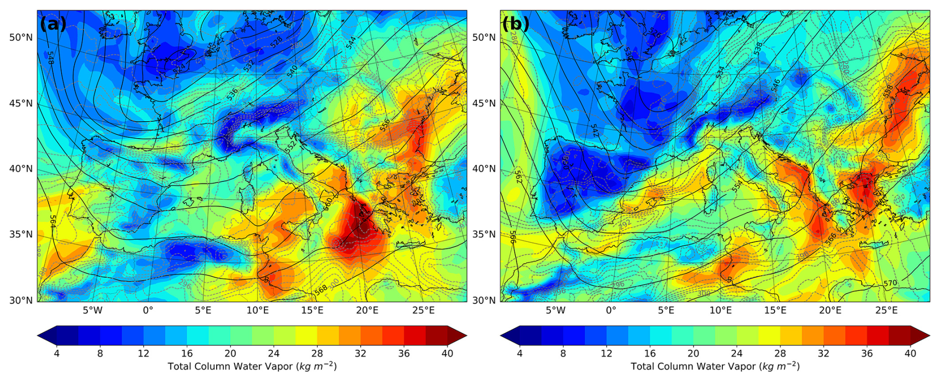
Figure 1 IOP13 ERA5 analyses: 500 hPa geopotential height (solid black lines), 925 hPa temperature (dashed grey lines), and total column water vapor (color-shaded areas) at (a) 12:00 UTC on 14 October and (b) 00:00 UTC on 15 October 2012.

2.2 The Qendresa tropical-like cyclone episode

Among the wide spectrum of maritime extreme weather events, tropical-like Mediterranean cyclones, a.k.a. medicanes (Emanuel, 2005), draw particular attention to the community mainly because they share similar morphological characteristics to tropical cyclones. Given their tendency to impact densely populated and economically critical areas around the Mediterranean Basin, enhancing the accuracy and reliability of medicane forecasts has become an urgent priority. Here, we focus on the 7 October 2014 medicane (Qendresa; Cioni et al., 2018) that affected the islands of Lampedusa, Pantelleria, and Malta and the eastern coast of Sicily. This event was recognized by the community for its limited predictability (Carrió et al., 2017), making it a compelling case study for investigating the performance of the 3D-Var and EnKF DA methods. In situ observations located in Malta's airport registered gust wind values exceeding 42.7 m s⁻¹ and a sudden and deep pressure drop greater than 20 hPa in 6 h. Satellite imagery during its mature phase showed a well-defined cloud-free eye surrounded by axisymmetric convective activity, which resembles the morphological properties of classic tropical cyclones.

A deep upper-level trough associated with a cyclonic flow at mid-levels characterized the synoptic situation in the western Mediterranean from 5 to 8 November 2014. The upper-level trough was associated with an intense potential vorticity (PV) streamer extending from northern Europe to southern Algeria, and the cyclonic flow at mid-levels was dominated by a strong ridge over the Atlantic and a deep trough moving along western Europe. Late on 7 November, the upper-level trough became negatively tilted, evolving into a deep upper-level cutoff low, and the PV streamer disconnected from the northern nucleus (Fig. 2). A small well-defined spiral-to-circular cloud shape formed just south of Sicily and evolved east-northeastward, reaching its maximum intensity over Malta, at midday. Finally, the cyclonic system dissipated as it crossed the Catania (eastern) coast of Sicily. More details on the synoptic situation and observational data collected during this event can be found in Carrió et al. (2017).

Figure 2 Qendresa ERA5 analyses: 500 hPa geopotential height (solid black lines), 500 hPa temperature (dashed grey lines), and 300 hPa potential vorticity (color-shaded areas) at (a) 00:00 UTC on 7 November and (b) 00:00 UTC on 8 November 2014.

3 Observation description

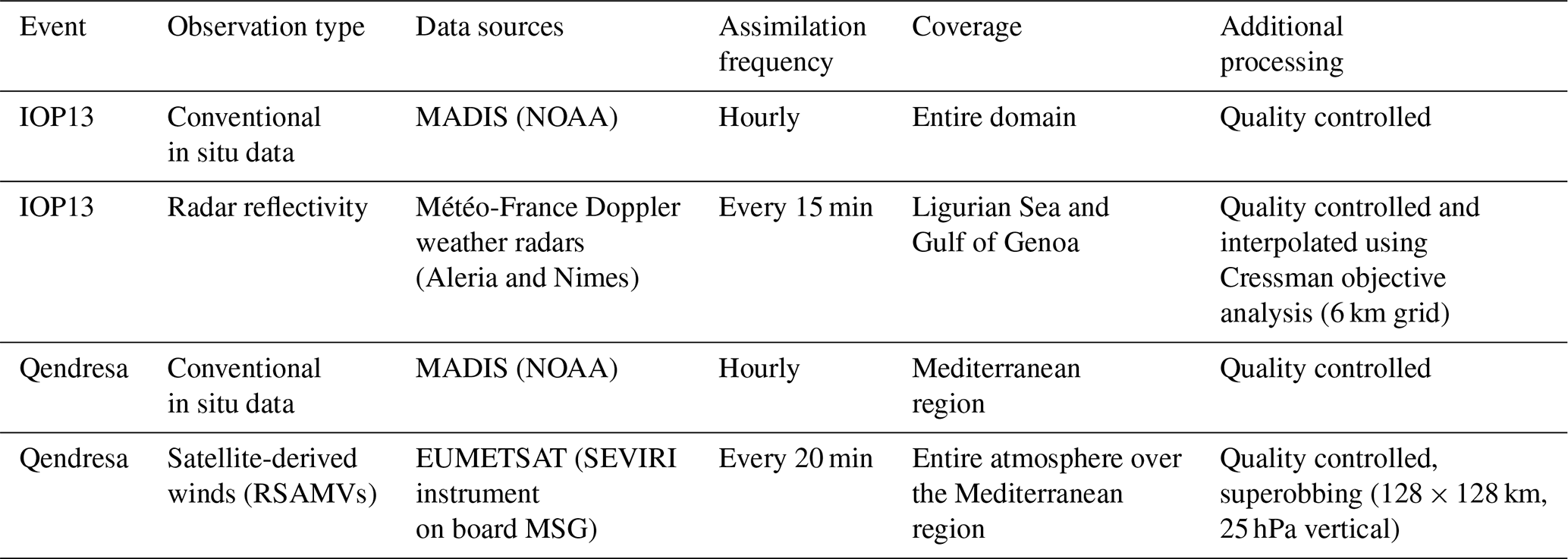
In this study, a combination of remote sensing and in situ observations was assimilated for both case studies. Specifically, the following three types of observations were assimilated: (a) conventional in situ data from surface meteorological stations, maritime buoys, rawinsondes, and aircraft measurements; (b) high temporal and spatial reflectivity data from two Doppler weather radars; and (c) satellite-derived 3D wind speed and direction data. A summary of the assimilated observations, including their data sources, assimilation frequency, coverage, and additional processing, is provided in Table 1.

Table 1 Summary of assimilated observations for each case study, including observation type, data sources, assimilation frequency, spatial coverage, and additional processing details.

3.1 IOP13 observations

For IOP13, we assimilated both in situ conventional data and remote sensing observations from two Doppler weather radars. While Italy has a dense national network of radar and in situ stations, most of these datasets are not publicly available. To ensure reproducibility and accessibility, we exclusively used freely available data. For radar observations, we assimilated data from the only two radars providing coverage over the maritime region where the event initiated. Specifically, we used data from (a) the Aleria radar (42.129° N, 9.496° E; 63 m a.s.l.), located on Corsica, and (b) the Nimes radar (43.806° N, 4.502° E; 76 m a.s.l.), located in southern France (Fig. 3a). These two Météo-France polarimetric S-band Doppler weather radars, strategically positioned, ensure good spatial coverage over the Ligurian Sea, the area where triggering and intensification of deep convection occurred, and provide key information about the 3D structure of the convective systems at high spatial and temporal resolutions. The Aleria and Nimes radars perform five and nine elevation scans every 5 min, respectively, and their data are available on HyMeX's official website (see https://www.hymex.org/, last access: 9 December 2024). Specifically, the Aleria radar provides data at five elevation angles: 0.57, 0.96, 1.36, 3.16, and 4.57°, with a mean frequency of 2.8 GHz. In comparison, the Nimes radar provides data at nine elevation angles: 0.58, 1.17, 1.78, 2.38, 3.49, 4.99, 6.5, 7.99, and 89.97°, also at the same frequency. It is worth mentioning that Aleria and Nimes radar reflectivity data are provided by the Météo-France operational radar network and undergo rigorous data quality control. This ensures that common radar error sources, such as signal attenuation, ground clutter, or beam blocking, are meticulously identified and corrected. Radial velocity from the Aleria and Nimes Doppler radars was also available, but because of the low reliability of the data (not quality controlled properly), it was not used in this study. Additionally, conventional in situ observations were obtained from the National Oceanic and Atmospheric Administration (NOAA) Meteorological Assimilation Data Ingest System (MADIS), a global dataset that provides high-quality, quality-controlled meteorological observations. In particular, we assimilated pressure, temperature, humidity, and horizontal wind speed and direction from in situ instruments, such as METARs, maritime buoys, rawinsondes, and aircraft (Fig. 3a).

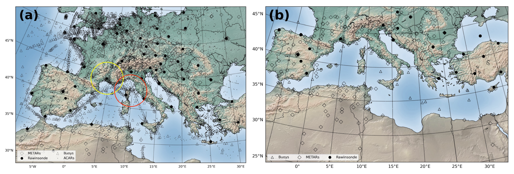
Figure 3 (a) IOP13 episode: spatial distribution of in situ observations (gray and black markers) assimilated on the parent numerical domain during the 24 h assimilation window from 00:00 UTC on 14 October to 00:00 UTC on 15 October 2012. Doppler weather radars located at Nimes and Aleria and their coverage range, depicted in yellow and red circles, respectively. (b) Qendresa episode: spatial distribution of in situ observations assimilated on an hourly basis during the 12 h assimilation window from 12:00 UTC on 6 November to 00:00 UTC on 7 November 2014. Publisher's remark: please note that the above figure contains disputed territories.

Overall, the following observations were assimilated for this event:

• Conventional in situ data were assimilated hourly over the entire model domain (Fig. 3a).

• Reflectivity data from the Aleria and Nimes weather radars were assimilated every 15 min (Fig. 3a).

The high spatial resolution of the reflectivity data poses significant challenges for their direct assimilation, potentially leading to detrimental analysis related to signal aliasing and the violation of the uncorrelated observational error assumptions used in the derivation of the 3D-Var and EnKF analysis equations. To mitigate the adverse effects associated with these issues, the Cressman objective analysis technique (Cressman, 1959) was used to interpolate raw radar observations to a regularly spaced 6 km horizontal grid, as suggested by previous work (i.e., Wheatley et al., 2015; Yussouf et al., 2015). It is important to note that reflectivity observations are typically obtained in polar coordinates, a prerequisite step before applying the Cressman interpolation, which involves converting them to a Cartesian coordinate system. We performed several sensitivity tests using different grid space resolutions (e.g., 3, 6, 9 km), and we found that using a 6 km grid space produces the best analysis. To reduce spurious convective signals and remove excessive humidity, the null-echo option, which allows for assimilation of no precipitation echoes, was adopted in the 3D-Var experiment.

3.2 Qendresa observations

For the Qendresa event, two different observational sources were publicly available: (a) conventional in situ observations and (b) satellite-derived observations. Conventional in situ observations were obtained from the MADIS database. However, only observations from buoys, METAR, and rawinsonde were used for this case. It is essential to highlight that observation gaps persist across large areas of the region, particularly over the sea (Fig. 3b), where Qendresa initiated and evolved. As for IOP13, we were interested in Doppler weather radar data to enhance the intensity and trajectory forecasts of Qendresa. Unfortunately, Doppler weather radars were not publicly available in the neighborhood of the region where Qendresa initiated and evolved. Instead, we used an alternative high-resolution data source, so-called rapid-scan atmospheric motion vectors (RSAMVs; Velden et al., 2017). This dataset provides 3D wind information throughout the entire atmosphere (both speed and direction) at high spatial and temporal resolutions (i.e., every 20 min). These observations were particularly valuable for capturing wind field structures over the sea, where conventional observations were sparse or unavailable. This satellite product is obtained using the Spinning Enhanced Visible and Infrared Imager (SEVIRI) instrument on board the Meteosat Second Generation (MSG) satellite, which has a scanning frequency as low as 5 min. The final product is indeed obtained by averaging four consecutive images.

Hence, the following observations were assimilated for this event:

• Conventional in situ data from buoys, METAR, and rawinsonde for the entire Mediterranean region were assimilated hourly.

• Wind speed and direction from rapid-scan atmospheric motion vectors for the entire atmosphere at high spatial and temporal resolutions were assimilated every 20 min.

Recent studies have shown that upper-level dynamics played a key role in the genesis and the development of Qendresa (Carrió et al., 2017; Carrió et al., 2022), so the assimilation of RSAMVs is expected to significantly improve its predictability. Here, the infrared channel from RSAMVs (10.8 µm), which contains information throughout the entire atmosphere, was selected to be assimilated (Fig. 4). However, before assimilating RSAMVs, a quality control check to reject non-physical and outlier observations, which could deteriorate the quality of the analysis and the successive forecast, was applied. In addition, to minimize the effect of having spatially correlated observation errors associated with high-density observations, the superobbing technique, consisting of reducing data density by spatially averaging observations within a predefined prism, is applied (i.e., Pu et al., 2008; Romine et al., 2013; Honda et al., 2018). Based on the most accurate analysis obtained by multiple sensitivity experiments (not shown) for Qendresa, the RSAMV data are thinned using a prism with a horizontal resolution of 128 × 128 km² and 25 hPa in the vertical.

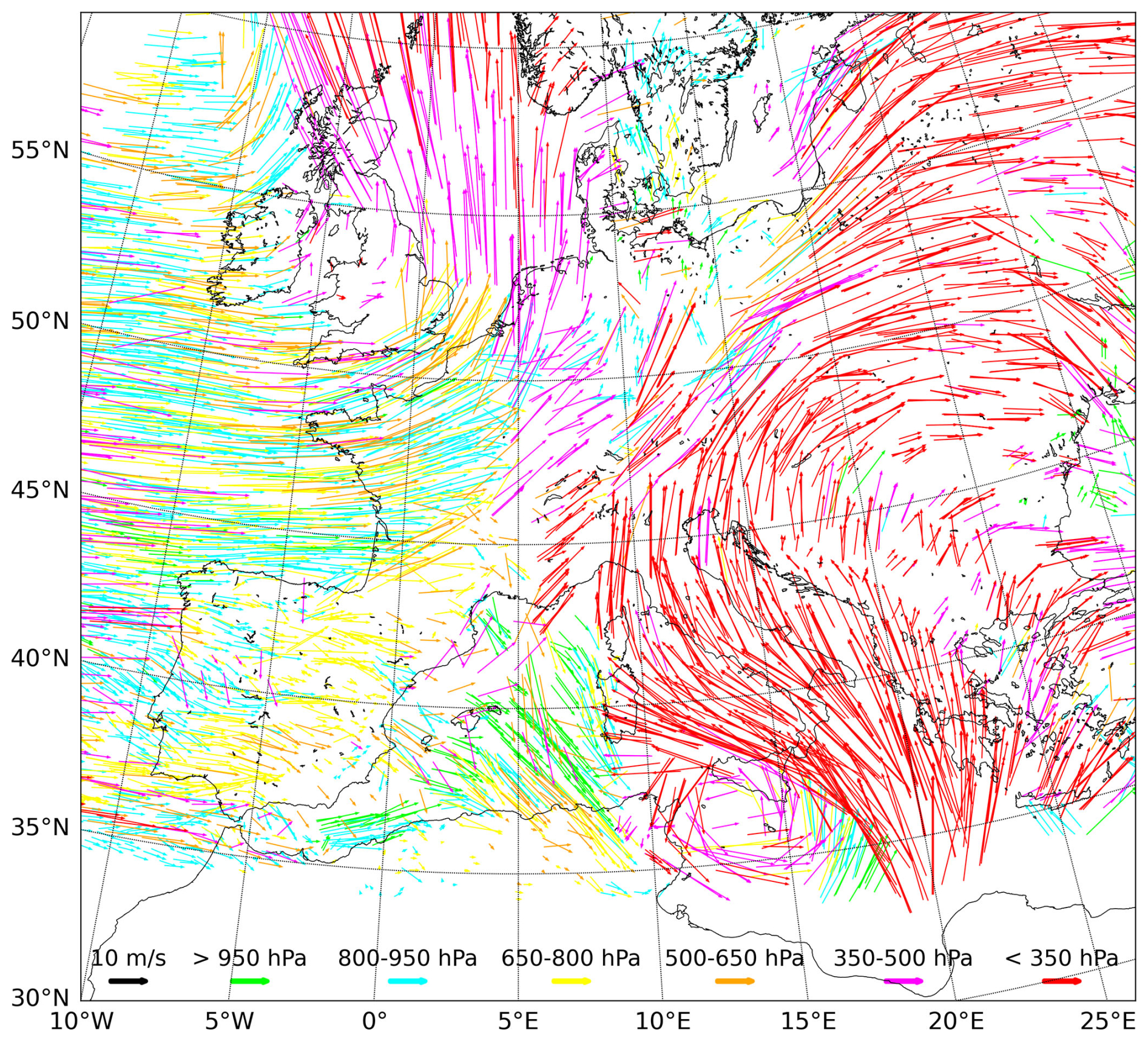
Figure 4 Raw EUMETSAT RSAMV observations depicted at different vertical levels from the 10.8 µm infrared channel at 12:00 UTC on 7 November 2014 over the Mediterranean region. Wind information is only valid at the center of the wind vectors.

Observations from aircraft (i.e., ACARS) were not assimilated in this case because preliminary assimilation tests indicated a worsening of the results, which led to a poorer estimation of the atmospheric state. Buoy, METAR, and rawinsonde observations covering the entire Mediterranean region were assimilated hourly.

Finally, the observational errors used for the assimilation of the observations associated with both IOP13 and Qendresa are motivated by Table 3 in Romine et al. (2013), with the following minor changes: METAR altimeter (1.5 hPa), marine altimeter (1.20 hPa), METAR and marine temperature (1.75 K), and RSAMV wind observations (1.4 m s⁻¹). These minor changes are found to provide better data assimilation analysis for the IOP13 and Qendresa extreme weather events in the Mediterranean region. The remaining observation errors are the same as the ones in Romine et al. (2013).

4 Data assimilation schemes

In the present study, two widely used data assimilation algorithms are used to improve the forecast of extreme weather events that initiated and developed over poorly observed maritime regions and affected densely populated coastal areas. We refer to the ensemble adjustment Kalman filter and the 3D-Var data assimilation schemes, which are briefly described below.

4.1 The ensemble adjustment Kalman filter (EnKF)

The ensemble adjustment Kalman filter (EAKF; Anderson, 2001), which is implemented in the Data Assimilation Research Testbed (DART) facility (http://www.image.ucar.edu/DAReS/DART/, last access: 24 August 2024), is used in this study as the formerly mentioned ensemble-based data assimilation technique. The EAKF provides an optimal estimation, in a least squares error sense, of the true probability distribution of the state of the atmosphere by merging two main sources of information: (a) the available observations and (b) an ensemble of forecasts (a.k.a. background) valid at the analysis time. In particular, the EAKF assimilates the observations serially. This means that the analysis ensemble obtained by the EAKF after the assimilation of the first observation at a given time is then used as the background for the next observation at the same analysis time. This is done recursively until all the observations valid at the same analysis time are finally assimilated.

Ensemble covariances used in real case studies, where only a limited number of ensemble members is feasible, suffer from sampling error, resulting in the generation of spurious correlations that hamper the analysis (Hacker et al., 2007). The detrimental effects of these spurious correlations are mitigated by employing covariance localization functions that go to zero as the distance between the assimilated observation and the grid model point where the analysis occurs increases (Houtekamer and Mitchell, 1998). In our case, a fifth-order piecewise rational Gaussian localization function is used (Gaspari and Cohn, 1999). For this study, after several sensitivity simulations, it was found that using a half radius¹ of 230 km in the horizontal and a half radius of 4 km in the vertical for the horizontal and vertical localizations, respectively, results in the best performance of the DA scheme.

Assimilating observations inherently reduces analysis variance in both variational and Kalman filter frameworks. Small ensemble sizes tend to overly collapse the ensemble spread (Anderson and Anderson, 1999). To mitigate this under dispersion and maintain realistic ensemble variance, a spatially varying adaptive inflation technique (Anderson and Collins, 2007; Anderson et al., 2009) is applied to the prior ensemble before assimilating the observations. This adaptive inflation technique increases the spread of the ensemble without changing the mean. The inflation value has a probability density distribution described by a mean and a standard deviation. In this study, it was determined that initializing the mean value of inflation at 1.0 and using a standard deviation of 0.6 yield the best performance of the DA scheme.

4.2 Three-dimensional variational (3D-Var) data assimilation

The 3D-Var technique, implemented in the Weather Research and Forecasting data assimilation (WRFDA) system (Barker et al., 2004), is adopted for the numerical simulations. 3D-Var aims to seek the best estimate of initial conditions through the iterative minimization of a cost function:

$$\begin{array}{rl}J\left(\mathit{x}\right)={\displaystyle \frac{\mathrm{1}}{\mathrm{2}}}& \mathit{\{}{\left(\mathit{x}-{\mathit{x}}_{\mathrm{b}}\right)}^T{\mathbf{B}}^{-\mathrm{1}}\left(\mathit{x}-{\mathit{x}}_{\mathrm{b}}\right)\\ & +{\left({\mathit{y}}_{\mathrm{o}}-H\left(\mathit{x}\right)\right)}^T{\mathbf{R}}^{-\mathrm{1}}\left({\mathit{y}}_{\mathrm{o}}-H\left(\mathit{x}\right)\right)\mathit{\}},\end{array}$$

where B and R are the background and observation error matrices, respectively; x is the state vector; y_o is the observation; x_b is the first guess; and H is the forward (non-linear) operator that converts data from model space to observation space.

The solution of the above cost function J consists of finding a state x_a (analysis), which minimizes the distance between the observations and the background field. However, in a model with 10⁶ degrees of freedom, the direct solution is computationally expensive. To reduce the complexity and calculate B⁻¹ more efficiently, a preconditioning is applied by transforming the control variables – pseudo-relative humidity, temperature, u, v, and surface pressure – to x−x_b = Uv, where v is the control variable and U the transformation operator.

The background error covariance matrix B plays a key role in the assimilation process by weighing and smoothing the information from observations and by ensuring a proper balance between the analysis fields. The National Meteorological Center (NMC) method (Parrish and Derber, 1992) was used to model the B matrix. This method evaluates the differences between two short-term forecasts valid at the same time but with different lead times, 12 and 24 h, respectively, to generate the forecast error covariance matrix B. In this study, we build the 3D-Var B matrix over a 2-week period, in line with our operational experience running 3D-Var and previous demonstrations of its benefits (Hung et al., 2023; Fitzpatrick et al., 2007; Mazzarella et al., 2020, 2021). To enhance B's quality despite this relatively short sampling window, we activate the CV7 option in WRFDA. This option uses empirical orthogonal functions (EOFs) to represent vertical covariances instead of the traditional recursive filter, which has proven to be particularly beneficial for radar reflectivity assimilation and subsequent precipitation forecast improvements (Wang et al., 2013; Li et al., 2016; Shen et al., 2022; Ferrer Hernández et al., 2022). In our configuration, the CV7 control variables (i.e., u, v, temperature, pseudo-relative humidity, and surface pressure) are defined in EOF space, ensuring a compact yet accurate representation of error structures. We use the CV7 option to generate the B matrix for both case studies. In addition, the weak penalty constraint (WPEC) option (Li et al., 2015) in WRFDA has also been activated to further improve the balance between the wind and thermodynamic state variables, enforcing the quasi-gradient balance on the analysis field.

5 Model set-up

The mesoscale Advanced Research Weather Research and Forecasting (WRF) model (Skamarock et al., 2008) version 3.7 is used in this study. WRF solves a fully compressible and non-hydrostatic set of equations, using an η terrain-following hydrostatic pressure vertical coordinate. The Arakawa C-grid staggering scheme and a third-order Runge–Kutta time integration are used to improve the precision of the numerical solutions. Because the IOP13 and Qendresa episodes took place in different locations and with different conditions, two different model configurations were used. For the IOP13 episode, a one-way-nested model configuration with the parent domain centered over the western Mediterranean Sea, covering central Europe and northern Africa with a horizontal grid resolution of 15 km (168 × 247), and a nested domain centered over the Gulf of Genoa with a horizontal grid resolution of 3 km (250 × 250) were used (Fig. 5a). A total of 51 vertical model levels from the surface to 50 hPa were used, with a higher density of levels in the lower part of the atmosphere than in the upper part for both domains. For Qendresa, a one-way-nested model configuration is also used, but now the parent domain is centered over the central Mediterranean Sea, covering most of the European region and the northern part of Africa (Fig. 5b), using a horizontal grid resolution of 15 km (245 × 245). The nested domain is centered over Sicily (southern Italy) using a grid resolution of 3 km (253 × 253). Both numerical domains use 51 terrain-following η levels up to 50 hPa, as in the IOP13 case.

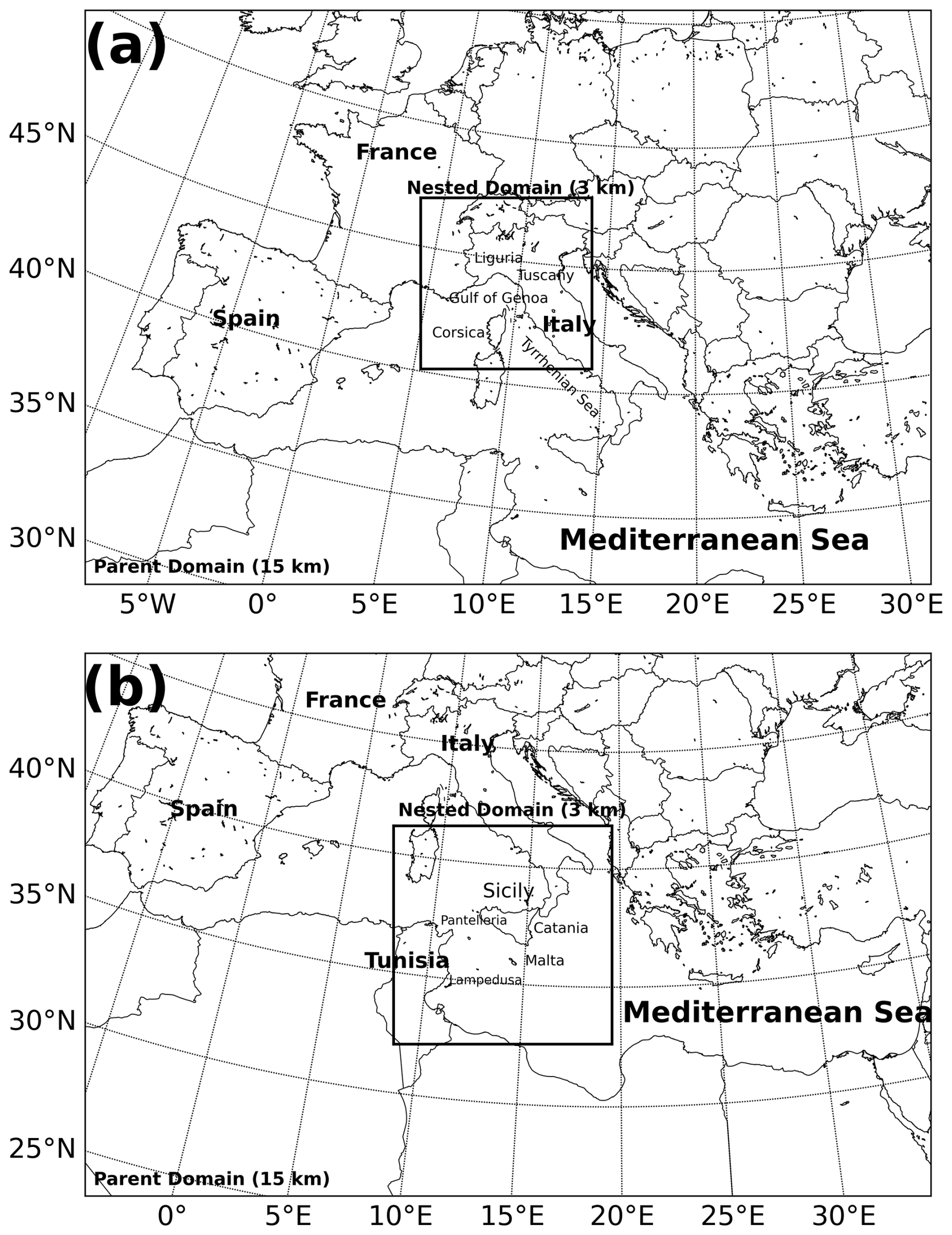
Figure 5 Mesoscale and storm-scale numerical domains used in this study for the (a) IOP13 and (b) Qendresa episodes, respectively. Publisher's remark: please note that the above figure contains disputed territories.

For the EnKF DA experiments, initial and boundary conditions used to perform the simulations associated with IOP13 were obtained from the European Centre for Medium-Range Weather Forecasts Global Ensemble Prediction System (EPS-ECMWF), which stored meteorological fields using a horizontal and vertical spectral triangular truncation of T639L62 (i.e., ∼ 32 km grid resolution in the horizontal). In particular, EPS-ECMWF provides 51 different initial and boundary conditions from 50 perturbed ensemble members and a control simulation. However, due to unfeasible computational resources required to run our numerical simulations at high resolution, here we use an ensemble consisting of 36 members. This configuration is analogous to that used at the internationally prestigious National Oceanic and Atmospheric Administration National (NOAA) Severe Storms Laboratory (NSSL) in Norman (Oklahoma, USA) to improve predictability of tornadoes. To obtain the desired 36-member ensemble, a principal component analysis and k-means clustering technique were used together to select the 36 ensemble members from EPS-ECMWF, showing more dispersion over the entire numerical domain (see Garcies and Homar, 2009, and Carrió and Homar, 2016, for more details using these techniques). To perform Qendresa DA simulations, the initial and boundary conditions are obtained following the same methodology explained above for the IOP13 case, i.e., using an ensemble of 36 members obtained from EPS-ECMWF. On the other hand, the initial and boundary conditions for 3D-Var simulations are provided by the Integrated Forecasting System (IFS) global model from ECMWF, with a spatial resolution of 0.1° × 0.1° and updated every 3 h.

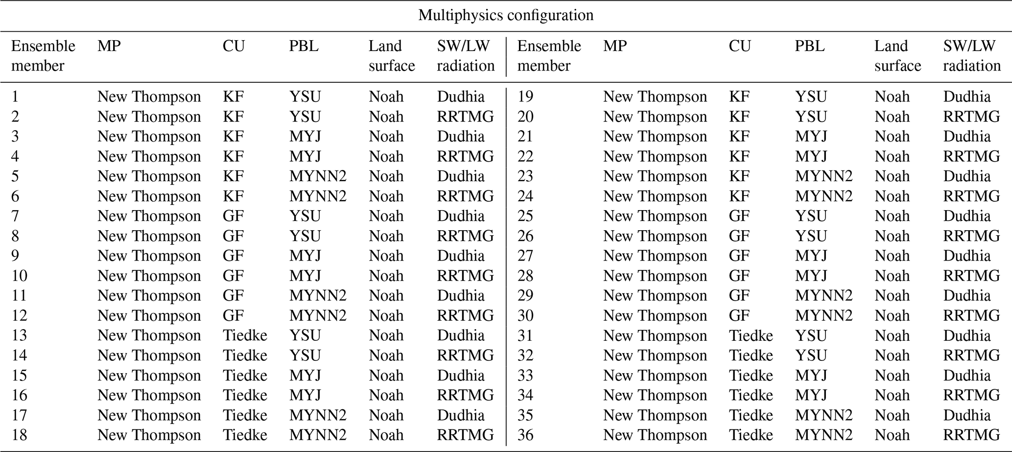
To estimate the uncertainties in WRF, which is necessary information for EnKF, a multiphysics ensemble is built for both the IOP13 and the Qendresa events (e.g., Stensrud et al., 2000; Wheatley et al., 2012), where each ensemble member gets a different set of parameterizations (see Table 2). In particular, the diversity in our ensemble consists of (a) two short- and longwave radiation schemes (Dudhia: Dudhia, 1989, and RRTMG: Iacono et al., 2008), (b) three cumulus parameterization schemes (Kain–Fritsch, KF: Kain and Fritsch, 1990; Kain, 2004; Tiedtke: Tiedtke, 1989; and Grell–Freitas, GF: Grell and Freitas, 2014), and (c) three planetary boundary layer schemes (Yonsei University, YSU: Hong et al., 2006; Mellor–Yamada–Janjić, MYJ: Janjić, 1990; and Mellor–Yamada–Nakanishi–Niino level 2.5, MYNN2: Nakanishi and Niino, 2006, 2009). Two widely used physics parameterizations are adopted for the microphysical processes and land surface interactions, the New Thompson (Thompson et al., 2008) and Noah (Tewari et al., 2004) schemes, respectively. Note that the above-mentioned physical parameterizations are used for both the large-scale ensemble in the parent domain and the storm-scale ensemble in the nested domain, except for the cumulus parameterization, which is only applied in the parent domain ensemble. On the other hand, for the WRF deterministic simulation using 3D-Var, the microphysical processes are parameterized by using the New Thompson scheme, while the YSU scheme is adopted for PBL. Long- and shortwave radiation is considered through the RRTMG and Dudhia schemes, respectively, while the Kain–Fritsch scheme is used for convection, except for the inner domain, where it is explicitly resolved.

Table 2 Multiphysics parameterizations used to generate the 36-member ensemble for the EnKF experiments in the IOP13 and Qendresa episodes. PBL, SW, and LW stand for planetary boundary layer, shortwave, and longwave, respectively.

6 Design of IOP13 and Qendresa experiments

To quantify the benefits of assimilating different observation types with the 3D-Var and EnKF DA schemes, a suite of numerical experiments is designed. First, a reference experiment without any data assimilation (NODA), using the same model configuration employed for the WRF experiments performed using 3D-Var, is carried out at the regional scales considered in this study. Building on this, several numerical experiments, each differing only in the type of observations assimilated to isolate and compare their impacts on forecast skill, are performed. Only conventional in situ observations are assimilated using 3D-Var and EnKF for the first set of experiments (SYN). All available observations (i.e., conventional, radar-based, and satellite-derived data) are assimilated using both 3D-Var and EnKF for the second type of experiments (CNTRL). The comparison between these numerical experiments will provide information on which DA scheme and observation perform better for these weather events. The DA experiments mainly consist of two phases: the first one is related to the data assimilation procedure, where different types of observations are assimilated by the 3D-Var and EnKF DA schemes, and the second phase is associated with the free model run initialized using the initial conditions obtained during the first phase. The total forecast time is 24 and 36 h for IOP13 and Qendresa, respectively. For IOP13, a further simulation lasting 6 h from 18:00 UTC on 13 October to 00:00 UTC on 14 October 2012 (Carrió et al., 2019) is performed (Fig. 6) to reduce spin-up problems related to the direct downscaling from the global ECMWF analysis (32 km grid resolution) to the WRF parent domain used in our simulations (16 km grid resolution). This procedure improved the DA for IOP13, but it had a small impact for Qendresa.

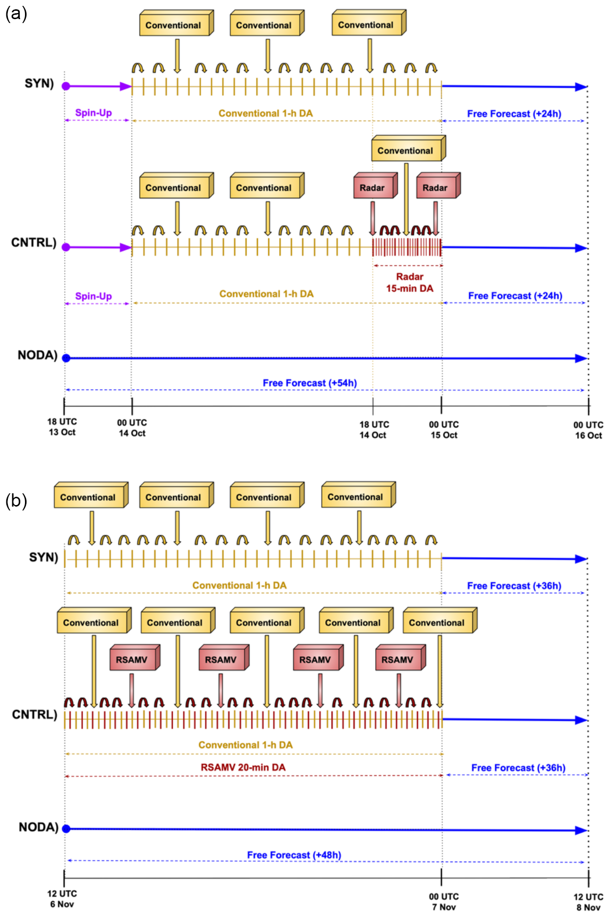
Figure 6 Schematic representation of the main numerical experiments performed in this study for the (a) IOP13 and (b) Qendresa episodes. SYN, CNTRL, and NODA experiments are illustrated for each case, highlighting their respective configurations and assimilation strategies.

Therefore, the following model simulations were performed:

• no data assimilation (NODA)

• only conventional in situ observations using 3D-Var and EnKF (SYN)

• all available observations (i.e., conventional, radar-based, and satellite-derived data) using both 3D-Var and EnKF (CNTRL).

The comparison between the DA experiments and NODA allows us to assess the impact of the DA procedure. On the other hand, the comparison between SYN and CNTRL allows for the role of radar and/or satellite data to be assessed, especially for the events that originated in the area where observations are not available. Moreover, the assimilation of the radar and/or satellite produces important information on the triggering phase of both events developing over the sea.

6.1 CNTRL experiments

For IOP13, the CNTRL experiment is designed to assimilate both in situ conventional and reflectivity observations from the Aleria and Nimes Doppler weather radars. The assimilation of the reflectivity is expected to improve the forecast of this event by significantly improving the initial conditions over the sea, where convective activity initiated and evolved into deep convection, affecting the populated coastal areas of Italy. As briefly described in the previous section, this experiment consists of three stages: (1) the spin-up of the storm-scale domain is accounted for by running the WRF model during 6 h from 18:00 UTC on 13 October to 00:00 UTC on 14 October 2012 (note that for the 3D-Var experiment, the spin-up is accounted for by just initializing WRF with the deterministic analysis from the IFS ECMWF; however, for the EnKF counterpart, the spin-up is accounted for by initializing the 36-member ensemble at 18:00 UTC on 13 October); (2) in situ conventional observations were assimilated hourly during 24 h from 00:00 UTC on 14 October to 00:00 UTC on 15 October, while reflectivity observations were assimilated using a rapid-update assimilation cycle every 15 min during a period of 6 h, from 18:00 UTC on 14 October to 00:00 UTC on 15 October (Fig. 6); and (3) a 24 h ensemble (deterministic) forecast until 00:00 UTC on 16 October, using the recently obtained initial conditions, was performed by EnKF (3D-Var).

For the Qendresa episode, the CNTRL experiment is designed to assimilate both in situ conventional and RSAMV observations. The assimilation of RSAMV observations is expected to improve the representation of the atmospheric circulation at upper levels, whereas the assimilation of surface conventional observations is expected to enhance the representation at low levels. The Qendresa CNTRL experiment consists of two main phases: (1) in situ conventional and satellite-derived RSAMV observations are assimilated hourly and at 20 min intervals, respectively, during a 12 h period from 12:00 UTC on 6 November to 00:00 UTC on 7 November 2014 to end up with the last analysis at the end of the assimilation window (i.e., 00:00 UTC on 7 November), and (2) a free 36 h ensemble (deterministic) forecast is performed by EnKF (3D-Var) from 00:00 UTC on 7 November to 12:00 UTC on 8 November 2014 (Fig. 6e).

6.2 SYN experiments

For IOP13, the SYN experiment assesses the impact of in situ conventional observations, which are crucial for characterizing mesoscale atmospheric circulation. Analogous to the CNTRL, SYN follows the same three phases, but in the second phase only the hourly in situ conventional observations from 00:00 UTC on 14 October to 00:00 UTC on 15 October 2012 are assimilated. The analysis obtained from the assimilation stage is used as initial conditions for running the free forecast for 24 h in the third phase (Fig. 6).

Similarly, for Qendresa, only in situ conventional observations are assimilated hourly in the SYN experiment for 12 h, from 12:00 UTC on 6 November to 00:00 UTC on 7 November 2014 (Fig. 6).

6.3 NODA experiments

For IOP13, the NODA experiment is a direct downscaling from EPS-ECMWF boundary and initial conditions valid at 18:00 UTC on 13 October to 00:00 UTC on 16 October 2012 (Fig. 6). The comparison between NODA, CNTRL, and SYN provides us with valuable information on the impact of assimilating different sources of observations.

For Qendresa, the NODA experiment is simply a direct downscaling of 36 h from EPS-ECMWF at 00:00 UTC on 7 November to 12:00 UTC on 8 November 2014 (Fig. 6). Here again, it is important to note that the choice of starting NODA at 00:00 UTC on 7 November instead of starting at 12:00 UTC on 6 November was made intentionally to extract general conclusions possibly applicable to an operational framework.

7 Verification methods

To quantitatively evaluate the performance of EnKF and 3D-Var and their impact on the short-term forecast of these two extreme weather events, various verification scores are used. Given the different natures of the weather phenomena associated with these episodes, the selection of verification scores is tailored specifically to each event. For the IOP13 heavy-precipitation event (Fig. 7a), model verification was performed using the observed accumulated precipitation field over different time windows (e.g., 3, 6, and 9 h). More specifically, the accumulated precipitation was computed using observations from the Italian Department of Civil Protection. However, the spatial distribution of rain gauges is not homogenous, and there are regions where a lack of rain gauges is present. To address these issues, three sub-regions are chosen where the heavy-precipitation event was recorded well by the weather stations (see R1, R2, and R3 in Fig. 7b). Conversely, for the Qendresa tropical-like cyclone, a limited number of in situ observations were present since it initiated and moved over the sea during its life cycle, and radar data were not available. Consequently, IR satellite imagery was the primary source of data to approximately estimate Qendresa's trajectory (Fig. 7c). Regarding the intensity of Qendresa, since the cyclone's center passed over Malta, reaching its minimum mean sea level pressure (MSLP) of 985 hPa, METAR data from Malta's airport were also used to verify the cyclone's intensity (Fig. 7d).

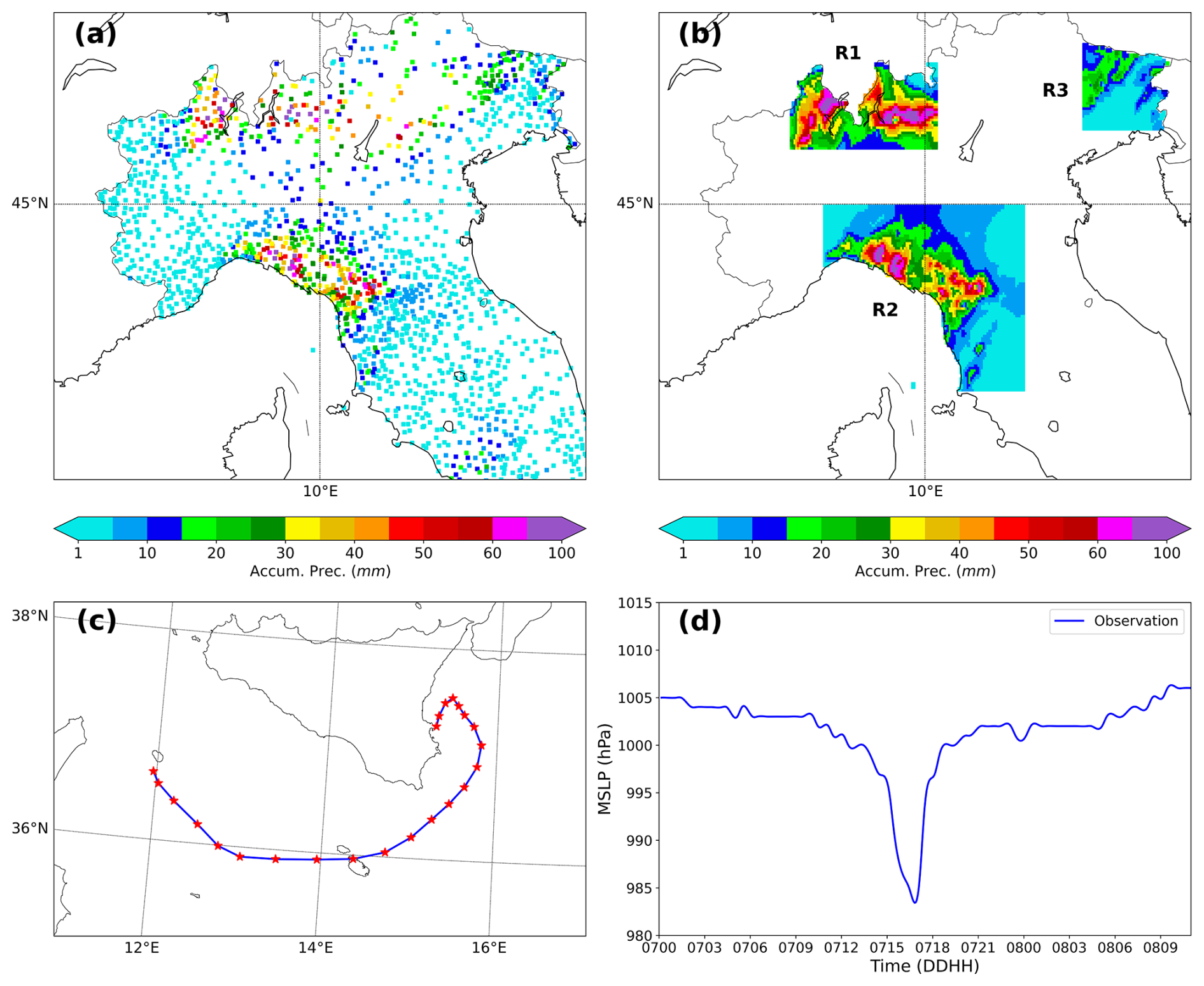
Figure 7 (a) Example of the 12 h accumulated precipitation estimated values and their spatial distribution from the Italian Department of Civil Protection rain gauges. (b) Linear interpolation of 12 h accumulated precipitation values into the three target areas where verification has been performed. (c) Observed track of Medicane Qendresa viewed from infrared satellite imagery. (d) Surface pressure (hPa) data obtained from the METAR station at Malta's airport.

To quantitatively assess the short-term (i.e., first 6–9 h) precipitation forecast for IOP13 initialized using the analysis from the 3D-Var and EnKF DA techniques, a filtering method, relative operating characteristics (ROCs; Mason, 1982; Stanski et al., 1989; Swets, 1973), and Taylor diagrams (Taylor, 2001) were used. We avoid using the conventional point-by-point approach, which has been shown to have serious limitations in the evaluation of high-grid-resolution spatial and temporal precipitation fields (Roberts, 2003). More specifically, we use the fraction skill score (FSS; Roberts and Lean, 2008) as a filtering method, which is commonly used to quantitatively assess precipitation. A preliminary interpolation of the forecast and the observations onto a common regular mesh of 3 km is performed to compute the FSS. The comparison is then carried out within a region of 3×3 grid cells around each grid cell. The FSS can be used to determine the scale over which a forecast system has sufficient skill (Mittermaier and Roberts, 2010). The FSS ranges from 0 to 1, with 1 being a perfect match between the model and the observations. In addition to the receiver operating characteristic (ROC) curves, the area under the ROC curve (AUC; Stanski et al., 1989; Schwartz et al., 2010), which is also widely used to quantitatively assess the quality of weather forecasts, is also used in this study. For a perfect forecast, AUC is equal to 1.

For Qendresa, whisker diagrams (Tukey, 1977) and the probability distribution of cyclone center occurrence (PCCO), which is based on kernel density estimation (KDE; Bowman and Azzalini, 1997; Scott, 2015; Silverman, 2018), were used to validate the simulations. More specifically, the KDE is used to compute the probability of having the center of the cyclone over the entire numerical domain. The main idea behind KDE is to place a “kernel” (i.e., a probability distribution function) at each data point and then sum up the kernels to estimate the overall probability density function. The kernel is typically chosen to be a smooth function, such as a Gaussian function, which decays to zero as the distance from the data point increases. The width of the kernel is controlled by a parameter called the bandwidth, which, as it turns out, is one of the limitations of the KDE technique. In this case, we found that the optimal bandwidth is 20 km, which is within the meso-β scale, i.e., a typical length scale for convective cells. Here, a 2D KDE is applied over each cyclone center (lat–long coordinates) identified for the different simulations (i.e., EnKF vs. 3D-Var). In this way, we infer the most probable track of Qendresa for the different simulations, thereby identifying which is the best DA technique and the one that provides better estimations of Medicane Qendresa's track.

8 Results

As discussed in the previous section, the above-mentioned verification techniques were applied to the two extreme events. The results are described in the following subsections.

8.1 Statistical analysis: IOP13 episode

Because IOP13 was a heavy-rainfall episode, the accumulated precipitation field is used to quantitatively assess the impact of assimilating both in situ conventional and reflectivity observations from Doppler weather radars on short-range forecasts, using the 3D-Var and EnKF DA algorithms.

8.1.1 Filtering method

The FSS associated with the 3 h accumulated precipitation field is computed independently for the three sub-regions, R1, R2, and R3, which are highlighted in Fig. 7b. These regions were chosen due to their higher observation density, allowing for a more reliable evaluation. The analysis is carried out using two precipitation thresholds: 5 mm h⁻¹ (moderate rainfall) and 10 mm h⁻¹ (heavy rainfall). In general, except for R3, the comparison in terms of the FSS (Fig. 8a–f) shows that at the initial forecast time and during the first 6 h, DA simulations (EnKF and 3D-Var) outperform the NODA simulation (without assimilation). Among the DA simulations, EnKF generally outperforms 3D-Var in R1 and R2, especially for the higher-precipitation threshold (10 mm h⁻¹). As expected, CNTRL experiments for both 3D-Var and EnKF provide higher FSS values compared to SYN experiments, where reflectivity observations were not considered.

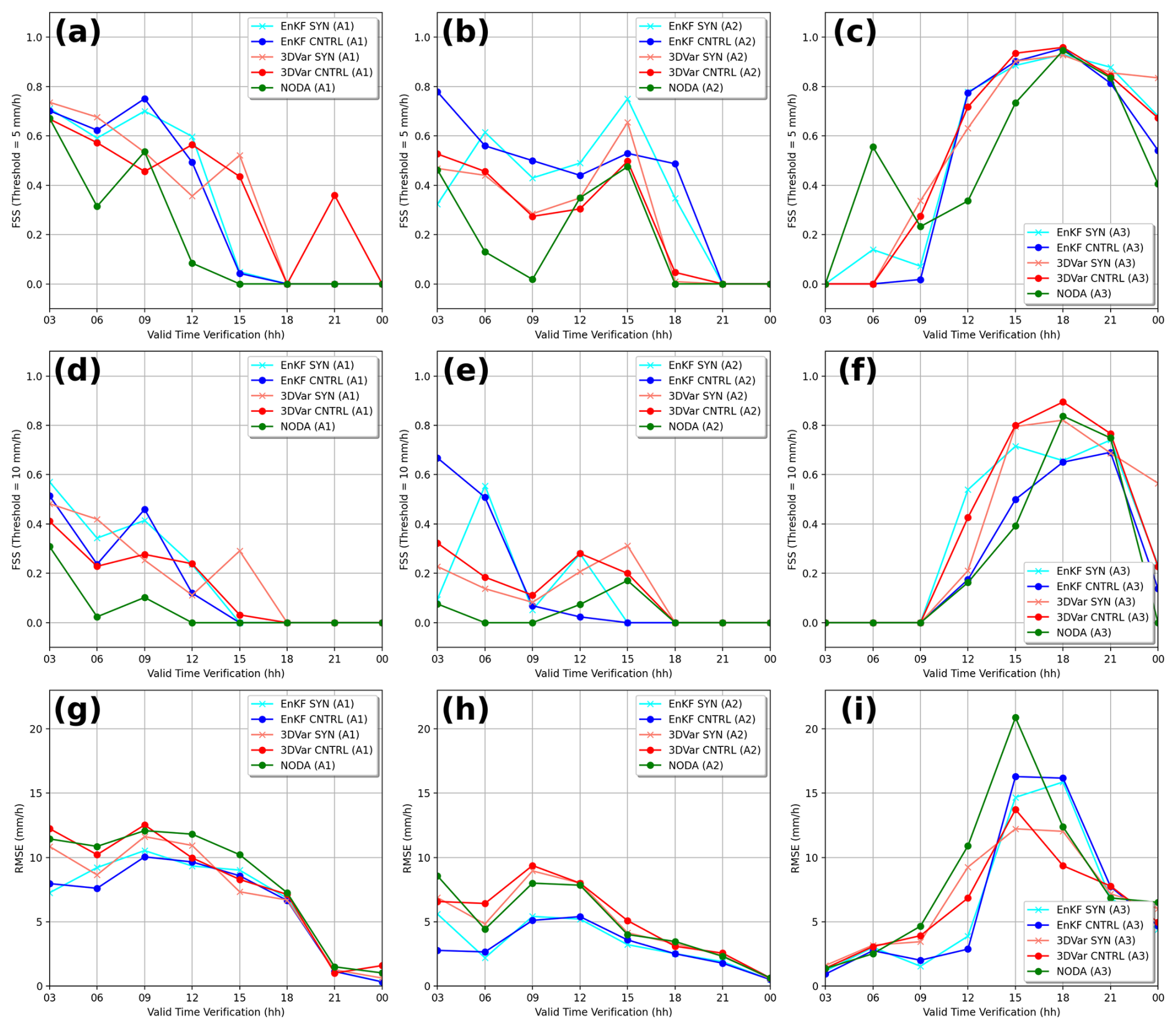
Figure 8 (a–f) Evolution of the FSS during the first 24 h of free forecasts for 3 h accumulated precipitation in the Italian sub-regions: R1 (a, g, d), R2 (b, e, h), and R3 (c, f, i). Two thresholds are used: > 5 mm h⁻¹ (first row) and > 10 mm h⁻¹ (second row). (g–i) Evolution of the RMSE associated with each experiment during the first 24 h of free forecasts in the different sub-regions. Simulations assimilating both conventional and radar observations (CNTRL) and simulations assimilating only conventional observations (SYN) associated with 3D-Var and EnKF are shown here. As a reference, NODA results are also included.

In R3, the results show unexpected behavior when using the moderate threshold (5 mm h⁻¹) (Fig. 8c), where NODA outperforms DA simulations during the first few hours. This anomaly could be attributed to three factors: (1) the use of a moderate-precipitation threshold, which may not capture significant precipitation differences; (2) minimal precipitation in R3 during the initial forecast hours, since the deep convection system had not yet reached this region; and (3) the location of R3 near the domain edges, where it relies solely on in situ observations for assimilation corrections, as it falls outside the radar coverage area. This interpretation is reinforced when examining the higher-precipitation threshold (10 mm h⁻¹) (Fig. 8f), where all methods exhibit similarly poor skill in the early forecast hours, indicating that precipitation is still too weak to be meaningfully assessed. However, after 6–9 h, as expected, DA simulations outperform NODA in all sub-regions.

It should be noted that the CNTRL simulations do not consistently show better FSSs than SYN simulations during the first hours for R1. This could be due to the short-lived impact of radar reflectivity assimilation, which in past studies has been shown to last no longer than 2–4 h for 3D-Var and EnKF. These findings align with those of previous studies, which reported similar behavior regarding the transient impact of reflectivity DA (Carrió and Homar, 2016; Carrió et al., 2019).

Finally, we also computed the root mean squared error (RMSE) for the precipitation field over the first 24 h of the free forecast for both DA and NODA experiments (Fig. 8g–i). For 3D-Var and NODA, RMSE is calculated from the deterministic forecast, while for EnKF, it is computed from the ensemble mean precipitation field. Overall, DA experiments exhibit lower (better) RMSE scores compared to NODA, confirming the positive impact of data assimilation on forecast accuracy. Among the DA experiments, EnKF consistently outperforms 3D-Var in all regions, suggesting a better representation of precipitation variability and improved initial conditions.

8.1.2 ROC and AUC

To strengthen the skill of the different simulations performed by 3D-Var and EnKF, the receiver operating characteristic (ROC) curve is used. The probability of exceeding a given threshold is computed and verified against dichotomous observations. The ROC curve is computed as follows: the model variable is interpolated to the observation locations, and if the model variable exceeds a given threshold, that model grid point is assigned a value of 1. In contrast, if the model value does not exceed that threshold, the assigned value is 0. The same method is applied to the observations. Then, using these dichotomous values, the hit rate and false alarm scores are computed. This process is repeated, varying the threshold value. Gathering the hit rate and false alarm scores for the different thresholds, we obtain the ROC curve. For 3D-Var, we obtain the hit rate and false alarm scores by simply interpolating the model values to the observation locations and apply the threshold criteria explained above. In the case of EnKF, the ensemble mean is used as the field to be interpolated to the observation locations. The area under the ROC curve (AUC), which measures the ability of the system to discriminate between the occurrence or nonoccurrence of the event, is also computed.

For the sake of brevity and because the results from the three sub-regions are similar, the ROC curve and AUC are computed, accounting for all the observations within the inner domain. Specifically, to compute the ROC curves, we use the 3 h (from 00:00–03:00 UTC on 15 October) and 6 h (from 00:00–06:00 UTC on 15 October) accumulated precipitation fields from the model simulation and the observed values registered by the rain gauges, using 1 and 10 mm as thresholds (Fig. 9).

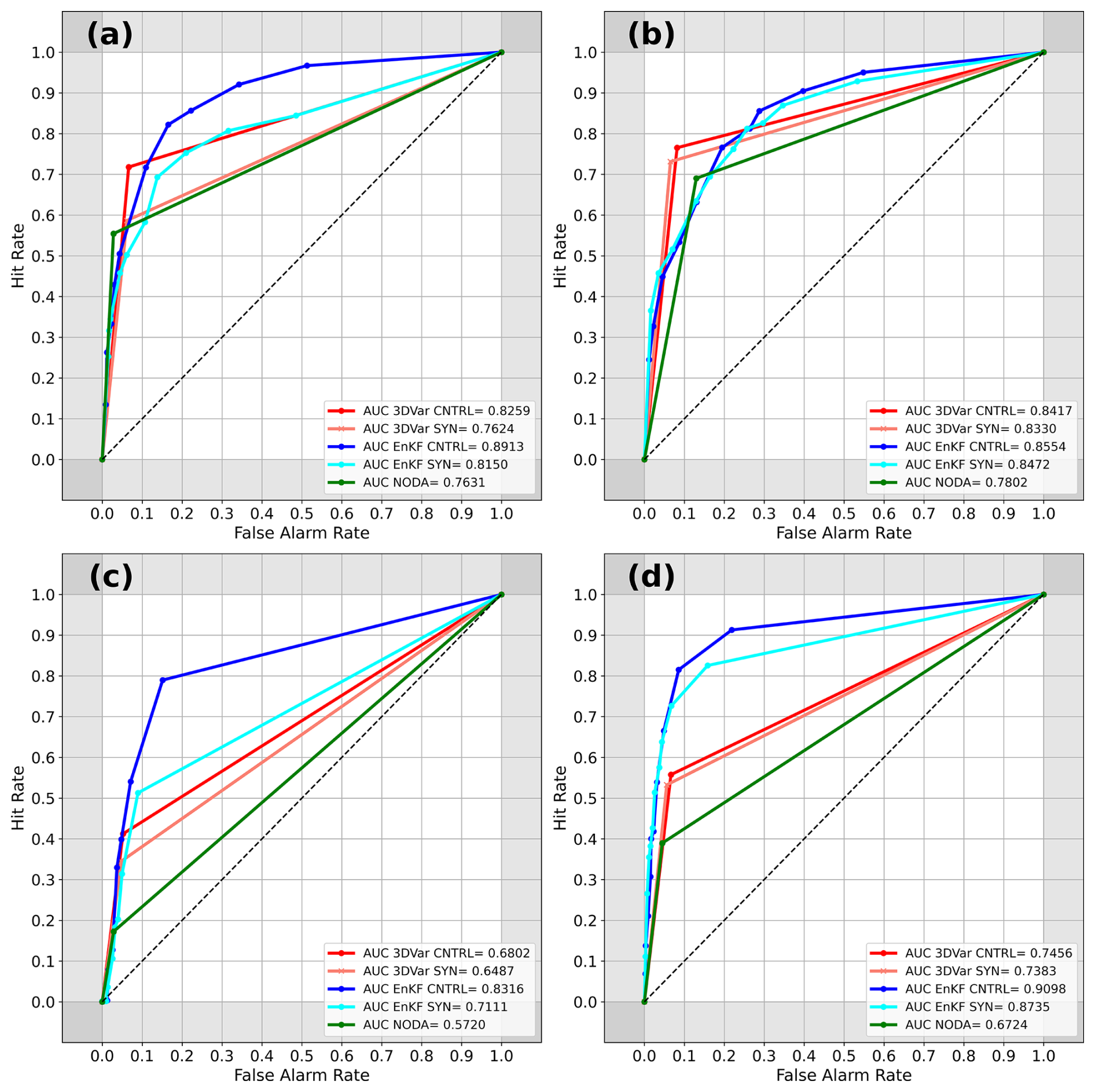
Figure 9 ROC curves and AUC associated with 3D-Var (red and pink colors), EnKF (blue and cyan colors), and NODA (green color) for the 3 h accumulated precipitation using (a) 1 mm and (b) 10 mm thresholds and 6 h accumulated precipitation using (c) 1 mm and (d) 10 mm thresholds, computed over the entire inner domain. Note: all experiments employ the same set of probability thresholds; any apparent differences in the number of plotted points arise from the clustering of ROC values at similar thresholds, not from differing data counts.

Overall, DA experiments outperform the NODA runs for both the 3 h and the 6 h accumulated precipitations, as shown by higher ROC curves and larger AUC values. Among the DA approaches, EnKF consistently outperforms 3D-Var, with greater benefits observed at the 10 mm threshold (i.e., bottom row of Fig. 9). This improvement highlights the advantages of radar reflectivity assimilation within an ensemble-based framework, especially for more intense precipitation events. To better understand this result, we closely analyzed the 1 and 6 h accumulated precipitation fields obtained from EnKF (CNTRL) and 3D-Var (CNTRL), comparing them against corresponding observations (see Figs. A1 and A2 in Appendix A). The 1 h accumulated precipitation (Fig. A1) shows that EnKF localizes the regions where the most intense precipitation was observed with high accuracy, that is, near Tuscany and northern Italy. Moreover, 3D-Var correctly reproduces rainfall in the regions affected by observed precipitation, although the maximum amounts are centered over Liguria instead of near Tuscany. In addition, 3D-Var also shows a tongue area of weak precipitation from Liguria to northern Italy, which does not fit with the observations. Consequently, while small differences exist between 3D-Var and EnKF in the 1 h accumulated precipitation field, the low magnitude of accumulated precipitation values leads to no substantial differences in ROC verification scores. However, in the case of the 6 h accumulated precipitation (Fig. A2), 3D-Var overestimates accumulated precipitation near Liguria, Tuscany, and northern Italy compared to the observations. Moreover, 3D-Var also misplaces the locations of the precipitation for some places. In contrast, EnKF locates the regions where the accumulated precipitation was actually observed with enough accuracy and properly estimates the observed intensity. Consequently, the ROC curve for the 6 h accumulated precipitation obtained from EnKF produced a much better score than 3D-Var. We hypothesize that this difference could be associated with the static/climatological background error covariance matrix used by 3D-Var. Because of the fast changes in the flow associated with the IOP13 case, using a climatological background error covariance would not be as good as using a flow-dependent background error covariance matrix, which is used in EnKF.

8.1.3 Taylor diagrams

To strengthen the comparison of the DA schemes, a Taylor diagram is used. This tool provides us with additional information about the skill of each ensemble member in EnKF. Here, we compute the Taylor diagram for the 6 and 24 h accumulated precipitation fields, which represent the forecast ranges where the assimilated observations have more impact. Overall, results show that the NODA experiment generally exhibits the lowest correlation and largest discrepancy in standard deviation relative to observations, emphasizing that DA significantly improves the representation of precipitation fields, especially for high-impact weather events. Among the different DA approaches, the 3D-Var and the EnKF ensemble mean provide comparable results, with correlations ranging from approximately 0.50 to 0.61, and a similar RMSE and standard deviation that are symmetrically distributed around the observed reference. Notably, 3D-Var tends to overestimate the standard deviation, while the EnKF ensemble mean tends to underestimate it (Fig. 10). A key advantage of EnKF lies in its individual ensemble members, some of which exhibit better performance than the 3D-Var run. Although the mean difference between EnKF and 3D-Var is small, the ensemble-based approach provides additional insight through its member-by-member variability. Specifically, ensemble members using the Grell–Freitas cumulus parameterization coupled with the Yonsei University planetary boundary layer scheme exhibit higher correlations and standard deviations that are similar to the observations in this study. Conversely, ensemble members associated with lower scores are those using the Kain–Fritsch scheme for the cumulus parameterization and the Mellor–Yamada–Janjić scheme for the planetary boundary layer scheme. These findings underscore the potential of multiphysics ensembles to capture diverse physical representations of convective processes, thereby enhancing forecast accuracy.

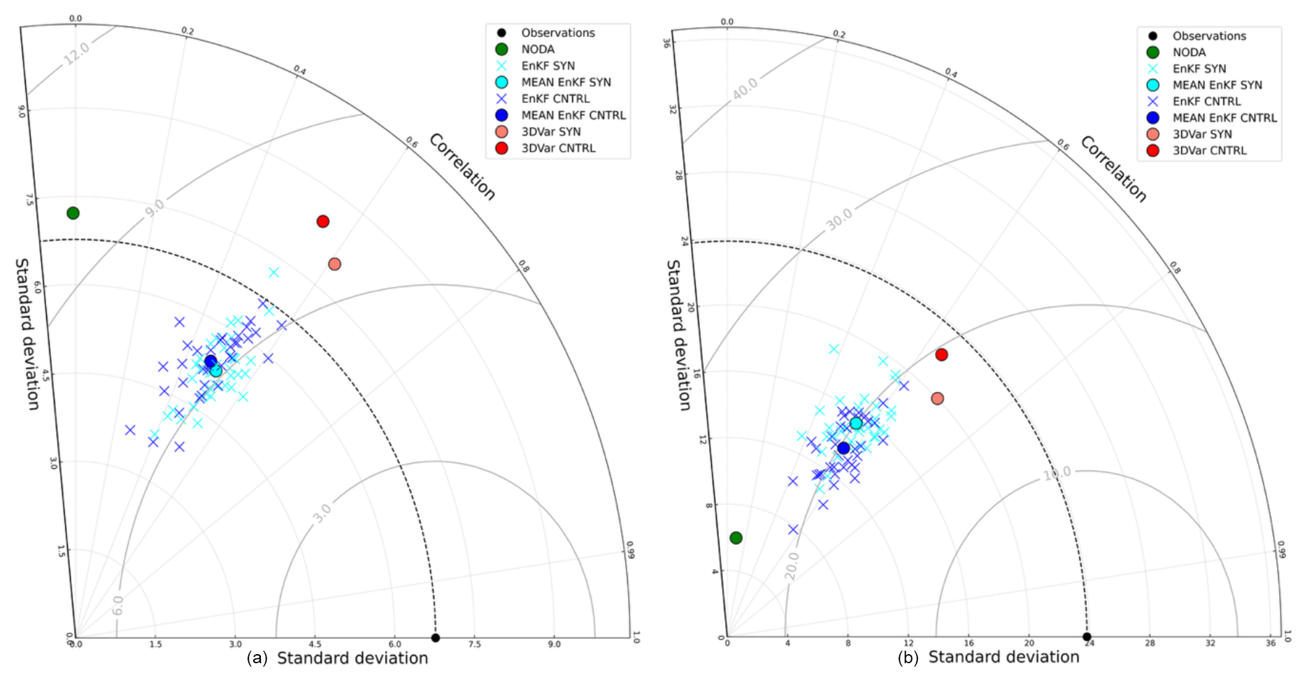
Figure 10 Taylor diagram comparing the performance of 3D-Var (red), EnKF (blue), and NODA (green) for the (a) 6 h and (b) 24 h accumulated precipitation, valid at 06:00 UTC on 15 October 2012.

8.2 Statistical analysis: Qendresa event

In tropical cyclone forecasting, two key factors are typically evaluated: (a) the intensity and (b) the trajectory followed by the cyclone. Therefore, to assess the impact of assimilating both in situ conventional and remote RSAMV observations using 3D-Var and EnKF, we focus on these two factors for the Qendresa event.

8.2.1 Whisker diagrams

For this event, the lack of in situ observations over maritime regions poses the main challenge to properly verifying the triggering and intensification of cyclones. Fortunately, Medicane Qendresa crossed just over Malta, where a pressure drop greater than 20 hPa in 6 h was registered by METAR at Malta's airport, reaching a minimum surface pressure of 985 hPa. Therefore, METAR is used to quantitatively assess the skill of the NODA simulation and the various DA approaches. To compare the surface pressure registered in Malta with the different simulations, the full cyclone trajectory is used, and the grid point closest to Malta's airport is selected. Specifically, the surface pressure time series measured by METAR is compared with the NODA run and the different DA simulations from 3D-Var and EnKF, such as 3D-Var_SYN, 3D-Var_CNTRL, EnKF_SYN, and EnKF_CNTRL (Fig. 11).

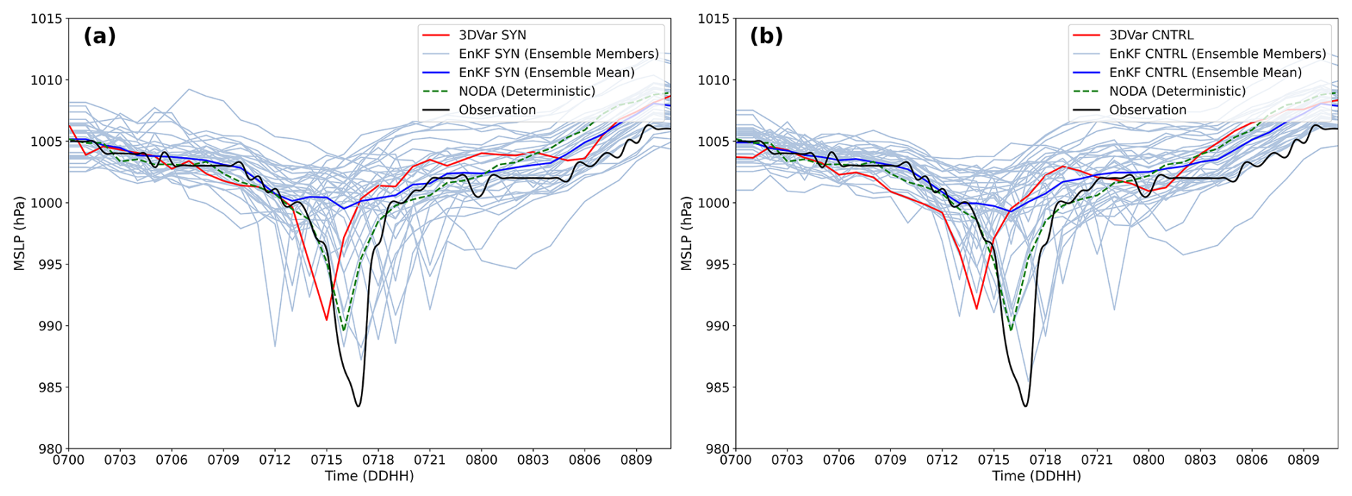
Figure 11 Temporal surface pressure evolution at the closest grid point to Malta for the (a) SYN and (b) CNTRL experiments associated with EnKF (blue), 3D-Var (red), and NODA (green) compared to the observed surface pressure registered by METAR in Malta's airport (black line).

Overall, results indicate that the NODA simulation captures the timing of the observed pressure drop more accurately than the DA runs, suggesting that the large-scale dynamics are adequately represented even without data assimilation (Fig. 11). However, NODA underestimates the intensity of the medicane's central pressure.

Among the DA simulations, assimilating in situ conventional observations enables some EnKF ensemble members to outperform NODA in both timing and intensity, whereas 3D-Var shows limitations in capturing the event timing and central pressure depth (Fig. 11a). Additionally, the ensemble mean of EnKF_SYN accurately fits the observations during the first hours of the forecast, from 00:00 to 13:00 UTC on 7 November (Fig. 11a), performing slightly better than 3D-Var_SYN. However, during the intensification phase, the ensemble mean of EnKF_SYN barely shows the intensification of Qendresa, reaching minimum MSLP values of 1002 hPa. In contrast, the 3D-Var_SYN simulation depicts the intensification of the medicane by deepening the MSLP and reaching values of 992 hPa, although a time shift of 3 h is found (i.e., 15:00 UTC on 7 November) (Fig. 11a). Finally, during the dissipation phase of Qendresa, the ensemble mean of EnKF_SYN performs slightly better than that of 3D-Var_SYN (Fig. 11a). These results highlight a notable limitation of EnKF when applied to low-predictability weather events, such as Qendresa. The low predictability of Qendresa and the high sensitivity to physical parameterizations produce substantial spread in ensemble behavior: some members capture the cyclone's closed circulation and track reasonably well, while others fail to develop a coherent low-pressure core, instead producing only disorganized or weak convective cells. Consequently, these poorly performing members may entirely miss the medicane's formation or misplace its center, leading to large errors in both track and intensity forecasts. In this situation, our small to moderate ensemble size exacerbates sampling error, yielding spurious background error covariances that degrade analysis accuracy in EnKF. These errors become particularly problematic when the numerical model mispredicts the event, since the ensemble members no longer provide a reliable representation of flow-dependent uncertainty. On the other hand, a climatological/static background error covariance matrix, like the one used in 3D-Var, could produce better results than ensemble members, as we see in Fig. 11a, where we compare 3D-Var (red line) with the EnKF ensemble mean analysis (blue line). Moreover, it is important to note that although the ensemble mean of EnKF_SYN does not correctly reproduce the intensification of Qendresa, some of the ensemble members reproduce the observed MSLP very well, in both deepening and timing. This suggests that using an ensemble system, even when having the above-mentioned problems, is still more useful than using only a fully deterministic system such as 3D-Var, which cannot provide information about the uncertainties of the system. Therefore, we can speculate that for extreme weather events with low numerical predictability, a better approach could be using a hybrid error covariance model, where the forecast error covariance matrix is obtained linearly by combining ensemble-based covariance with static climatological error covariances (Hamill and Snyder, 2000; Lorenc, 2003; Clayton et al., 2013; Carrió et al., 2021). The impact of using hybrid DA to improve these kinds of small-scale extreme weather events could be of great interest in the weather forecast community, although it is beyond the scope of this study. For this reason, the authors leave the benefits of using hybrid error covariance models to improve the forecast of extreme weather events in the Mediterranean Basin for future work.

We then evaluated the impact of assimilating both in situ conventional and RSAMV observations on the accuracy of the Qendresa intensity forecast (Fig. 11b). In this case, the results of the two experiments show large similarities (Fig. 11a, b). In terms of 3D-Var, the MSLP signature is basically the same, without showing a clear signal of improvement or diminishing, suggesting that the assimilation of RSAMVs is not enough to significantly improve the relevant low-level dynamical structures associated with the genesis and intensification of Qendresa. However, in terms of EnKF, a clear improvement is found for a few members, even if it does not affect the mean value. Indeed, some of the ensemble members that depicted an intense cyclone far from the time when it was observed (at approx. 18:00 UTC on 7 November) were corrected, reducing spurious cyclones and bringing at least one ensemble member closer to the observed value (Fig. 11b). It can be observed that in EnKF_CNTRL, there are more ensemble members depicting a deep cyclone at the observed time than in the case of EnKF_SYN, showing the benefits of assimilating RSAMVs to improve the intensification estimation of Qendresa.

To quantitatively assess the performance of NODA and the different DA experiments, we use the lagged-correlation technique computed between the model MSLP signatures and the observations. This technique allows us to measure how the shape of the surface pressure evolution obtained from the different simulations fits the shape of the observed MSLP, also taking temporal shifting into account. The correlation is computed for NODA, 3D-Var, and each ensemble member from EnKF. These results are shown using whisker plots (Fig. 12), where a correlation of 1 indicates that the specific model field has the same “V” pressure shape evolution as the observation and that the minimum for both is found at the same time. The results show that the NODA simulation exhibits the highest correlation values among all the simulations, reaching its maximum correlation when no time shifting is applied. For 3D-Var_SYN, the correlation is at its maximum and approximately equal to 1 when a 1 h delay is produced by the forecasts (Fig. 12a). Whiskers from EnKF_SYN show that none of the ensemble members overcomes the maximum correlation value found in 3D-Var_SYN. However, when the assimilation of RSAMVs is added to the in situ conventional observations, it is found that the maximum correlation value associated with 3D-Var_CNTRL using 2 h of delay applied to the forecasts is surpassed by some of the ensemble members of EnKF_CNTRL, when a 3 or 4 h delay is applied (Fig. 12b).

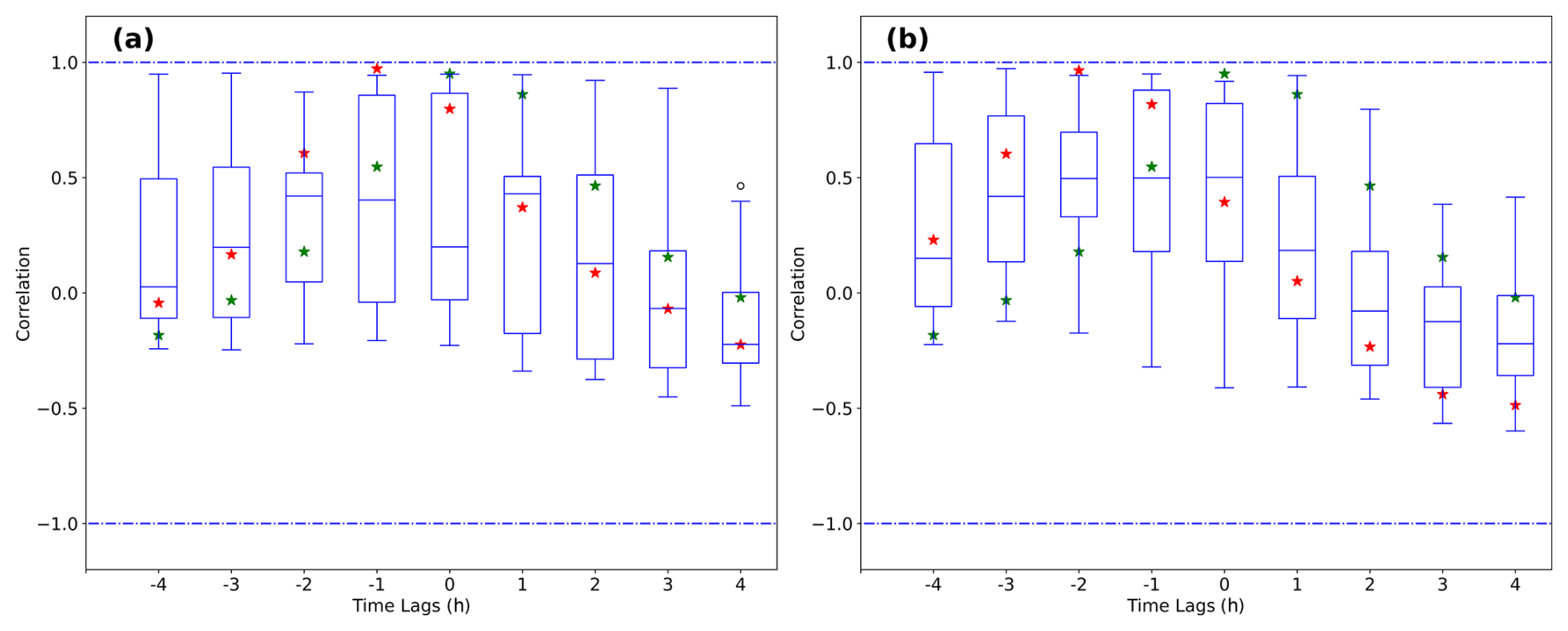
Figure 12 Whisker plots depict the lagged-correlation values between the observations and EnKF (blue boxes), 3D-Var (red stars), and NODA (green stars) for the (a) SYN and (b) CNTRL experiments. The correlation is computed considering that the observed V-shape pressure signature associated with the observations is shifted 4 h to the left and 4 h to the right.

8.2.2 Probability distribution of cyclone center occurrence

Due to the difficulty of accurately predicting the observed trajectory of Qendresa (Pytharoulis, 2018), the impact of assimilating different kinds of observations on the trajectory of the medicane is investigated.

Results indicate that the NODA simulation fails to accurately capture the track of Qendresa, especially its recurvature towards Sicily after leaving Malta, as evidenced by satellite imagery. In contrast, 3D-Var_SYN accurately captures the track of Qendresa during the first hours (Fig. 13b). However, after Qendresa leaves Malta, the trajectory simulated by 3D-Var_SYN diverges from the observed track, shifting northeastwards and failing to capture the track loop observed in satellite imagery. To quantify the benefits of assimilating in situ conventional observations using 3D-Var or EnKF, the probability of occurrence of a cyclone following the track observed via satellite imagery is computed. For instance, 3D-Var_SYN underestimates the probability of cyclone occurrence east of Sicily, where Qendresa made landfall while looping (Fig. 13b). On the other hand, some EnKF_SYN ensemble members show a cyclone trajectory shifted significantly southward, while others reproduce the loop trajectory missed by the NODA forecast (Fig. 13a). In addition, the probability of Qendresa occurring eastwards of Sicily is in this case larger than that of 3D-Var_SYN, showing the benefits of using EnKF against 3D-Var (Fig. 13a). Moreover, the EnKF_SYN ensemble trajectories generally follow a V shape (i.e., first moving towards the southeast, then moving to the east, and finally moving towards the northeast), similar to the trajectory observed via satellite imagery. Although the shapes of most of the EnKF_SYN trajectories agree with the observations, a consistent southeastward displacement is evident in their location.

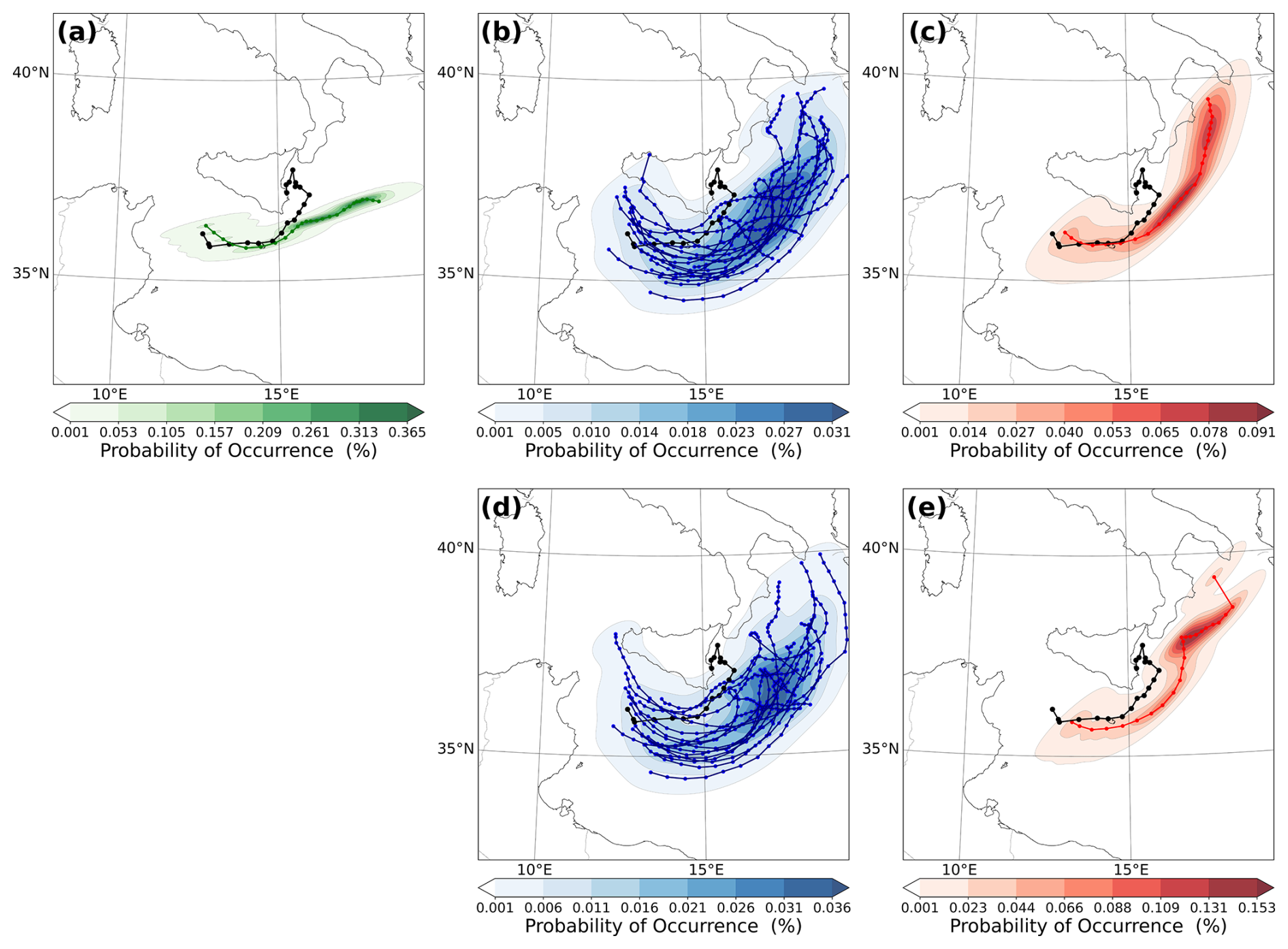
Figure 13 Probability of cyclone center occurrence (within 20 km) computed using Gaussian KDE for (a) NODA, (b) EnKF (SYN), (c) 3D-Var (SYN), (d) EnKF (CNTRL), and (e) 3D-Var (CNTRL), from 11:00 UTC on 7 November to 12:00 UTC on 8 November 2014. Qendresa's trajectory observed via satellite imagery is depicted in black.

If both in situ conventional and RSAMV observations are assimilated, some of the ensemble members from EnKF_CNTRL show more accurate trajectories in comparison with EnKF_SYN: the loop trajectory is closer to the observed region of eastern Sicily (Fig. 13c). An improvement of the 3D-Var_CNTRL trajectory by increasing the probability of cyclone occurrence following the observed track is observed, especially in eastern Sicily. However, 3D-Var experiments are not able to reproduce the looping trajectory observed via satellite imagery (Fig. 13b–d). Hence, EnKF outperforms 3D-Var, with some ensemble members depicting a loop trajectory, although shifted southwards, and producing a probability of cyclone occurrence lower than 3D-Var.

Both EnKF and 3D-Var still have difficulties in accurately depicting the track observed by Qendresa, even after the assimilation of in situ conventional and RSAMV observations. Because RSAMVs are useful for describing dynamical features in the upper levels of the atmosphere, we hypothesize that incorporating them via DA may not be sufficient to correct key low-level dynamical features. In this case, the assimilation of surface wind observations may even help to improve these results. However, this is beyond the scope of this study, and the authors leave this question for future work, where other sources of information from satellites will be assimilated to improve the low-level thermodynamic aspects of extreme weather events, such as medicanes.

9 Summary and conclusions

This study provides a quantitative assessment of the impact of two widely used DA techniques – 3D-Var and EnKF – on the predictability of maritime extreme weather events. The focus is on evaluating their potential to improve forecast lead time by assimilating observations during the developing stage, as opposed to the mature stage, which affords limited time for preparedness and response. To evaluate the performance of 3D-Var and EnKF, we analyze two high-impact weather events that were triggered over the sea and later affected densely populated coastal regions. These two extreme weather events are known as (a) the high-precipitation event registered during the 13th intensive observation period (IOP13) affecting the western, northern, and central parts of Italy, and (b) the intense tropical-like Mediterranean cyclone (medicane) known as Qendresa, which affected the islands of Pantelleria, Lampedusa, Malta, and Sicily. These weather events pose a serious challenge for the numerical weather prediction community due to their low predictability, resulting from their initialization over the sea, where in situ observations are sparse and initial conditions are poorly estimated. Furthermore, their evolution over complex-terrain regions introduces additional forecasting challenges.

For these two extreme weather events, both 3D-Var and EnKF DA methods were applied, with the type and number of assimilated observations varying based on the data availability. For Qendresa, we assimilated (a) hourly in situ conventional observations and (b) wind speed and wind direction profiles of the entire atmosphere (RSAMVs) derived from geostationary satellites every 20 min, providing high-spatial- and high-temporal-resolution observations covering the central Mediterranean Sea, where Qendresa was initiated and evolved. On the other hand, for the IOP13, we assimilated (a) hourly in situ conventional observations and (b) 15 min 3D reflectivity observations from two type-C Doppler weather radars.

Because of the different thermodynamic characteristics associated with Qendresa and IOP13, a set of different verification metrics was used for each of these extreme weather events. A filtering method (FSS and RMSE), ROC/AUC, and Taylor diagram were used to verify the numerical simulations from 3D-Var and EnKF associated with IOP13. In the case of Qendresa, we used whisker diagrams and the probability distribution of cyclone center occurrence verification scores. For the IOP13, both the filtering method and the Taylor diagram verification show that EnKF slightly outperforms 3D-Var, although the differences are not significant. In addition, it was observed that the assimilation of spatial and temporal high-resolution reflectivity observations significantly improved the forecast for both 3D-Var and EnKF, showing the key role of this type of observation. On the other hand, the ROC and AUC scores clearly show that EnKF outperforms 3D-Var. For the Qendresa event, while the ensemble mean of EnKF underestimates the intensity of the medicane compared to 3D-Var, some individual EnKF ensemble members produce more accurate results than 3D-Var. This behavior suggests how important it is to use an ensemble forecast system to predict extreme weather events at high spatial and temporal resolutions. Regarding the cyclone's trajectory, EnKF provides a more realistic representation of Qendresa's observed path.

Although the EnKF technique has generally shown better performance against 3D-Var for the two extreme weather events analyzed in this study, it is also important to account for the computational resources required by each method. EnKF requires approximately 36 times more model integrations per cycle than 3D-Var's single forecast, in addition to the overhead of computing ensemble updates. This makes 3D-Var appealing because it is much faster and cheaper than EnKF, and it makes this technique particularly suitable for operational purposes at small weather forecast centers.

An interesting result of this study is that, for highly non-Gaussian extreme events, the deterministic 3D-Var forecast can occasionally outperform the EnKF ensemble mean in terms of point forecasts (e.g., minimum central pressure) because averaging across ensemble members tends to smooth out the tails of a skewed probability distribution. In contrast, probabilistic metrics like ROC/AUC consistently favor EnKF, reflecting its superior ability to capture forecast uncertainty. We attribute these contrasting behaviors to the different approaches to background error covariances: 3D-Var employs a static covariance, while EnKF uses a flow-dependent covariance estimated from a finite ensemble. To combine the strengths of both methods, a hybrid error covariance approach – where the forecast error covariance matrix is formed by linearly blending the EnKF's ensemble-derived covariances with the 3D-Var's static climatological covariances – may offer improved forecast skill for convective-scale extreme events.

Further work will investigate the impact of using hybrid DA schemes in comparison to standard 3D-Var or EnKF. In this scenario, it is expected that the hybrid error covariance matrix will be more precise than the one derived from the ensemble members or from climatology, which on their own are not able to reproduce key aspects of challenging extreme weather events. High temporal and spatial observations from Doppler weather radars, such as reflectivity and radial wind velocities, will be assimilated for this case to obtain accurate analysis and, thus, improve the short-range forecast of this catastrophic flash flood event. In addition, it is important to highlight that satellite-based data assimilation provides a significant opportunity for enhancing convective-scale forecasting, particularly in data-sparse maritime regions such as the Mediterranean, where the formation of extreme weather events like tropical-like cyclones increasingly impacts densely populated areas. Future studies integrating high-resolution satellite observations, such as cloud top heights, thermodynamic profiles, or cloud properties, could further enhance the accuracy of convective-scale predictions, improving early warning capabilities and disaster preparedness.

Appendix A

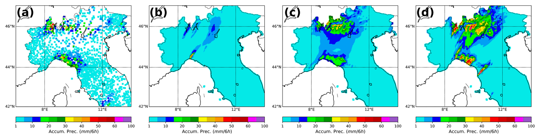
Figure A1 The 1 h accumulated precipitation computed from 00:00–06:00 UTC on 15 October 2012 associated with observations (first column), NODA (second column), EnKF (CNTRL) (third column), and 3D-Var (CNTRL) (fourth column).

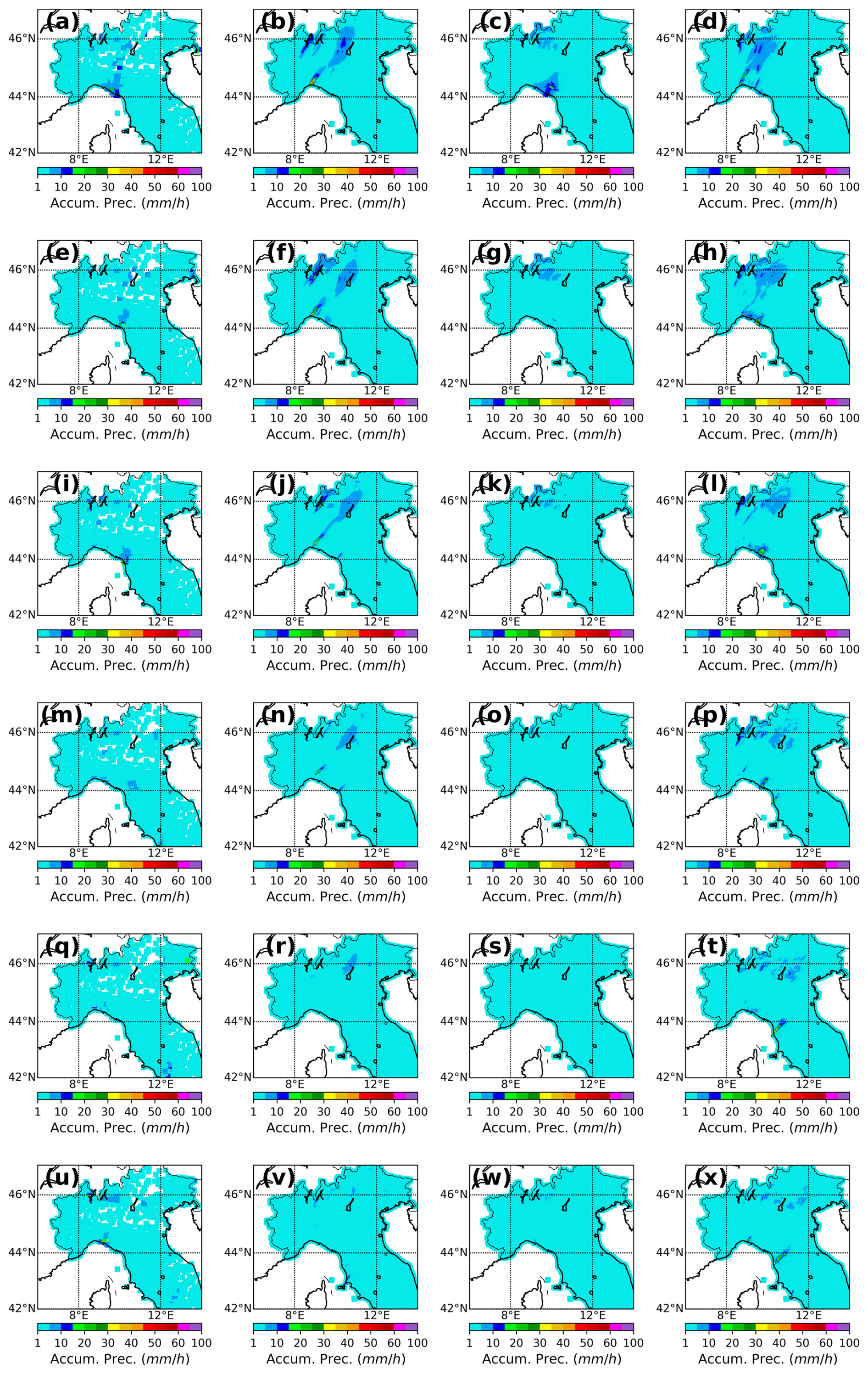
Figure A2 The 6 h accumulated precipitation computed from 00:00–06:00 UTC on 15 October 2012 associated with (a) observations, (b) NODA, (c) EnKF (CNTRL), and (d) 3D-Var (CNTRL).