Investigation of an extreme rainfall event during 8–12 December 2018 over central Vietnam – Part 2: An evaluation of predictability using a time-lagged cloud-resolving ensemble system​​​​​​​

This is the second part of a two-part study that investigates an extreme rainfall event that occurred from 8 to 12 December 2018 over central Vietnam (referred to as the D18 event). In this part, the study aims to evaluate the practical predictability of the D18 event using the quantitative precipitation forecasts (QPFs) from a time-lagged cloud-resolving ensemble system. To do this, 29 time-lagged (8 d in forecast range) high-resolution (2.5 km) members were run, with the first member initialized at 12:00 UTC on 3 December and the last one at 12:00 UTC on 10 December 2018. Between the first and the last members are multiple members that were executed every 6 h. The evaluation results reveal that the cloud-resolving model (CReSS) predicted the rainfall fields in the short range (less than 3 d) well for 10 December (the rainiest day). Particularly, the CReSS model shows high skill in heavy-rainfall QPFs for this date with a similarity skill score (SSS) greater than 0.5 for both the last five members and the last nine members. The good results are due to the model having good predictions of relevant meteorological variables such as surface winds. However, the predictive skill is reduced at lead times longer than 3 d, and it is challenging to achieve good QPFs for rainfall thresholds greater than 100 mm at lead times longer than 6 d. These results also confirmed our scientific hypothesis that the cloud-resolving time-lagged ensemble system (using the CReSS model) improved the QPFs of this event in the short range. Furthermore, the results also demonstrated that a decent QPF can be made at a longer lead time (by a member initialized at 18:00 UTC on 4 December).

In addition, the ensemble-based sensitivity analysis (ESA) of 24 h rainfall in central Vietnam shows that it is highly sensitive to initial conditions, not only at lower levels but also at upper levels. The rainfall is sensitive to both kinematics and moisture convergence at low levels, and such sensitivities decrease with increasing lead time. The ESA also facilitates a better understanding of the mechanisms in the D18 event, implying that it is meaningful to apply ESA to control initial conditions in the future.

1 Introduction

The present study is the second part of a two-part study investigating the extreme rainfall event during 8–12 December 2018 over central Vietnam (referred to as the D18 event hereafter). In this event, record-breaking rainfall occurred along the mid-central coast of Vietnam, from Quang Binh to Quang Ngai provinces. The observation shows that the peak amount in rainfall accumulation in particular exceeded 800 mm over a 3 d period from 12:00 UTC on 8 December to 12:00 UTC on 11 December (Fig. 1f). During this period, the rainiest day was 10 December, with the 24 h observed amount exceeding 600 mm at some stations (Fig. 4 “OBS”). This record-breaking rainfall event led to 13 deaths, widespread destructions in the environment and downstream cities, and heavy economic losses due to catastrophic flooding and landslides (Tuoi Tre news, 2018). In Part 1 (Wang and Nguyen, 2023), we focused on the analysis of the mechanism that caused this event and evaluated the simulation using the Cloud-Resolving Storm Simulator (CReSS; Tsuboki and Sakakibara, 2002, 2007). The analysis results point out the main factors which led to this event as well as its spatial rainfall distribution. These factors included the combined interaction between the strong northeasterly winds and easterly winds over the South China Sea (SCS) in the lower troposphere (below 700 hPa). The local terrain also played an essential role due to its barrier effect. The cloud model's good simulation results in Part 1 indicated its promising potential in forecasting this event. Hence, in Part 2, the present study focuses on an evaluation of its predictability of the D18 event through a series of time-lagged high-resolution ensemble quantitative precipitation forecasts (QPFs) by the CReSS model.

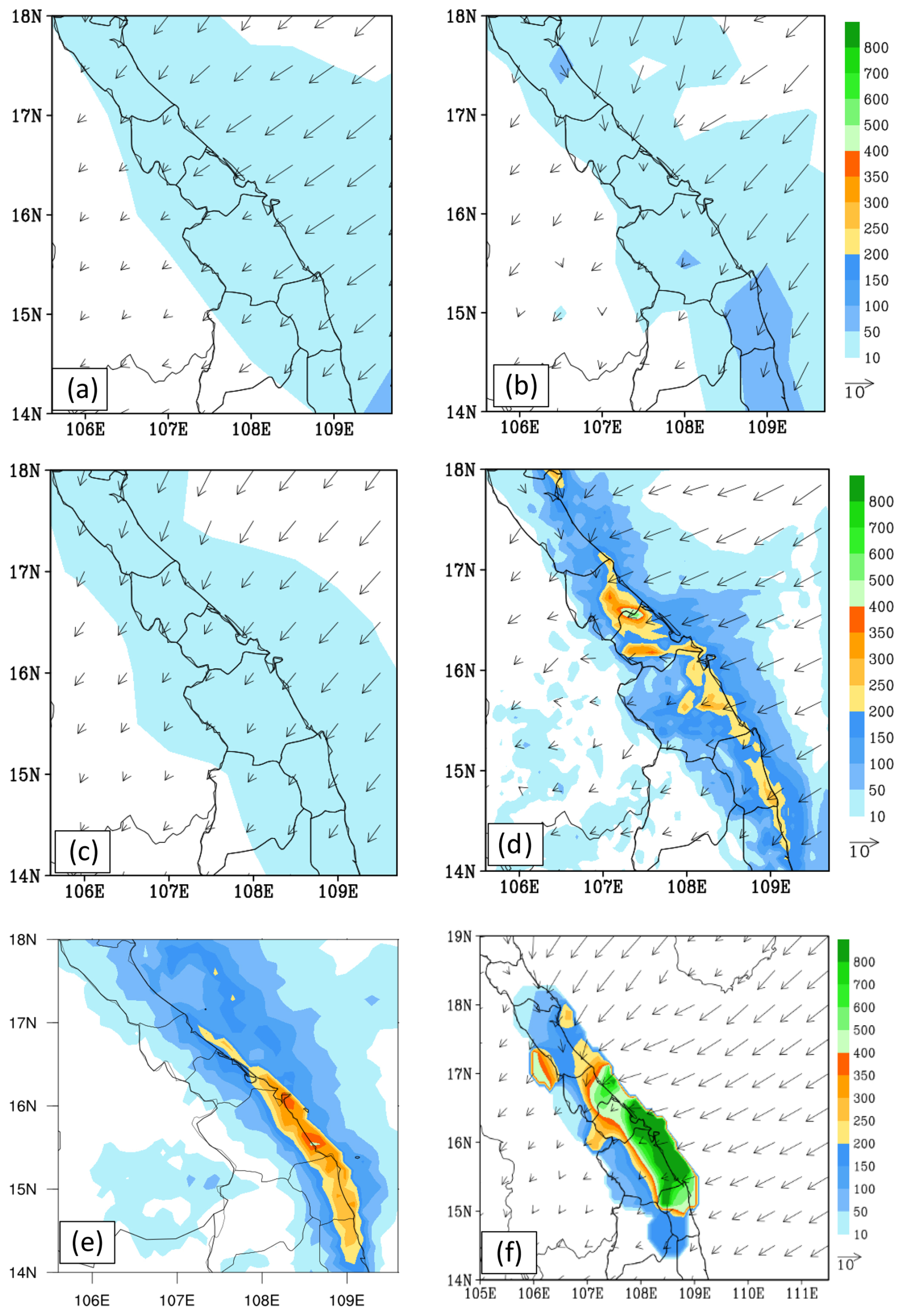
Figure 1 The predicted 72 h accumulated rainfall (mm, shaded) and mean surface wind (m s⁻¹, vector) for the period of 12:00 UTC on 8 December–12:00 UTC on 11 December 2018 obtained by (a) NCEP, (b) ECMWF, (c) JMA, (d) WRF, (e) 72 h accumulated rainfall obtained by the Global Precipitation Measurement (GPM) estimate (IMERG Final Run product), and (f) 72 h in situ-observed accumulated rainfall (mm, shaded) and the mean surface wind derived from ERA5 data (m s⁻¹, vector), adapted from Fig. 14c of Wang and Nguyen (2023).

Predicting heavy-rainfall events is still challenging to meteorologists and weather forecasters, although great progress has been made in the science of numerical weather prediction. The prediction of heavy to extreme rainfall is more difficult for Vietnam, where both multi-scale interactions among different weather systems and strong influences of local topography often exist. For example, when D18 event occurred, several operational models were unable to predict this event successfully. Specifically, Fig. 1 shows the predictions for the D18 event by three global models at the National Centers for Environmental Prediction (NCEP), the European Centre for Medium-Range Weather Forecasts (ECMWF), and the Japan Meteorological Agency (JMA) and by one mesoscale regional model, the Weather Research and Forecasting (WRF) model, implemented for operation at the Mid-Central Regional Hydro Meteorological Center in Da Nang city, Vietnam, with the finest horizontal grid spacing (Δx) of 6 km × 6 km. While these models overall made good predictions in the surface wind field, their 72 h accumulated rainfall amounts along the coast of central Vietnam were less than 250 mm and much lower than the observation, which exceeded 900 mm (Fig. 1). Therefore, in order to improve the QPFs for heavy-rainfall events in Vietnam, we need to not only understand the events' mechanisms of occurrence, but also adopt or develop better forecasting tools, a more effective strategy, or both.

Among several different methods, present-day weather forecasts depend mainly on numerical weather prediction (NWP) using models, a scientific method that simulates weather and produces quantitative results (Fig. 1). However, there is always uncertainty in numerical forecasts due to the fact that the atmosphere is a chaotic system and tiny errors in the initial state can grow rapidly and lead to larger errors in the forecast (Hohenegger and Schär, 2007; Lorenz, 1969a, b). Various approximations in numerical methods are also sources of forecast uncertainty. Thus, by generating a range of possible weather conditions in the days ahead or further into the future, ensemble forecasting was introduced as an effective method to estimate forecast uncertainty and improve the overall accuracy and usefulness of NWP products. This is because the ensemble mean typically has smaller errors than individual members, since the high-predictability features that the members agree on are emphasized by the mean, while the low-predictability ones that the members do not agree on are filtered out or dampened (e.g. Leith, 1974; Murphy, 1988; Surcel et al., 2014). However, this may smooth out extreme events and underestimate their magnitude. Furthermore, some studies have shown high skill in QPFs for extreme rainfall produced by typhoons in Taiwan using the CReSS model, a cloud-resolving model (CRM) with high resolution and a time-lagged approach (Wang et al., 2016; Wang, 2014; Wang et al., 2015, 2013, 2023). Table 1 of Wang et al. (2016) shows that the high-resolution time-lagged ensemble forecasts provide overall better quality in comparison with both the traditional low-resolution ensemble forecasts and high-resolution deterministic forecasts at a comparable cost in computation.

Besides the advantages of ensemble forecasts described above, ensemble-based sensitivity analysis (ESA) also provides an effective method to investigate how sensitive the forecast variables are and to what preceding factors they are sensitive. To be more specific, Torn and Hakim (2009) used ESA to evaluate how their subject, a group of tropical cyclones (TCs) undergoing extratropical transition, in predictions responds to changes in the initial conditions. In their results, the forecasts of cyclone minimum sea-level pressure are determined to be strongly sensitive to TC intensity and position at short lead times and equally sensitive to mid-latitude troughs that interact with the TC at longer lead times. For an extreme rainfall event in northern Taiwan, Wang et al. (2021) performed ESA using the results from 45 forecast members with grid sizes of 2.5–5 km to identify contributing factors to heavy rainfall. By normalizing their impacts on rainfall using standard deviation (SD), different factors can be compared quantitatively and on an equal footing. Ranked by their importance, these factors included the position of the surface Mei-yu front and its moving speed, the position of the 700 hPa wind shift line and its speed, the moisture amount in the environment near the front, the timing and location of frontal mesoscale low-pressure disturbance, and frontal intensity. Many other studies have also used the ESA to study TCs and convective events or support the development of operational ensemble sensitivity-based techniques to improve probabilistic forecasts (e.g. Kerr et al., 2019; Hu and Wu, 2020; Coleman and Ancell, 2020).

While ensemble-based sensitivity analysis provides valuable insights into key drivers of forecast outcomes as reviewed above, its effectiveness is inherently tied to the limits of predictability, which can vary by scale (Surcel et al., 2014, 2015, and the references therein). Generally, atmospheric predictability can be categorized into two types: practical predictability and intrinsic predictability (Melhauser and Zhang, 2012; Nielsen and Schumacher, 2016; Ying and Zhang, 2017; Weyn and Durran, 2018). Intrinsic predictability represents the highest achievable predictability using nearly perfect initial conditions and a nearly perfect forecast model and is mainly dependent on the scale and types of weather systems, whereas practical predictability describes the predictability using the best-available techniques and initial conditions, and therefore it can be limited by uncertainties in both the model and the initial conditions. According to the studies cited above, practical predictability can be improved by improving the initial conditions, but it cannot exceed the intrinsic predictability (Ying and Zhang, 2017). Based on this, in our study, we investigate the practical predictability of the D18 event because it is a real event.

For heavy precipitation over central Vietnam, Son and Tan (2009) used the Mesoscale Model version 5 (MM5) to investigate the predictability of heavy-rainfall events over the southern part of central Vietnam during the period of 2005 and 2007. In this study, experiments were configured for two nested domains with Δx of 27 and 9 km, respectively. Their results showed that the MM5 can predict heavy rainfall there and its performance is better for events caused by TCs or TC interactions with the cold air. Toan et al. (2018) assessed the predictability of heavy-rainfall events in mid-central Vietnam due to the combined effects of cold air and easterly winds using the WRF model within a forecast range of 2 d. The model was also set with two nesting domains. The outer domain (D1) covers all of Vietnam and the SCS with a Δx of 18 km, while the inner domain (D2) focuses on the mid-central Vietnam region with a Δx of 6 km. The evaluation indicated that at 24 h lead time, the model performed reasonably well at rainfall thresholds less than 100 mm d⁻¹. In the 48 h forecast range, the model performed well only at thresholds below 50 mm d⁻¹ and had some skill at 50–100 mm d⁻¹. However, heavy-rainfall events at thresholds over 100 mm d⁻¹ were almost unpredictable by the model.

Nhu et al. (2017) also used the WRF model to investigate the role of the topography in central Vietnam in the occurrence of a heavy-rainfall event there in November 1999. In this study, the model with triply nested domains with Δx of 45, 15, and 5 km and 47 vertical levels simulated the northeast monsoon circulation, TCs, and the occurrence of heavy rainfall in central Vietnam well. Furthermore, when the topography is removed, the 3 d total accumulated rainfall decreased sharply by approximately 75 % compared to that in the control experiment with the terrain.

Hoa (2016) examined the predictability of heavy-rainfall events during the wet seasons of 2008–2012 in the middle section and central highlands of Vietnam using NWP products from several global models, including the Global Forecasting System (GFS) of NCEP, Global Spectral Model (GSM) of JMA, Navy Operational Global Atmospheric Processing System (NOGAPS) of the US Navy, and the Integrated Forecasting System (IFS) of ECMWF. Their results indicated that the IFS and GSM performed better than the GFS and NOGAPS, and the IFS was evaluated as being the best. However, all four global models underestimated rainfall in extreme events. One of the reasons for this underestimation is that these models are global models, so their resolutions are too coarse for the relatively small study area.

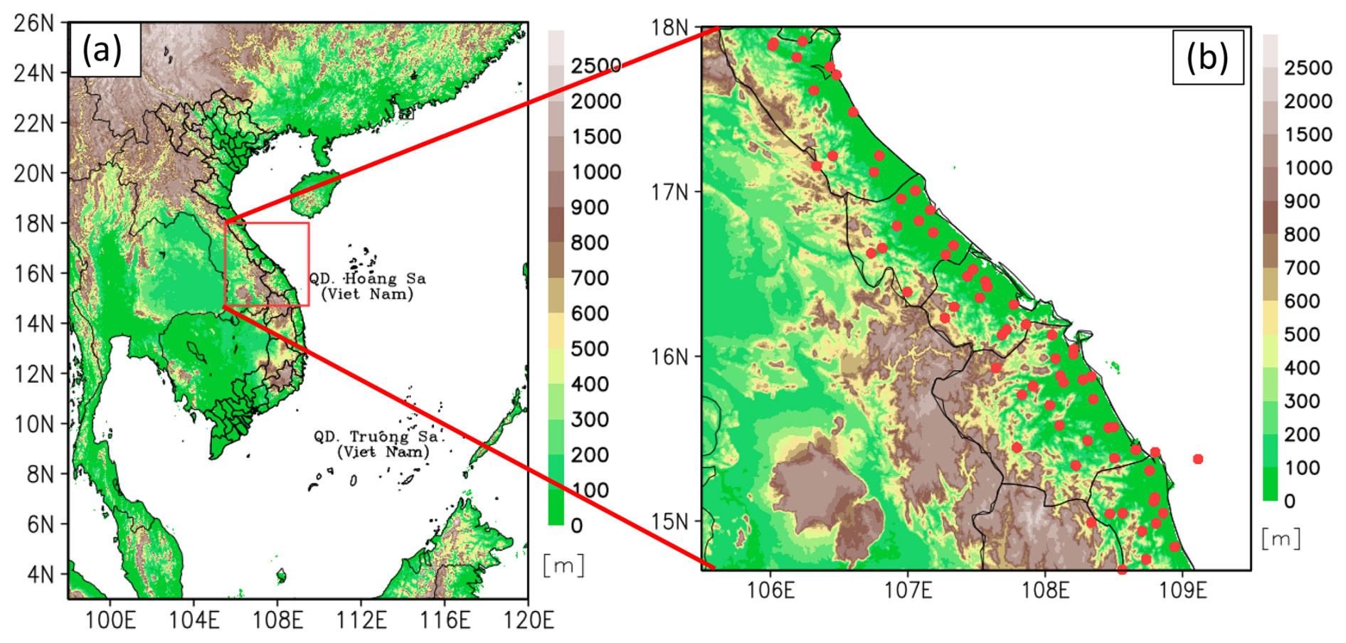
Figure 2 (a) The simulation domain of the CReSS model and topography (m, shaded) used in the study. The red box marks the study area. (b) The distribution of the observation stations (red dots) in the study area.

The review above suggests that considerable limitations still exist in forecasting heavy rainfall in central Vietnam, especially using coarser models. It also indicates that a high-resolution time-lagged ensemble approach may offer some advantages in the prediction of extreme rainfall events, such as a better simulation of local weather conditions, a quicker response to changes in forecast uncertainty in real time, and potentially a longer lead time for hazard preparation. Climatologically, the whole of Vietnam lies in the tropical zone (Fig. 2a), where vigorous but less organized convection often develops in response to local conditions. This region is also prone to the influence and interactions of weather systems spanning a wide range of scales as reviewed. In addition, although central Vietnam is a small region with the narrowest place only about 80 km in width, it possesses significant topography running in the north–south direction that significantly affects rainfall (Fig. 2a). Hence, a high-resolution CRM with detailed and explicit treatment in cloud microphysics is likely crucial for better QPFs for heavy rainfall in central Vietnam.

Given the above review and analysis, the following scientific hypotheses are proposed: storm-scale processes and convection were important in the D18 event. However, both global and mesoscale models with a grid size down to 6 km × 6 km are not good enough for heavy-rainfall QPF without cloud-resolving capability (Fig. 1). Therefore, it is hypothesized that at higher resolution, the cloud-resolving time-lagged ensemble system (using the CReSS model) can improve the QPFs of this event in the short range. Additionally, this approach may also be able to extend the lead time of decent QPF beyond the short range. So, the goals of the study are to (1) examine the hypothesis above; (2) investigate the (practical) predictability of this event through a series of time-lagged ensemble predictions, including whether a decent QPF can be made at a longer lead time; and (3) identify important factors leading to this event, including the lead time of the signals of these factors, using the ESA method. The rest of this paper is organized as follows. Section 2 describes the data, model, and methodology used in the study. The model results are presented and evaluated in Sect. 3. Finally, conclusions are offered in Sect. 4.

2 Data and methodology

2.1 Data

2.1.1 Model validation

In situ observation data

The daily in situ rainfall observations (12:00–12:00 UTC, i.e. 19:00–19:00 LST) from 8 to 12 December 2018 at 69 automated gauge stations across central Vietnam are used for case overview and verification of model results. This dataset is provided by the Mid-Central Regional Hydro Meteorological Center, Vietnam. The spatial distribution of these gauge stations is depicted in Fig. 2b.

The Global Precipitation Measurement (IMERG Final Run V07) data

Global Precipitation Measurement (GPM) is a joint international mission between the National Aeronautics and Space Administration (NASA) and the Japan Aerospace Exploration Agency (JAXA), employing a satellite network for advanced global rain and snow observations. The GPM IMERG Final Run is a research-level product which is created by intercalibrating, merging, and interpolating “all” satellite microwave precipitation estimates along with microwave-calibrated infrared (IR) satellite estimates, analyses from precipitation gauges, and potentially other precipitation estimation methodologies at fine spatial and temporal scales. The horizontal resolution of this dataset is 0.1° × 0.1° latitude–longitude, and the time interval is every 30 min (Huffman et al., 2020). In this study, we used these satellite data (version 7) to verify rainfall distribution over the coastal sea due to the limitation of the gauge network, where observations exist only inland as shown in Fig. 2b. The GPM IMERG data span 12:00 UTC on 8 December to 12:00 UTC on 11 December 2018 and are used to analyse the D18 event as well as the rainiest day of this event (10 December).

The NCEP GDAS/FNL global tropospheric analyses data

The present study used this dataset (version d083003) to verify initial data and model outputs. The NCEP FNL analysis is an operational global gridded analysis and is freely provided by the NCEP. The horizontal resolution of this dataset is 0.25° × 0.25° latitude–longitude with 26 levels extending from the surface to 10 hPa. The temporal interval is 6 h. The variables used in this study include the zonal and meridional wind components, relative humidity, and vertical velocity at 925 hPa covering the case period from 18:00 UTC on 4 December to 12:00 UTC on 9 December 2018.

2.1.2 The added values of CReSS ensemble

The International Grand Global Ensemble retrieval

In this study, we used the global model predictions to analyse the predictability of the D18 event. The International Grand Global Ensemble (TIGGE) is a key component of The Observing System Research and Predictability Experiment (THORPEX) research programme, whose aim is to accelerate the improvements in the accuracy of 1 d to 2-week high-impact weather forecasts. The TIGGE provides not only deterministic forecast data but also ensemble prediction datasets from major centres, including NCEP of the USA, ECMWF of European countries, and JMA of Japan, with data going back to 2006. The TIGGE dataset has been used for a wide range of research studies on predictability and dynamical processes. The variables utilized included total precipitation and surface winds (at 10 m height) from NCEP, ECMWF, and JMA at 6 h intervals during the data period from 12:00 UTC on 8 December to 12:00 UTC on 11 December 2018 (as shown in Fig. 1a–c). The link to this dataset is placed in the “Code and data availability” section.

2.2 Model description and experiment setup

We used the Cloud-resolving Storm Simulator (CReSS) developed by Nagoya University, Japan (Tsuboki and Sakakibara, 2002, 2007). This is a non-hydrostatic and compressible cloud model, designed for simulation of various weather events at high (cloud-resolving) resolution. In the model, the cloud microphysics is treated explicitly at the user-selected degree of complexity, such as the bulk cold-rain scheme with six species: vapour, cloud water, cloud ice, rain, snow, and graupel (Lin et al., 1983; Cotton et al., 1986; Murakami, 1990; Murakami et al., 1994; Ikawa and Saito, 1991). Other subgrid-scale processes parameterized, such as turbulent mixing in the planetary boundary layer and physical options for surface processes, including momentum/energy fluxes and shortwave and longwave radiation, are summarized in Table 1.

Table 1 The basic information of experiments.

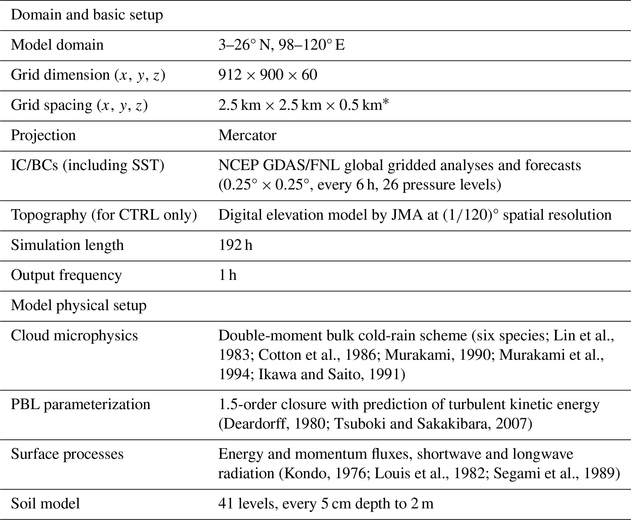
^∗ The vertical grid spacing (Δz) of CReSS is stretched (smallest at bottom), and the averaged value is given in parentheses.

For the initial condition (IC) and boundary conditions (BCs), the NCEP GFS analyses and deterministic forecast runs, executed every 6 h at 00:00, 06:00, 12:00, and 18:00 UTC daily (dataset d084001), were used to drive the CReSS model predictions. The horizontal resolution of the data is 0.25° × 0.25°, with 26 vertical levels, and the forecast fields are provided every 3 h from the initial time out to a range of 192 h. The data link is also placed in the “Code and data availability” section.

To evaluate of the predictability of the D18 event using an ensemble time-lagged high-resolution system and investigate the ensemble sensitivity of variables for the rainfall, 29 experiments were performed. The first member was initialized at 12:00 UTC on 3 December and the last one at 12:00 UTC on 10 December 2018. Between them, a new member was initialized every 6 h and all members have a simulation length of 192 h. All experiments used a single domain at 2.5 km horizontal grid spacing and a dimension in (x, y, z) of 912 × 900 × 60 grid points (Table 1; see Fig. 2). As mentioned above, the NCEP GFS was used as the IC/BCs of the CReSS model.

2.3 Verification of model rainfall

In order to verify model-simulated rainfall, some verification methods are used, including (1) visual comparison between the model and the observation (from the 69 automated gauges over the study area) and (2) objective verification using categorical skill scores at various rainfall thresholds from the lowest at 0.05 mm up to 900 mm for 3 d total. These scores are presented below along with their formulas and interpretation. To apply these scores at a given threshold, the model and observed value pairs at all verification points N (gauge sites here) are first compared and classified to construct a 2 × 2 contingency table (Wilks, 2006). At any given site, if the event takes place (reaching the threshold) in both model and observation, the prediction is considered a hit (H). If the event occurs only in observation but not the model, it is a miss (M). If the event is predicted in the model but not observed, it is a false alarm (FA). Finally, if both model and observation show no event, the outcome is correct rejection (CR). After all the points are classified into the above four categories, the categorical scores can be calculated by their corresponding formula as

$$\begin{array}{}\text{(1)}& {\displaystyle }\text{bias score (BS)}=(H+\mathrm{FA})/(H+M),\text{(2)}& {\displaystyle }\text{probability of detection (POD)}=H/(H+M),\text{(3)}& {\displaystyle }\text{false alarm ratio (FAR)}=\mathrm{FA}/(H+\mathrm{FA}),\text{(4)}& {\displaystyle }\text{threat score (TS)}=H/(H+M+\mathrm{FA}).\end{array}$$

The values of TS, POD, and FAR all range from 0 to 1, and the higher the better for both TS and POD, but the opposite is the case for FAR. For BS, its possible value can vary from 0 to N and indicate overestimation (underestimation) by the model for the events if greater than (less than) unity.

2.3.1 The similarity skill score

In addition to the categorical scores, the similarity skill score (SSS; Wang et al., 2022) is also applied to evaluate the model rainfall results, as

$$\begin{array}{}\text{(5)}& \mathrm{SSS}=\mathrm{1}-{\displaystyle \frac{\frac{\mathrm{1}}{N}\sum _{i=\mathrm{1}}^N(F_i-O_i{)}^{\mathrm{2}}}{\frac{\mathrm{1}}{N}\sum _{i=\mathrm{1}}^N{F}_i^{\mathrm{2}}+\frac{\mathrm{1}}{N}\sum _{i=\mathrm{1}}^N{O}_i^{\mathrm{2}}}},\end{array}$$

where N is the total number of verification points as before and F_i is the forecast rainfall amount and O_i the observed value at the ith point among N. The SSS is a measure against the worst mean squared error (MSE) possible. The formula shows that a forecast with perfect skill has an SSS of 1, while a score of 0 means zero skill when the model rainfall does not overlap with the observation anywhere.

Note that even though Eq. (5) has the same form as the fractions skill score (Roberts and Lean, 2008), the SSS is not a neighbourhood method. Thus, it is suited for QPF verifications where the rainfall location is important (as in our case).

2.3.2 The ensemble spread (standard deviation)

The ensemble spread is a measure of the difference among the members about the ensemble mean, and one suitable parameter is the standard deviation (SD). In other words, the ensemble spread reflects the diversity of all possible outcomes. Hence, the ensemble spread is often applied to describe the magnitude of the forecast errors. For a well-calibrated ensemble, for example, a small spread indicates high theoretical forecast accuracy (and low uncertainty), and vice versa for a large spread (Cattoën et al., 2020). Using the SD, the spread is computed by the formula below:

$$\begin{array}{}\text{(6)}& \mathrm{SD}=\sqrt{{\displaystyle \frac{{\sum }_{i=\mathrm{1}}^n(x_i-{\mathit{\mu }}_x{)}^{\mathrm{2}}}{n-\mathrm{1}}}},\end{array}$$

where x_i is the predicted value of member i for the variable x, μ_x is the ensemble mean, and n is the total number of ensemble members.

2.3.3 Ensemble sensitivity analysis

As mentioned above, an ensemble forecast is a set of forecasts produced by many separate forecasts typically with different initial conditions. Moreover, as we know, NWP outcomes are often sensitive to small changes in ICs and the sensitivity analysis is considered a method to improve forecasts through targeting observations. Hence, this study used the ESA method introduced by Ancell and Hakim (2007) to examine how a forecast variable responds to changes in ICs. The ensemble sensitivity is computed by the following formula:

$$\begin{array}{}\text{(7)}& {\displaystyle \frac{\partial R}{\partial x_t}}={\displaystyle \frac{\mathrm{COV}(R,x_t)}{\mathrm{VAR}\left(x_t\right)}}.\end{array}$$

Here, the response function R is chosen to be the areal-mean 24 h accumulated rainfall in central Vietnam (15.5–16.3° N, 107.9–108.6° E) on the rainiest day, from 12:00 UTC on 9 December to 12:00 UTC on 10 December 2018. The starting time of this period, i.e. 12:00 UTC on 9 December, is defined as t₀. Various scalar variables are considered for x_t, at a time from 48 h earlier (t₋₄₈, or 12:00 UTC on 7 December) to t₀ at 24 h intervals. The COV is the covariance of R and x_t, and VAR is the variance of x_t.

Since the analysis in Part 1 has identified that the D18 event was caused by the combined effect between the atmospheric disturbances at lower levels, such as the cold surge and easterly wind, and the topography, the ESA herein has been applied to selected variables at surface, near-surface, and mid-tropospheric levels to assess the sensitivity of the rainfall field to ICs and its predictability. In order to facilitate the comparison among the impacts of different variables, this study normalized ESA results using the standardized anomaly in the denominator of Eq. (7) and expressed them as the change in R (in mm) in response to an increase in x_t by 1 SD in subsequent sections.

3 Model results

3.1 Time-lagged 24 h QPFs by the CReSS model

In this section, time-lagged forecasts targeted for the 24 h period from 12:00 UTC on 9 December to 12:00 UTC on 10 December in the D18 event by the 2.5 km CReSS model are presented and evaluated. This 24 h period is chosen because it is the rainiest day with in situ observation exceeding 600 mm at some stations (Fig. 3 “OBS”). Figure 3 shows 25 possible scenarios of 24 h rainfall and average surface winds over the target period produced by the lagged runs every 6 h, with the earliest initial time at 12:00 UTC on 3 December and the latest one at 12:00 UTC on 9 December 2018. It is immediately clear that several members made a rather good 24 h QPF not only in amounts, but also in rainfall location and spatial distribution. These include most members starting during 8–9 December and also an impressive member from 18:00 UTC on 4 December. In this latter run, a reasonably good QPF was produced at a rather long lead time, almost 5 d (114 h) prior to the beginning of the target period. A common feature among these good members is that they all captured the direction and magnitude of surface winds quite well. On the other hand, most other members were less ideal in their QPFs when initialized before 06:00 UTC on 7 December at lead times beyond 2 d (before the target period). In general, they also did not predict the surface winds well enough.

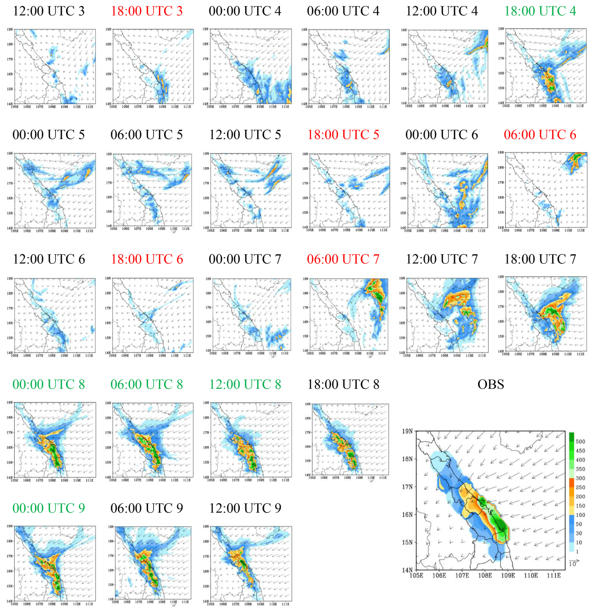
Figure 3 The predicted 24 h accumulated rainfall (mm, shaded, scale on the right of panel OBS) and the mean surface horizontal wind (m s⁻¹, vector, reference length at panel OBS) on 10 December 2018 (from 12:00 UTC on 9 December to 12:00 UTC on 10 December 2018). The green colour marks good members, and the red colour marks bad members. In OBS, 24 h in situ-observed rainfall (mm, shaded) and the surface wind derived from ERA5 data (m s⁻¹, vector) are shown, adapted from Fig. 12f of Wang and Nguyen (2023).

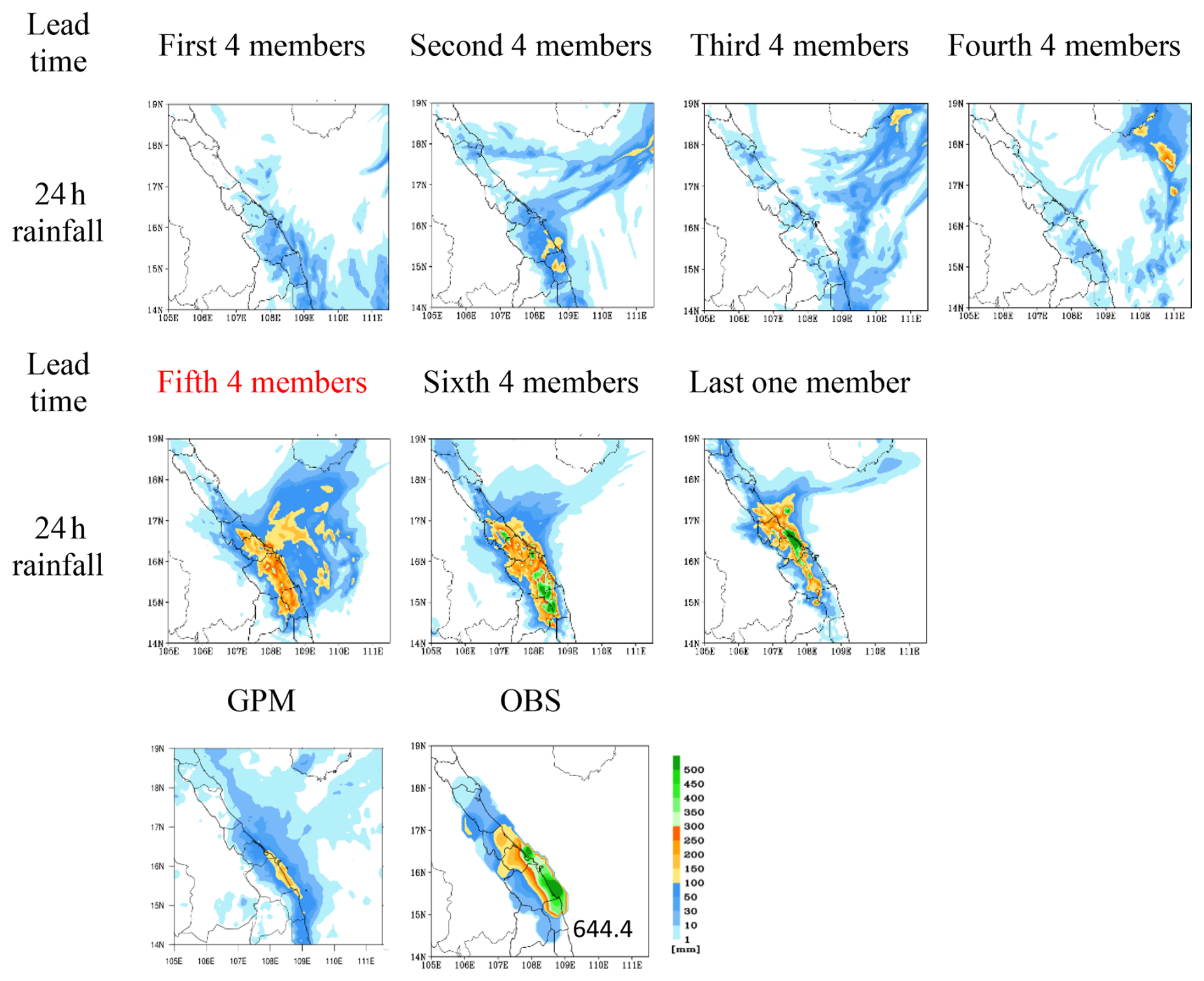
Figure 4 The predicted 24 h rainfall by subgroup members, 24 h accumulated rainfall by the Global Precipitation Measurement (GPM) estimate (IMERG Final Run product), and 24 h observed rainfall (mm, peak amount labelled at the lower-right corner) for the period of 12:00 UTC on 9 December–12:00 UTC on 10 December 2018 as labelled. The same colour bar (lower right) is used for all panels.

Furthermore, as we know, ensemble weather forecasts are a set of forecasts from multiple members that represent the range of future weather possibilities, and the simplest way to use them is through the ensemble mean, which emphasizes the features that the members agree upon. In order to see how well the 2.5 km CReSS can predict the D18 event with the time-lagged strategy in terms of possible scenarios of 24 h accumulated rainfall for 10 December, lagged runs are grouped based on their range of initial times in Fig. 4. It can be clearly seen that the rainfall predictions by the fifth group of four (executed between 12:00 UTC on 7 December and 06:00 UTC on 8 December) and the sixth group of four members (between 12:00 UTC on 8 December and 06:00 UTC on 9 December) are quite similar to the observation, not only in rainfall amount but also in the locations of concentrated rainfall. For other subgroups, the rainfall was much lower than the observation in their scenarios. The rainfall accumulations from the third (12:00 UTC on 5 December to 06:00 UTC on 6 December) and fourth groups of four (12:00 UTC on 6 December to 06:00 UTC on 7 December) members are the lowest. One assessment relevant to the outcome of these eight runs is that none of them predicted the surface wind field well enough in their ranges (beyond 3 d), as discussed previously. On the other hand, the mean rainfall from the second group of four members (12:00 UTC on 4 December to 06:00 UTC on 5 December) is the best among all subgroups in the extended range due to a single good forecast initialized at 18:00 UTC on 4 December (see Fig. 3 (18:00 UTC on 4 December)).

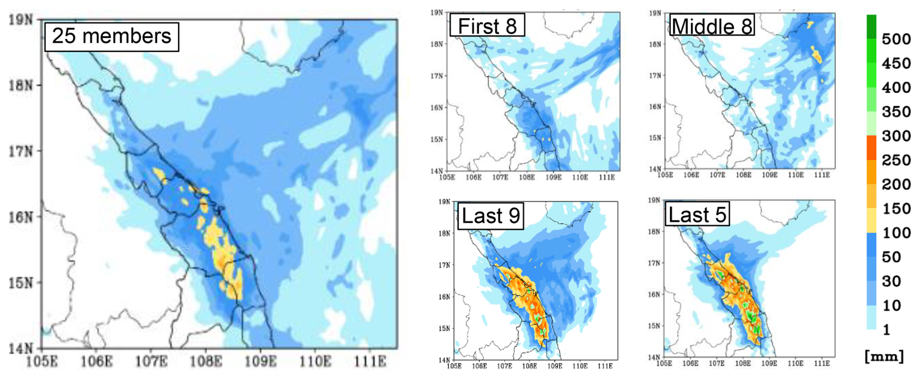
Figure 5 Ensemble mean rainfall (shaded, scale on the right) from all 25 time-lagged members, executed every 6 h from 12:00 UTC on 3 December to 12:00 UTC on 9 December, for the 24 h period from 12:00 UTC on 9 December to 12:00 UTC on 10 December.

Besides the evaluation on time-lagged results using batches of successive runs (every four members) as presented above, this study also grouped the members using different ensemble sizes based on their behaviour in order to better assess the temporal evolution of forecast uncertainty and event predictability as the lead time shortened. Particularly, the 25 members were divided into several subgroups as shown in Fig. 5, including the first eight members (those executed during 12:00 UTC on 3 December–06:00 UTC on 5 December), the middle eight members (runs between 12:00 UTC on 5 December and 06:00 UTC on 7 December), the last nine members (12:00 UTC on 7 December–12:00 UTC on 9 December), and the last five members (12:00 UTC on 8 December–12:00 UTC on 9 December). In other words, the last five members were those executed within 24 h (1 d) prior to the beginning of the target period and so on.

In Fig. 5, it is clear that both the ensemble means from the last five and the last nine members compare quite favourably to the observation, not only in the accumulated amount but also in the spatial distribution of rainfall. This indicates that the model could produce QPFs at fairly good quality and rather consistently since the time as early as roughly 48 h prior to the commencement of the rainfall event (also Fig. 3). These two subgroups within the short range gave much better quality in QPFs than the other subgroups executed before them at longer lead times, including the first eight, middle eight, and all 25 members.

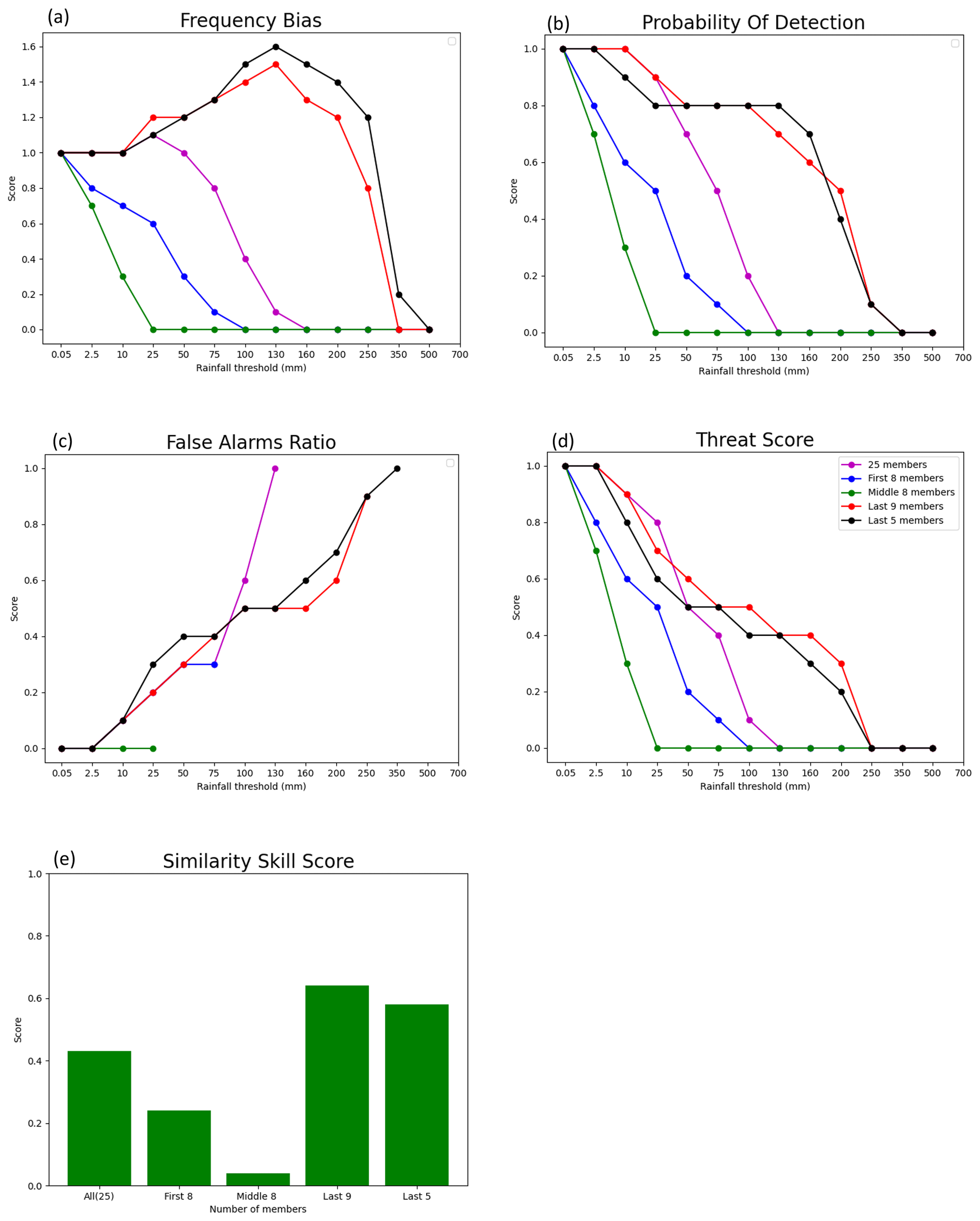
Figure 6 Statistic scores for 24 h mean rainfall, obtained from 25 members of the 8 d forecasts for 10 December 2018 (from 12:00 UTC on 9 December to 12:00 UTC on 10 December).

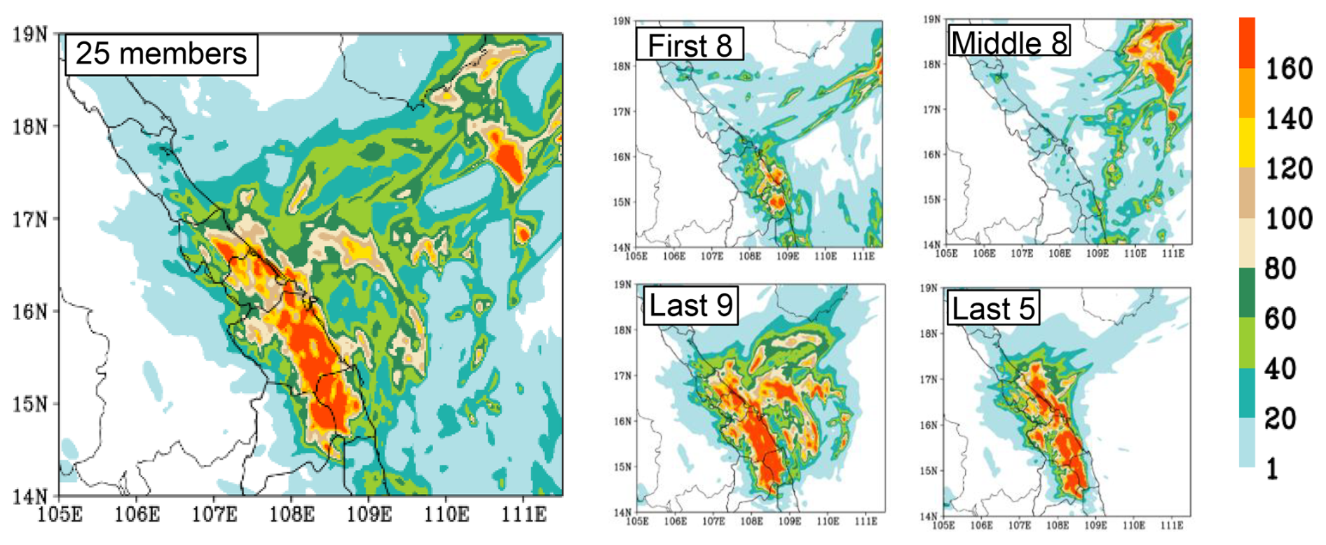
Figure 7 The spread (shaded, scale on the right) from all 25 time-lagged members, executed every 6 h from 12:00 UTC on 3 December to 12:00 UTC on 9 December, for the 24 h period from 12:00 UTC on 9 December to 12:00 UTC on 10 December.

In terms of skill scores, for example, the mean QPFs by the last five members have TS = 0.4, POD = 0.8, BS = 1.5, and FAR = 0.5 at 100 mm (per 24 h), while the last nine members give similar scores of TS = 0.5, POD = 0.8, BS = 1.4, and FAR = 0.5 (Fig. 6a–d). On the contrary, the mean QPFs from both the first and middle eight members only yield zero scores in TS, POD, and BS with no skill in FAR at 100 mm (and above), obviously due to not enough rainfall in central Vietnam in most of their members. At 200 mm (per 24 h), similarly, the last five members (TS = 0.2, POD = 0.4, BS = 1.4, and FAR = 0.7) and the last nine members (TS = 0.3, POD = 0.5, BS = 1.2, and FAR = 0.6) again produce much better scores in QPFs, compared to no skill in all four scores in QPFs from the middle eight, first eight, and all 25 members (Fig. 6a–d). In SSS, the mean from the last nine members exhibits the highest score (0.64), the middle eight members have the lowest score (0.04), and the mean from all 25 members is 0.43 (Fig. 6e).

However, as indicated by the SD, the spreads in rainfall scenarios in both ensembles from the last five and nine members are quite large (Fig. 7). Thus, while the lagged members can produce a wide range of possible rainfall scenarios for the D18 event, which is the main purpose of an ensemble as reviewed in Sect. 1, the members often cannot agree on the precise locations of heavy rainfall. Given the small scale of local convection during the event, this result is perhaps anticipated. On the other hand, the maxima in spread are > 160 mm in Fig. 7 among the last nine members, which is perhaps quite reasonable in magnitude compared to the peak amounts of about 400 mm in the ensemble mean. In any case, Figs. 6 and 7 indicate that the predictability of the D18 event changed considerably with time, and the 2.5 km CReSS has a good skill in QPFs inside the short range (≤ 72 h). However, it remains difficult to predict the event successfully at longer lead times.

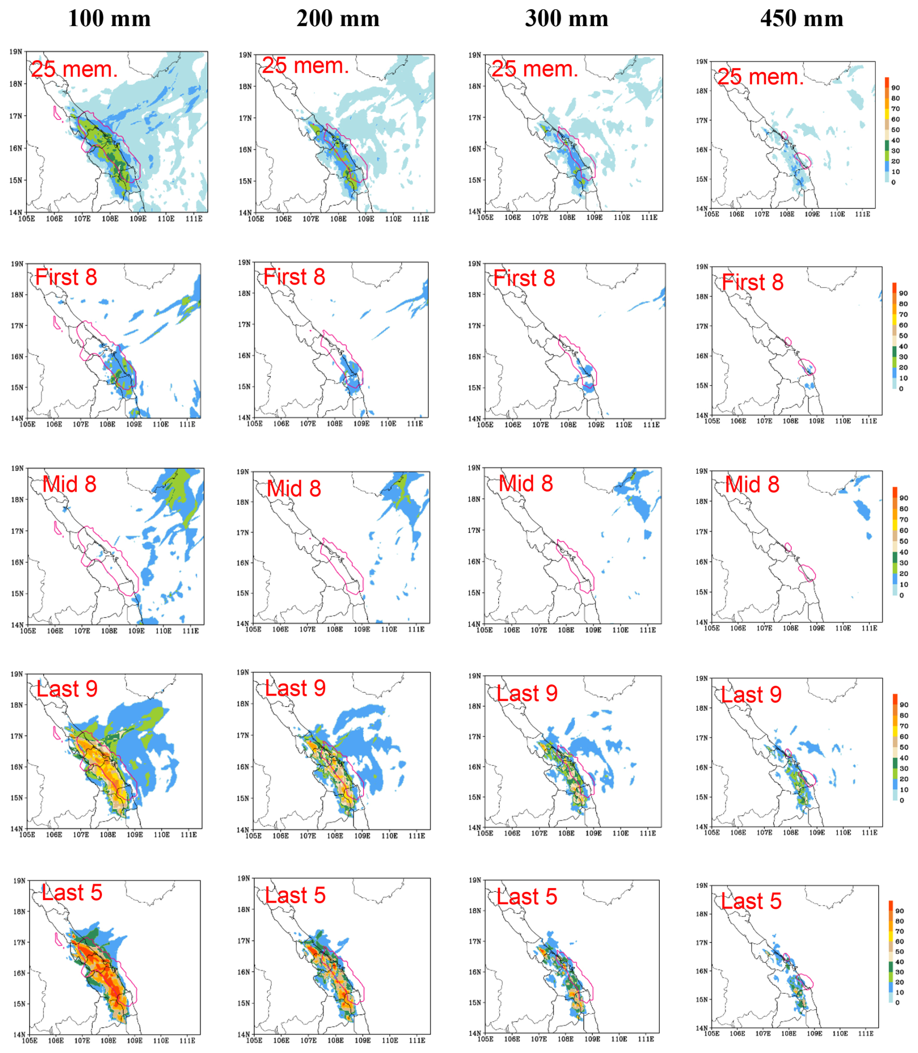
Figure 8 Probability distribution (%; shaded, scale on the right) from all 25 time-lagged members, executed every 6 h from 12:00 UTC on 3 December to 12:00 UTC on 9 December, reaching thresholds of 100, 200, 300, and 450 mm, for the 24 h period from 12:00 UTC on 9 December to 12:00 UTC on 10 December. The observed areas at the same thresholds are depicted by the pink contours. For each panel, the red label in the top-left corner shows the number of members grouped to calculate the probability distribution.

The probability information derived from the sub-ensemble groups at four different rainfall thresholds from 100 to 450 mm is shown in Fig. 8, in which the increase in heavy-rainfall probability in central Vietnam and thus also the predictability of the event with time are evident. From the first eight members executed in the longest range (≥ 102 h prior to rainfall accumulation), there is only a 10 %–25 % chance in parts of central Vietnam of receiving at least 100 mm of rainfall for 10 December (from 12:00 UTC on 9 December to 12:00 UTC on 10 December). The probability is even lower from the middle eight members (run between 54–96 h prior to target period), as their SSS is the lowest among all sub-ensemble groups and only a couple of the runs could reach 100 mm anywhere inland in central Vietnam. As the lead time shortens to inside the short range, the probabilities of having ≥ 100 mm of rainfall increase dramatically, to roughly 70 %–80 % in the last nine members and further to over 80 %–90 % in the last five members. Due to the contribution from later members, about 20 %–40 % of all 25 members can reach 100 mm inland. Toward higher thresholds, the probabilities decrease in Fig. 8 as expected, and so do the areal sizes actually reaching those thresholds (pink contours). At the highest value of 450 mm, the ensembles in general show less than about a 20 %–30 % chance for its occurrence from the last five and last nine members, respectively, and the high-probability areas are also slightly more inland than the observed one.

3.2 Ensemble-based sensitivity analysis

The results in Sect. 3.1 above reveal that the CReSS model with a horizontal grid size of 2.5 km predicted good QPFs for the rainiest day of the event and performed better than those reviewed in Sect. 1. Therefore, relying on this good performance, the ESA is carried out in this subsection.

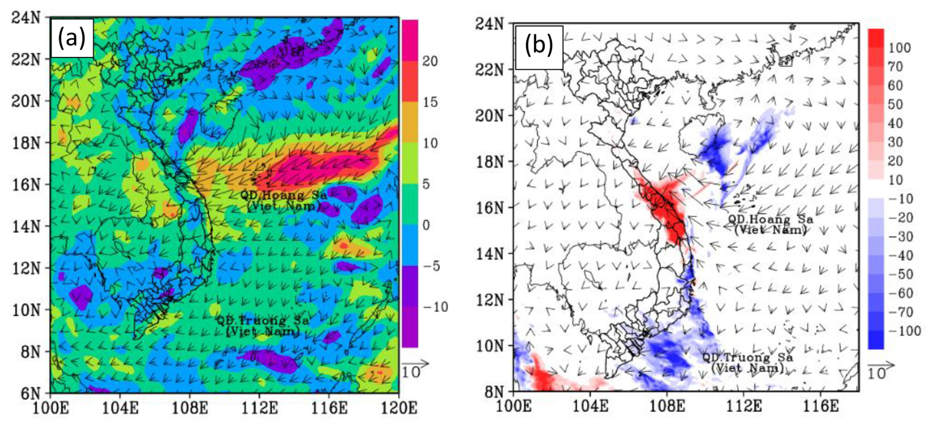
Figure 9 The difference in (a) input data (boundary conditions) and (b) CReSS output between averaged five good members (members ran at 18:00 UTC on 4 December, 00:00 UTC on 8 December, 06:00 UTC on 8 December, 12:00 UTC on 8 December, 00:00 UTC on 9 December) and five bad members (members ran at 18:00 UTC on 3 December, 18:00 UTC on 5 December, 06:00 UTC on 6 December, 18:00 UTC on 6 December, 06:00 UTC on 7 December). For input data, relative humidity (%, shaded) and surface wind (m s⁻¹, vector) are shown for 12:00 UTC on 9 December 2018. For CReSS output, 24 h accumulated rainfall (mm, shaded) and surface wind (m s⁻¹, vector) are shown.

Firstly, five good members (those with initial times at 18:00 UTC on 4 December; 00:00, 06:00, and 12:00 UTC on 8 December; and 00:00 UTC on 9 December) and five bad ones (those ran at 18:00 UTC on 3 December, 18:00 UTC on 5 December, 06:00 and 18:00 UTC on 6 December, and 06:00 UTC on 7 December) are chosen, and by using their differences (good minus bad members), Fig. 9 shows that the main reason for the significantly different forecast outcomes lies in differences in the input datasets (i.e. IC/BCs). Specifically, the surface easterly winds were much stronger and the relative humidity much higher surrounding central Vietnam and its upstream areas in the GFS forecast data valid at 12:00 UTC on 9 December (used as BCs in CReSS runs) in the good members compared to the bad ones (Fig. 9a). Subsequently, the good CReSS members produced much more rainfall in central Vietnam (Fig. 9b). These factors were also identified as crucial for the extreme rainfall in the D18 event in Part 1.

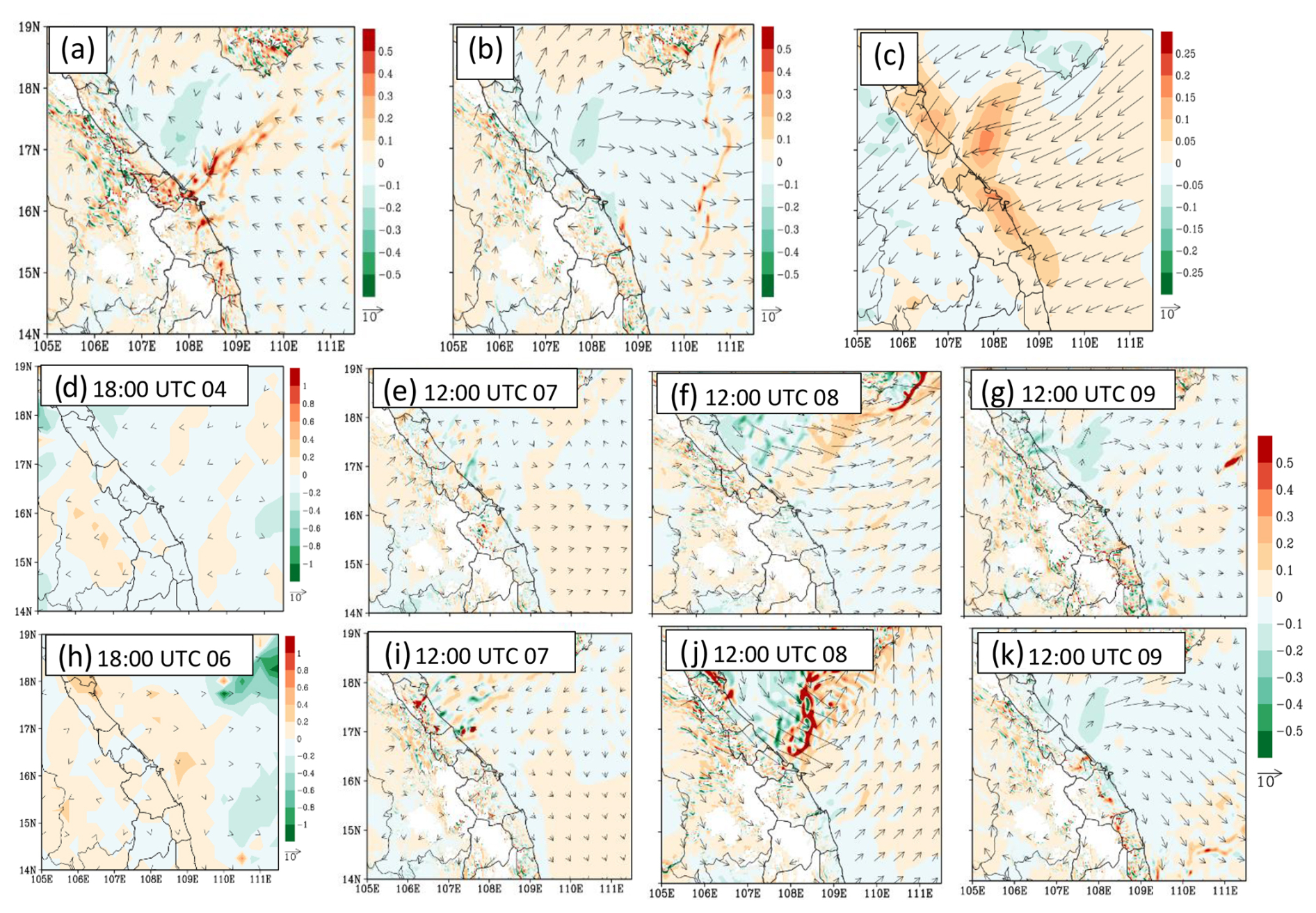
Figure 10 The difference in the horizontal wind (m s⁻¹, vector, reference length at the lower-right corner of the panel), and vertical velocity (m s⁻¹, shaded, the reference colour scale is on the right of panel) between the (a) averaged five good members and (b) averaged five bad members and the NCEP FNL analysis data at 925 hPa and at 12:00 UTC on 9 December​​​​​​​. (c) The NCEP FNL analysis horizontal wind (m s⁻¹, vector, reference length at the lower-right corner of the panel) and vertical velocity (m s⁻¹, shaded) at 925 hPa​​​​​​​ and at 12:00 UTC on 9 December. (d) The difference in the horizontal wind (m s⁻¹, vector, reference length at the lower-right corner of the panel) and relative humidity (%, shaded; the reference colour scale is on the right of panel) between the initial data of a good member at a longer lead time (at 18:00 UTC on 4 December) and the NCEP FNL analysis data at 925 hPa. Panels (e), (f), and (g) present the difference in the evolution of weather features with time by this good member. (h) As in panel (d) but for a bad member (member ran at 18:00 UTC on 6 December). (i, j, k) As in panels (e), (f), and (g), respectively, but for the abovementioned bad member. Compared variables are horizontal wind at 925 hPa (m s⁻¹, vector, reference length at the lower-right corner of the panel) and vertical velocity (m s⁻¹, shaded, the reference colour scale is on the right of panel). The NCEP FNL analysis gives horizontal wind (m s⁻¹, vector, reference length at the lower-right corner of the panel) and vertical velocity (m s⁻¹, shaded) at 925 hPa.

Meanwhile, Fig. 10 shows the difference in the evolution of synoptic-scale patterns (features) zoomed into the study area. To be more specific, Fig. 10a depicts the difference (CReSS output minus NCEP FNL analysis) in the horizontal wind and vertical velocity between the averages of the five good members and the NCEP FNL analysis at 925 hPa at 12:00 UTC on 9 December, and it is small although each member was initialized at a different lead time. This implies that these members captured the evolution of weather patterns of this event well. Additionally, the model vertical velocity is seen to be stronger than that of the NCEP FNL data. Therefore, these members produced the rainfall closer to the observation with the presence of complex terrain in the study area. On the contrary, bad members did not capture the evolution of weather patterns well enough (Fig. 10b), and they could not produce good QPFs as a result.

Furthermore, Fig. 10d indicates very small differences in the IC of the member that was initialized at 18:00 UTC on 4 December to the FNL analysis (thus suggesting smaller errors), especially over the study area. From these initial data, the evolution of weather patterns in this CReSS run also agreed well with the analyses during the first 3 d (not shown), and the differences remained relatively small even at 12:00 UTC on 9 December, at a lead time of roughly 5 d (Fig. 10e, f, g). Compared to this, a bad member initialized at 18:00 UTC on 6 December (at a shorter lead time by 2 d) exhibited somewhat larger differences in the initial state in relation to the NCEP FNL analysis (Fig. 10h). This difference then led to larger and more evident differences in weather patterns, as seen in Fig. 10i, j, and k by this particular member that performed worse in QPFs (member ran at 18:00 UTC on 6 December). The results here not only indicate that it is still possible to have good rainfall forecasts at a lead time up to 5 d, but also show some predictability by a cloud-resolving model at such long lead times.

Additionally, the above results also reaffirm that very small differences in the initial data can lead to a vastly different outcome, especially as the forecast range increases, in extreme rainfall events (such as the D18 event) that involve highly nonlinear deep convection. As pointed out in Part 1, the low-level wind convergence led to moisture convergence, and these conditions played a crucial role in the D18 event. The southward movement of the low-level wind convergence also dictated the movement of the convective rainband during the event. Therefore, the ESA was applied to relevant variables, including the horizontal wind and mixing ratio of water vapour. The quantitative results are shown in Figs. 11–13 and presented below.

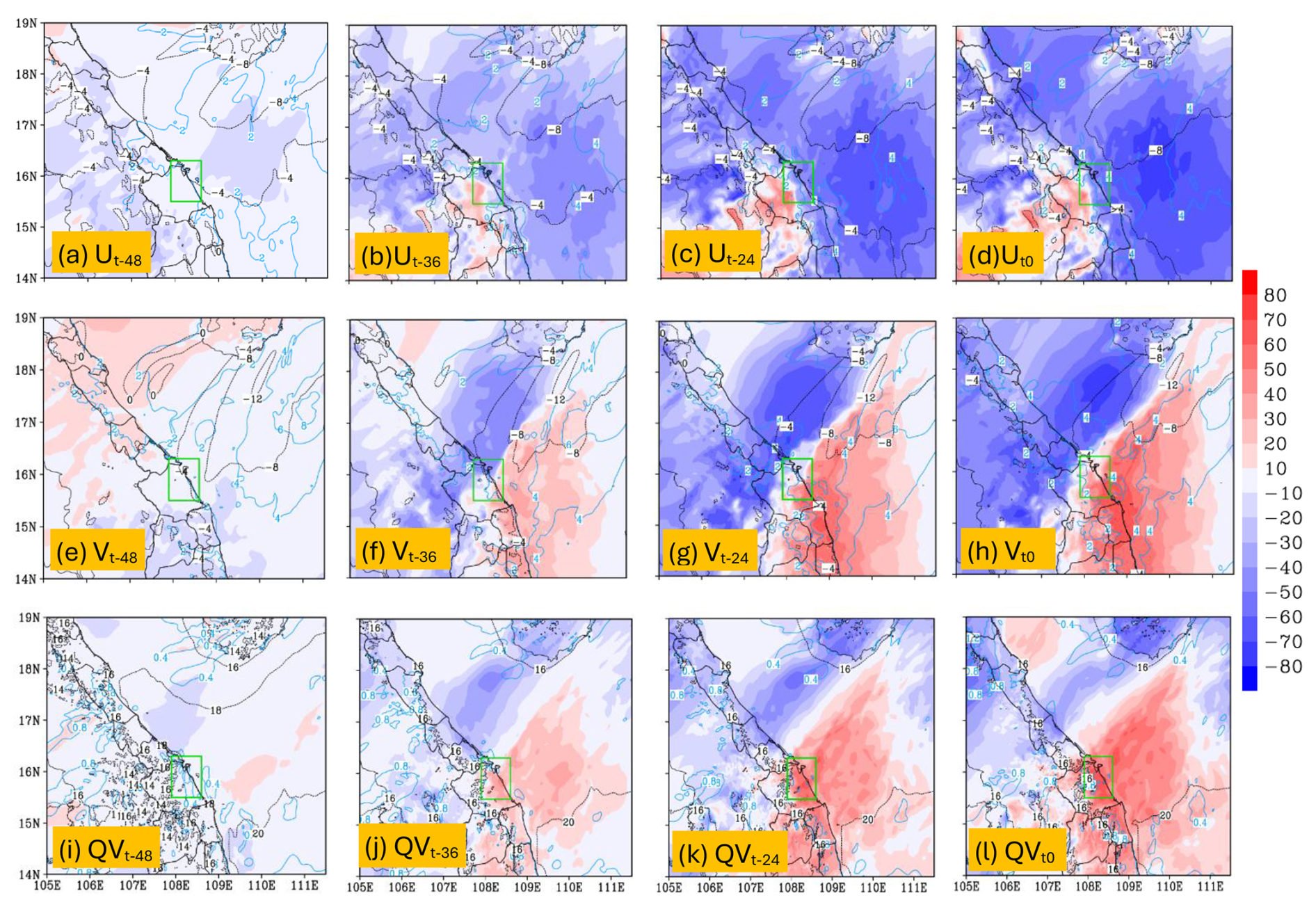
Figure 11 The sensitivity (mm, per SD, colour, scale on the right) of areal-mean 24 h accumulated rainfall in central Vietnam starting from t₀ (i.e. R, averaging area depicted in green box) to the surface wind components (m s⁻¹, shaded) and the ensemble mean (contours, every 4 m s⁻¹) and to surface water vapour mixing ratio (r, g kg⁻¹) and its ensemble mean (contours, every 0.06 g kg⁻¹) at different lead times from t₋₄₈ to t₀. The time of t₀ is 12:00 UTC on 9 December 2018. Panels (a)–(d) are for the zonal wind component, panels (e)–(h) for the meridional wind component, and panels (i)–(l) for surface water vapour mixing ratio. The standard deviation is exhibited by the mid-blue contours.

Figure 11 shows the sensitivity of mean 24 h total rainfall inside the green box in central Vietnam (R) to zonal (u) and meridional (v) wind components and water vapour mixing ratio (q_v) at the surface, with the ensemble mean also plotted. It is clear that the sensitivity of rainfall to these variables is lower for longer forecast ranges and becomes higher as the lead time shortens. Specifically, from 2 d before (t₋₄₈) to the starting time of the accumulation period (t₀), the sensitivity of rainfall to u wind over the SCS and along the coast of central Vietnam turned more negative, indicating heavier rainfall associated with stronger easterly winds (u < 0) near the surface, especially in areas immediately upstream toward t₀ (Fig. 11a–d). The rainfall's sensitivity to v wind leading to t₀, on the other hand, exhibited a dipole structure in pattern, with negative values to the north-northwest and positive values to the south-southeast across central Vietnam and the upstream ocean (Fig. 11e–h). This structure indicates a stronger confluence in northeasterly winds over the region in rainier members, consistent with the results in Part 1. In Fig. 11e–h, the increase in v wind just south of central Vietnam is particularly evident, from −10 mm per SD (SD = 2 m s⁻¹) at t₋₄₈ to over +70 mm per SD (SD = 2–4 m s⁻¹) at t₀. Thus, the precipitation amount over central Vietnam in the D18 event is highly sensitive to the strength and confluence of northeasterly winds near the surface in short-range forecasts. Similarly, the rainfall was also highly sensitive to the water vapour amount and its flux convergence (Fig. 11i–l).

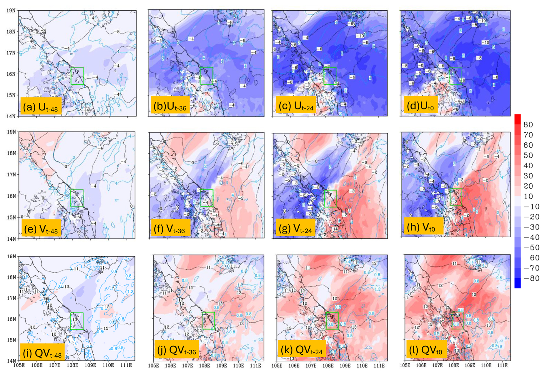
Figure 12 The sensitivity (mm, per SD, colour, scale on the right) of 24 h accumulated rainfall in central Vietnam starting from t₀ (i.e. R, averaging area depicted in green box) to the wind components (m s⁻¹, shaded) and the ensemble mean (contours, every 2 m s⁻¹) and to the water vapour mixing ratio (r, g kg⁻¹) and its ensemble mean (contours, every 0.4 g kg⁻¹) at an altitude of 1476 m and at different lead times from t₋₄₈ to t₀. The time of t₀ is 12:00 UTC on 9 December 2018. In which, panels (a)–(d) are for the zonal wind component, panels (e)–(h) for the meridional wind component, and panels (i)–(l) for the water vapour mixing ratio. The standard deviation is exhibited by the mid-blue contours.

Slightly higher up at 1476 m (near 850 hPa), where easterly flow prevailed during the D18 event (see Fig. 3b in Part 1), the sensitivity of rainfall to u and v winds exhibits similar spatial patterns (Fig. 12a–h) to those at the surface (Fig. 11a–h), with stronger easterly winds and a larger confluence in association with heavier rainfall. Similarly, the rainfall in central Vietnam is still highly sensitive to the mixing ratio at this level, both locally and over the surrounding area scale (Fig. 12i–l), again especially at shorter lead times. At the local scale, this positive correlation presumably is linked to upward transport of moisture, as the ascending motion in convective clouds could become larger at this level (and also more vigorous in rainier members).

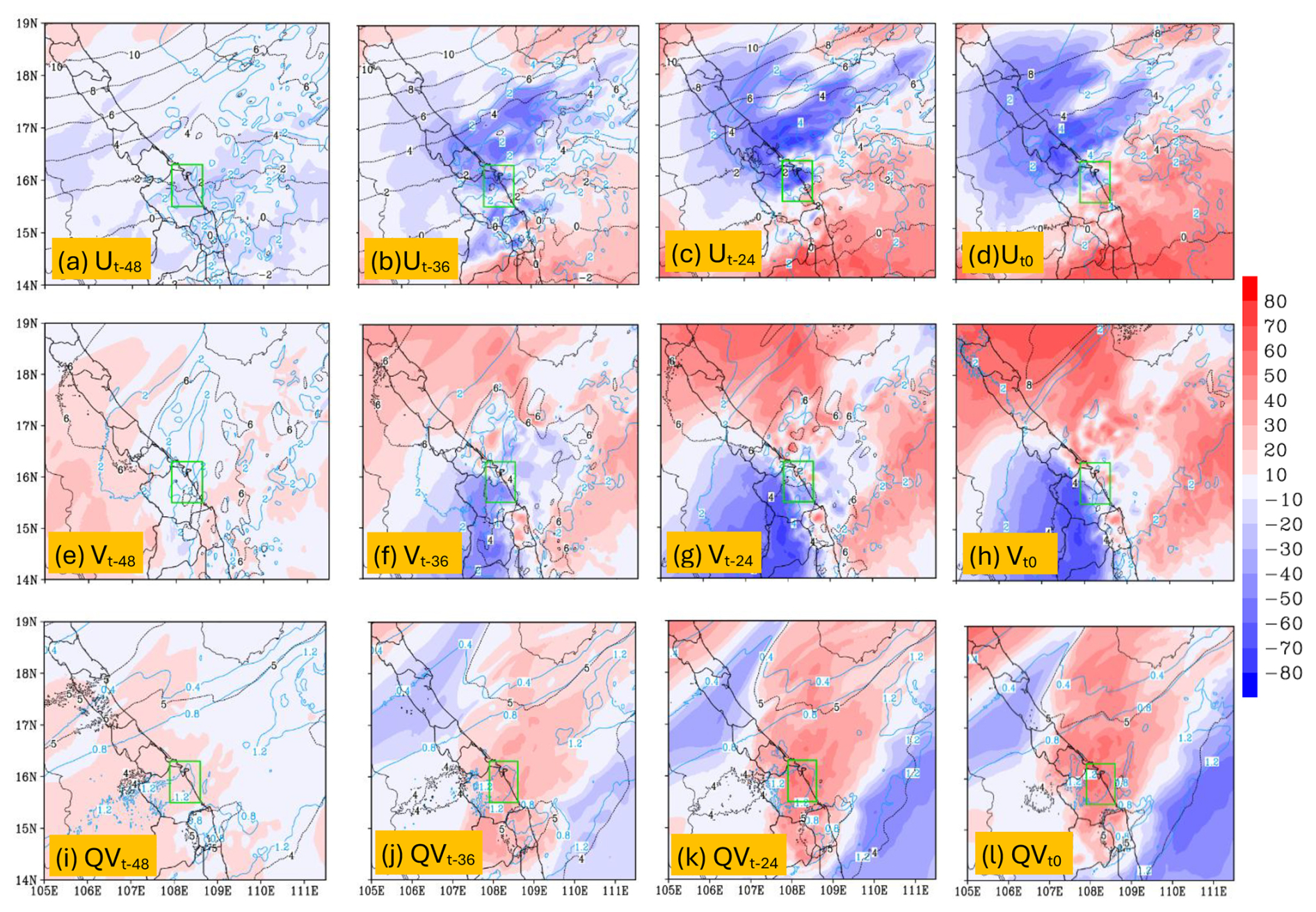
Figure 13 The sensitivity (mm, per SD, colour, scale on the right) of 24 h accumulated rainfall in central Vietnam starting from t₀ (i.e. R, averaging area depicted in green box) to the wind components (m s⁻¹, shaded) and the ensemble mean (contours, every 2 m s⁻¹) and to the water vapour mixing ratio (r, g kg⁻¹) and its ensemble mean (contours, every 0.4 g kg⁻¹) at an altitude of 5424 m and at different lead times from t₋₄₈ to t₀. The time of t₀ is 12:00 UTC on 9 December 2018. Panels (a)–(d) are for the zonal wind component, panels (e)–(h) for the meridional wind component, and panels (i)–(l) for the water vapour mixing ratio. The standard deviation is exhibited by the mid-blue contours.

At the upper level of 5424 m (near 500 hPa), it is seen that from t₋₄₈ to t₀, dipole structures developed in the sensitivity patterns of rainfall to both u and v winds (Fig. 13a–h). For u winds, positive sensitivity of up to about +70 mm per SD (SD = 2–4 m s⁻¹ depending on t) existed to the south, with negative values of up to −70 mm per SD (SD = 2–4 m s⁻¹) to the north of central Vietnam. Meanwhile, positive sensitivity to v wind appeared to the north and east with negative sensitivity to the south and west of the rainfall area. As the prevailing winds at 500 hPa were southeasterlies over southern Vietnam and southwesterlies over northern Vietnam during the D18 event (thus with anticyclonic curvature; see Fig. 3c in Part 1), the above sensitivity patterns, already apparent at t₋₂₄ (Fig. 13c, g), corresponded to stronger diffluence/divergence and a weaker anticyclone aloft to favour more rainfall. For q_v, positive sensitivity signals of up to +70 mm per SD (SD = 1.2 g kg⁻¹) also appeared over the rainfall area at t₋₂₄ and t₀ (Fig. 13i–l), and the reason for this is similar to that shown near 850 hPa in Fig. 12. Overall, the ESA performed in this study indicated clearly that the synoptic pattern that caused the D18 event had already developed at times more than 24 h earlier, and this explains why, with a high enough resolution and cloud-resolving capability, the CReSS forecasts could better predict and improve the QPFs inside the short range, as shown in this section.

4 Conclusion

As high resolution is required in numerical models to predict heavy rainfall more successfully, the present work utilizes a time-lagged high-resolution ensemble forecast system and evaluates how well the D18 event (during 9–12 December 2018) in central Vietnam can be predicted in advance before its occurrence. Using the CReSS model with a grid size of 2.5 km (912 × 900 grid points in the x and y dimensions with 60 vertical levels), ensemble forecasts were produced with a total of 29 time-lagged runs at 6 h intervals, each out to a forecast range of 192 h (8 d). Based on the goals raised from the analysis in Part 1, the key findings of this Part 2 study are summarized as follows.

The first goal of this study is regarding the scientific hypotheses that at a higher resolution, the cloud-resolving time-lagged ensemble can improve the QPFs of the D18 event in the short range and may also be able to extend the lead time of decent QPFs beyond the short range. Our evaluation results confirm that this strategy using the CReSS model can effectively improve the QPFs of this event in the short range. Furthermore, the results also demonstrate that a decent QPF for 10 December (the rainiest day) can be made at a longer lead time (initialized at 18:00 UTC on 4 December), when good initial conditions are provided.

Regarding the second goal, our investigation in predictability indicates that the 2.5 km system predicted the rainfall fields on 10 December during the event fairly well, including both the amount and the spatial distribution, within the short range at lead times of 1, 2, and 3 d. More specifically, the SSSs of QPFs for these three ranges are about 0.4, 0.6, and 0.7, respectively, with fairly consistent results among successive runs that indicate a reasonable predictability, despite some spread and disagreement regarding the precise locations of heavy rainfall. The above good results are due to the model's capability to better predict the conditions in the lower troposphere such as the wind fields.

At lead times longer than 3 d, however, the predictability of the event is lowered due to a higher level of forecast uncertainty, and the quality of QPFs drops with significant under-prediction. Nevertheless, good QPFs are still possible occasionally. At lead times beyond 6 d, it is challenging to achieve a good QPF at thresholds greater than 100 mm even with a high-resolution model. This is presumably linked to the rapid evolution of atmospheric conditions during such an extreme event surrounding Vietnam in a tropical environment. In the present study, a CRM is applied to forecast extreme rainfall in central Vietnam for the first time. Although still with certain limitations, our results do indicate that there is hope of predicting such events successfully beforehand, at least within the short range. Therefore, based on the present work, more studies on the predictability of extreme rainfall in Vietnam are recommended in the near future.

Regarding the third and final goal, ESA results show that the rainfall is most sensitive to the wind conditions in the lower troposphere leading up to the event, with more rain associated with stronger northeasterly to easterly winds and their confluence over central Vietnam (and the upstream region). Similarly, the rainfall also shows strong sensitivity to the moisture amount, not only at the surface but also further aloft at the upper levels. Besides, ESA also indicates that the synoptic pattern that caused the D18 event had already developed at a time earlier in the past. Furthermore, in the ESA, the finer-scale features (convection) are also seen to be linked to synoptic conditions in their background, implying that it is meaningful to apply ESA to control the perturbations in initial fields.

The key findings in this study underscore that both practical predictability and ESA are intertwined, influencing the design and evaluation of ensemble forecast systems, and are potentially applicable to other extreme rainfall events in the same season in Vietnam.