Groundwater recharge in Brandenburg is declining – but why?

Brandenburg is among the driest federal states in Germany, featuring low rates of groundwater recharge (GWR) across large parts of the state. This GWR is fundamental to both water supply and the support of natural ecosystems. There is strong observational evidence, however, that GWR has been declining since 1980: first, river discharge (which is almost exclusively fed via GWR) has been significantly decreasing in many catchments (by around 40 % since 1980). Second, groundwater levels in the groundwater recharge areas show a significant long-term decline. In this study, we search for potential reasons behind this decline by investigating five catchments across Brandenburg that we consider largely unaffected by direct anthropogenic interference with the water balance. Using the Soil-Water-Atmosphere-Plant (SWAP) model to simulate long-term trends in GWR, we found that significant increases in air temperature, solar irradiation, and leaf area index (LAI) since 1980 have acted towards a decrease in GWR on the order of −21 to −4 mm a⁻¹ per decade from 1980 to 2023. The Brandenburg-wide LAI trend of +0.1 m² m⁻² per decade was inferred from a recently published, spatio-temporally consistent LAI reconstruction. The contribution of this LAI trend to the decrease in GWR amounted to −5 to −3 mm a⁻¹ per decade. Based on our results, we consider it very likely that the decrease in discharge since 1980 can be explained by a decrease in GWR, which, in turn, was caused by climate change in combination with an increasing LAI. However, we also found that precipitation trends can be highly incoherent at the catchment scale. Even though these precipitation trends are not significant, they can have a fundamental impact on the significance, the magnitude, and even the sign of simulated GWR trends. Given the uncertainty in the precipitation trend, four out of five catchments still appear to exhibit a gap between negative simulated GWR trends and more negative observed discharge trends. We provide a comprehensive discussion of possible reasons and uncertainties to explain this gap, including the effects of the limited length and the inhomogeneity of climate and discharge records, the role of land cover and vegetation change, irrigation water consumption, latent anthropogenic interventions in the catchments' water balance, uncertainties in groundwater table depth, and model-related uncertainties. Addressing these uncertainties should be a prime subject for prospective research with regard to the effects of environmental change on GWR in Brandenburg. Water resource management and planning in Brandenburg should, however, already take into account the possibility of GWR decreasing further. Given the fundamental importance of precipitation trends and their large uncertainty in future projections, we strongly advise against putting our hopes in a future increase in GWR as projected mainly on the basis of expected future increases in winter precipitation.

1 Introduction

With average annual precipitation depths between 500 and 700 mm, Brandenburg is among the driest federal states in Germany. At the same time, it heavily relies on water supply from groundwater resources (Landesamt für Umwelt Brandenburg, 2022). While the recharge of these groundwater resources typically takes place in elevated areas of glacial deposits with a deep groundwater table, extended lowlands (with shallow groundwater tables) exist where high evapotranspiration rates fundamentally reduce or even reverse the net vertical flux of water towards the aquifer.

Any long-term shift of Brandenburg's already-unfavourable vertical water balance towards lower rates of net groundwater recharge (GWR) would put water resource management in Brandenburg at risk – including the German capital Berlin in its centre (Somogyvári et al., 2024; Pohle et al., 2025; Somogyvári et al., 2025). And, in fact, there is strong evidence for such a decline.

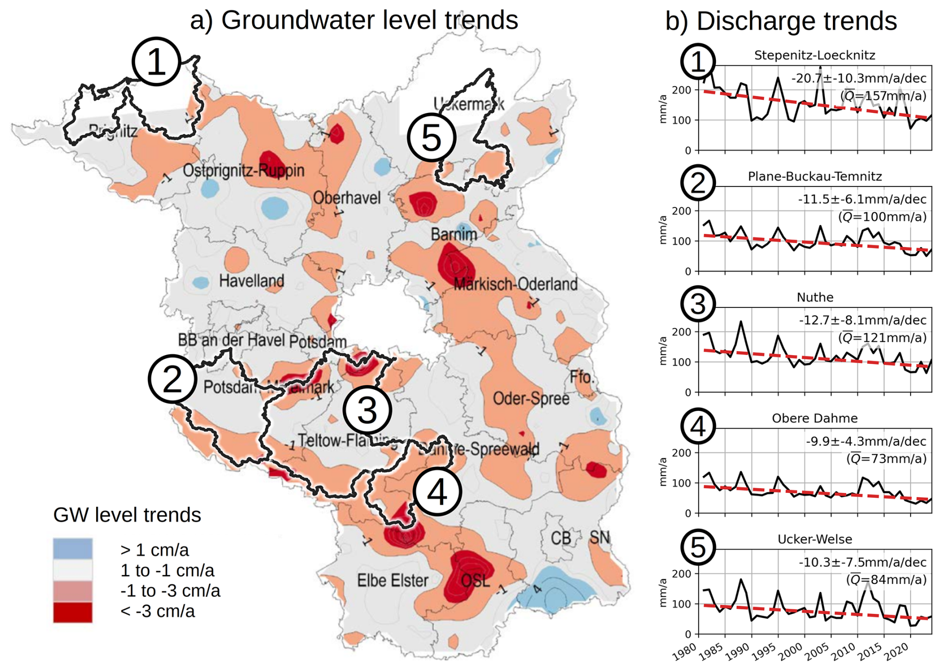
Figure 1 (a) Interpolated trends of groundwater levels from linear regression at groundwater gauges in Brandenburg from 1976 to 2020, figure modified from Landesamt für Umwelt Brandenburg (2022) (text in the map refers to county names); (b) Theil–Sen trends (all highly significant) of observed discharge (from 1980 to 2022) at selected river and stream gauges in Brandenburg that are largely unaffected by direct anthropogenic interference (see Sect. 2.2 for details on the underlying data); the unit of the trends (mm a⁻¹ per decade) correspond to the change in discharge (in mm a⁻¹) per time period, i.e. decade (dec).

First, groundwater levels decreased significantly between 1976 and 2020 in the recharge areas (i.e. in the elevated areas with large distances to the groundwater table; see Fig. 1). The most plausible hypothesis to explain such a state-wide prevalence of negative trends is a declining GWR, while there is no evidence for any widespread increase in groundwater abstractions in the past decades. Quite the contrary, water abstractions have considerably decreased, at least since 1991 (Landesamt für Umwelt Brandenburg, 2022). Concerning the groundwater levels, it has to be noted that the lowlands do not show strong trends in either direction because the groundwater level is stabilized by the water level of the heavily regulated streams and rivers to which the aquifers are connected.

Second, the discharge of many rivers in Brandenburg has been significantly decreasing since 1980. Figure 1 shows discharge observations for five river basins (or combinations of such; see Sect. 2.2 for details) that can be considered largely unaffected by anthropogenic influences such as inter-basin water transfers or open-pit mining (which widely occurs in the catchments of the rivers Spree and the Schwarze Elster and involves, in the active phase, pumping of groundwater into rivers and, in the restoration phase, the flooding of abandoned mining pits from groundwater or surface water, which may dominate groundwater and discharge dynamics; see Kröcher et al., 2025). The discharge series shown in Fig. 1 represent river basins with continuous discharge records since at least 1980 and with upstream catchment areas of at least 500 km², which allows us to assume some level of representativeness for the regional water balance and reduces the sensitivity to uncertainties in belowground catchment areas. According to these records, the decrease in discharge since 1980 is highly significant, corresponding to a rate between −21 and −10 mm a⁻¹ per decade and a total loss of around 40 % since 1980. Given the highly permeable soils in Brandenburg and the resulting insignificance of surface runoff (LUA Brandenburg, 2001), the discharge of these catchments can be considered to be almost exclusively fed from groundwater recharge; any long-term decrease in discharge must hence be caused by a declining GWR, given the absence of other dominant processes of anthropogenic interference, as mentioned above.

Certainly, GWR is an elusive variable that is difficult to quantify and impossible to measure directly at the landscape scale. Interestingly, the aforementioned evidence for a decreasing GWR in Brandenburg is in contrast to a recently published modelling study (Umweltbundesamt, 2024) that reports, for large parts of Brandenburg, only minor and mostly insignificant changes in GWR in the past decades (while Marx et al., 2024, even project increasing GWR in the future). In this context, our study aims to identify potential reasons behind such inconsistencies or, in other words, to better understand which factors govern simulated GWR trends in Brandenburg over the past decades and could hence explain the observed discharge trends.

For this purpose, we set up a range of simulation experiments to model GWR from 1980 until 2023 for the five aforementioned river basins in Brandenburg, and we compare the corresponding simulated trends to observed discharge trends in these basins. To that end, we use a combination of model and data that is specifically tailored to the conditions in Brandenburg. In the following, we highlight specific aspects of this setup and some of the underlying assumptions (details with regard to data and modelling will be described in Sects. 2 and 3, respectively):

• Long-term trends in discharge are governed by GWR. As already elaborated above, large parts of Brandenburg are dominated by permeable sandy soils. Hence, surface runoff is negligible (LUA Brandenburg, 2001), and river discharge is mainly fed from groundwater exfiltration. Any long-term trend in discharge can thus be interpreted as a long-term trend in GWR. The emphasis is on long-term, in the sense of multiple decades, since we can assume that over long time periods, any GWR will also end up in the surface waterbodies that drain the system. Short-term dynamics of river discharge (e.g. across rainfall events or seasons) are, however, governed by the travel times of water along the different transit paths in the vadose zone and the aquifer. In contrast to discharge records, it is difficult to quantitatively infer representative GWR trends from time series of groundwater levels because of the uncertainty in the storage coefficient, the uncertain contribution of the upstream area to the observed level dynamics, the potential effects of local groundwater abstractions, and the limited spatial coverage of observation points. Consequently, understanding of groundwater recharge dynamics from groundwater-level data is hampered by inconsistent patterns, e.g. opposing trends (Lischeid et al., 2021).

• The distance of the soil surface to the groundwater table is of utmost importance. On the one hand, shallow groundwater tables in the lowland areas lead to very high evapotranspiration and hence to water budgets that are fundamentally different from areas with a deep groundwater table (LUA Brandenburg, 2001). The reason for this is the strong connectivity of the vegetation's root system to the groundwater table. On the other hand, a deep groundwater table (in Brandenburg up to more than 50 m) implies long transit times for the infiltrated water to reach the aquifer. Given the possibility of transit times on the order of years to decades, any change in the soil water balance might propagate quite slowly to the groundwater table. In order to capture all relevant processes across the entire unsaturated zone and range of transit times, we apply a physically based one-dimensional soil hydraulic model (the Soil-Water-Atmosphere-Plant (SWAP) model; van Dam et al., 2008) in which we conceive annual GWR as the net amount of percolation water that actually reaches the groundwater table after passing the entire unsaturated zone. Given the potentially long transit times of up to decades, our simulation already starts in 1951, even if we evaluate simulated GWR only from 1980 to 2023.

• Long and homogeneous observational records of hydro-climatic variables are required in order to identify potential long-term trends in GWR. In this context, it should be emphasized that climate change is not limited to global warming (i.e. a temperature rise) but that other relevant climate variables might be subject to long-term trends, such as increasing solar irradiation (“global brightening”, e.g. Wild, 2009), decreasing wind speed (“terrestrial stilling”, e.g. Vautard et al., 2010), or trends in precipitation (in any direction). Unfortunately, the two criteria of “record length” and “homogeneity” can be considered antagonistic in some instances: with the HYRAS dataset (Razafimaharo et al., 2020), the German Meteorological Service (Deutscher Wetterdienst, DWD hereafter) indeed provides a long record of daily grids of important hydro-climatic variables from 1951 until 2020, based on interpolated gauge measurements. However, the underlying set of observational gauges can vary substantially over time so that “trends in any one area may reflect the appearance and disappearance of specific stations, rather than the true local trend” (quoted from Hofstra et al., 2010). In our study, we hence decided to only use long-term observations from single climate stations instead of HYRAS data (exceptions are documented in Sect. 3.5) – being aware, of course, that these could be subject to inhomogeneities, too (e.g. due to changes in instruments, in measurement locations, or in the surroundings of the measurement locations; Peterson et al., 1998). Only very few climate stations remain in Brandenburg which provide long daily records of the required climate variables (temperature, relative humidity, and precipitation being the most complete, sun hours and wind speed being more problematic). In fact, we reduced our analysis to four climate stations (Potsdam, Lindenberg, Angermünde, Marnitz) with the most complete records between 1951 and 2023 and with the greatest proximity to our five study catchments. Only for precipitation did we extend this approach (further details with regard to the construction of homogeneous climate forcing data for our simulation model are provided in Sect. 3.2).

• The leaf area index (LAI) is a key vegetation parameter with potentially transient behaviour. The LAI affects both transpiration and interception losses and has hence a fundamental impact on the actual evapotranspiration and, consequently, groundwater recharge. At the same time, there is strong evidence from remote sensing that the LAI has, in many regions of the world, significantly increased since the 1980s (“Earth's greening”; Yang et al., 2023). In our study, we use a recently published LAI dataset (Cao et al., 2023) which spans 1982 to 2020 in order to analyse the prevalence of such an LAI trend in Brandenburg as well as the potential effect on GWR trends.

In Sects. 2 and 3, we will give an overview of the data (namely discharge records, climatological data, landscape, and vegetation attributes) and methods (namely the filling of gaps in climatological data, the soil hydraulic model, and the design of our simulation experiments). In Sect. 4, we will present the GWR trends and their significance as resulting from our simulations and discuss how these trends compare to the observed discharge trends. In Sect. 5, we will comprehensively discuss limitations and uncertainties of our approach and perspectives to address these in prospective research. In Sect. 6, we highlight the implications of our study for both research and water resource management.

2 Data

2.1 Study area

Figure 2 gives an overview of the study area and some of the underlying data. Brandenburg has a temperate continental climate characterized by cold winters and warm summers and moderate precipitation that is evenly distributed throughout the year (mostly Cfb climate according to the classification of Köppen and Geiger). Conditions are slightly drier in the east, while maximum precipitation depths occur in the northwest and in the south (see also Fig. 2).

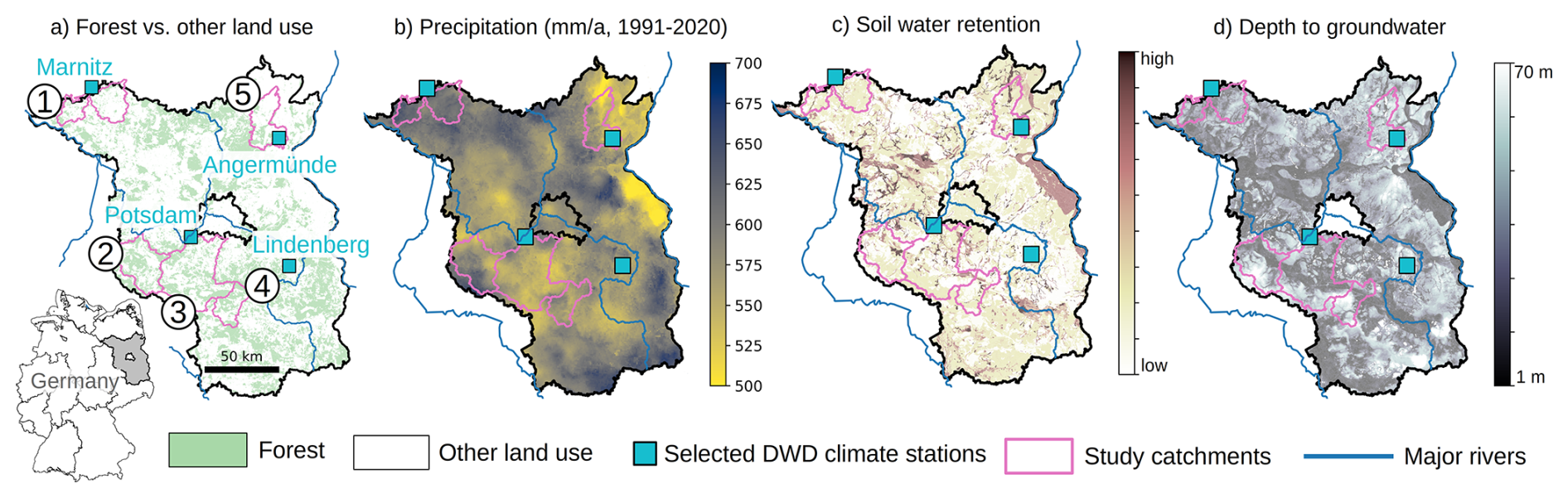
Figure 2 Overview of study catchments, selected DWD climate stations, and the spatial distribution of selected climate and landscape attributes: (a) land use (forest versus other land use (i.e. mainly grassland/cropland, © OpenStreetMap contributors, 2024, distribution under ODbL license); (b) average annual precipitation sum for the climate-normal period, 1991–2020, based on DWD's HYRAS-DE-PR; (c) top soil water retention capacity (LBGR, 2024); and (d) depth to the groundwater table (LfU, 2013).

The vast lowland areas of Brandenburg (mostly Urstromtäler from the Weichsel glacial period) are dominated by shallow groundwater tables and hence high evapotranspiration rates, typically leading to a net water loss from these areas. Recharge of the groundwater mainly takes place in the more elevated areas, mostly consisting of moraines from the Weichsel epoch, except the south and west, which are dominated by the Saale epoch. Soils are dominated by highly permeable sandy soils and loamy sands, as well as organic soils in the lowlands (LBGR, 2024).

The land use in Brandenburg is composed of 47.6 % agriculture, 35.0 % forests, 3.6 % other vegetated areas, 6.7 % settlements, 3.5 % traffic infrastructure, and 3.5 % surface waters (Amt für Statistik Berlin-Brandenburg, 2023).

2.2 Discharge records

As river discharge in Brandenburg is governed by groundwater fluxes, we use long-term discharge observations as a reference for long-term changes in groundwater recharge (see Sect. 1). Daily discharge observations are provided by the Brandenburg state environmental agency (Landesamt für Umwelt, referred to as LfU hereafter) via an online platform (Landesamt für Umwelt, 2025).

Table 1 Overview of selected discharge gauges in Brandenburg and of combinations of catchments; trends are only computed for catchments or combinations larger than 500 km².

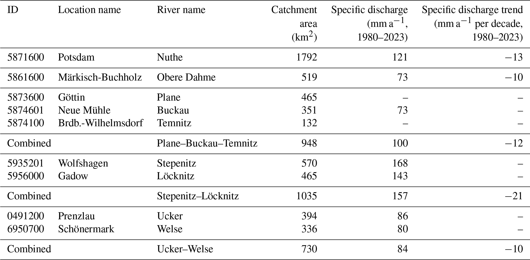
The following criteria were applied to select discharge gauges for our analysis (see also Sect. 1): (1) discharge records from at least 1980 to 2023; (2) a minimum upstream area of 500 km² to reduce the effect of uncertainties in the delineation of belowground watersheds; and (3) no major anthropogenic manipulation of the catchments' water balance, e.g. by inter-basin water transfers or open-pit mining (see Sect. 1). In three cases, adjacent catchments were aggregated in order to further reduce the effect of uncertain belowground watersheds and to increase the area over which the water balance is computed. “Aggregating” two (or three) catchments means that their areas were merged into one coherent area and that the observed runoff at the gauges of each catchment was summed in order to obtain the total runoff from the merged area. Table 1 gives a comprehensive overview of the discharge gauges used and the aggregation of catchment areas and runoff gauge observations for our analysis.

2.3 Climate observations

Except for precipitation (see Sect. 2.4), the hydro-climatological model forcing is entirely based on the climate station records (DWD, 2024a) provided by the German Weather Service (Deutscher Wetterdienst, DWD hereafter). Since the homogeneity of the forcing data is essential when analysing long-term GWR trends, we did not use gridded products (such as HYRAS-DE) which are based on interpolation (Hofstra et al., 2010, and also Sect. 1 for more explanation).

Instead, we identified four DWD climate stations in Brandenburg that (1) are close to the selected study catchments and (2) show a fairly complete record of required daily climate variables over the time period from 1951 until 2023: Potsdam, Lindenberg, Angermünde, and Marnitz. These stations are highlighted in Fig. 2. The climate variables required from these stations include daily solar irradiance (kJ m⁻² d⁻¹), precipitation (mm d⁻¹), daily minimum and maximum temperature (°C), relative humidity (%), wind speed (m s⁻¹), and daily sunshine hours (h d⁻¹, required in case solar irradiance is unavailable; see Sect. 3.2).

Still, not all required climate variables were recorded at all stations, and some stations still exhibit data gaps. In Sect. 3.2, we document how we filled the data gaps for different climate variables and stations while attempting to maintain homogeneity of the time series as best as possible.

2.4 Precipitation observations

Long-term precipitation trends are much less coherent across Brandenburg compared to trends for other climate variables. In addition, more precipitation stations exist than climate stations. Therefore we decided to evaluate the effect of different precipitation forcings on the trends of simulated GWR. For that purpose, we included the following precipitation times series in addition to those observed at the four climate stations.

• We included observations from other precipitation gauges (DWD, 2024b) within a 5 km buffer around each study catchment. Since there is a trade-off between the number of available station records versus the length and completeness and hence the homogeneity of these records, we decided to apply the following filtering criteria: we used only stations with less than a total of 1 % missing data between 1980 and 2023 and less than 5 % missing data for individual years between 1980 and 2023. We also included gauges with records that do not fully reach back until 1951. These will be specifically marked in the results since the corresponding GWR simulation will not have a fully homogeneous forcing during model spin-up. Based on these criteria, we obtained between 0 and 7 additional precipitation records for each study catchment (see Table 3).

• We already pointed out that using gridded hydrometeorological interpolation products is prone to introducing artificial local trends, specifically in a setting in which many precipitation gauges were introduced between 1960 and 1980 but discontinued after 1990. Still, we investigate the effect of one such product (HYRAS-DE-PR; DWD, 2024c), simply because this is the most prominent regionalized precipitation product for climate impact studies in Germany. For that purpose, we use the daily areal average of HYRAS-DE-PR across the selected study catchments from 1951 to 2023.

2.5 Leaf area index and other vegetation parameters

In order to correctly capture the magnitude and seasonality of forest LAI, we used data from Level II plot collections of the UNECE Convention on Long-range Transboundary Air Pollution (ICP Forests), which comprise eight forest sites for Brandenburg, five of which monitor Scots pine (Pinus sylvestris) forests which represent 70 % of the state's forests. The data on these five sites reach back to 2016. On this basis, we constructed the average seasonal LAI development for this species. A similar procedure was applied to construct the average seasonal progression of LAI for grassland and cropland, based on typical crop representations for Central Europe in the SWAP model library (Kroes et al., 2017).

In order to quantify and consider potential long-term trends in LAI, we used a dataset of global LAI estimates from 1982 to 2020 that was recently published by Cao et al. (2023). The aim of this dataset is specifically to maximize spatio-temporal consistency. For this purpose, various satellite-based normalized difference vegetation index (NDVI) and LAI products as well as millions of field LAI measurements were fused by means of a back propagation neural network. The spatio-temporal resolution of the dataset is $\mathrm{1}/\mathrm{12}$° (about 5 km in Brandenburg) and approximately 2 weeks. For our study, we extracted the data for Brandenburg and computed, for each time step, the areal average LAI for the entire state (in order to get a more robust signal in comparison to computing areal average values only for the selected catchments). For the resulting time series of biweekly LAI values from 1982 to 2020, we computed a Theil–Sen trend which amounted to an increase of 0.1 m² m⁻² per decade. This trend was superimposed on the aforementioned seasonal LAI developments for forest and grassland in the SWAP model (see also Sect. 3.4, and Sect. 5.3 for a discussion on the limitations of this approach).

2.6 Other geodata

In order to categorize the landscape, within each considered river basin, into similar functional units (hydrotopes), we used the following data sources for land use, soil, and the distance to the groundwater table:

• Land use. To delineate forests from grassland and cropland, we used the land use layer from OpenStreetMap (OpenStreetMap contributors, 2024).

• Soil data. We used the BUEK300 soil map (LBGR, 2024) in order to obtain the dominant soil type per study catchment (medium sand for all catchments except Ucker–Welse and Stepenitz–Löcknitz, for which the dominant soil is loamy sand) and the corresponding dominant soil texture, which is required as an input to a pedotransfer function to determine the soil hydraulic parameters of the simulation model (see Sect. 3.4).

• Depth to the groundwater table. To represent the depth of the groundwater table and hence the lower boundary condition for the soil hydraulic model, we used a dataset provided by the Brandenburg Landesamt für Umwelt (LfU, environmental state agency) which represents the depth of the unsaturated zone as obtained from a combination of a digital elevation model and groundwater-level contours constructed by means of interpolation (LfU, 2013). The dataset provides the midpoints of depth classes, corresponding to a finite number of 13 depth classes (1, 2, 3, 4, 5, 7.5, 10, 15, 20, 30, 40, 50, and 70 m). The depth resolution is higher (metre resolution) for shallow groundwater tables, which is particularly important for modelling the water balance (Sect. 3.4), since the groundwater depth has a strong influence on evapotranspiration when the groundwater table is shallow (see Sect. 1).

3 Methods

3.1 Methodological overview

The main methodological approach of our study is to simulate series of GWR in each study catchment for the period from 1980 to 2023. From these series, we computed the trends in GWR and compared them to the corresponding trends of observed discharge. Good agreement between both would indicate that the simulation model is able to explain the discharge trends as outlined in Fig. 1 and Table 1 (see also Sect. 1 for additional background).

To obtain GWR, the one-dimensional Soil-Water-Atmosphere-Plant (SWAP) model (van Dam et al., 2008, Sect. 3.4) was used to simulate the surface water balance and the resulting percolation of water through the unsaturated zone down to the groundwater table. This daily “bottom flux” was aggregated to obtain the annual sum of groundwater recharge.

In order to obtain the spatial average of GWR per catchment, we followed the concept of “hydrotopes”, i.e. spatial sub-units that are considered homogeneous with regard to (i) climate forcing, (ii) soil texture, (iii) land use, and (iv) groundwater depth. For each catchment, climate and soil were assumed to be uniform across the entire catchment (i.e. one class each per catchment): the climate forcing was based on the nearest of the four selected climate stations (Sect. 2.3), and soil texture was represented by the dominant soil texture class in the catchment (Sect. 2.6). Land use and groundwater depth, however, were assumed to be heterogeneous across the catchment: land use was represented by 2 classes (forest and grassland/cropland) and groundwater depth by 13 classes (see Sect. 2.6). This resulted in a total of 26 hydrotope classes (1 climate × 1 soil × 2 land uses × 13 groundwater depths). By spatially intersecting all four layers, we quantified the areal fraction of each hydrotope class per catchment. Running the SWAP model for each of the 26 hydrotope classes, the daily GWR per catchment was then obtained as the area-weighted average of the simulated daily bottom flux per hydrotope.

In the following subsections, we further explain the treatment of missing hydro-climatological data (Sect. 3.2), the precipitation correction (Sect. 3.3), the SWAP model and its parameterization (Sect. 3.4), the specific design of the simulation experiments (Sect. 3.5) and the calculation of trends (Sect. 3.6).

3.2 Filling missing data for solar irradiation and wind speed

For Potsdam, Lindenberg, Angermünde, and Marnitz, the percentage of missing data between 1951 and 2023 is below 0.1 % for each of the following variables: daily minimum/maximum temperature, relative humidity, and precipitation depth. For solar irradiation and wind speed, though, only Potsdam has an almost complete record (less than 1 % missing data). Records of solar irradiation in Lindenberg only started in 1980 and have considerable gaps between 1997 and 2001 (while wind speed at Lindenberg has less than 1 % missing data). Angermünde and Marnitz have no records of solar irradiation, and measurements of wind speed only started around 1980. Furthermore, many wind speed measurements across Brandenburg are affected by strong inhomogeneities, mainly because the measurement height varied over time. In the following, we outline our approach to provide fairly homogeneous time series for solar irradiation and wind speed as our model forcing.

Solar irradiance is a key input to the computation of evapotranspiration using the Penman–Monteith method; however, Potsdam is the only climate station in the state with a comprehensive record from 1951 to 2023. Lindenberg, in turn, has an almost complete record of daily sunshine hours. Using the observations of solar irradiance and sunshine hours in Potsdam, we trained a random forest (100 trees and a maximum node depth of 10) to model solar irradiance from the following predictive features: clear-sky radiation as simulated from geographic coordinates, altitude, and date–time by the Python package pvlib (Holmgren et al., 2018; Anderson et al., 2024; using the function “get_clearsky” and aggregating from 20 min resolution to daily sums of radiation), sunshine hours per day, relative and absolute humidity, and seconds elapsed since 1951. The resulting random forest model yielded an R² of 98.4 % on independent test data, with clear-sky radiation and sunshine hours being the most important features by far. We used this random forest model to fill the data gaps for solar irradiance at Lindenberg. For the climate stations in Angermünde and Marnitz, however, the record of sunshine hours between 1951 and 2023 had too many gaps. In order to ensure a homogeneous record of sunshine hours as an input to the random forest, we used the sunshine data from Potsdam and applied a multiplicative scaling factor to adapt it to the average conditions in Angermünde and Marnitz. This factor was obtained from the ratio of the mean values at both stations (Potsdam and Angermünde or Marnitz, respectively) for those periods in which both stations had data. With these complete records of sunshine hours, the aforementioned random forest model was applied to Angermünde and Marnitz in order to obtain solar irradiance.

Wind speed is observed at 23 DWD stations in Brandenburg. At only seven of these does the sensor measure at 10 m above ground – a reference height commonly used in precipitation correction and for calculating evapotranspiration. With record lengths of 10–52 years, none of these stations covered the entire study period (1951–2023). Conversely, ERA5-Land (Muñoz Sabater et al., 2021) offers hourly values for wind speed at approximately 9 km resolution. However, ERA5-Land only showed poor agreement with observed trends and magnitudes. In order to obtain continuous wind speed records at the seven aforementioned stations, we trained a random forest model (100 trees, maximum node depth of 10) at each of these stations using the available daily wind speed observations at 10 m as training data. As predictive features, we used the local daily ERA5-Land wind speed estimates and the wind speed observed at the climate station in Potsdam. R² values ranged from 0.74–0.89 on independent test data. These random forest models served for reconstructing daily wind speed at the seven stations for the full study period. For Potsdam, Lindenberg, Angermünde, and Marnitz, we then used the reconstructed wind speed at the nearest of these seven wind stations.

3.3 Precipitation correction

Standard precipitation gauges experience considerable undercatch, mainly due to wind-induced turbulence. To account for the effects on rain and snow, we used the correction according to Kochendorfer et al. (2017) for unshielded gauges, which requires wind speed at 10 m (see Sect. 3.2) and air temperature at 2 m. It should be emphasized that this correction method could affect the trend of the corrected precipitation in cases where the underlying wind speed records show a trend. This is, however, an intended behaviour because a change in wind speed at the gauge location also changes the corresponding measurement error that needs to be corrected for. To assess this effect, we also analysed the uncorrected precipitation and the standard correction used by DWD (Richter, 1995), which uses fixed monthly coefficients for geographic regions and station exposure (codes C and d, according to Richter, 1995).

3.4 Soil hydraulic model

The Soil-Water-Atmosphere-Plant (SWAP; van Dam et al., 2008) model was employed to simulate soil water dynamics and groundwater recharge within the study area. This 1D model calculates vertical soil water movement by solving the Richards equation, which accounts for infiltration and capillary rise, based on soil hydraulic properties and governing boundary conditions. Evapotranspiration depends on atmospheric conditions as well as on vegetation and soil properties and is estimated using the Penman–Monteith equation in combination with the Feddes model, which accounts for the limitation of transpiration by the availability of soil water (Kroes et al., 2017). The dual focus on soil hydrology and atmospheric interactions allows for a detailed analysis of the surface water balance and the percolation of water through the unsaturated zone down to the groundwater table. This “bottom flux” is considered the groundwater recharge (which can also be negative in the case of a net flux from the groundwater table to the surface, typically in the case of areas with shallow groundwater tables during the summer). For our model setup, the groundwater table depth was considered static (corresponding to a Dirichlet boundary condition; see also Sect. 2.6).

Guerrero-Ramírez et al. (2021)Guan and Wilson (2009)Von Hoyningen-Huene (1983)Kroes et al. (2017)Gash et al. (1995)Russ et al. (2016)

Table 2 Overview of key SWAP model parameters related to vegetation and corresponding references.

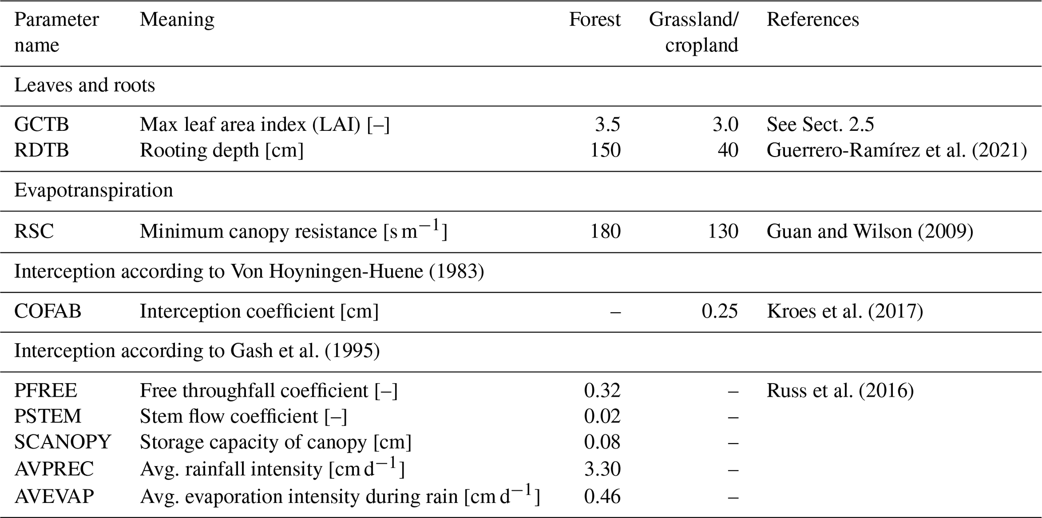
Table 2 highlights important vegetation-related model parameters that were used for our study. Furthermore, soil hydraulic parameters (SHPs) need to be set in order to represent the relationships between matric potential (ψ, hPa) and volumetric soil water content (SWC, m³ m⁻³) as well as hydraulic conductivity (m d⁻¹). Using the model of van Genuchten and Mualem (van Genuchten, 1980), the SHPs correspond to five parameters: residual water content (θ_r, m³ m⁻³), saturated water content (θ_s, m³ m⁻³), the air entry point (α, m⁻¹), the shape parameter of the retention curve (n, dimensionless), and the saturated hydraulic conductivity (K_s, m d⁻¹). The values of these parameters were set based on the widely used pedotransfer function ROSETTA (Schaap et al., 2001), which requires soil texture and soil bulk density as input. These soil parameters were obtained from the soil map BUEK300 for the dominant soil in each study catchment (see also Sect. 2.6). Altdorff et al. (2024) have recently shown that the same model implementation and parameterization could reproduce soil water dynamics well across eight monitoring locations in Brandenburg (covering major land use and soil types as well as different groundwater table depths).

3.5 Design of simulation experiments

The hydro-climatic model forcing includes daily values for solar irradiation, temperature, humidity, wind speed, and precipitation. Except for precipitation, this forcing was obtained for each study catchment by assigning the observations (or reconstructed observations; see Sect. 3.2) of one of the four selected climate stations (see Table 3). Due to the importance of precipitation for GWR and the large uncertainty in precipitation trends (due to high interannual variability), we tested a larger set of precipitation time series as model forcing for each study catchment:

• the precipitation observed at the selected climate station;

• synthetic trends, removing the trend from the observed precipitation at the selected climate station and then imprinting different linear trends, ranging from −20 to +20 mm a⁻¹ per decade in increments of 2 mm a⁻¹ per decade;

• precipitation observed at other precipitation gauges (individually, i.e. without any further weighting) in or close to the study catchments (refer to Sect. 2.4);

• the areal average of precipitation in the study catchment as obtained from the gridded HYRAS-DE-PR dataset (refer to Sect. 2.4).

Table 3 Overview of simulation experiments and input data used. The last column explains the number of resulting realizations as the product of the number of precipitation variants (third column) and the number of LAI input variants (fourth column).

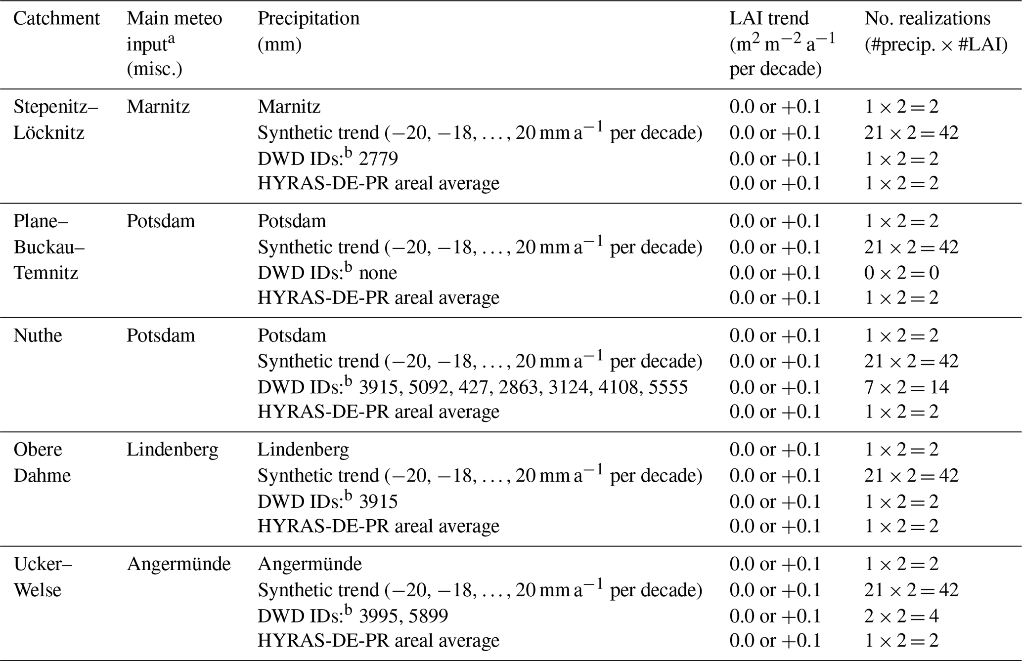
^a Daily minimum and maximum air temperature at 2 m, relative humidity at 2 m, solar irradiation, and wind speed at 10 m. ^b IDs of DWD's precipitation gauges which were used as alternative precipitation forcing (see Sect. 3.5).

In combination with the two LAI scenarios (static versus transient), this resulted in a total number of 262 realizations (see Table 3).

3.6 Trend calculation

All trends in this paper were calculated using Theil–Sen estimates (Theil, 1992; Sen, 1968) to compute the slope of the trend. This method is commonly used in hydrometeorological analyses (see, for example, Yue et al., 2002) and is more robust to outliers and independent of the assumption of normally distributed residuals, while otherwise producing results similar to linear regression. All trends are reported with reference to a 10-year period​​​​​​​. The significance of the trends is likewise computed according to Sen (1968) and expressed as the p value.

4 Results and discussion

4.1 Trends in hydro-climatic model forcing

Figure 3 summarizes the hydro-climatological model forcing at the four selected DWD climate stations in Brandenburg: Potsdam, Lindenberg, Marnitz, and Angermünde. The potential evapotranspiration (ET_P, computed using the Penman–Monteith method according to Kroes et al., 2017) shows a highly significant positive trend across all four stations (similar for all stations but highest at Lindenberg). ET_P integrates the effects of other climate variables, namely solar irradiation and air temperature, which increase at all stations (causing the effective increase in ET_P), and wind speed, which decreases at all stations (counteracting the increase in ET_P).

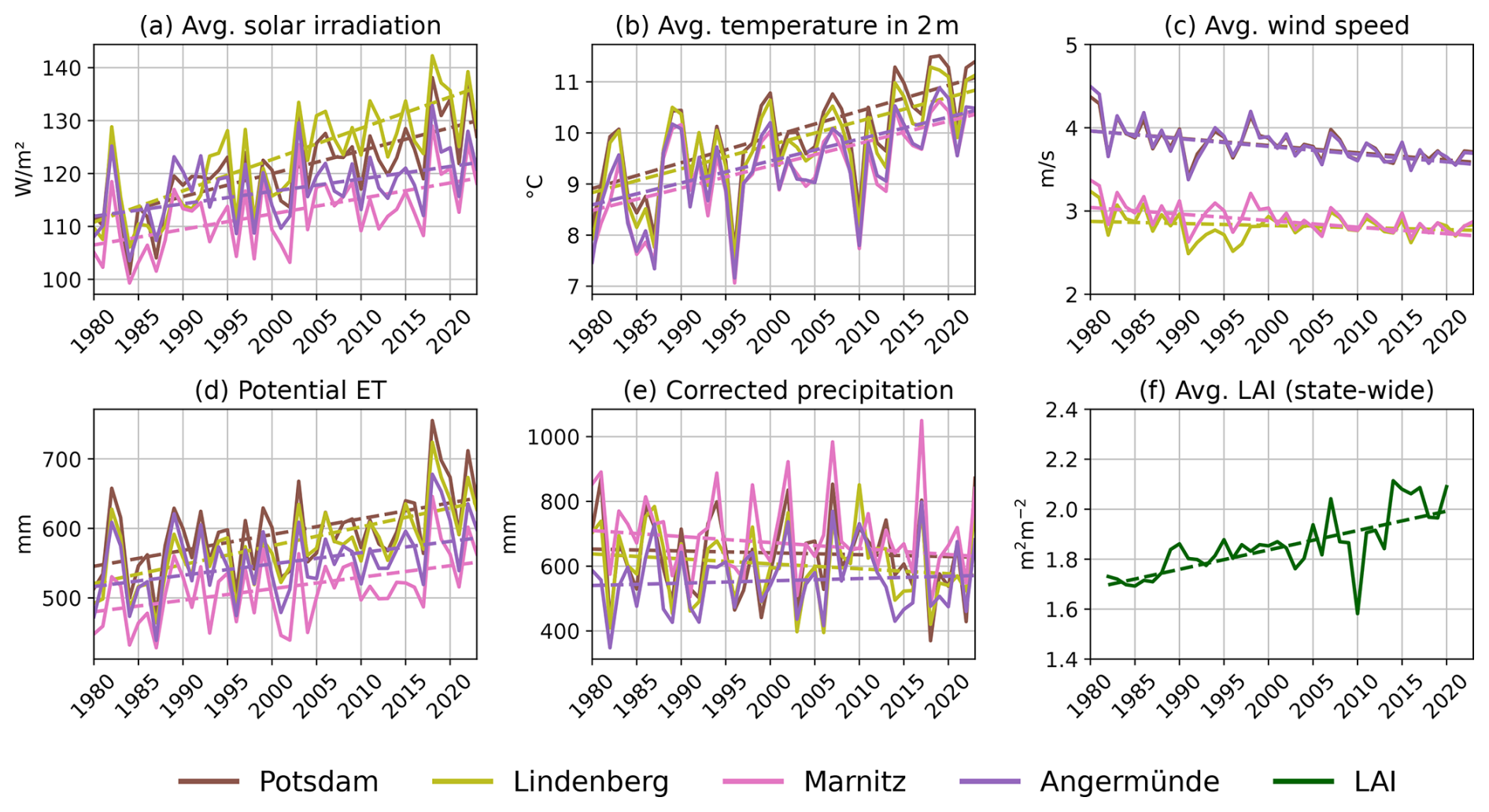
Figure 3 Aggregate annual values of selected climate variables at DWD's climate stations Potsdam, Lindenberg, Marnitz, and Angermünde from 1980 to 2023 and LAI as obtained from Cao et al. (2023) (only available from 1982 to 2020): (a) solar irradiation (annual average), (b) air temperature at 2 m (annual average), (c) wind speed (annual average), (d) reference evapotranspiration (annual sum), (e) precipitation (corrected according to Kochendorfer et al., 2017, annual sum), and (f) Brandenburg-wide average LAI (annual average). Dashed lines show Theil–Sen trend slopes, which are all highly significant except for precipitation, for which none of the trends is significant; note that series for solar irradiation and wind speed were partly reconstructed (see Sect. 3.2) and potential ET was computed using the SWAP model.

While it is obvious that any trend in ET_P will not directly translate into actual evapotranspiration (which is constrained by actual soil water availability), ET_P represents a forcing component that consistently acts towards an increase in actual evapotranspiration and hence a decrease in GWR across all stations.

As for precipitation, the four climate stations feature negative trends at Potsdam, Lindenberg, and Marnitz (all at similar rates), and a positive trend at Angermünde. However, none of these trends is significant. The situation is similar if we include other precipitation gauges in Brandenburg (Fig. 4): looking only at gauges with complete records, opposite trend directions exist across the state between 1980 and 2023, ranging roughly between −20 and +20 mm a⁻¹ per decade.

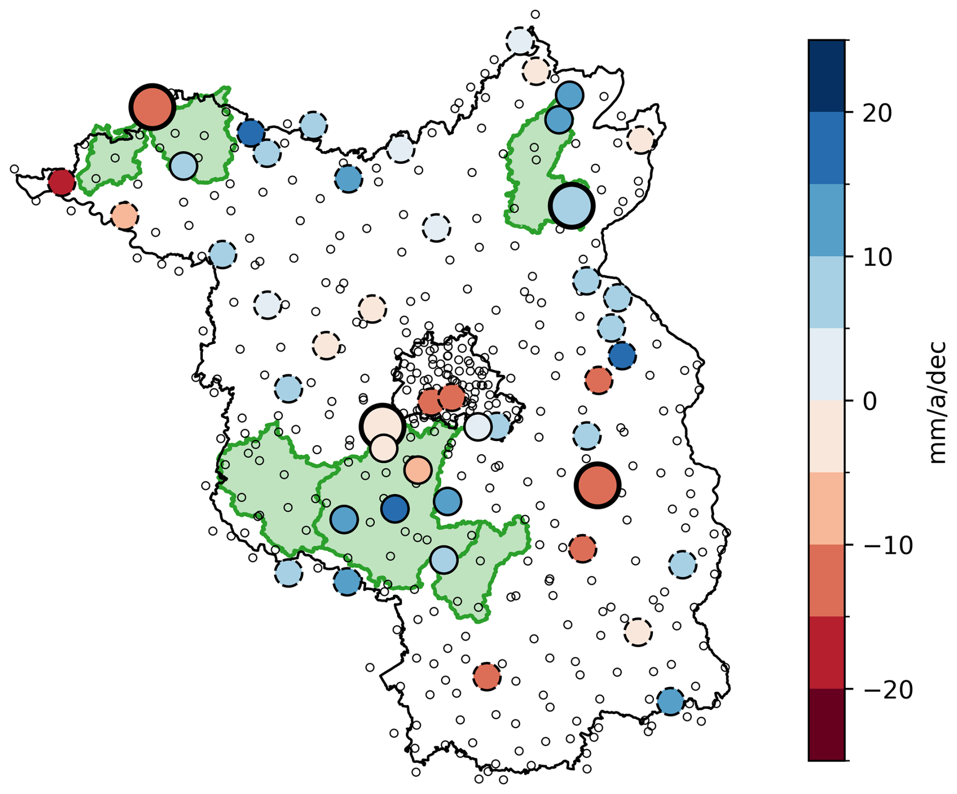
Figure 4 Precipitation trends between 1980 and 2023: the small unfilled dots show all daily precipitation gauge locations in DWD's collection; the coloured dots show the trend at gauge locations with complete records at least between 1980 and 2023 (large dots: trend at the four selected climate stations Potsdam, Lindenberg, Marnitz, and Angermünde; dots with solid outlines: precipitation gauges within the catchments – see Table 3; dots with dashed outlines: other gauges with complete records). Note that none of the shown trends is significant at the 5 % level.

Precipitation correction (see Sect. 3.3) not only corrects the total amount (i.e. +4–6 mm a⁻¹ for Kochendorfer et al., 2017, +9–10 mm a⁻¹ for Richter, 1995), but also may affect the trends: Kochendorfer et al. (2017) reinforce the negative trends by up to −4 mm a⁻¹ per decade, while Richter (1995) shows a minor amplification of positive trends (results not shown).

Again, none of these trends is significant, but even insignificant precipitation trends might affect trends in simulated GWR. The simulation experiment covers various combinations of precipitation series for each catchment in order to investigate the relevance of this effect.

4.2 Trends in GWR

Figure 5 shows annual series of simulated GWR (solid blue lines). As examples from the simulations experiments in Table 3, we chose the ones in which the model was forced by the observations from the four selected climate stations (including precipitation), together with the specified LAI trend of 0.1 m² m⁻². In comparison to the annual series of observed river discharge (solid black lines), we find that the interannual variability and the average water balance match fairly well, with some overestimation in the Stepenitz–Löcknitz catchment and some underestimation in the Nuthe catchment. In general, the response of the river discharge is more dampened, which is plausible as it also includes the transit of water through the aquifer, which is not considered in our model. More importantly for our study, the long-term trends of observed discharge and simulated GWR correspond quite well – except for the Ucker–Welse catchment, where the modelled trend is much weaker than the observed one.

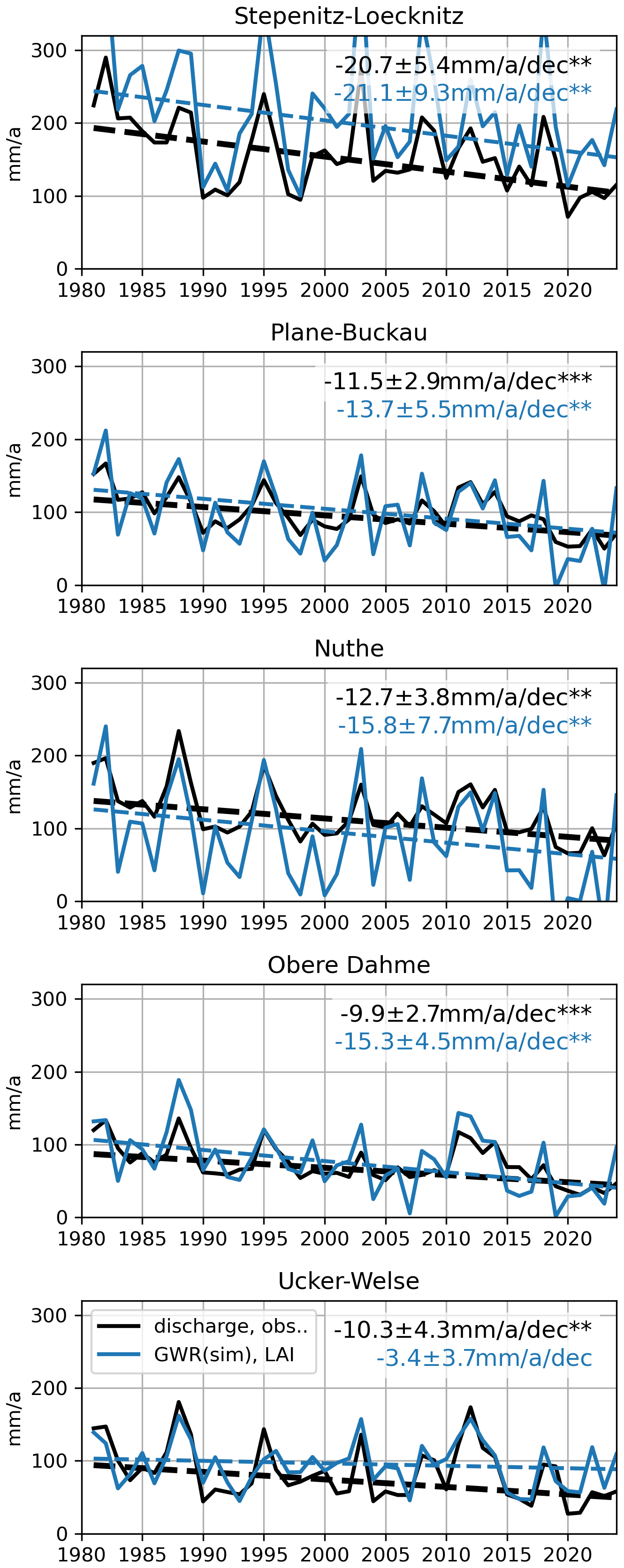
Figure 5 Annual observed river discharge and modelled groundwater recharge (1980–2023), driven by the selected climate stations, including the trend in LAI. The dashed lines illustrate the fitted trend; the (coloured) numbers specify the corresponding trend magnitudes, their 95 % confidence intervals, and the significance levels (${}^{\ast \ast \ast }$ p < 0.001; ${}^{\ast \ast }$ p < 0.05; ^∗ p < 0.1).

In order to put the trend examples from Fig. 5 into a more comprehensive context, Fig. 6 shows the simulated GWR trends as they result from all simulation experiments in Table 3.

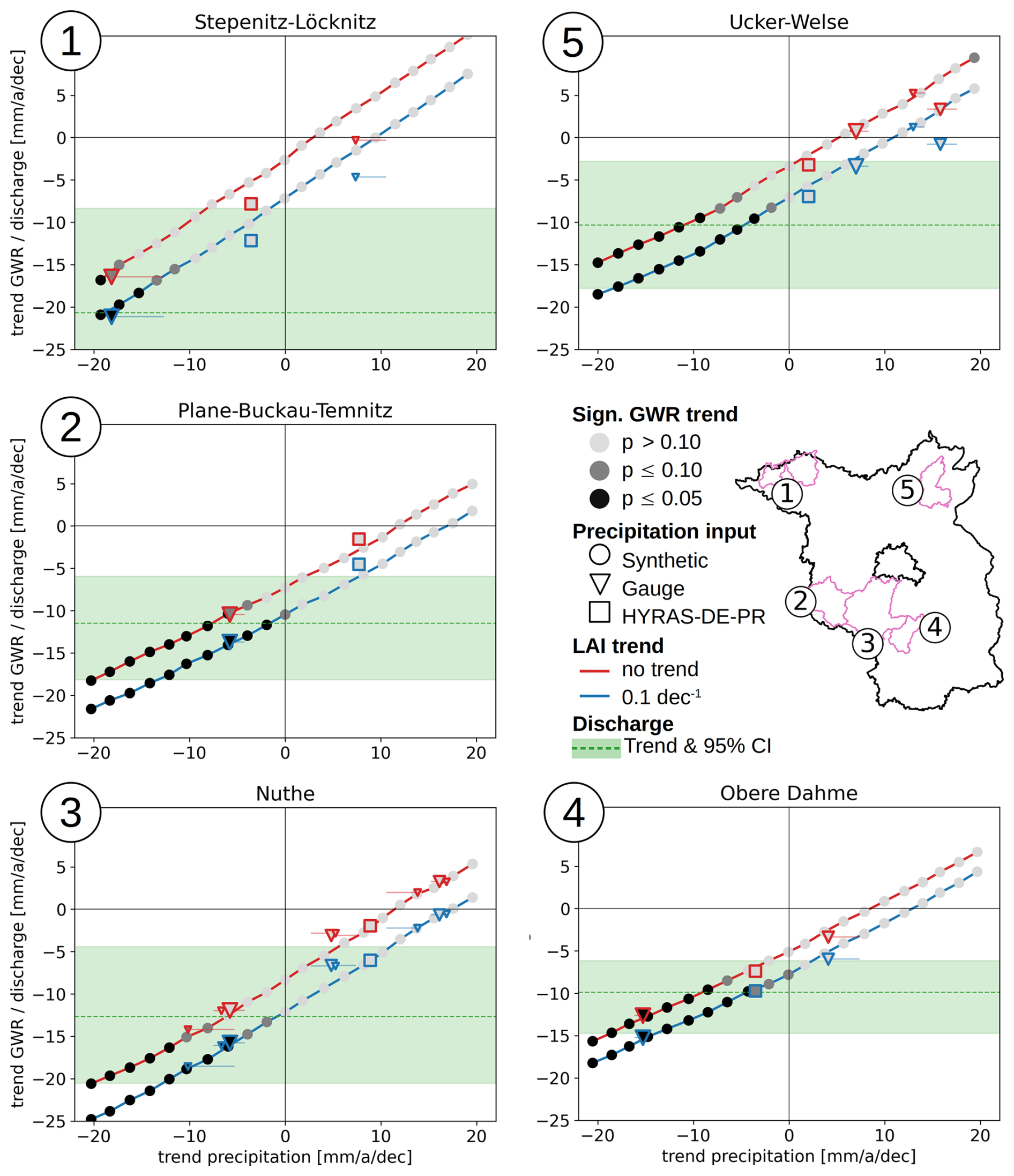
Figure 6 Effect of precipitation and LAI trends on GWR trends (1980–2023). Blue/red: with or without transient LAI trend; circles/lines: response to synthetic precipitation with superimposed trend; triangles: response to precipitation observed at selected gauges (large: selected climate station; medium/small: other rain gauges within catchment complete since 1951/1980), corrected according to Kochendorfer et al. (2017); associated whiskers display range of rainfall corrections (uncorrected; Richter, 1995; and Kochendorfer et al., 2017).

In each catchment, the model forcing is based on the observations of one of the four selected climate stations – except for the variables precipitation and LAI. As summarized in Table 3, each model run within a given catchment represents the combination of a specific LAI forcing (“static LAI” or “transient LAI”; see Fig. 3f) with one precipitation forcing (which in turn is characterized by a specific trend). Hence, each point in the figure marks the combination of an LAI trend (blue/red colour), a precipitation trend (abscissa), and the resulting GWR trend (ordinate). Precipitation time series were obtained from the selected climate stations (large triangles), from additional precipitation gauges within the catchments (small triangles), from the gridded HYRAS-DE-PR dataset (squares), and from artificial series with superimposed trends (dots and lines). The fill colour of the markers illustrates the significance level of the resulting GWR trend. The horizontal green line represents the mean and the green shade the 95 % confidence interval (CI) of the observed discharge trends for each catchment. In order to understand how to relate Fig. 6 to Fig. 5, just note that the large blue triangles in Fig. 6 represent the same GWR trends as the blue lines in Fig. 5.

Altogether, the figure should help us to disentangle the effects of precipitation and LAI trends on simulated GWR trends and to evaluate how well the simulated GWR trends correspond to the trends in observed discharge (which, in the long run, should correspond to the actual trends in GWR). Along these lines, Fig. 6 allows the following observations.

• Negative precipitation trends act towards negative GWR trends (and the same, of course, in the opposite direction). As such, this qualitative statement may appear self-evident. Yet, the strength of this relationship, together with the wide range of observed precipitation trends (even though not significant), was surprising to us.

• There is a substantial offset between the blue (“transient LAI”) and red (“static LAI”) markers on the order of −3 to −5 mm a⁻¹ per decade, meaning that the LAI trend causes GWR trends to be more negative (in comparison to using the same seasonal LAI dynamics each year). Given that the LAI trend of 0.1 m² m⁻² a⁻¹ per decade is highly significant and retrieved from observations, we consider the corresponding simulations (blue markers and lines) to be more representative of the situation in the selected catchments than the red markers and will hence focus the following discussion on the blue markers.

• Our key question is whether the observations of climate variables and LAI produce simulated GWR trends that are consistent with the trends in observed discharge; in other words, do the resulting GWR trends fall within the 95 % CI of the observed discharge trend (green shade) and are they significant? First, we take a look at our prime hydro-climatological forcing data – the selected climate stations: all large blue triangles fall within the 95 % CI and are significant (except for the Ucker–Welse catchment, where the GWR trend is not significant). This strongly supports the hypothesis that the past climate and LAI trends together explain the observed decline in discharge.

• The situation becomes less coherent if we use the precipitation from HYRAS-DE-PR instead: while the large blue squares fall into the green interval for all catchments except the Plane–Buckau–Temnitz catchment, the corresponding GWR trend is at least significant at a level of p=0.1 (corresponding to all dots in Fig. 6 except those with the lightest shade of grey) in only one out the five cases, i.e. for the Obere Dahme.

• Considering additional precipitation gauges from the catchment as alternative model forcing further complicates the picture: for the Stepenitz–Löcknitz catchment, the one additional gauge falls out of the 95 % CI; for the Plane–Buckau–Temnitz catchment, there is no additional gauge; for the Nuthe catchment, three out of seven additional gauges fall out of the 95 % CI; for the Obere Dahme catchment, the one additional gauge falls into the 95 % CI; and for the Ucker–Welse catchment, the two additional gauges fall out of the 95 % CI.

• In four cases, the GWR trend as inferred from HYRAS-DE-PR (squares) falls between the trends inferred from rain gauges (triangles). This is plausible. Still, trends from HYRAS-DE-PR need to be considered with care (as repeatedly mentioned before) because they are based on temporally varying sets of gauges – which could result in trend artefacts. This may apply in the Ucker–Welse catchment, where the trend in HYRAS-DE-PR precipitation is smaller than the trend of any of the shown rain gauges.

• The majority of blue markers with sufficiently long records (11 out of 14 triangles and squares) fall inside the 95 % CI of observed discharge trends; yet, there appears to be a general gap in the sense of simulated GWR trends underestimating the magnitude of the observed negative discharge trends or even being positive.

• It should be noted that none of the observed precipitation trends is significant. Still, GWR trends can be significant even when the trend in precipitation forcing is not – depending on the trend in evaporative forcing.

• The use of artificially imposed precipitation trends helps us to generalize the results beyond the observed precipitation trends: triangles and squares align mostly well along the blue and red lines that result from the use of precipitation series with artificial trends. This underlines, for the present context, the dominant effect of trends in annual precipitation on GWR trends (in comparison to other specific rainfall characteristics at the stations such as event properties or seasonality).

• The intercepts (ordinate value at an abscissa value of 0) of the blue lines indicate that the GWR trend is always negative if the precipitation trend is zero. Except for the Stepenitz–Löcknitz catchment, all these GWR trends at a zero precipitation trend fall into the 95 % CI of the observed discharge trend and are significant. This is an important aspect, given that the median of all precipitation trends shown in Fig. 4 is close to zero. GWR trends keep falling into the 95 % CI of the observed discharge trend even for positive precipitation trends of up to 10 mm a⁻¹ per decade (Nuthe), although they are no longer significant.

• The slopes of the red/blue lines are slightly steeper for higher precipitation trends and for the Stepenitz–Löcknitz catchment, suggesting a more direct response of GWR to precipitation under more humid conditions.

• Finally, it should be noted that, for some stations, the horizontal whiskers show a considerable influence of the rainfall correction on the resulting trend, which can comprise several millimetres per year per decade.

How can we sum up the results from Fig. 6, which is admittedly complex? Based on the four selected climate stations, we consider it very likely that the decreasing discharge trends in the five catchments were caused by the combination of climate change and increasing LAI; based on the alternative precipitation forcings (HYRAS, other gauges), this is still to be considered likely, albeit at lower confidence. But even though the majority of precipitation series effectuate GWR trends that are negative and coincide with the 95 % CI of the observed discharge trends, these GWR trends are, in most cases, less negative compared to the observed negative discharge trend. Potential causes for this apparent gap are discussed in Sect. 5.

As already pointed out in Sect. 1, areas with shallow groundwater tables are generally characterized by high evapotranspiration rates. Therefore, such areas act towards a lower net GWR at the catchment scale (Fig. 7a) and are also expected to respond, due to higher water availability, more strongly to any trend in potential evapotranspiration (see Sect. 4.1). Figure 7b–c impressively demonstrate this behaviour for all five study catchments: the average GWR trend in areas with groundwater depths ≤ 3 m (filled bars) is much higher than in those areas with groundwater depths > 3 m (Fig. 7b). Even though areas with groundwater tables ≤ 3 m only account for a smaller fraction of the catchment area (Fig. 7b), their contribution to the GWR trend of the entire catchment is hence considerably higher (at least 70 % for all catchments) than the contribution of areas with groundwater tables deeper than 3 m.

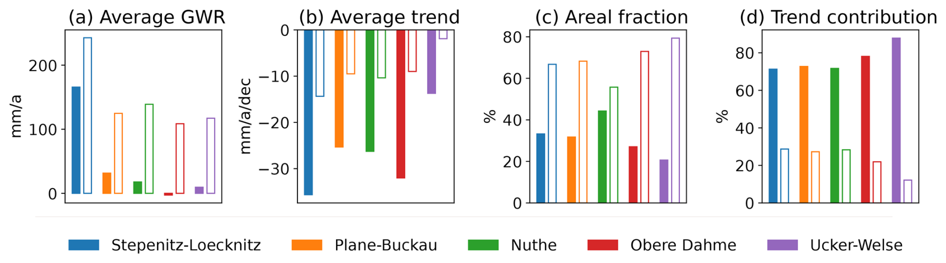
Figure 7 Influence of groundwater depth on average values and trends of GWR in the five study catchments, illustrated for two classes of groundwater depth (filled bars: depth ≤ 3 m; hollow bars: depth > 3 m). The results are based on the observations at the climate stations in Potsdam, Lindenberg, Angermünde, and Marnitz. (a) Area-weighted average of GWR per depth class, (b) area-weighted trend of GWR per depth class, (c) percentage of groundwater depth classes in the catchment area, and (d) relative contribution of each depth class to the overall trend in GWR.

5 Limitations and uncertainties

In the previous section, we demonstrated the interplay of some factors that we expect to govern historical trends in simulated GWR: an increase in potential evapotranspiration (driven mainly by rising air temperature and solar irradiation) translates, particularly in areas with a shallow groundwater table, into a rise in actual evapotranspiration and hence a net decline in GWR at the catchment scale. An increasing LAI further pushes GWR trends towards negative values by enhancing transpiration and interception losses. Yet, these GWR trends are moderated by incoherent positive and negative precipitation trends that, even though not statistically significant, can drive GWR trends in the corresponding direction. As a result, a gap appears to remain between the simulated GWR trends and the more negative trends in observed discharge. What could be the causes behind such a gap? Is it merely an issue of statistical significance, with time series of limited length, or are there any processes not yet sufficiently captured?

Certainly, the chosen approach is affected by various assumptions, simplifications, and uncertainties which might limit the validity of the resulting GWR trends. In the following, we discuss some of these limitations and how to maybe address them in prospective research in order to allow for a more robust answer to our overarching question of why GWR is decreasing in Brandenburg.

5.1 Length of period for trend analysis

In their study using 28 years of groundwater-level data, Lischeid et al. (2021) raised the concern that some of the apparent trends may have been caused by frequency-dependent dampening of low-frequency patterns. In our study, a longer time series of 43 years was used, which should be less likely to be concerned by such an effect. Still, discharge and specifically precipitation exhibit a strong interannual variability so that even longer time series would be desirable for trend analysis. While precipitation observations are available from long before 1980 at a few gauges (see medium-sized triangles in Fig. 6), this is not the case for discharge observations for most catchments in Brandenburg. It should also be noted that we required an exceptionally long spin-up period (from 1951 to 1980), during which the model had to be driven with consistent data in order to properly initialize the deep unsaturated zone.

But even in the presence of longer observational records, it might still be preferable to focus trend analysis on the period since 1980. This is because an overall regime shift appears to have occurred since then (Reid et al., 2016), which implies the coincidence of pronounced trends in not only temperature, but also, for example, solar irradiation (“atmospheric brightening” since the 1980s, after having experienced dimming in the preceding decades), wind speed (“terrestrial stilling”), and LAI (land use changes and “Earth's greening”). Hence, there is a trade-off between getting more robust statistics over longer time periods and the aim to capture the accelerated dynamics of climate change (NOAA, 2023) by putting a stronger focus on recent decades.

5.2 Inhomogeneity of observational series

The observation of all climate variables as well as of discharge can be affected by various sources of inhomogeneities, from changes in the measurement location itself or its surrounding, or changes in the instrumentation (Peterson et al., 1998). In our study, we did not apply any general homogeneity testing or homogenization techniques. Yet, we attempted to minimize some specific sources of inhomogeneity, e.g. with regard to solar irradiation and wind speed (see Sect. 3.2). Still, we consider the uncertainties and the potential for inhomogeneities for these variables to be high. For wind, one alternative would be to use reanalysis data instead of observations. However, initial tests using ERA5-Land data (Muñoz Sabater et al., 2021) showed that these fail in reproducing observed average wind speeds and the effect of terrestrial stilling, which are important aspects with regard to both evapotranspiration and precipitation correction, as demonstrated before.

For precipitation, we applied the correction according to Kochendorfer et al. (2017), which accounts for temperature and wind speed and should hence address inhomogeneities caused by a long-term change in wind-induced undercatch and changing fractions of solid precipitation. Given the uncertainties introduced by the reconstruction of wind data, as well as by changes in instruments and their immediate vicinity, we assume that the precipitation records might still be subject to substantial inhomogeneity (Monika Rauthe, personal communication, 2024). While it will always be difficult to remove such inhomogeneity, it might be possible to identify specifically spurious gauges by homogeneity tests and by investigating station metadata in more detail.

5.3 The role of land cover and vegetation change

Land cover change is known to have a substantial impact on the water balance (e.g. Zhang et al., 2001), so any transient change in land cover can cause a trend in actual evapotranspiration and hence deep percolation and GWR. Land cover change could imply changes in land cover type (e.g. by conversion from forest to agriculture or the reverse) or changes in vegetation properties of an existing land cover type (e.g, by growth or degradation). The transient change in vegetation can act, for example, through a change in LAI (which affects interception, transpiration, and albedo), a change in water-use efficiency due to higher CO₂ levels, or a change in the effective rooting depth (Somogyvári et al., 2024, have confirmed the importance of vegetation changes, as reflected by a changing NDVI, for the dynamics of a groundwater-fed lake system in Brandenburg). While we have shown that, in fact, Brandenburg experienced a significant increase in LAI over the past 40 years, the reasons for this change are not yet understood. Potential hypotheses are forest regrowth (after widespread clear-cuts after World War II), a shift towards maize cropping, a shift towards longer growing seasons due to higher temperatures, or general greening due to increasing CO₂ concentrations (Zhu et al., 2016). However, vegetation changes are not limited to changes in LAI. Rooting depth is another key variable and has a profound effect on transpiration and hence the total water deficit in the soil column before the wintry recharge phase. There is evidence that vegetation can quickly adapt to soil water stress with deeper roots (Fan et al., 2017; Li et al., 2024). A climate-change-induced increase in soil water depletion could hence be amplified by deeper roots, leading to a positive feedback that increases actual evapotranspiration and hence decreases GWR. However, actual observations or even time series are scarce, so any potential trends in rooting depth are almost impossible to quantify for the study area.

5.4 Water consumption by irrigation

Irrigated agriculture is not considered in our model setup; yet, an increase in irrigation water withdrawal or an expansion of irrigated areas could, in theory, contribute to a decline in discharge and groundwater levels. However, there is some evidence that this has not been the case in Brandenburg during the considered time period. Simon (2009) comprehensively reported on the temporal development of irrigated areas and irrigated water volumes in eastern Germany before and after German reunification: in Brandenburg, irrigated areas increased from a value of 1050 km² in 1983 to 1206 km² in 1989 but then collapsed to a value of 200 km² in 1990, followed by more than 30 years in which irrigated areas varied roughly between 200 and 300 km² (309 km² in 2022; see Amt für Statistik Berlin-Brandenburg, 2024). These numbers do not provide any explanation for decreasing discharges: first, irrigated areas decreased by around 80 % after 1990. Second, an irrigated area of 200–300 km² corresponds to a water volume of only 20×10⁶ to 30×10⁶ m³ a⁻¹ (assuming an average annual application of between 70 and 120 mm and its complete evapotranspiration; see Simon, 2009; Amt für Statistik Berlin-Brandenburg, 2012). This volume corresponds to a water depth of around 1 mm a⁻¹ if referred to all of Brandenburg. So even with much higher annual application rates, irrigation dynamics since 1990 do not have the potential to explain any significant part of the observed water balance changes of the past 40 years.

5.5 Direct anthropogenic interventions in the catchments' water balance

As pointed out in Sect. 2.2, we chose catchments and discharge gauges for which we expect direct anthropogenic interference (e.g. by channelized water transfers) with the catchments' water balance to be small. Although we cannot exclude the possibility of such interference, the chances that they will produce more negative discharge trends in all selected catchments are, in our opinion, low. The only catchment for which we actually found a potential effect is the Nuthe catchment: until the 1980s, sewage irrigation fields were operated in the east of the Nuthe catchment near the city of Großbeeren. According to LUA Brandenburg (1997), the corresponding transfer into the Nuthe catchment amounted to around 41×10⁶ m³ a⁻¹, which amounts to roughly 23 mm a⁻¹ at the scale of the receiving Nuthe catchment. While sewage irrigation was discontinued after 1990, it was replaced by a transfer of clear water from the sewage treatment plant, Waßmansdorf, directly into a tributary of the Nuthe. According to Möller and Kade (2005), this transfer nominally amounts to 0.4 m³ under dry conditions and up to 1.3 m³ s⁻¹ under rainfall conditions, corresponding to a range of 7–23 mm a⁻¹ at the catchment scale. Overall, this could imply a maximum decrease in sewage water transfer into the Nuthe after 1990 of up to 16 mm a⁻¹. Referred to the entire period from 1980 to 2023, this could account for a maximum trend component of around −4 of the observed −13 mm a⁻¹ per decade.

5.6 Uncertainties and changes in groundwater depth

Due to permeable soils and low rainfall, actual evapotranspiration in the study area is largely limited by water availability. However, this does not apply in areas with shallow groundwater tables where plants can transpire at maximum rates. Thus, the groundwater depth fundamentally controls the level at which the positive trend in potential evapotranspiration translates into actual evapotranspiration. Any systematic bias in our groundwater depth data would hence propagate to the trend in actual evapotranspiration (although we are not aware of such a bias).

Correspondingly, any temporal dynamics of groundwater depth in areas with shallow groundwater could affect the water balance (be it on the seasonal or decadal scale) and hence also propagate to the trend in actual evapotranspiration. Yet, groundwater tables in areas of shallow groundwater have appeared to be quite stable in the past decades (see Sect. 1) as they are mostly coupled to surface waterbodies and stabilized by their hydraulic regulation.

Some areas with shallow groundwater may be affected by rising groundwater levels after drainage practices have progressively been discontinued over the past 30 years – which would correspond to an increase in actual evapotranspiration. This specifically applies to areas with wetland rehabilitation efforts. For instance, pumping stations have been decommissioned in the Nuthe catchment, leading to re-wetting of areas (LfU Brandenburg, 2025a). At the state level, around 4000 ha of the current total of 6700 ha of wet boglands is based on rehabilitation (LfU Brandenburg, 2025b; MLEUV Brandenburg, 2025). Up to 2045, 188 000 ha of boglands is planned to be restored (MLEUV Brandenburg, 2025). To assess the implications for the state's water balance, prospective research also needs to account for the possibility that a rise of groundwater in a restoration area could propagate beyond its fringes and consequently enhance evapotranspiration at larger spatial extents.

5.7 Model uncertainty

The SWAP model features a large number of parameters, many of which are difficult to quantify and, at the same time, are quite sensitive with regard to the water balance (Wesseling et al., 1998; Baroni and Tarantola, 2014; Stahn et al., 2017). This specifically applies to the soil hydraulic and vegetation parameters (which, for example, control rooting depth and LAI). As pointed out in Sect. 3.4, we did not carry out a calibration but set parameter values from the literature or independent datasets instead. However, Altdorff et al. (2024) used the very same model implementation and confirmed that it could reproduce observed local soil water dynamics in the rooting zone well across eight monitoring locations in Brandenburg (which cover the main land use and soil types as well as shallow and deep groundwater conditions). While this increases our confidence in the model, our implementation of the hydrotope concept is admittedly simple: by considering only two vegetation types (pine forest and grassland/cropland) and one dominant soil type per catchment, specific effects of soils, crop types, or forest traits might not be fully captured by our model setup.

In addition, the uncertainty in soil hydraulic parameters could affect not only the trend of water entering deep percolation, but also the transit times of this water towards the groundwater table (particularly for deep unsaturated zones of several decametres) and hence the temporal distribution of simulated GWR. However, preliminary tests suggested that these delays only have limited effects on the computed trends on the catchment scale. Finally, our model setup does not account for the water flow within the aquifer, which involves an additional dampening of the signal and a further increase in travel time until the water emerges in surface waterbodies.

So while the model itself as well as its setup and parameterization in the context of the present study implies a range of uncertainties, it remains unclear whether and in which direction these uncertainties would affect the simulated trends in GWR. For this purpose, a comprehensive uncertainty and sensitivity assessment with specific attention to GWR trends would be desirable but is beyond the scope of the present study.

6 Conclusions

Time series of river discharge and groundwater levels provide strong evidence that GWR has been decreasing since 1980 in large parts of the federal state of Brandenburg, Germany. So far, however, no simulation study has confirmed any such negative GWR trend.

In our study, we used a combination of model and data specifically tailored to the situation in Brandenburg with its highly permeable soils, low relief, and mix of very shallow and deep aquifers. Furthermore, we paid special attention to using homogeneous climate forcing data, to transparently accounting for the uncertainty in precipitation trends, and, based on a recently published dataset, to considering the effect of a long-term LAI increase on the water balance.

For five catchments across Brandenburg, we found that significant increases in air temperature, solar irradiation, and LAI since 1980 have acted towards a decrease in GWR on the order of −21 to −4 mm a⁻¹ per decade. The contribution of the LAI trend (+0.1 m² m⁻² per decade) amounted to 3–5 mm a⁻¹ per decade. Based on these results, we consider it very likely that the decrease in discharge since 1980 can be explained by a decrease in GWR, which, in turn, was caused by climate change in combination with an increasing LAI.

However, we also found that trends from alternative precipitation times series can be highly incoherent at the catchment scale (partly reaching over more than 20 mm a⁻¹ per decade). Even though none of these precipitation trends is significant, they can have a fundamental impact on the significance, the magnitude, and even the sign of simulated GWR trends.

Given the uncertainty in the precipitation trends, four out of five catchments still appear to exhibit a gap between the negative simulated GWR trends and the more negative observed discharge trends. While we could not explain this gap with certainty, we comprehensively discussed possible reasons, including the effects of the limited length and the inhomogeneity of climate and discharge records, the role of land cover and vegetation change, irrigation water consumption, more latent anthropogenic interventions in the catchments' water balance, uncertainties in groundwater table depth, and model-related uncertainties. Addressing these uncertainties should be a prime subject for prospective research.

Given that the trend in simulated GWR is highly sensitive to any trend in precipitation and that, at the same time, any precipitation trend in future climate projections is known to be highly uncertain and often not significant, we conclude that future projections of GWR trends for Brandenburg need to be interpreted with the greatest caution. Marx et al. (2024) suggested that GWR in Brandenburg will increase in the future; however, the aforementioned discrepancies between models and observations for the past decades do not lend much credibility to such an optimistic outlook.

But what does it mean for water resource management and planning in Brandenburg if we can neither trust in a stable or even increasing GWR nor safely expect a future decrease? Of course, this kind of uncertainty is putting any decision-maker in an inconvenient position. In the light of this uncertainty, our recommendation is to put a stronger focus on monitoring: understanding historical and contemporary dynamics of water availability, based on a combination of models and observations, is our best shot at anticipating critical situations with the required level of certainty. For the current situation, this means that there is very strong evidence that we are in a phase of a climate-induced decrease in GWR, so we should act accordingly.