Exploring implications of input parameter uncertainties in glacial lake outburst flood (GLOF) modelling results using the modelling code r.avaflow

Modelling complex mass flow processes, such as glacial lake outburst floods (GLOFs), for hazard and risk assessments requires extensive data and computational resources. Researchers often rely on low-resolution, open-access datasets and parameters derived from plausibility due to the difficulty involved in conducting direct measurements. This results in considerable uncertainties in forward modelling, potentially limiting the accuracy and reliability of predictions. To determine the sensitivity of the model outputs stemming from input parameter uncertainties in the forward modelling, we selected 9 parameters relevant to GLOF modelling and performed a total of 84 simulations, each representing a unique GLOF scenario in the physically based r.avaflow model. Our results indicate that mass-movement-triggered moraine-dammed GLOF modelling outputs are notably sensitive to five parameters, which are, in order of importance: (1) volume of mass movement entering the lake, (2) DEM datasets, (3) origin of mass movement, (4) entrainment coefficient, and (5) basal friction angle. The GLOF output parameter resulting from the volume of mass movement entering the lake has the greatest coefficient of variation (CV) (47 %), while the internal friction angle had the lowest CV (0.4 %). For future GLOF modelling, we recommend carefully considering the output uncertainty stemming from the sensitive input parameters identified here, some of which cannot be constrained before a GLOF and which must be addressed using statistical approaches.

1 Introduction

Glacial lakes can store millions of cubic metres of water (Zhang et al., 2024, 2023a; Shugar et al., 2020): as of 2020, it is estimated that glacial lakes (0.002 km²) store about 1280.6 ± 354.1 km³ of water around the world (Zhang et al., 2024). The glacial lakes in High Mountain Asia (HMA) have experienced the greatest expansion (46 %) between 1990 and 2018 (Shugar et al., 2020). Furthermore, over 28 % of glacial lakes in HMA are dammed by loose/destabilizing moraines (Fujita et al., 2013; Zheng et al., 2021b) and the majority of glacial lakes (70 %) are exposed to mass inputs in the form of ice/snow avalanches, rockfalls, and landslides from the surrounding slopes (Dubey et al., 2023). Meltwater resulting from the shrinkage of glaciers leads to the formation of new glacial lakes and the expansion of existing ones (Zhang et al., 2015; Wang et al., 2020). This process sometimes exposes them to mass movement from the slopes above and increases the total volume of stored water (Rounce et al., 2016). Additionally, the degradation of permafrost destabilizes the slopes surrounding the glacial lakes, increasing the likelihood of mass movement entering the lake (Huggel, 2009).

Recent work has documented 3151 glacial lake outburst flood (GLOF) events between 850 and 2022 CE globally (Lützow et al., 2023) and 682 GLOF events in HMA between 1833 and 2022 (Shrestha et al., 2023). In HMA alone, these GLOF events have resulted in 6907 human deaths (Allen et al., 2015) and caused damage to more than 2200 buildings, 71 km² of agricultural land, 163 MW of hydropower capacity, 2000 heads of livestock, and numerous other structures including bridges and roads (Shrestha et al., 2023). However, the reported deaths and damage are significantly underestimated because of patchy documentation (Carrivick and Tweed, 2016). The risk from GLOFs is expected to rise in the future with the anticipated expansion of glacial lakes (Zheng et al., 2021b; Zhang et al., 2023b) compounded by a growing population and the construction of structures in areas prone to GLOFs (Taylor et al., 2023; Nie et al., 2023).

Most GLOF events in HMA start with mass movements entering the lake from surrounding slopes, leading to the displacement of water and waves overtopping the dam (Shrestha et al., 2023; Lützow et al., 2023; Nie et al., 2018). Mass movements such as rock or ice avalanches and landslides entering the lake constitute 70 % of known causes of historical HMA GLOF events (Shrestha et al., 2023). The overtopping waves cause moraine dam incision and dam failure, resulting in a sudden discharge of lake water. To a lesser extent, GLOF events are also triggered by factors such as excess hydrostatic pressure from runoff snow and ice melt, intense rainfall and cloud outbursts, and dam settling caused by the melting of ice cores or internal piping. However, it is important to note that, in some cases, these triggering factors may not necessarily result in a complete moraine dam failure. As the flood propagates further downstream, it can transform into a debris flow and/or a hyper-concentrated flow depending on the geologic and topographic characteristics of the river channel as well as depending on the availability of erodible sediment and its grain size distribution (GAPHAZ, 2017; Schneider et al., 2014; Westoby et al., 2015; Westoby et al., 2014). These complex GLOF process chains are difficult to accurately capture in numerical models, given the large number of processes and parameters, which limits our ability to model the impacts of the hazard cascade as a whole.

Numerical modelling of GLOFs

Previous studies have used various modelling codes such as HEC-RAS (Sattar et al., 2021b), BASEMENT (Worni et al., 2013, 2012; Byers et al., 2018), FLO-2D (Somos-Valenzuela et al., 2015), RAMMS (Lala et al., 2018), and r.avaflow (Mergili et al., 2020b). Most of these codes, however, cannot model the evolution of the GLOF process chain through interaction at the boundary of different processes involved (e.g. the interaction of mass movements with the lake) and dynamic transformation of flow through sediment entrainment and deposition. To address this limitation, some of the studies modelled each component separately and then fed the results of each modelling component into the next stage (Lala et al., 2018; Schneider et al., 2014; Frey et al., 2018). For example, Lala et al. (2018) have used RAMMS to model mass movement from the surrounding slope into the Imja Lake, Nepal; the Heller–Hager model and BASEMENT to model wave propagation across the lake surface; and BASEMENT to model the subsequent downstream hydrodynamic evolution of GLOFs. In contrast, the r.avaflow model (Mergili et al., 2017; Mergili and Pudasaini, 2024) enables the integration of all components of the GLOF process chain and their interactions and transformation without the need to combine the results of different models. It enables the detailed modelling of the GLOF process chain, covering everything from the initial trigger to the downstream propagation. r.avaflow is an open-source, GIS-based tool for simulating mass flows over arbitrary terrain. Furthermore, r.avaflow allows for modification of all input parameters, which sets it apart from many modelling codes (where most of the parameters remain hidden within a “black box”), making it suitable for conducting GLOF parameter sensitivity analysis (Mergili et al., 2017; Mergili and Pudasaini, 2024).

r.avaflow utilizes the total variation diminishing non-oscillatory central differencing (NOC-TVD) numerical scheme (Wang et al., 2004) to solve an enhanced version of the Pudasaini multiphase flow model (Pudasaini and Mergili, 2019). It also offers added features for entrainment, deposition, dispersion, and phase transformation. Because of these features, r.avaflow can model the full process chain of a GLOF and flow transformation due to erosion of bed material and deposition of entrained material (Mergili et al., 2017; Mergili and Pudasaini, 2024). However, the precision of this model output parameters such as peak flow, depth, and velocity depends on the accuracy of various input parameters and initial conditions, such as the release volume of mass, the resolution and vertical accuracy of the digital elevation model (DEM), density, entrainment, and frictional parameters (Mergili et al., 2017).

Because of the significant logistical challenges associated with collecting field data and the financial costs involved in acquiring high-resolution remote sensing data, many of the parameters in GLOF modelling are derived from open-access data, leading to considerable uncertainties in the resultant discharge, inundation extent, and arrival times. Also, certain input parameters such as the volume of mass movement entering the lake are impossible to measure accurately before a GLOF event. For example, the global-scale DEM SRTMGL1 (Shuttle Radar Topography Mission Global 1 arcsec), with a ground resolution of 30 m, is commonly employed in GLOF modelling without adequately considering the inherent uncertainty due to horizontal and vertical inaccuracies in this DEM (Rinzin et al., 2023). Similarly, the origin of avalanches and other mass movements is determined using low- to medium-resolution remote sensing imagery and DEMs, often supplemented by secondary datasets like permafrost data (Obu et al., 2019), which can introduce notable uncertainties (Sattar et al., 2023; Allen et al., 2016). When estimating the volume of avalanches entering the lake, DEM differencing between pre- and post-event conditions can be advantageous for reconstructing historical events (Baggio et al., 2021; Zheng et al., 2021a), although the accuracy is contingent upon the vertical and horizontal accuracy and resolution of the data and the temporal interval between data acquisition. Likewise, when ice is considered the sole source of the mass movement, ice thickness is employed to calculate the avalanche volume (Allen et al., 2022), for which the accuracy of the computed volume relies on the resolution and availability of ice thickness data from the ice-flow inversion model in the region of interest. When the depths of landslides and avalanches are not known, arbitrary thicknesses of 10, 30, and 50 m based on past events (Dubey et al., 2023) are often utilized for forward modelling, further contributing to significant uncertainties in the modelling results (Rounce et al., 2017, 2016; Dubey and Goyal, 2020).

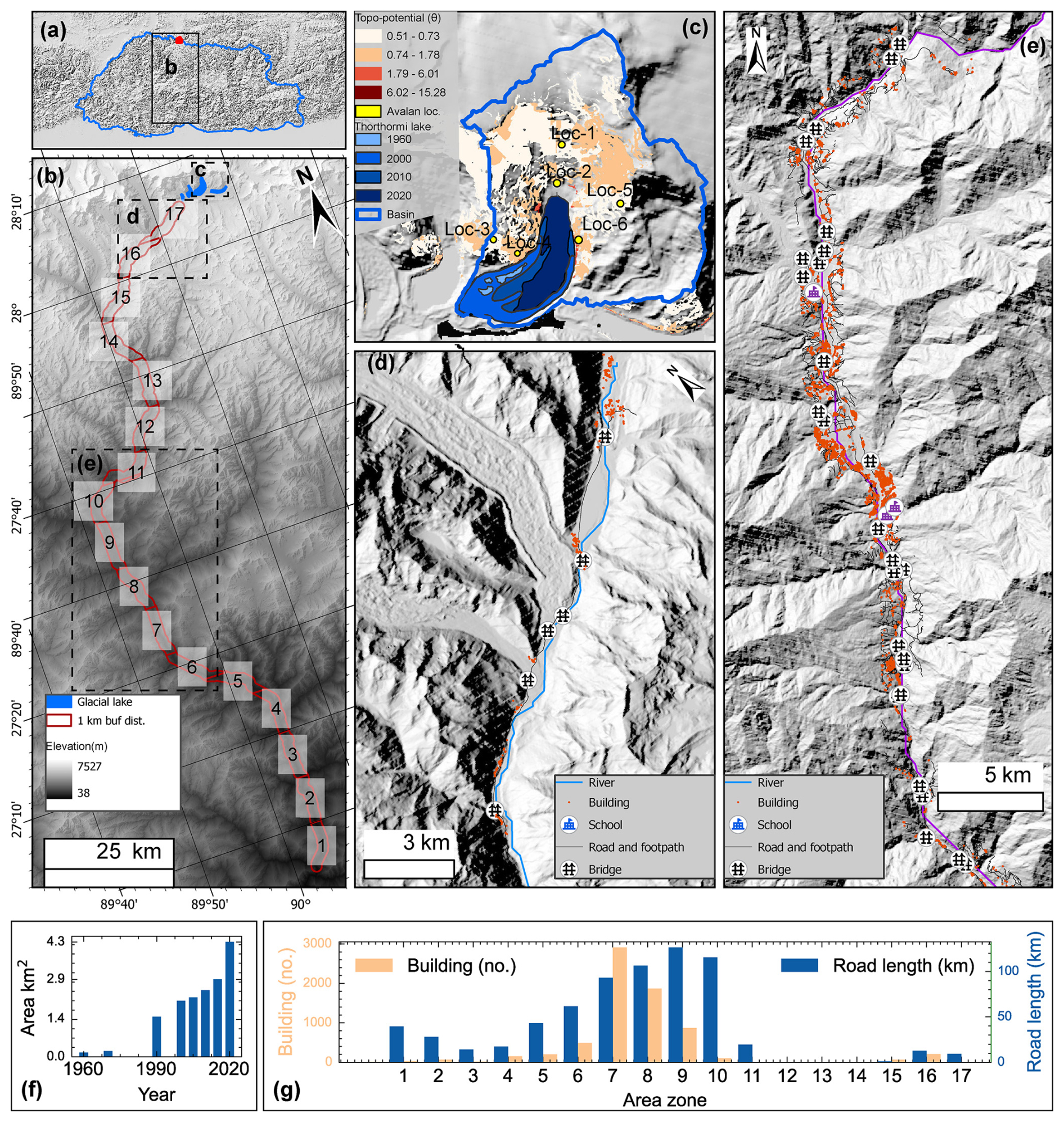
Figure 1 Study area. (a) The location of Thorthormi Tsho and its downstream condition in Bhutan. (b) Elevation (as per SRTMGL1) and the overview of glacial lakes in Lunana and settlements along the Phochu and Punatsangchu basins, downstream of Thorthormi Tsho. The downstream settlement is divided into 17 zones (1–17), each 10 km long. (c) Area of Thorthormi Tsho between 1960 and 2020 and the surrounding slope with topography potential (TPP) for mass movement entering Thorthormi Tsho. The downstream settlements in the (d) Lunana and (e) Punakha and Wangdue Phodrang regions. (f) The change in the area of Thorthormi Tsho between 1960 and 2020 (Rinzin et al., 2023) and (g) the buildings (count) and road (km) within 1 km on either side of the river centreline as per the latest version of OpenStreetMap (as of 30 March 2024). Loc-1 to Loc-6 are the locations of the origin of mass movement entering the lake considered for this study. The background map for the panels is hillshade from SRTMGL1.

Moreover, the flow parameters in r.avaflow are adjusted and optimized based on the fit of the model's results to well-documented past events (Mergili et al., 2017, 2020a; Vilca et al., 2021) and the physically plausible range suggested by Mergili et al. (2017, 2018a, b). Efforts to fine-tune parameters to fit with historical events of varying magnitude, temporality, and spatiality have led to the use of wide-ranging values. For example, Mergili et al. (2020b) used an internal solid friction angle of 28° to reconstruct the 1941 GLOF process chain of Lake Palcacocha in the Cordillera Blanca, Peru. In contrast, Vilca et al. (2021) used 45° to model the 2020 glacial lake outburst process chain of Lake Salkantaycocha located in Cordillera Vilcabamba of Peru. Likewise, the value of the basal friction angle ranges between 6–18° (Baggio et al., 2021; Mergili et al., 2020a) (Supplement Fig. S1). Because each GLOF event is inherently distinct, even when originating from the same glacial lake (Emmer and Cochachine, 2013; Lala et al., 2018), inferring reconstructed values from past events for forward modelling introduces substantial uncertainties (GAPHAZ, 2017; Mergili et al., 2020b). Finally, r.avaflow model outputs are extremely sensitive to parameters like the entrainment coefficient value, basal friction angle, and initial release volume (Mergili et al., 2018b, a; Baggio et al., 2021). While all these indicate that the value of input parameters is highly variable depending on specific events, to our knowledge, how changes in the values of these input parameters affect the model output (for example, peak and total flow, flow depth, flow velocity, and arrival time) is not known.

To determine the relative contribution of uncertainties in different input parameters to variability in GLOF extent, we identified 9 out of 38 input parameters and initial conditions relevant to GLOF flow modelling: digital elevation model, the volume of mass movement entering the lake, the origin of mass movement entering the lake, grain density of mass movement entering the lake, volume of the lake, entrainment coefficient, internal friction angle, basal friction angle, and fluid friction number (Table S1 in the Supplement). Our selection was motivated by the recognition that these input parameters are considered essential and have been frequently adjusted in previous studies to align with values inferred from the observed past events (Baggio et al., 2021; Mergili et al., 2018b; Allen et al., 2022; Zheng et al., 2021a; Vilca et al., 2021). We believe that these parameters are the most likely to influence the results of future modelling efforts, making it critical to evaluate their impacts on model outputs. We assessed the sensitivity of the model output to each of these parameters by conducting up to 10 r.avaflow simulations per parameter and varying their values within the range determined from the literature that employed r.avaflow modelling (Fig. S1). We investigated the impact of variation of these parameter values on the model outputs and used the following diagnostic variables: peak discharge, total discharge, flow arrival time, flow depth, flow velocity, and reach distance. We then calculated the coefficient of variation for each parameter and ranked them based on this metric.

2 Study site

Here, our sensitivity analysis was conducted on Thorthormi Tsho (28.10° N, 90.27° E) located in the Lunana region of the Bhutan Himalaya (Fig. 1). The area of Thorthormi Tsho has expanded by ∼ 192 % since 1990, evolving into the largest proglacial lake (area of 4.35 km²) in Bhutan by 2020 (Rinzin et al., 2023) (Fig. 1b and f). Although the lake level was lowered by 5 m by artificially draining out the water between 2008 and 2012 (NCHM, 2019a), Thorthormi Tsho is considered the most dangerous glacial lake as it is determined to be susceptible to triggering factors (like mass movement entering the lake) and potentially unstable moraine damming the lake (NCHM, 2019a; Rinzin et al., 2021) (Fig. 1b). In recent years, Thorthormi Tsho has produced two GLOF events (NCHM, 2023), with the first occurring on 20 June 2019 (NCHM, 2019b) and the latest occurring on 30 October 2023. Also, modelling of future predicted GLOFs from Thorthormi Tsho shows it can produce a flood with flow volume of up to 3 × 10⁸ m³ of water with a peak discharge of up to 75 000 m³ s⁻¹, affecting more than 16 000 people and various infrastructure downstream of this glacial lake (Rinzin et al., 2023). This high level of outburst susceptibility and hazard makes Thorthormi Tsho an ideal candidate for GLOF modelling to improve our modelling output of GLOF uncertainty.

Additionally, the Phochu and Punatsangchu basins, located downstream of Thorthormi Tsho, are the most populated basins in Bhutan. The latest updated version of OpenStreetMap (https://www.openstreetmap.org, last access: 30 March 2024), although it does not have 100 % coverage, shows that there are over 7000 buildings, 50 bridges, 4 schools, 687 km of road, and a large area of agricultural land within a 1 km radius of the Phochu and Punatsangchu rivers (Fig. 1c, d, g). Besides, located downstream are the two biggest hydropower plants (Punatsangchu-I and Punatsangchu-II) in Bhutan, poised to become key contributors to the nation's gross domestic product (GDP). Also, the Punakha Dzong, which has great historical and cultural significance to Bhutan, is located downstream of Thorthormi Tsho. This high downstream exposure to GLOF hazard further highlights the importance of understanding GLOF characteristics from Thorthormi Tsho (Fig. 1).

3 Methods

3.1 r.avaflow model framework

r.avaflow is a comprehensive GIS-based open-source computational framework for modelling mass movement from one or more release areas over the defined basal topography (Mergili et al., 2017; Mergili and Pudasaini, 2024). It can model the entire GLOF process chain from the release of avalanches through the dynamic interaction of the avalanche and lake water and overtopping and retrogressive moraine dam erosion and finally to the downstream evolution of the resulting flow (Mergili et al., 2020b; Vilca et al., 2021; Sattar et al., 2023). It can also robustly consider the interactions between the phases as well as erosion and deposition (Mergili et al., 2017). Furthermore, it is equipped with a built-in function for visualization and validation. Because of this capability, r.avaflow has been widely used to model process chains such as GLOFs in high mountains all over the world, mostly to reconstruct past events (Zheng et al., 2021a; Mergili et al., 2020b; Vilca et al., 2021) and to a lesser extent to predict future hazards (Sattar et al., 2023; Allen et al., 2022).

In r.avaflow, the evolution of the flow in space and time is solved using an enhanced version of the Pudasaini multiphase flow model (Pudasaini and Mergili, 2019; Pudasaini, 2012). The flow is computed through depth-averaged conservation of mass and momentum equations for solid and fluid components. These equations involve six differential equations accounting for solid (D_s) and fluid (D_f) flow depths, solid (M_sx) and fluid (M_fx) momentum in the x direction ($M_{\mathrm{s}x}=D_{\mathrm{s}}\times v_{\mathrm{s}x},M_{\mathrm{f}x}=D_{\mathrm{f}}\times v_{\mathrm{f}x}$), and M_sy and M_fy in the y direction ($M_{\mathrm{s}y}=Ds\times v_{\mathrm{s}y},M_{\mathrm{f}y}=D_{\mathrm{f}}\times v_{\mathrm{f}y}$, where v is the flow velocity) (Mergili et al., 2017). Mohr–Coulomb plasticity is used to compute solid stress, while fluid is subjected to solid volume-fraction-gradient-enhanced non-Newtonian viscous stress. r.avaflow also considers other factors like virtual mass force, viscous drag, and buoyancy. These factors collectively facilitate momentum transfer between the solid and fluid phases, enabling the simultaneous deformation, separation, and mixing of phases as they propagate across the mountain topography (Pudasaini and Mergili, 2019; Pudasaini and Krautblatter, 2014b; Mergili et al., 2020b; Pudasaini, 2012). To numerically solve these differential equations and propagate flow over time and space, r.avaflow uses a high-resolution total variation diminishing non-oscillatory central differencing (TVD-NOC) scheme, a commonly used numerical scheme to handle the advection of quantities, whilst minimizing numerical artefacts like oscillations (Wang et al., 2004). The internal friction angle and basal friction angle, which are crucial factors governing the frictional forces influencing flow rheology, are adjusted based on the solid fraction of the flow material (Mergili et al., 2018b, 2017; Pudasaini and Mergili, 2019).

r.avaflow has three different models, namely, a single-phase shallow-water model with Voellmy friction relation, an enhanced version of the multiphase flow model of Pudasaini and Mergili (2019), and an equilibrium-of-motion model for slow-flow process (Mergili and Pudasaini, 2024). Here, we chose an enhanced version of the multiphase flow model considering an erodible moraine dam and mass movement entering the lake as the solid component and lake water as the fluid component. The multiphase mass flow model can simulate the propagation of three different elements – solids (coarse material including boulders, cobbles, and gravel), fine solids (including sand and particles larger than clay and silt), and fluids (including water and very fine particle including clay, silt and colloids) – and assign each of them a distinct flow rheology (Pudasaini and Mergili, 2019).

Furthermore, r.avaflow has six specific optional functions including conversion of release height to depth, diffusion control, surface control, entrainment, stopping, and dynamic adaption of frictional parameters. The latest version of r.avaflow has four options to compute erosion and entrainment: (i) a model calculated by multiplying the entrainment coefficient with flow momentum, (ii) a simplified entrainment–deposition numerical model of Pudasaini and Krautblatter (2014a), (iii) a combination of models i and ii, and (iv) an acceleration–deceleration entrainment and deposition model. Since models ii to iv are in the experimental phase, here, we used model i, where the amount of entrainment is computed dynamically by multiplying with the user-defined entrainment coefficient (C_E) with the total momentum of the flow at the given raster cell and time step (Mergili et al., 2017) (Eqs. 1 and 2).

$$\begin{array}{}\text{(1)}& {\displaystyle }{q}_{\mathrm{E},\mathrm{s}}=C_{\mathrm{E}}|M_{\mathrm{s}}+M_{\mathrm{f}}|{\mathit{\alpha }}_{\mathrm{s},\mathrm{Emax}},\text{(2)}& {\displaystyle }{q}_{\mathrm{E},\mathrm{f}}=C_{\mathrm{E}}|M_{\mathrm{s}}+M_{\mathrm{f}}|(\mathrm{1}-{\mathit{\alpha }}_{\mathrm{s},\mathrm{Emax}}),\end{array}$$

where q_E,s and q_E,f are the entrainment rates of solids and fluids, respectively; C_E is user-defined entrainment coefficient (kg⁻¹); and α_s,Emax uses user-defined the solid entrainable material height (m).

We utilized r.avaflow direct, a web-based tool (Mergili and Pudasaini, 2024), to initially generate the sample model script. We modified the sample script by inputting parameters relevant to each experimental set-up and wrote a Bash shell script for all simulations in each experiment to test various parameter values within our predefined range. We developed one master Bash script for each experiment that allowed us to run all experiments in parallel, leveraging the Rocket high-performance computing (HPC) facilities at Newcastle University. All the GLOF simulations were done for Thorthormi Tsho and were run for 1500 s when the flow reached up to ∼ 24 km downstream of the lake, depending on values of various parameters defined here. The flow propagation beyond this point and its interaction with the downstream component are beyond the scope of this study.

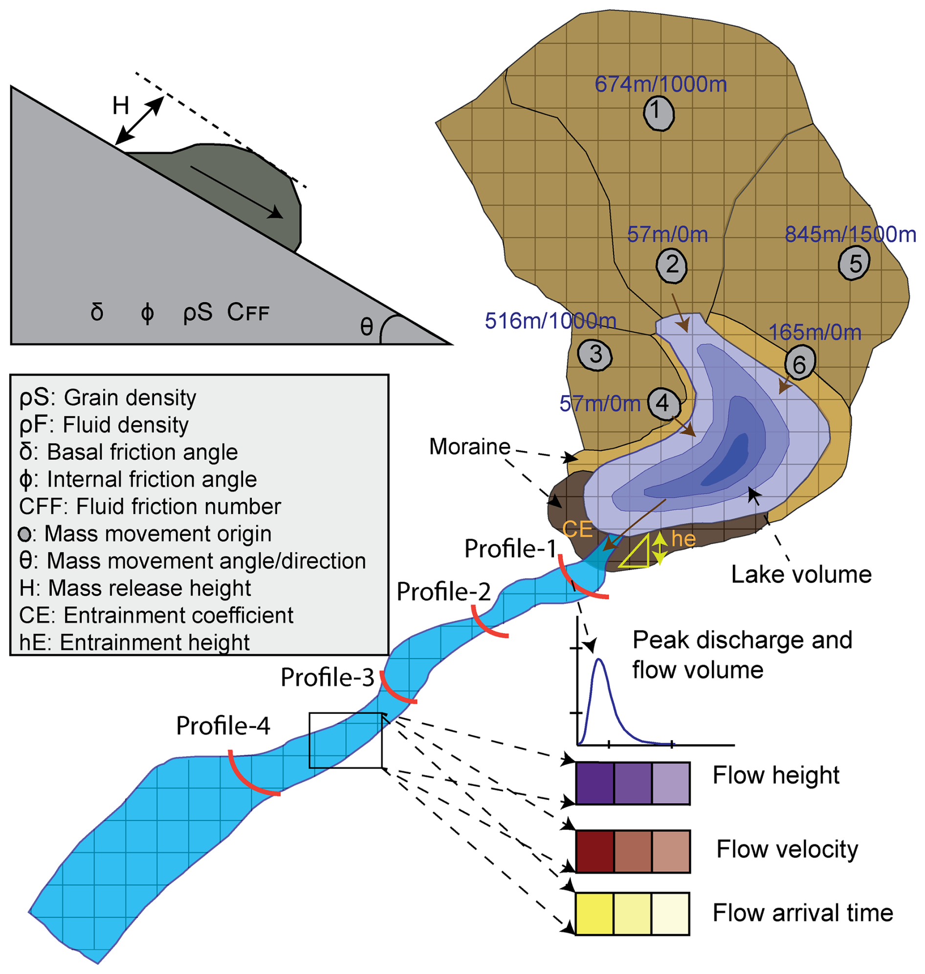
Figure 2 Schematic view of Thorthormi Tsho, surrounding terrain (study area) and input parameters employed for investigating r.avaflow model output sensitivity used in this study. Points 1–6 show the origin of mass movement entering the lake (considered for this study) with the vertical drop and horizontal distance (separated with a slash) to the lake shoreline.

Table 1 Key parameters tested in this study to investigate model output sensitivity. Detailed parameters for r.avaflow modelling are provided in Table S1. The constant value is the common parameter value used across experimental setups.

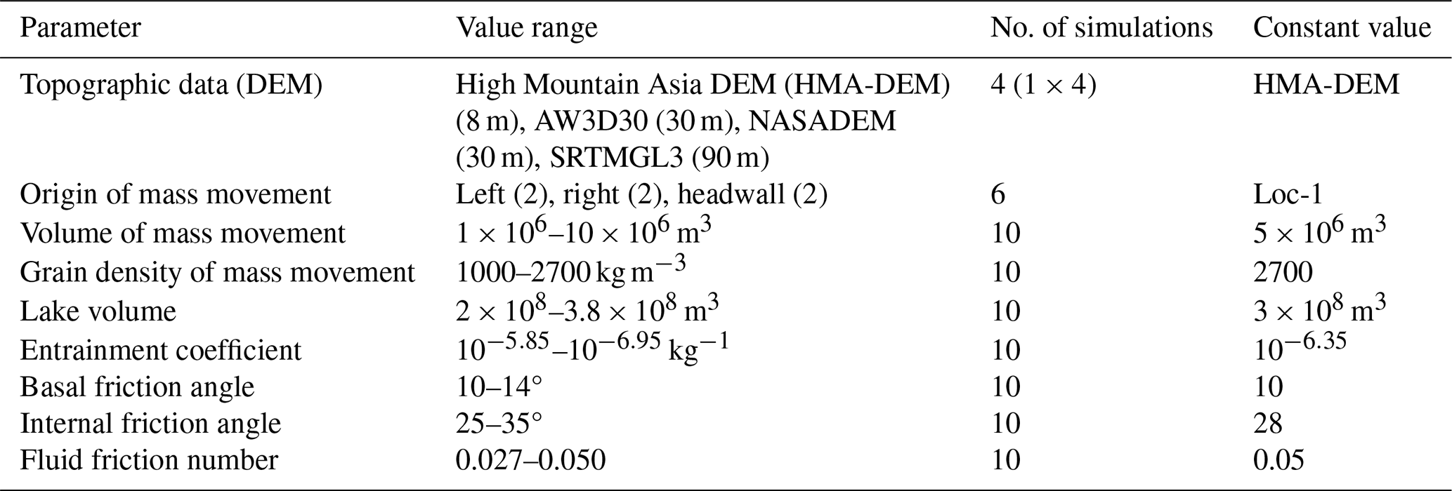
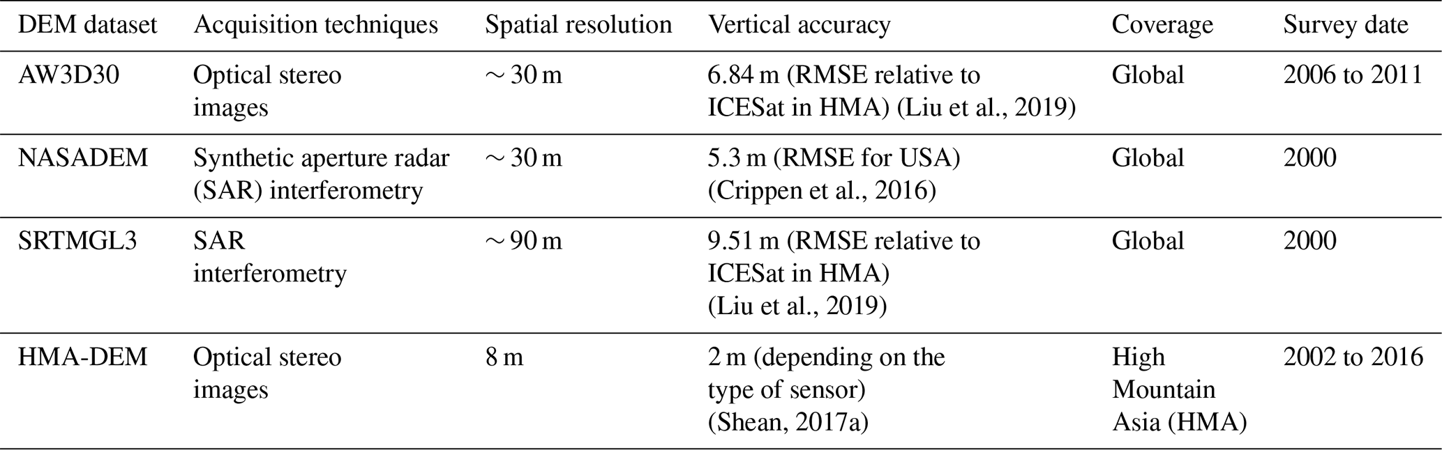
Table 2 Characteristics of DEM datasets employed in this study to investigate the impact of DEM dataset variation on GLOF modelling results.

3.2 Model input parameterization and experimental setups

In the context of r.avaflow, a parameter is a (often user-defined) variable influencing the physical characteristics of the movement or the numerical behaviour of the flow. Parameters can be based e.g. on physics (such as friction angles) or empirical knowledge. Parameters can be represented by global values, by individual values for each raster cell, or by time-dependent values. r.avaflow has a large choice of parameters and initial conditions, such as a DEM representing initial basal topography, the volume of the solid and liquid phase, entrainment and stopping parameters, and density and frictional parameters (Mergili and Pudasaini, 2024) (Table S1). The values specified for these parameters influence crucial aspects of modelled GLOF flow characteristics, including the impacted area, travel distance, travel time, and volume of sediment deposited at the various downstream locations (Mergili et al., 2017). In this study we selected a total of nine parameters which are identified as important and commonly modified in the previous studies (e.g. Mergili et al., 2020a): (1) DEM dataset, (2) volume of mass movement entering the lake (V_S), (3) origin of mass movement entering the lake, (4) volume of the glacial lake (V_L), (5) grain density of mass movement entering the lake (ρS), (6) entrainment coefficient (C_E), (7) basal friction angle (δ), (8) internal friction angle (ϕ), and (9) fluid friction number (C_FF). To investigate the impact of DEM dataset variation, we modelled GLOFs by employing freely available global and regional DEM datasets with differing spatial resolution and vertical accuracy (Table 2). For the origin of mass movement entering the lake, we first computed the topographic potential for mass movement entering the lake (Allen et al., 2019) (Fig. 1b) and selected six different sites by considering the topographic potential values and geometry of the lake (Fig. 2). The V_S was varied between 10⁶–10⁷ m³. The ρS value range was considered based on assumed combinations of rock and ice parts in mass movement following the approach used in the earlier studies (Allen et al., 2022; Sattar et al., 2023). For parameters 5–9, we gathered various values employed in previous studies (Allen et al., 2022; Mergili et al., 2020a, b; Vilca et al., 2021) and computed descriptive statistics and established the median, upper quantile, and lower quantile for each parameter using these collated values (Fig. S1). We then varied these parameter values between the calculated upper quartile and lower quartile, yielding 10 equally spaced values in total. This range of 10 values was utilized in a total of 10 experiments for each respective parameter whilst holding other parameter values constant at the median value. For example, for the ϕ experiment, the value of ϕ was varied between the upper and lower quantiles, with 10 increments in total, whilst holding constant the other parameter values (Table 1). An overview of the employed parameters and workflow is shown in Fig. 2 (schematic view) and Table 1, while further details on the parameter range used for each experiment are provided in the following section.

3.2.1 Digital elevation model

Here our goal is to constrain model output uncertainty stemming from the use of freely available global and regional DEM datasets. We performed a series of GLOF simulations using four open-access DEM data sources of various resolutions, vertical accuracy, and elevation derivation methods, namely, the High Mountain Asia DEM (HMA-DEM; 8 m) (Shean, 2017), ALOS (Advanced Land Observing Satellite) global digital surface model (AW3D30; 30 m) (JAXA, 2021), NASADEM (∼ 30 m) (NASA JPL, 2021), and SRTMGL3 (∼ 90 m) (SRTM, 2013) (Table 2). The details about the DEM datasets used here are provided in the Supplement.

3.2.2 Volume of the glacial lake and mass movement entering the lake

r.avaflow has the option to define the initial release volume of different phases involved in the GLOF process chain. Here, we assume the GLOF was initiated by rock–ice-mixed mass movement entering the lake followed by a tsunami wave hitting the moraine, damming the lake and causing moraine dam failure. Accordingly, we defined the frontal moraine damming Thorthormi Tsho as phase 1 (rock component with ρ=2700 kg m⁻³), mass movement entering Thorthormi Tsho as phase 2 (rock–ice component), and Thorthormi Tsho as phase 3 (fluid part).

Field-based bathymetric data are essential for accurately estimating V_L, which is a fundamental input for the GLOF modelling. However, the remote and harsh environment of glacial lakes in the mountain regions makes it highly challenging to conduct field-based bathymetric surveys. In the case of Thorthormi Tsho, conducting the bathymetric survey is particularly difficult as the lake is filled with debris and icebergs, which makes it hazardous to conduct a survey. In the absence of field-based bathymetry, the area–volume empirical equations are commonly employed by past studies to approximate V_L. However, these area–volume scales are based on sparse field data and may not represent the actual volume, leading to substantial uncertainties in the volume estimates (Zheng et al., 2021a; Gantayat et al., 2024). In this study, we calculated the volume of Thorthormi Tsho considering eight area–volume empirical equations which are commonly used for computing the volume of moraine dam lakes (Table S2). Uncertainty in using these empirical equations where evident as the V_L estimate for Thorthormi Tsho ranges between 2.1 × 10⁸ and 3.8 × 10⁸ m³. So, to investigate the impact of this uncertainty in modelled GLOF hydraulics, we modelled 10 scenarios of GLOFs by varying V_L from 2.0 × 10⁸ to 3.8 × 10⁸ m³ with increments of 20 × 10⁶ m³. For all other experiments, the median value (2.9×10⁸ m³) of V_L estimated from area–volume scaling equations was used uniformly. r.avaflow requires spatially varying lake bathymetry to be used as fluid release height rather than the absolute V_L. With Thorthormi being a recently formed lake, it has ice thickness data covering the extent of the lake (Farinotti et al., 2019). Therefore, we computed the bathymetry of Thorthormi Tsho by subtracting ice thickness data from the surface DEM (Linsbauer et al., 2016, 2017). Assuming that the present-day lake has been formed by filling the overdeepening, this ice-thickness-derived bathymetry was adjusted to match the volume we employed for each modelled GLOF. For example, for the experiment with a V_L of 3 × 10⁸ m³, the ice thickness bathymetry was adjusted to get the same volume (Table S2).

The volume of mass movement entering the lake serves as a fundamental parameter for defining various scenarios in the forward modelling of a GLOF (for example, Allen et al., 2022, and Sattar et al., 2023). However, it is difficult to predict how big or small the mass movement will be. The historical record of V_S is sparse but mostly exceeds 1×10⁶ m³ (for example, Zheng et al., 2021a, and Byers et al., 2018), although a recent event in Sikkim Himalaya was known to have been caused by a volume of up to 14.7×10⁶ m³ (Sattar et al., 2025). Additionally, earlier studies in Nepal based on topographic potential and assumed three depths based on avalanches in Russia and the Swiss Alps (10, 30 and 50 m) (Rounce et al., 2016) has estimated the volume between 2.7 × 10⁶ to 6.7 × 10⁶ m³. Here we selected the most likely zone of mass movement entering the lake based on the topographic potential of the slope surrounding the lake. However, accurately constraining V_S remains highly challenging and subject to considerable uncertainty. Considering these uncertainties, to test the effect of mass movement of various volumes, we conducted a series of 10 experiments considering V_S ranging from 1×10⁶ to 10×10⁶ m³. For the other experiments, we used a uniform V_S of 5 × 10⁶ m³ (Table 1).

3.2.3 Origin of mass movement entering the lake

To account for uncertainties involved in the origin of mass movement entering the lake, we identified a total of six mass movement areas, each characterized by different directions and distances to the lake (Figs. 1 and 2). To do this, we first computed topographic potential for mass movement (rock–ice avalanche and landslide) entering the lake based on slope and runout trajectory criteria (Allen et al., 2019). Based on this first-order estimate, we identified the six potential instances of origin of mass movement each with a unique direction, height, and distance relative to the lake (Fig. 2): Loc-1 (slope ∼ 1 km away from the headwall, aligned along the longitudinal axis of the lake), Loc-2 (headwall about 100 m away from the lake along the longitudinal axis), Loc-3 (slope 1 km from the right moraine dam), Loc-4 (right moraine dam), Loc-5 (slope ∼ 1.5 km from the left moraine dam), and Loc-6 (left moraine dam) (Figs. 1 and 2). We then ran one scenario of a GLOF from each of these locations (total of 6), keeping all input variables constant for each model run. For the rest of the experiments, we used a mass movement scenario from Loc-1.

3.2.4 Grain density of mass movement entering the lake

Our goal here is to assess the impact of ρS entering the lake, which serves as a proxy for the ice-to-rock ratio. Accordingly, we consistently set the grain density of phase 1 (moraine) at 2700 kg m⁻³ across all the experiments, whilst the fluid density of phase 3 was also held constant at 1000 kg m⁻³. In the earlier studies, ρS had been used as a proxy for the portion of a rock–ice component of mass movement entering the lake, which is highly uncertain (Vilca et al., 2021; Allen et al., 2022). The phase separation of rock and ice components of the mass movement with different densities is not well established in r.avaflow (Vilca et al., 2021). Therefore, in this study, following Sattar et al. (2023), a portion of snow and ice in the mass movement is considered fluid by adjusting the ρS of the phase 2 represented by the mass (Table S3). In our experiment set-up, this is executed by varying the ρS value between 2700 kg m⁻³ (representing 100 % rock) and 1000 kg m⁻³ (representing 100 % ice) (Table 1).

3.2.5 Entrainment coefficient

Material entrainment due to bed erosion can make the flow more concentrated and thus increase the volume, resulting in spatial and temporal variation in flow. In the r.avaflow model, the user must define entrainment height in the form of a raster covering the entire model domain, which can be identified using either remote sensing imagery or fieldwork (Mergili and Pudasaini, 2024). However, accurately measuring the depth and spatial extent of these erodible materials covering the entire model domain is highly challenging, even with field surveys, and remains infeasible using remote sensing techniques alone. In this study, we focused on the frontal moraine, as it is measurable using remote sensing data. The extent of the moraine was mapped using high-resolution Google Earth imagery, while its height was determined using HMA-DEM (Fig. 1). The amount of entrainment itself is dependent on the user-defined C_E. In r.avaflow the base-10 logarithm of C_E must be entered (Mergili et al., 2018a, 2017). Here, we modelled 10 scenarios of GLOFs by varying C_E between 10^−6.95 and 10^−5.85 kg⁻¹ (Table 1).

3.2.6 Frictional parameters

The internal friction angle (ϕ), basal friction angle (δ), and fluid friction number (C_FF) mechanically control the basal shear stress, internal deformation, anisotropy of the stresses, and hydraulic pressure gradient of the solid constituents (Pudasaini and Krautblatter, 2014b), which are essential attributes influencing flow runout distance and time. Within the r.avaflow model set-up, a user can use either spatially varying values for these frictional parameters using a raster map or one absolute value (Mergili and Pudasaini, 2024; Mergili et al., 2017). In this study, we computed 10 experiments for each of these frictional parameters. Specifically, by varying ϕ between 25 and 35°, δ between 10 and 14°, and C_FF between 0.027 and 0.050 (Table 1).

3.3 Sensitivity analysis

Here we use sensitivity analysis to determine how variations in the initial values for key input parameters impact the modelled GLOF hydraulics (Saltelli et al., 2004). Thus, our goal is not to determine the “correct” value for each parameter but to determine the r.avaflow input parameter(s) that cause the most variation in the model output. To constrain this variability, we mainly focused on examining the peak discharge, total discharge, and flow arrival time as the output metrics. The flow for all the experiments was measured from the profile immediately beneath the moraine dam (profile 1 in Fig. 2). We calculated the peak and total discharge based on the flow data obtained from the same profiles (Fig. S2). The flow arrival time was considered the average value across the time recorded from the profiles located 3, 6, and 9 km downstream of Thorthormi Tsho (profiles 2, 3, and 4 in Fig. 2). For the scalable parameters, we also computed simple linear regression considering input parameters as the independent variable and model output as the dependent variable. To ascertain the sensitivity of the three model output metrics defined earlier for variations in values across all parameters, we computed the coefficient of variation (CV) for individual parameters and subsequently ranked them based on this metric. The CV is a statistical measurement of the dispersion of data points around the mean, regardless of the units used to measure it. The CV is deemed suitable here since the r.avaflow output variability is caused by input parameters that are measured in different units. To calculate the CV, we took the standard deviation of the output value range of a particular experiment (e.g. peak discharge) and divided it by the mean of the same output range (Abdi, 2010). We multiplied each CV value by 100 to express them in percentage form.

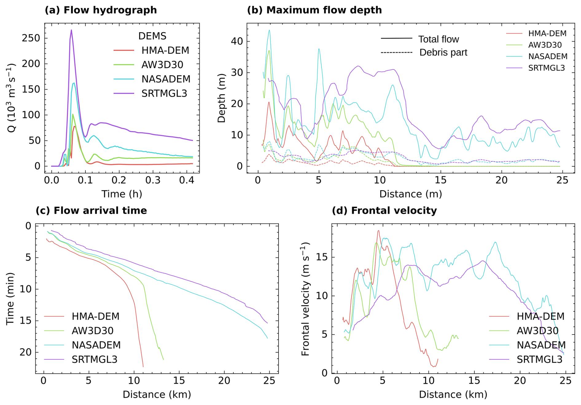
Figure 3 The line graph showing the (a) rate of flow (Q), (b) maximum flow depth (for total and debris part), (c) flow arrival time, and (d) flow velocity profiles along the river centreline generated by conducting a sequence of r.avaflow simulations, employing different types of DEM datasets. The solid and dashed lines (in panel a) show the maximum flow depth and debris part of the flow. The profiles are plotted as rolling averages every 100 m.

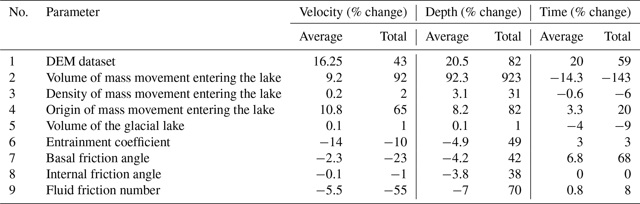
Table 3 Percentage change in flow velocity, depth, and arrival time resulting from variation in values of different input parameters we employed in this study. The total percentage (%) change represents the output variation resulting from the maximum and minimum input parameter values used in the experiment. The average percentage (%) change is calculated as the mean change across all incremental steps employed in setting up the experiment. The arrival time is the average of the record from three locations (profiles 2, 3, and 4) (Fig. 2). Flow velocity and depth are mean values taken from the river centreline. The negative (−) value indicates that increasing input parameters decreases output parameters. The detailed flow pattern along the river centreline is provided in Figs. S3, S4, S5, and S6.

4 Results

4.1 Effect of the DEM dataset

When the GLOF was modelled employing freely available global and regional DEM datasets (HMA-DEM, AW3D30, NASADEM, SRTMGL3), our results showed a variation in peak and total discharge of a GLOF from Thorthormi Tsho by almost 100 % and 400 %, respectively (Fig. 3). Specifically, HMA-DEM consistently produced the lowest-magnitude GLOF, while SRTMGL3 consistently produced the highest. Although NASADEM and AW3D30 have a similar spatial resolution, notable differences (65 %) in peak discharge and other hydraulic properties emerged between simulations done using these datasets (Fig. 3a).

We observed a significant fluctuation in the mean flow depth (82 %) and velocity (43 %) along the flow path resulting from the change in DEM datasets (Table 3). For instance, the mean flow depth along the river centreline ranged from 39 m (HMA-DEM) to 54 m (SRTMGL3) (Table 3) and the flow reach distance increased from 15.5 km (HMA-DEM) to 24.2 km (SRTMGL3). Once again, NASADEM and AW3D30 yielded significantly different maximum flow depths (8.5 %) and reach distances (72 %) (Fig. 3b). The flow arrival time varied by around 59 %. Flows derived from SRTM data always arrived earlier, while those using HMA-DEM were consistently most delayed (Fig. 3c). There was also a similar variation in the solid concentration of the flow in response to changes in input DEM datasets (Fig. 3b).

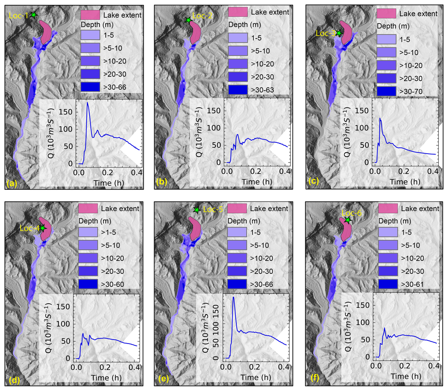
Figure 4 Flow rate and depth resulting from mass movement entering the lake from different locations: (a–f) Loc-1 to Loc-6.

4.2 Effect of the origin of mass movement entering the lake

We modelled mass movement with a volume of 5 × 10⁶ m³ entering the lake from the surrounding slopes at various locations identified in Sect. 3.2.3. Our study found that the GLOF process chain initiated by mass movements from Loc-1 to Loc-6 results in a significant fluctuation in the GLOF output (Fig. 4). The peak discharge varied by approximately 200 %, with the total discharge varying by 55 % (Fig. 4). Likewise, the mean flow depth, velocity, and arrival time fluctuated by 65 %, 82 %, and 20 %, respectively (Table 3). By comparison, the flow resulting from the GLOF initiated by mass entering from Loc-1 (Fig. 4a) (1 km from the headwall) and Loc-5 (∼ 1.5 km above the left moraine) (Fig. 4e) produced the highest-magnitude GLOF, while that from Loc-4 (right lateral moraine) (Fig. 4d) was the lowest. For example, the highest peak (180 × 10³ m³) and total discharge (11 × 10⁶ m³) occurred from Loc-1, while the lowest peak (60 × 10³ m³) and total discharge (7 × 10⁶ m³) were from Loc-4 (Fig. 4a and d). The longest flow reach distance (25 km) was produced by Loc-1 and Loc-5, while the shortest was from Loc-3 (10 km) (Fig. 4c). The solid volumetric portion did not exhibit significant fluctuation, with concentration ranging from 4 % (Loc-4) to 5 % (Loc-2) (Fig. S3).

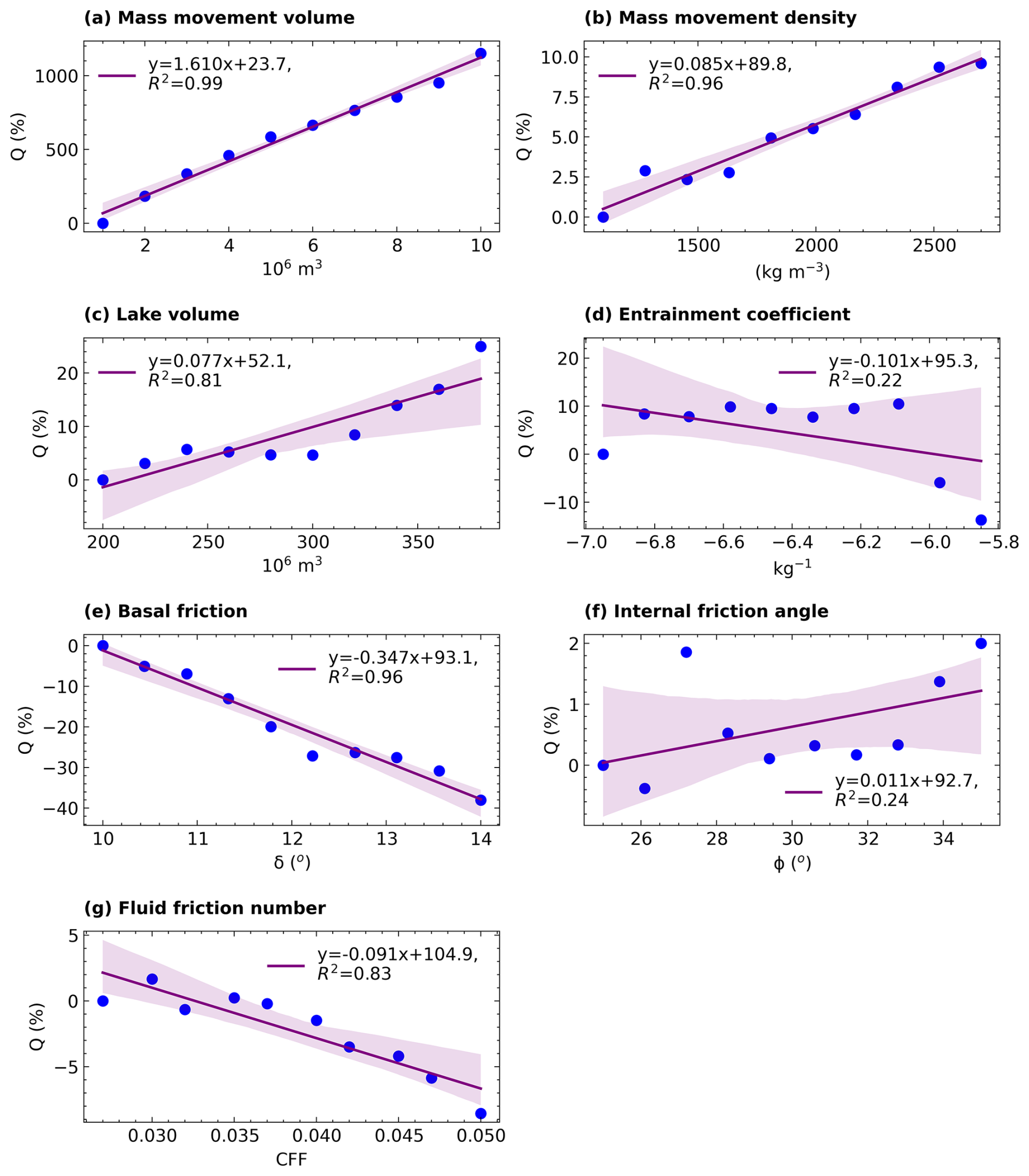
Figure 5 Linear regression between input parameter value variation and percentage change in the resulting peak discharge (Q). The linear regression is computed only for the scalable parameters (a) volume of mass movement entering the lake, (b) mass movement density, (c) volume of the glacial lake, (d) entrainment coefficient, (e) basal friction angle, (f) internal friction angle, and (g) fluid friction number. The shaded envelope around the line shows a 95 % confidence interval.

4.3 Effect of the volume and grain density of mass movement entering the lake

To separate the effect of variation in the volume (V_S) and grain density (ρS) of mass movement entering the lake, we simulated all 10 scenarios of the GLOF event for each volume and density variation using the mass movement initiated from Loc-1. Here we observed that only V_S variation leads to a very large variation in the resulting peak (1160 %) (Fig. 5a) and total discharge (2500 %) (Fig. 6a). Subsequently, this resulted in maximum variation in flow characteristics such as mean flow depth (923 %) and flow arrival time (143 %) (Table 3, Figs. S3–S6). Conversely, the ρS variation showed the least impact on both peak (5 %) and total discharge (24 %) (Figs. 5b, 6b, and 7b) and subsequent characteristics such as flow depth (31 %) and velocity (2 %) (Table 3 and Figs. S3–S6). Both V_S and ρS variation did not result in significant fluctuation in the solid volumetric concentration of the flow (Fig. S3).

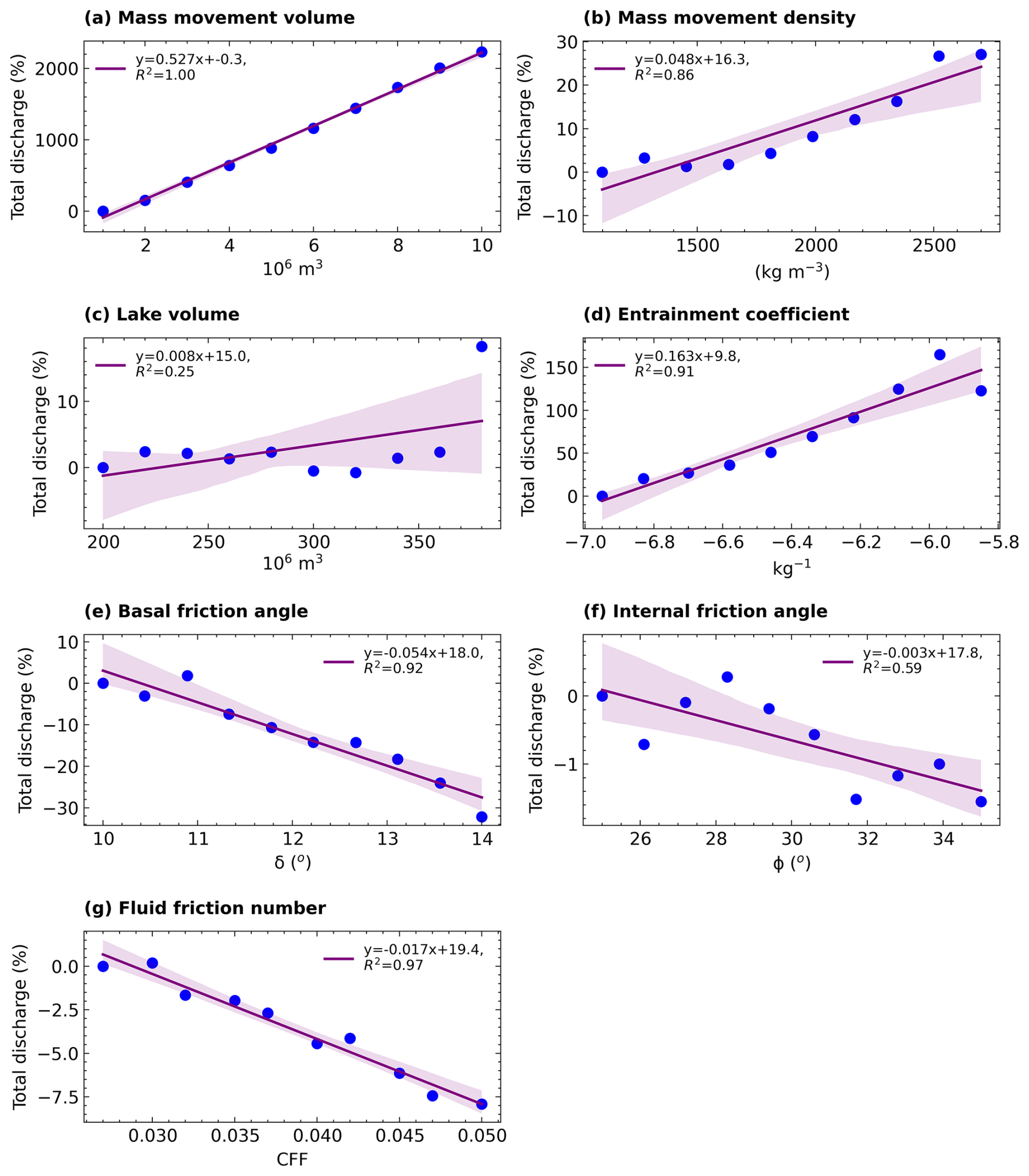
Figure 6 Linear regression between input parameter value variation and the resulting total discharge. The linear regression is computed only for the scalable parameters (a) volume of mass movement entering the lake, (b) mass movement density, (c) volume of the lake, (d) entrainment coefficient, (e) basal friction angle, (f) internal friction angle, and (g) fluid friction number. The shaded envelope around the line shows a 95 % confidence interval.

4.4 Lake volume

Variation in volume of the glacial lake (V_L) from 2 × 10⁸ to 3.8 × 10⁸ m³ results in total peak discharge variations of 25 % with an average of 8.7 % (Fig. 5c). Likewise, the total discharge varied by 18 % with a mean variation of 3 % (Fig. 6c). However, the resulting flow characteristics including flow depth, velocity (Table 3), and arrival time (Fig. 7c) all showed minimal fluctuation, as the total percentage change was well below 10 % (Table 3).

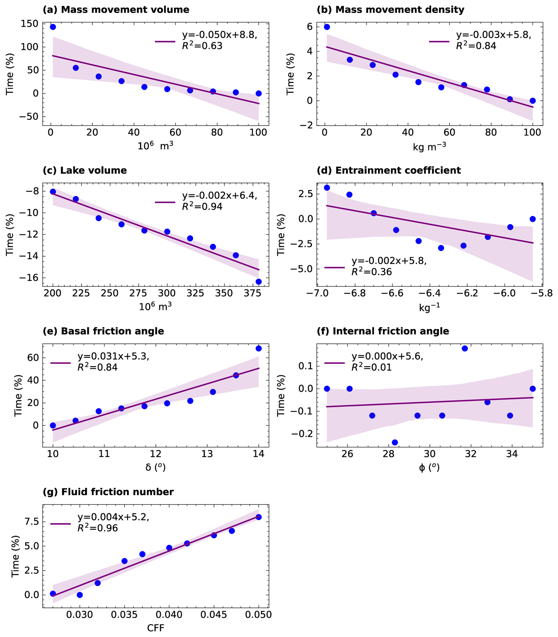
Figure 7 Linear regression between input parameter value variation and flow arrival time. The linear regression is computed only for the scalable parameters (a) volume of mass movement entering the lake, (b) mass movement density, (c) volume of the lake, (d) entrainment coefficient, (e) basal friction angle, (f) internal friction angle, and (g) fluid friction number. The shaded envelope around the line shows a 95 % confidence interval.

4.5 Effect of the entrainment coefficient

Variations in the entrainment coefficient (C_E) substantially impact the resulting GLOF output, causing fluctuations in total discharge by 123 %, although its impact on peak discharge was minimal (13 %) (Figs. 5d and 6d). These changes also affect the flow characteristics including mean depth (49 %) and reach distance (20 %) (Table 3) but had a minimal effect on arrival time (3 %) (Fig. 7d). Interestingly, C_E variation exhibited a threshold effect on peak discharge, total discharge, and flow arrival time. The total discharge increases linearly with increasing C_E up to 10^−5.97 kg⁻¹ but decreases after this. On the other hand, peak discharge increased when C_E increased from 10^−6.95 to 10^−6.83 kg⁻¹, remained constant between 10^−6.83 and 10^−6.09 kg⁻¹, and decreased from there on. The arrival time decreased when the C_E value was increased from 10^−6.46 to 10^−6.46 kg⁻¹ but increased upon a further increase in the C_E value to 10^−5.85 kg⁻¹. Also, unlike other parameters, entrainment variation affected the solid concentration of the flow (Fig. S3). An increase in the entrainment coefficient from 10^−6.95 to 10^−5.85 kg⁻¹ led to a 30 % increase in the mean solid volumetric concentration of the flow.

4.6 Effect of the frictional parameters

Among the frictional parameters, the basal friction angle (δ) resulted in a significant fluctuation in GLOF magnitude (Figs. 5e, 6e, 7e) and subsequent flow characteristics (Figs. S3–S6). While the variation in the fluid friction number (C_FF) had a minimal impact on the resulting peak and total flow (Figs. 5g, 6g), it notably altered other flow characteristics, such as flow velocity (55 %) and depth (70 %) (Table 3). The increase in δ from 10 to 14° resulted in a peak and total discharge decrease of 36 % (Fig. 5d) and 32 % (Fig. 6d), respectively. Likewise, the flow velocity decreased by 23 %, resulting in a delay in flow arrival by 68 % (Table 3). Conversely, the peak flow decreased by 2 % only in response to an increase in the internal friction angle (ϕ) from 25 to 35° (Fig. 5f). The variation in all values of frictional parameters did not result in a significant change in the solid volumetric concentration of the flow (Fig. S5).

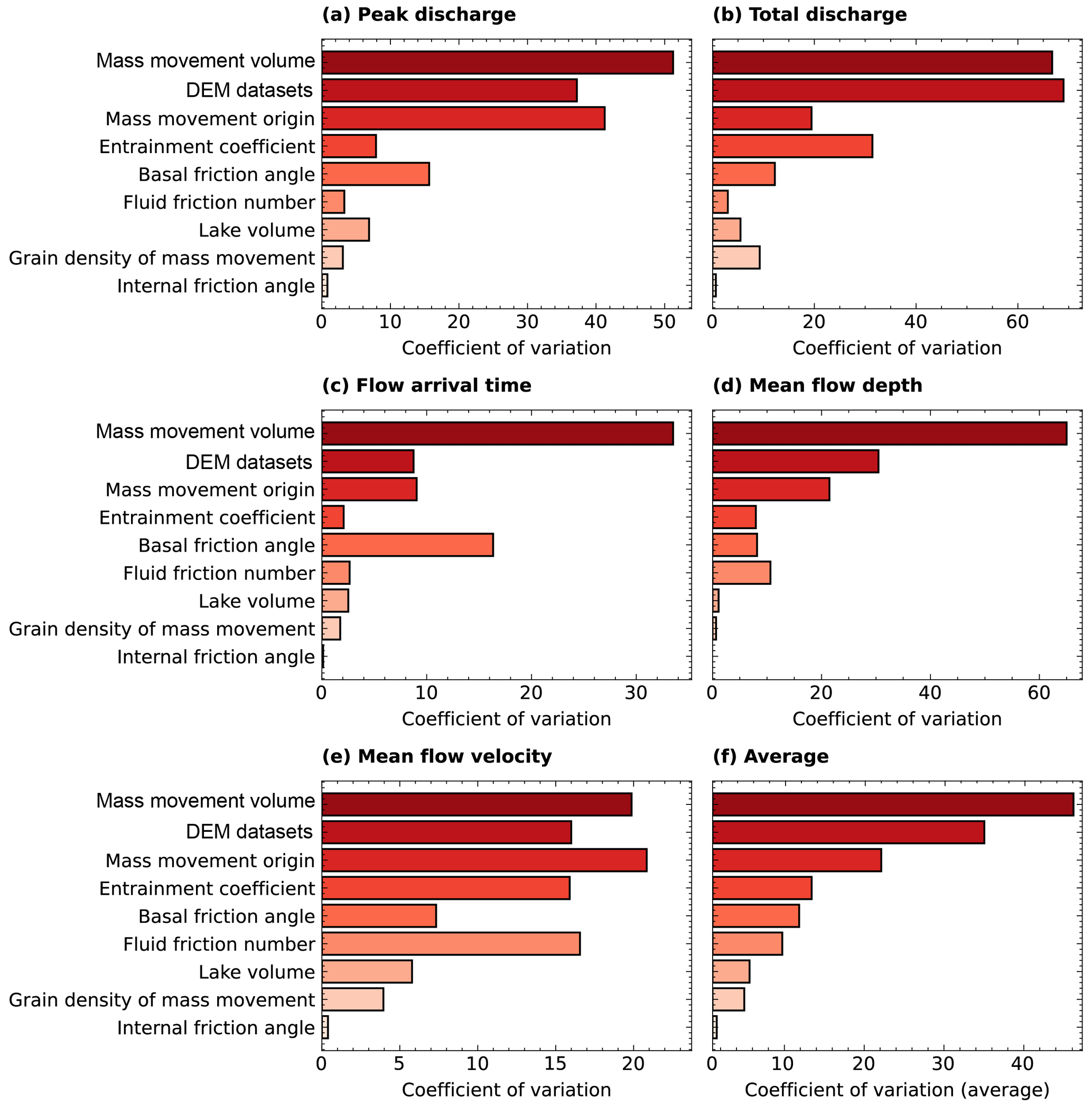
Figure 8 The coefficient of variation for (a) peak flow, (b) volume, (c) time, (d) average flow depth along the river centreline, (e) flow velocity along the river centreline, and (f) average across all these output parameters.

4.7 Comparison of the effects of all parameters

To compare output sensitivity resulting from all input parameters considered here, we calculated the percentage of the coefficient of variation (CV) for peak flow, total discharge, arrival time, flow depth, and flow velocity. We further computed the average CV (avg CV) across all these output variables and examined the overall impact of each input parameter variation (Fig. 8). Comparing all these output indicators, V_S had the greatest impact (avg CV of 47 %), followed by DEM datasets (avg CV of 35 %) and the origin of mass movement (avg CV of 21 %). Other input parameters like δ and C_E also caused significant variation in resulting GLOFs. Notably, C_FF significantly impacted flow depth with its CV of 16 % despite having minimal impact on other flow characteristics (Fig. 8).

For the seven scalable parameters, we computed linear regression (Figs. 5–7). The linear regression analysis revealed that the five parameters: V_S (R²=0.99), ρS (R²=0.96), V_L (R²=0.81), δ (R²=0.96), and C_FF (R²=0.83) demonstrated strong explanatory power in accounting for the variability in GLOF peak discharge (Fig. 5). Among these sets of parameters, V_S (m=1.6), ρS (m=0.085), and V_L (m=0.07) showed a positive relationship, while δ ($m=-\mathrm{0.347}$), C_E ($m=-\mathrm{0.091}$), and C_FF ($m=-\mathrm{0.09}$) exhibited a negative relationship (Fig. 5). All seven parameters (R²>0.86) except for ϕ (R²=0.59) and V_L (R²=0.25) indicated a high level of explanatory power regarding the variation in resulting total discharge (Fig. 6). Comparing all seven input parameters, V_S exhibited the highest R² value for both peak and total discharge, signifying strong explanatory power regarding the modelled flow compared to the other parameters. Additionally, the rate of change in peak discharge and total discharge for every unit increase in V_S was comparatively higher than other parameters as indicated by the steepness of the slope (Figs. 5a and 6a).

Basal friction angle and C_FF demonstrated a high level of explanatory power concerning the variability in flow arrival time, as evidenced by their R² values of 0.98 and 0.97, respectively. V_S variation also exhibited a moderately high explanatory power with a negative relationship, with R² of 0.81 and a slope (m) of −0.019. However, the linearity became less pronounced within the volume range of 4 × 10⁶ to 10 × 10⁶ m³. In contrast, other parameters, including C_E and ϕ, did not exhibit a definitive linear relationship (Fig. 7). However, C_E variation showed a threshold effect on arrival time; increasing C_E from 10^−5.95 to 10^−6.42 kg⁻¹ decreased arrival time, while further increases towards 10^−5.85 kg⁻¹ led to a linear increase in arrival time.

5 Discussion

Our primary aim was to investigate the sensitivity of the modelled GLOF outputs to a range of values for key model input parameters using the r.avaflow model. Previous studies have underscored the sensitivity of GLOF model outputs to some input parameters, including the basal friction angle, entrainment coefficient, and volume of mass movement entering the lake (Baggio et al., 2021; Mergili et al., 2018b, 2020a). This study advances our understanding of GLOF modelling by conducting a comprehensive sensitivity analysis across nine essential parameters and multiple (84) GLOF simulations. As a result, we have, for the first time, ranked these nine GLOF input parameters based on their contributions to model output variabilities. Our results showed that modelled GLOF output parameters are substantially sensitive to five of the nine parameters we tested here (DEM dataset, volume of mass movement entering the lake, origin of mass movement entering the lake, entrainment coefficient, and basal friction angle), suggesting that GLOF modelling results are subject to uncertainty from multiple sources. The findings offer valuable perspectives on the uncertainty in GLOF modelling results and complexities inherent in modelling the GLOF process chain within rugged mountain terrain such as in the Himalaya.

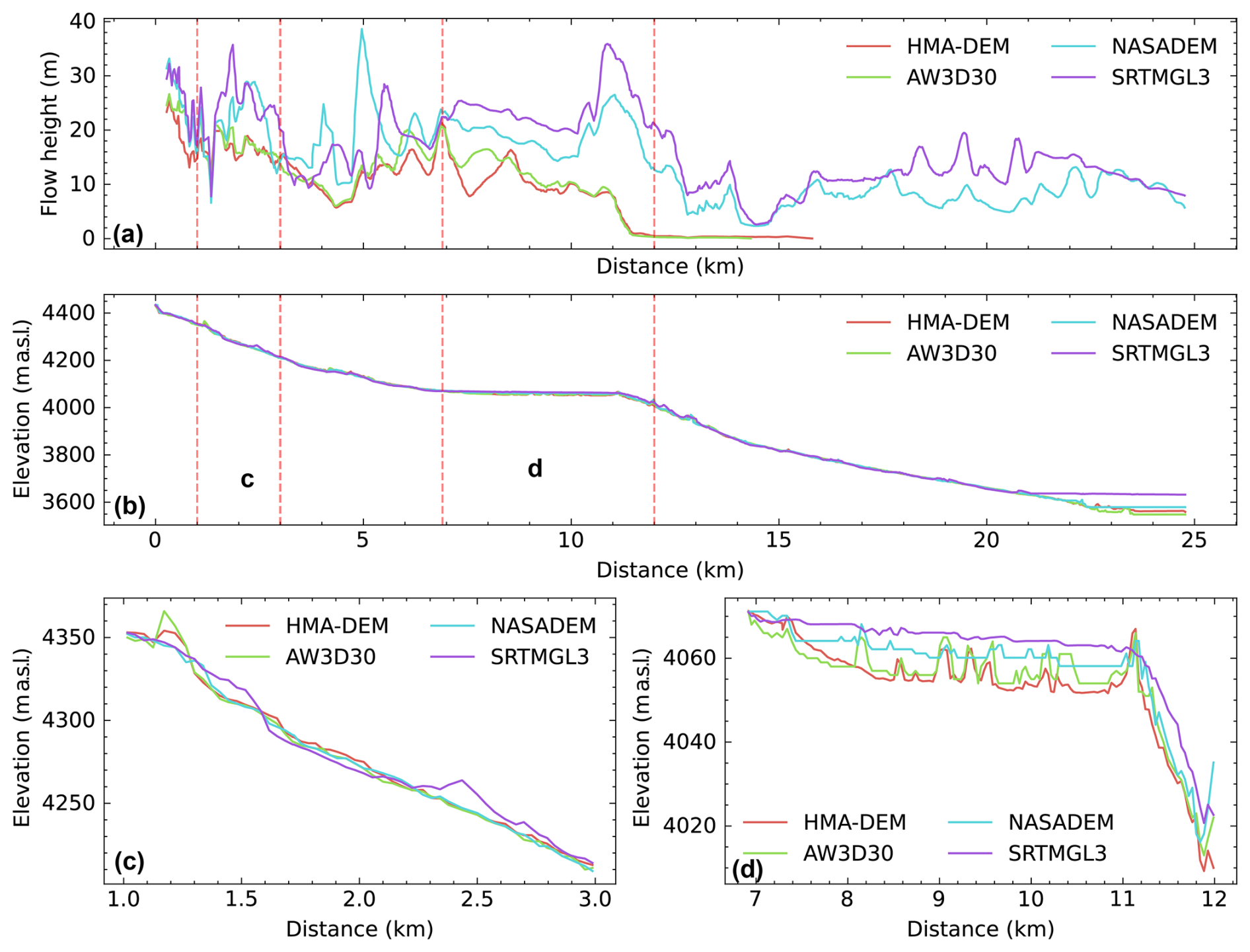
Figure 9 A comparison of the elevation profiles from four DEM datasets and the corresponding flow depths along the river centreline, generated through r.avaflow modelling. Panels (a) and (b) show the flow depths and elevation profiles along the river centreline. Panels (c) and (d) illustrate elevation profiles for two specific sections marked in (a) and (b). DEM and flow depth profiles from the vertical cross-sections at various distances are also provided in the Supplement (Fig. S7). The DEM datasets were co-registered using the algorithm developed by Shean et al. (2016).

5.1 DEM datasets

A DEM is one essential piece of data for modelling GLOFs and other types of floods (Hawker et al., 2018; Saksena and Merwade, 2015; Schumann and Bates, 2018; Westoby et al., 2014). The impact of DEM resolution is even more pronounced in the steep and complex topographic conditions prevalent in high-mountain regions like the Himalaya (Liu et al., 2019). Our study provides the quantification of the effect of DEM in such environments for the first time. Our results suggest that the use of global and regional DEM datasets with a resolution ranging from 8 m (HMA-DEM) to 90 m (SRTMGL3) leads to over 2-fold and 4-fold variations in peak and total discharge, respectively, and causes successive significant fluctuations in flood height, reach distance, and flow arrival time. This likely results from the low-resolution DEMs not fully resolving the river channel compared to higher-resolution DEMs. This limitation results in a reduction in surface roughness and river channel conveyance (carrying capacity of channel). Thus, the flow spreads out more, leading to an increase in the modelled flow extent and reach (Figs. 9 and S7) (Muthusamy et al., 2021). This was supported by comparing the DEM profile and flow depth along the river centreline (Fig. 9) and across the multiple vertical cross-sections along the river channel (Fig. S7). The analysis showed that GLOF output from SRTMGL3, where river channels are poorly resolved, was comparatively higher than that from HMA-DEM with the better-resolved channel. Also, DEM datasets were acquired at different times, meaning the topographic features they captured will also differ depending on natural geomorphological change or human-made alteration of the earth's surface over time (Khosh Bin Ghomash et al., 2019; Bishop et al., 2002; Schumann and Bates, 2018; Watson et al., 2015). Such discrepancies will have a substantial influence on flow characteristics and uncertainty if a DEM with inadequate spatial and temporal resolution is used in GLOF modelling.

Overestimation of flood maps stemming from reductions in DEM resolution has been reported in urban flood modelling (Muthusamy et al., 2021; McClean et al., 2020). However, the impact of DEM data on GLOF modelling, especially in a complex topographic setting such as in the Himalaya, has been rarely documented (Wang et al., 2011). Our results show the substantial variation in GLOF model output stemming from DEM dataset variation, even when employing DEMs with comparable spatial resolutions, underscoring the criticality of high-quality DEM data in GLOF modelling (Fig. 9). DEM datasets covering rugged high-mountain terrain, where GLOFs typically occur, are likely to have more errors due to geometric distortion and data loss due to challenges involved in data acquisition for DEM production (Hugonnet et al., 2021; Liu et al., 2019). Therefore, using global- to regional-scale open-access DEMs, such as SRTM for GLOF modelling, due to the absence of high-resolution alternatives (Wang et al., 2011) may only be suitable for a first-order assessment of GLOFs at large scales (Zhang et al., 2023b). This is important as uncertainty stemming from DEM datasets is often overlooked and/or not well addressed in the previous basin-specific GLOF modelling work (Rinzin et al., 2023; Sattar et al., 2023, 2021b).

5.2 Variation in the origin of mass movement

Our study indicated that different origins of mass movement initiation produced GLOFs with approximately 2-fold variations in their peak discharge, volume, and reach distance (Fig. 4). These variations can be explained based on the lake geometry and the direction, horizontal distance, and vertical distance at which the mass movement enters the lake. The r.avaflow model provides detailed output parameters such as kinetic energy associated with the flow and a flow depth map for each time step, which allowed us to better understand the cause of this variation. For example, the mass movement originating from Loc-1, which is located at the slope above the headwall, directly impacts the head end of the lake with the highest kinetic energy (50 714 GJ) of all sources of mass movement. This head-end impact, coupled with its high energy, facilitates the direct forward propagation of waves toward the frontal outlet, causing the lake water to overtop the frontal moraine and resulting in a higher peak and total discharge (Fig. S8). Thorthormi Tsho is roughly crescentic in shape and curves toward the west, with its maximum curvature facing the origin of mass movement of Loc-5. This shape also allows for the impact wave generated from mass movement from Loc-5 to move almost unimpeded along the flow line, resulting in greater GLOF discharge. Also, Loc-1 and Loc-5 are located at greater distances and higher elevations from the lake compared to other locations (Fig. 2). This spatial location might have also enabled them to generate greater force to impact the lake. In contrast, the direct wave of impact generated by the mass movement from Loc-3, located on the slope above the right moraine dam, is deflected towards the left lateral moraine and only a secondary wave proceeds towards the lake outlet, resulting in a comparatively lower peak and total discharge (Fig. S8) (Emmer et al., 2024). This finding implies that the geometry of the glacial lake and the surrounding source slope plays a vital role in GLOF output. Thus, we underscore the importance of considering catchment shape in GLOF modelling, although we cannot assume that two identical basins will have the same flood properties due to the influence of other factors, such as the involved volume of solid and fluid parts.

Earlier studies (Mergili et al., 2017, 2020b) have explained the interaction between landslides and reservoirs (lakes) and their influence on the resulting hydrograph. However, these studies did not consider the variables such as directions and distances from which the mass impacts the lake. To fill this gap, here we enhanced our understanding of the interplay between the resulting GLOF magnitude and mass movement attributes including the direction and distance from which the mass enters the lake, the amount of kinetic energy the mass possesses, and the geometry of the lake. Our results emphasize the significant impact on the resulting GLOF events caused by the uncertainty in pinpointing the specific location of the origin of mass movement entering the lake. The thawing of permafrost and destabilization of the slope surrounding the lake due to climate warming (Gruber et al., 2017; Kääb et al., 2018; Sattar et al., 2025) combined with the expansion of the glacial lake towards the mountain flank (Rounce et al., 2016) are likely to increase the frequency of mass movement entering the lake, further exacerbating this uncertainty. By effectively identifying and quantifying the uncertainties related to the origin of mass movement entering the lake in addition to the volume, we propose considering the origins of mass movement in designing the scenario-based GLOF modelling in future studies. This approach goes beyond the existing practice, which primarily focuses on the volume of mass movement entering the lake. This is important because, as demonstrated in our study, the impact of mass movement can vary significantly depending on its origin. In some cases, what may be considered a worst-case scenario from one origin might represent only a low-magnitude event from another (GAPHAZ, 2017; Sattar et al., 2021a; Allen et al., 2022).

5.3 Mass movement volume, grain density, entrainment coefficient, and lake volume

Our investigation revealed that variation in GLOF magnitude is most sensitive to the volume of mass movement (V_S) entering the lake. It also exhibits a significant level of sensitivity to the entrainment coefficient (C_E), whilst the grain density (ρS) and lake volume (V_L) exhibit a negligible impact. For example, the variation in V_S between 1×10⁶ and 10×10⁶ m³ leads to peak and total discharge fluctuation of 1160 % and 2500 %, respectively, and subsequent variation in maximum flow depth and arrival time (Figs. 5 to 7). The dominant impact of V_S and C_E on GLOF magnitude could be due to their direct influence on the overall magnitude and intensity of flood events. The total discharge during the GLOF cascade event is a function of V_S entering the lake. This is further corroborated by the near-perfect linear relationship of peak discharge (R²=0.99) and total discharge (R²=1) with V_S entering the lake observed here. Likewise, the volume of solid content in the flow is solely contributed by the entrainment of frontal moraine material, primarily determined by C_E. Additionally, this correlation could be attributed to the amount of energy and associated momentum of the flow, which increases significantly with a corresponding increase in V_S. Also, it could be due to the longer timing and duration of the flow as evident in Fig. S2. Most GLOF events in high mountains across HMA and other alpine regions are caused by moraine dam breaches triggered by mass movement entering the lake from the surrounding mountain flank (Shrestha et al., 2023; Lützow et al., 2023; Emmer and Vilímek, 2014). As a result, V_S is considered a primary basis for scenario development (Allen et al., 2022). Thus, we believe this finding provides useful insights for improving the development of different scenarios of GLOFs with higher confidence or is a basis for ensemble testing, with the caveat that the range of outputs may be too wide to be of practical use.

The volume of a glacial lake is one of the key parameters in GLOF modelling and subsequent hazard mapping. Without field-measured bathymetry, we applied eight different empirical equations to estimate the volume of Thorthormi Tsho, which ranged between 2.1 × 10⁸ and 3.80 × 10⁸ m³. Interestingly, this variation in V_L did not significantly influence the modelled GLOF hydraulics; V_L was ranked as the third least sensitive parameter in our analysis. This limited impact may be attributed to the large size of Thorthormi Tsho (∼ 4.35 km³) and its substantial storage capacity, as estimated by the empirical equations used for calculating lake volume here. Even the lower bound of the calculated V_L exceeds 95 % of the measured volume of the glacial lake, and the upper bound is greater than 58 of the 59 measured lake volumes in the greater Himalaya (Zhang et al., 2023a). We believe that Thorthormi Tsho's large volume and expansive area enable it to absorb and dissipate the energy from potential mass movement impacts, effectively acting as a buffer (Emmer et al., 2024). Nevertheless, while our findings suggest that V_L uncertainty may have a relatively minor impact on GLOF modelling for large lakes like Thorthormi Tsho, we acknowledge that V_L remains a critical parameter in GLOF modelling, particularly for smaller lakes where volume changes could have a more pronounced effect on flood dynamics (Sattar et al., 2023).

5.4 Variations in frictional parameters

Among the frictional parameters, our result showed that GLOF magnitude is most sensitive to the basal friction angle (δ). For example, the variation in total discharge (47.5 %) resulting from fluctuation in δ within the experiment range was 30 times greater than that of the internal friction angle (ϕ) and over 4 times greater than that of the fluid friction angle (C_FF). δ plays a dominant role in flow dynamics and the interaction between the flowing material and the channel bed. This direct contact means that even minor changes in δ can have substantial effects on the resistance encountered by the flowing material, thereby influencing the mobility of the flow (Pudasaini and Krautblatter, 2014a; Mergili et al., 2018a, b). ϕ on the other hand primarily affects particle interactions within the flowing material, whilst C_FF is a coefficient which quantifies the overall flow resistance within the flow path, mainly depending on surface roughness. Our findings indicate that prioritizing the consideration of δ over the other two frictional parameters is advisable. While the back-calculated values might seem to be reasonable initiation values for δ as measuring it in the field is practically not feasible, we recommend conducting a statistically substantial sensitivity analysis using adequate sampling size and an appropriate statistical model. Despite the relatively low overall impact on GLOF magnitude, C_FF notably increased the flow's mobility, especially beyond 12 km downstream, when the flow became fluid-dominant (Fig. S4). This is because C_FF controls the mobility of the fluid part (Mergili and Pudasaini, 2024; Mergili et al., 2017). This suggests that C_FF could exert a substantial influence, particularly in modelling scenarios encompassing longer flow distances.

5.5 Key points from the comparison of all parameters and the way forward

Identifying the most accurate parameter values or optimal datasets can be achieved through validation with well-constrained historical events (Zheng et al., 2021a; Schneider et al., 2014; Mergili et al., 2020b; Shugar et al., 2021; Sattar et al., 2025), but there are limitations in the transferability of these findings due to unique characteristics and initial conditions of each GLOF, such as varying proportions of solid and liquid parts. Because of this we effectively constrained how variation in input parameter values within commonly used ranges influences the GLOF modelling results, instead of trying to determine the correct value for each parameter. Or, put another way, if we apply our study to a specific example, we may determine that certain factors are more important than others for this specific example, but it would be unclear how applicable our results are to other events. Thus, we see our approach as the least biased towards any event and hence the most generally applicable approach. Our results indicating modelled GLOFs being subjected to uncertainty from multiple input parameters implies that the parameter value determined from one modelled GLOF event might not accurately predict the behaviour of GLOFs in different regions or under different circumstances (Mergili et al., 2018a, 2020b). Therefore, while these back-analysed parameter values can provide valuable insights, they need to be applied with caution and adapted to the specific context of each new GLOF scenario. As a result of these multiple sources of uncertainty in modelled GLOFs, it could pose challenges in effectively communicating risks with communities and other stakeholders (Thompson et al., 2020). We highlight that more sensitive parameters should be treated carefully in future GLOF modelling works by robustly considering associated uncertainties.

Due to the high sensitivity of the model output on DEM resolution, we emphasize the critical importance of a high-resolution and good-quality DEM (Uuemaa et al., 2020; Schumann and Bates, 2018), especially when modelling is aimed at producing hazard maps with higher granularity at the specific basin scale. DEMs should have a high spatial resolution, have a high vertical accuracy, and be recently produced, especially in areas of high relief and rapid landscape change such as in the Himalaya (Schumann and Bates, 2018). Previous studies have indicated that flood modelling accuracy can be improved by addressing the effect of DEM resolution and accuracy (Saksena and Merwade, 2015) or by merging with other high-resolution and accurate DEMs (Muthusamy et al., 2021). These methods appear viable in the context of highly sparse coverage of high-resolution DEMs and the unaffordability of high-resolution commercial DEMs, but the modelling results may be subjected to substantial uncertainty.

The mass movement volume and δ exhibit a strong linear relationship with all output parameters. Whilst the linear relationship does not negate the influence these parameters have on flow characteristics, it suggests that model output errors resulting from uncertainties in these parameters might be predictable. This is essential since predicting the V_S movement involved in the forward modelling is highly challenging and determining an accurate value is impossible – the current challenge is rather to establish a likely envelope of volumes. However, such a prediction should be bespoke to the particular events based on the initial parameters like estimated ice thickness, slope, and the presence of permafrost. Furthermore, such predictions must also consider other factors, such as equifinality arising from the interaction of multiple parameters (Mergili et al., 2018a, b, 2020b).

The entrainment coefficient exhibits a threshold effect for peak discharge, arrival time, and total discharge, but these thresholds occur at different C_E values for each of these output parameters. The observed threshold effects in flow characteristics can likely be attributed to the initial dominance of the fluid component, wherein the contribution of erosion to the flow dynamics is negligible. As the erosion rate progresses with increasing C_E values, the increasing concentration of eroded material reduces the mobility of the flow, leading to a decline in mobility of the flow. These threshold effects suggest that once these thresholds are surpassed, the resulting flow and arrival time demonstrate a heightened sensitivity to variations in entrainment. Consequently, this sensitivity may translate to the flow characteristics such as flow depth and arrival time which are essential for hazard and risk assessments. It is important to note that this threshold value may vary across different GLOF events due to the diverse combinations of other parameters.

The GLOF simulations were conducted using the r.avaflow model due to its capability to model the entire GLOF process chain (Mergili and Pudasaini, 2024; Mergili et al., 2017). While we present the uncertainty involved in the full GLOF process chain from mass movement entering the lake to downstream propagation, we specifically explored the uncertainty in the GLOF input parameters relevant to r.avaflow modelling. Input parameters such as DEM datasets and the volume and density of mass movement involved in a GLOF event might be similar across different models. However, it should be noted that all parameters tested here do not necessarily apply to all models used for GLOF modelling.

The flow arrival time was measured from the profile located 3, 6, and 9 km downstream of the lake since some of our modelled GLOF terminates before proceeding further downstream. This is a reasonable point as human settlement downstream of the lake is mostly concentrated around this area. The variation in flow arrival time might be underestimated if the location is farther downstream from the lake.

Here we focused on nine essential parameters in r.avaflow, which are relevant to GLOF modelling. As an open-source modelling code, the r.avaflow model offers flexibility by allowing the users to manipulate all parameters, a level of transparency that sets it apart from many modelling codes. However, including inbuilt modules, initial conditions, and all flow parameters, r.avaflow has more than 30 tuneable parameters (Mergili and Pudasaini, 2024) (Table S1). Our choice of parameter in this study is essentially motivated by those identified as critical and commonly modified in the previous GLOF modelling studies and which are frequently modified to fit with the parameter from back-calculated events. Because of this, our sensitivity analysis might have potentially overlooked the complexity of r.avaflow stemming from the effect of all these parameters, let alone their interaction effect. Also due to the enormous computational time and resources required for running r.avaflow, we used one-at-a-time sensitivity analysis conducting up to 10 simulations per parameter. While this number of simulations for each parameter produced substantially conclusive results, we do not discount the robustness of the global sensitivity analysis employing an adequate sampling size which can adequately account for the influence of parameter interactions (Saltelli et al., 2004). While we consider for the first time the importance of the uncertainty in these parameters in GLOF modelling, in the light of all these limitations, we provide the following recommendations. (1) We recommend that future studies include a broader range of parameters, further advancing the understanding of their roles in GLOF modelling. (2) This can be achieved by initially focusing on the most sensitive parameters identified in this study and progressively expanding the analysis to include other parameters. Adequate sample sizes and appropriate statistical models should be employed to ensure robust findings. (3) Given that r.avaflow is an open-source tool under continuous development, we underscore the implementation of features that support parallel computation for parameter interaction analyses. This advancement would enable future studies to fully utilize high-performance computing (HPC) resources and address complex modelling challenges more effectively.

6 Conclusions

GLOFs present substantial dangers to communities residing in valleys downstream of glacial lakes. GLOFs involve complex cascading processes and typically occur across rugged mountain terrains. Due to these complexities, modelling GLOFs necessitates extensive input data, parameters, and complex modelling codes for accurate hazard and risk assessments, which is inherently challenging. However, previous studies have mostly relied on open-access data and are grounded in a historical event introducing significant uncertainties to the modelling results. In this study, we have, for the first time, conducted a sensitivity analysis considering multiple GLOF parameters and ranked these inputs based on how their uncertainties in input values apportion to the variation in modelling output by employing cutting-edge modelling code, r.avaflow. Our results suggested GLOF modelling outputs such as peak and total discharge are substantially sensitive to variation in input values of six out of nine parameters we tested here. Specifically, the modelling outputs are the most sensitive to the volume of mass movement entering the lake followed by the variation in DEM datasets and the location of the origin of mass movement entering the lake. Other parameters like the basal friction angle and entrainment coefficient also showed significant sensitivity. Although limited to GLOF modelling with the r.avaflow model, our study emphasizes that GLOF modelling results are influenced by uncertainties stemming from various sources, underscoring the need for careful interpretation of the modelling results. By ranking the model parameters according to their impact on model output, our study prioritizes model input parameters for future modelling efforts, given the challenge of adequately constraining multiple parameters. Additionally, this study lays the groundwork for a thorough investigation into the most sensitive parameters to improve our understanding of GLOF modelling.