Global application of a regional frequency analysis to extreme sea levels

Coastal regions face increasing threats from rising sea levels and extreme weather events, highlighting the urgent need for accurate assessments of coastal flood risk. This study presents a novel approach to estimating global extreme sea level (ESL) exceedance probabilities using a regional frequency analysis (RFA) approach. The research combines observed and modelled hindcast data to produce a high-resolution (∼1 km) dataset of ESL exceedance probabilities, including wave setup, along the entire global coastline (excluding Antarctica).

The methodology presented in this paper is an extension of the regional framework of Sweet et al. (2022), with innovations introduced to incorporate wave setup and apply the method globally. Water level records from tide gauges and a global reanalysis of tide and surge levels are integrated with a global ocean wave reanalysis. Subsequently, these data are regionalised, normalised, and aggregated and then fit with a generalised Pareto distribution. The regional distributions are downscaled to the local scale using the tidal range at every location along the global coastline obtained from a global tide model. The results show 8 cm of positive bias at the 1-in-10-year return level when compared to individual tide gauges.

The RFA approach offers several advantages over traditional methods, particularly in regions with limited observational data. It overcomes the challenge of short and incomplete observational records by substituting long historical records with a collection of shorter but spatially distributed records. These spatially distributed data not only retain the volume of information but also address the issue of sparse tide gauge coverage in less populated areas and developing nations. The RFA process is illustrated using Cyclone Yasi (2011) as a case study, demonstrating how the approach can improve the characterisation of ESLs in regions prone to tropical cyclone activity. In conclusion, this study provides a valuable resource for quantifying the global coastal flood risk, offering an innovative global methodology that can contribute to preparing for – and mitigating against – coastal flooding.

1 Introduction

Flooding represents one of the greatest threats to coastal communities globally, with devastating impacts for affected regions. Notable events which have caused significant coastal flooding in recent years include Cyclone Amphan (2020), which struck the Bay of Bengal and produced a storm surge of up to 4.6 m along the coast of West Bengal, killing 84 people and causing total losses of over USD 13 billion (India Meteorological Department, 2020; Kumar et al., 2021); Hurricane Harvey (2017), the second most costly hurricane to hit the US after Katrina (2005), which impacted 13 million people and hit the state of Texas with a maximum storm surge of 3.8 m (Amadeo, 2019); and Typhoon Jebi (2018), driving storm surges of over 3 m in Osaka Bay, Japan, combined with wave action which led to flooding exceeding 5 m above mean sea level (Mori et al., 2019). Approximately 10 % of the world's population (768 million people) lives below 10 m above mean sea level (McGranahan et al., 2007; Nicholls et al., 2021). Coastal flooding is expected to increase dramatically in the future, predominantly caused by sea level rise (Calafat et al., 2022; Taherkhani et al., 2020) and compounded by continued growth and development in coastal populations (Neumann et al., 2015). Therefore, continuing to improve the understanding of coastal flooding is vital.

Coastal floods are driven by extreme sea levels, which arise as combinations of (1) astronomical tides; (2) storm surges (driven by tropical and extratropical cyclones) and associated seiches; (3) waves, especially setup and runup; and (4) relative mean sea level changes (including sea level rise and vertical land movement). Risk assessments of coastal flooding require high-quality and high-resolution flood hazard data, typically in the form of flood inundation maps. Inundation maps are usually derived from hydraulic models, which use high-resolution extreme sea level (ESL) exceedance probabilities as a key input (e.g. Bates et al., 2021; Mitchell et al., 2022). The development of coastal inundation maps is reliant on coastal boundary condition points that vary in resolution depending on the application. Previous studies (e.g. Barnard et al., 2019) have used 100 m resolution at local scales, while regional studies (e.g. Bates et al., 2021; Environment Agency, 2018) have employed resolutions between 500 m and 2 km.

Traditional methods for computing ESL exceedance probabilities involve extreme-value analysis of measurements from individual tide gauges or wave buoys. However, long complete records spanning numerous decades are necessary to obtain robust estimates of ESL return levels (Coles, 2001). The Global Extreme Sea Level Analysis (GESLA-3) database provides sea level records for over 5000 tide gauge stations (Haigh et al., 2021), but these tide gauges still cover only a small fraction of the world's coastlines. Wave buoys are even more sparse, largely restricted to the Northern Hemisphere, and long historical records are marred by discontinuities (Timmermans et al., 2020). Even in areas with relatively high tide gauge or wave buoy density, there are still large expanses of coastline which remain ungauged. While rare extreme weather events (such as intense tropical cyclones – TCs) are often many hundreds of kilometres in size, the precise impact of the corresponding ESL can often be highly localised (Irish et al., 2008), meaning that the peak surge occurs at an ungauged location. The particular locale of peak surge for an event is determined by storm characteristics, local bathymetry, and coastal geography, amongst other factors (Shaji et al., 2014). Therefore, relying on past observation-based analyses of ESL exceedance probabilities to characterise return levels across a region will likely lead to underrepresentation of rare extreme events. Finally, another limitation is that many previous analyses of ESL exceedance probabilities consider the still-water-level component (i.e. tide plus storm surge) separately from the wave setup and runup (Haigh et al., 2016; Muis et al., 2016; Ramakrishnan et al., 2022).

One solution to overcome sparse datasets is to use ESL hindcasts created by state-of-the-art models. These include regional (e.g. Andrée et al., 2021; Siahsarani et al., 2021; Tanim and Akter, 2019) or global tide–surge (such as Deltares' Global Tide and Surge Model v3.0, hereafter referred to as GTSM; Muis et al., 2020) or wave models (e.g. Liang et al., 2019). These are used to fill the spatial and temporal gaps in the observation records via historical reanalysis simulation. However, their ability to accurately capture extreme events is hampered by the atmospheric forcing data that are used to drive the models, as reanalysis products like ERA5 (Hersbach et al., 2020) commonly contain biases in representing meteorological extremes such as TCs (Slocum et al., 2022), leading to an underestimation of event intensity. Furthermore, the time period captured in reanalysis products is not adequate to represent the characteristics (e.g. frequencies) of particularly rare events such as intense TCs. To overcome this limitation, some studies have used synthetic event datasets representing TC activity over many thousands of years (e.g. Dullaart et al., 2021; Haigh et al., 2014); however, this approach is computationally expensive.

An alternative and less computationally demanding solution that helps to address some of the problems inherent to estimating ESLs around the world's coastlines from the observational record is regional frequency analysis (RFA). The RFA methodology was originally developed to estimate streamflow within a hydrological context (e.g. Hosking and Wallis, 1997) but has since been used in many applications requiring extreme-value analysis of meteorological parameters including coastal storm surge (e.g. Arns et al., 2015; Bardet et al., 2011; Weiss and Bernardara, 2013) and extreme ocean waves (e.g. Campos et al., 2019; Lucas et al., 2017; Vanem, 2017). The principle of RFA is founded on the basis that a homogenous region can be identified throughout which similar meteorological forcings and resultant storm surge or wave events could occur, even if the extreme events have not been seen in part of that region in the historical record (Hosking and Wallis, 1997). RFA has been used on a regional scale to produce coastal ESL exceedance probabilities, e.g. in France (Andreevsky et al., 2020; Hamdi et al., 2016), on the US coastline (Sweet et al., 2022), in northern Europe (Frau et al., 2018), at US coastal military sites (Hall et al., 2016), and in the Pacific Basin (Sweet et al., 2020). However, an RFA approach has not (to our knowledge) been applied globally.

The overall aim of this paper is to apply, for the first time, an RFA approach to estimate ESL exceedance probabilities, including wave setup, along the entire global coastline. These exceedance probabilities aim to better characterise ESLs driven by rare extreme events, such as those from TCs, which are poorly represented in the historical record. Uniquely, this study uses both measured and hindcast datasets; includes tides, storm surges, and wave setup; and calculates exceedance probabilities at high resolution (1 km) globally. The specific objectives of this paper are

1. to develop and apply RFA globally (excluding Antarctica) utilising both observational tide gauge and modelled hindcast sea level and wave records;

2. to illustrate how the RFA methodology improves the representation of rare extreme events in the ESL exceedance probabilities using Cyclone Yasi, which impacted the Australian coastline in 2011, as a case study;

3. to validate the RFA against exceedance probabilities estimated from the GESLA-3 global tide gauge database; and

4. finally, to quantify how much the RFA increases the estimation of ESL exceedance probabilities in areas prone to TC activity when compared to single-site analysis using hindcast datasets (Muis et al., 2020; Dullaart et al., 2021).

This paper is laid out as follows: the datasets used are described in Sect. 2. The methodology is detailed in Sect. 3, addressing objective 1. The results and validation are described in Sect. 4, addressing objectives 2, 3, and 4. A discussion of the key findings and conclusions are then given in Sects. 5 and 6, respectively.

2 Data

We use seven primary sources of data in this study: (1) still-water sea level observations contained in the GESLA-3 tide gauge dataset, (2) global still-water sea level simulations from the GTSM hindcast based on the ERA5 climate reanalysis, (3) tidal predictions from the FES2014 finite-element hydrodynamic model, (4) significant wave heights derived from the ERA5 climate reanalysis, (5) mean dynamic topography from HYBRID-CNES-CLS18-CMEMS2020, (6) a Copernicus digital elevation model (DEM) to create a global coastline dataset, and (7) the COAST-RP dataset from (Dullaart et al., 2021) to validate the RFA methodology. These seven datasets are described below.

Still-water sea level records are assembled from the GESLA-3 (Global Extreme Sea Level Analysis) tide gauge dataset version 3 (Caldwell et al., 2015; Haigh et al., 2021). The GESLA-3 dataset includes high-frequency water level time series from over 5000 tide gauges around the globe, collated from 36 international and national providers. Data providers have differing methods of quality control; however, each record was visually assessed by the authors of the GESLA-3 dataset and graded as having either (i) no obvious issues, (ii) possible datum issues, (iii) possible quality control issues, or (iv) possible datum and quality control issues. Only records with no obvious issues were used in this study.

As discussed in Sect. 3, the GTSM-ERA5 hindcast dataset is used in all areas which are not covered by tide gauge observations. GTSM is a depth-averaged hydrodynamic model built using the DELFT-3D hydrodynamic model, which makes use of an unstructured global flexible mesh with no open boundaries (Muis et al., 2020). The model has a coastal resolution of 2.5 km (1.25 km in Europe) and a deep-ocean resolution of 25 km. The GTSM-ERA5 dataset spans the period from 1979 to 2018 and was developed by forcing GTSM with hourly fields of ERA5 wind speed and atmospheric pressure at 10 m (Hersbach et al., 2020). GTSM-ERA5 has a 10 min temporal resolution and provides a times series at locations approximately every 50 km along the coastline (10 km in Europe). Validation carried out by Muis et al. (2020) shows that the dataset performs well against observations of annual maximum water level, exhibiting a mean bias of −0.04 m and a mean absolute percentage error of 14 %.

We use the FES2014 tidal database to generate tidal time series at GTSM-ERA5 locations and RFA output locations. The RFA output resolution is much higher than the output resolution of GTSM-ERA5, which is why FES2014 is used instead. FES2014 is a finite-element hydrodynamic model which combines data assimilation from satellite altimetry and tide gauges (Lyard et al., 2021). The model solves the barotropic tidal equations as well as the effects of self-attraction and loading. The gridded resolution of the output is $\mathrm{1}/\mathrm{16}$°. The model was extensively validated against tide gauges, satellite altimeter observations, and alternative global tide models by Lyard et al. (2021) and was found to have an improved variance reduction in nearly all areas, especially in shallow-water regions. The Python package distributed with the FES2014 data (https://github.com/CNES/aviso-fes, last access: February 2022) was used to simulate tidal time series.

To calculate wave setup we use significant wave heights (H_s) from the ERA5 reanalysis (Hersbach et al., 2020) covering the period from 1979 to 2020. The spatial resolution of the ERA5 wave model output is 0.5° by 0.5° and the temporal resolution is hourly. Independent validation of hourly H_s performed by Wang and Wang (2022) finds little bias in the dataset (−0.058 m); however, the authors go on to conclude that H_s of extreme waves tends to be underestimated (by 7.7 % in the 95 % percentile), a conclusion supported by Fanti et al. (2023).

We use mean dynamic topography (MDT) to convert water levels from mean sea level as measured by tide gauges to mean sea level as referenced by a geoid for use in subsequent studies involving inundation assessments using hydraulic modelling. MDT describes the change in sea surface height due to the effects of winds and currents in the ocean. Digital elevation models (DEMs), a key input to hydraulic models, typically use a geoid as a vertical datum. A geoid is an equipotential surface of mean sea level under the sole effect of gravity in the absence of land masses, currents, and tides (Bingham and Haines, 2006). To convert water levels from the tide gauge mean sea level to the geoid mean sea level, the HYBRID-CNES-CLS18-CMEMS2020 MDT dataset is used (Mulet et al., 2021). The spatial resolution of this dataset is 0.125° by 0.125°. Errors associated with this dataset are largely caused by the input satellite altimetry data and can be up to 10 cm in some areas. The MDT at the shoreline is illustrated in Fig. A1 in the Appendix.

The Copernicus 30 m DEM (European Space Agency, 2021) is used to create a high-resolution global coastline. This is used to define the RFA output points at approximately 1 km intervals along the global coastline (excluding Antarctica), resulting in over 3.4 million points.

Finally, in addition to GTSM-ERA5, we use the COAST-RP dataset from Dullaart et al. (2021) to validate the RFA methodology. COAST-RP uses the same hydraulic modelling framework as GTSM-ERA5 but simulates extratropical and tropical surge events separately using different forcing data. In areas prone to TC activity, synthetic TCs representing 3000 years under current climate conditions from the STORM dataset (Bloemendaal et al., 2020) are used. These synthetic TC model runs have been validated against observed IBTrACS-forced model runs and were found to show differences in ESLs at the 1-in-25-year return level of less than 0.1 m at 67 % of the output locations in TC-prone areas (Dullaart et al., 2021). In regions impacted by extratropical storms only, a 38-year time series of ERA5 data is used (Hersbach et al., 2020). The surge levels from each set of simulations are probabilistically combined with tides to result in a global database of dynamically modelled storm tides.

3 Methods

The first objective of this study is to develop and apply an RFA approach globally, encompassing still-water levels and wave setup. In Sect. 3.1 we describe the methods used to process the data used in this study. In Sect. 3.2 we lay out the global application of the RFA approach using observational and modelled data. The methods used to validate the results are explained in Sect.3.3.

An overview of our methodology is illustrated in Fig. 1. This study broadly follows the methodology of Sweet et al. (2022) and applies RFA to both tide gauge and GTSM-ERA5 records. As such, the terms “water level record” and “record location” are used to describe both tide gauge records and GTSM-ERA5 data. The method can be summarised in five key steps: (i) collation and preprocessing of tide gauge, GTSM-ERA5, FES2014, and ERA5 H_s data; (ii) spatial discretisation of water level records into regions; (iii) application of RFA to regional water level records (in areas unsuitable for RFA because there are fewer than three gauges in a region or the regional water level records are heterogenous, a peaks-over-threshold analysis of individual GTSM-ERA5 water level records is used); (iv) conversion (downscaling) of RFA exceedance levels to local exceedance levels at the output coastline points using the FES2014 tidal range (in areas unsuitable for RFA, nearest-neighbour interpolation is used to assign local exceedance levels); and (v) correction of bias and datums to convert water levels to geoid mean sea level using FES2014 mean higher high water and global MDT data (HYBRID-CNES-CLS18-CMEMS2020). The final subsection of the Methods section (vi) describes the validation techniques. These steps are described in detail below.

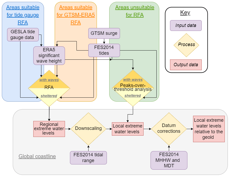
Figure 1 Schematic flow diagram detailing the data sources and processes involved in producing a global set of extreme water levels.

3.1 Data processing

The GESLA-3 dataset was filtered to sample appropriate input data by removing duplicates, gauges located in rivers (away from the coast), and gauges that failed quality control checks carried out by the authors of the dataset (such as suspected datum jumps). The surge component of GTSM-ERA5 at each record location is isolated from the water level time series using a tide-only simulation and superimposed onto a tidal time series created with FES2014, as the FES2014 tidal elevations performed better than those of GTSM in initial testing against in situ observations. The decision to use tides from FES2014 is further supported by the conclusion from Muis et al. (2020), in which the authors state the following. “It appears that biases increase in regions with a high tidal range, such as the North Sea, northern Australia, and the northwest of the United States and Canada, which could indicate that GTSM is outperformed by the FES2012 model that was used to develop the GTSR dataset.” Tidal time series were also computed at each of the coastline output locations for use in downscaling the regional outputs and for the bias and datum corrections of the local ESL.

Wave setup is the static increase in water level attributed to residual energy remaining after a wave breaks (Dean and Walton, 2010) and is therefore only observed in areas exposed to direct wave action. In this study, wave setup is approximated as 20 % H_s from the ERA5 reanalysis, following the recommendation from a review of numerous laboratory and field experiments (Dean and Walton, 2010, and previous related studies; Bates et al., 2021; Vousdoukas et al., 2016). Wave setup is assigned to the nearest record location using a nearest-neighbour approach. Wave setup is assumed to be absent in sheltered areas (e.g. bays and estuaries). To account for this, the global coastline is classified as either sheltered or exposed, and the final extreme water levels are drawn from an RFA that is processed with or without wave setup added in. To classify the coastline, each coastline point is evaluated to determine whether it is exposed from a minimum 22.5° angle over a fetch of 50 km. A total of 16 equal-angle transects are drawn, extending 50 km from each coastline point. If two or more adjacent transects do not intersect with land, the coastline point is considered exposed. Applying wave setup using this approach is an obvious simplification that has been used for ease of global application. In reality, wave setup is impacted by local bathymetry and coastal geometry, as well as by local wind and wave conditions. There are, however, other more complex methods for estimating wave setup that incorporate some aspects of bathymetry and coastal geometry, such as Stockdon et al. (2006).

To process the RFA with wave setup, daily maximum wave setup is added to the daily highest water levels. Where tide gauge records fall outside of the temporal range of the ERA5 data, a copula-based approach was used to fit a simple statistical model between daily peak water levels and daily max H_s, providing a prediction of the daily max H_s. The RFA is then executed as described below. Tide gauges are assumed to be located in sheltered regions, such as bays and estuaries; thus, tide gauge records are not impacted by wave setup.

3.2 Spatial discretisation of water level records into regions

Water level records are spatially clustered to form a potential pool from which regional exceedance levels can be characterised. To do this, the global coastline is divided into 1° by 1° grid cells, which are used as the regions to apply the outputs for each RFA. All record locations within a 400 km radius (as in Hall et al., 2016 and Sweet et al., 2022) of the grid cell centroid that have at least 10 consecutive years of good (>90 % completeness) data are identified (minimum of 3 water level records, maximum of 10; as in Sweet et al., 2022). This step is illustrated in Fig. 2a. Record locations which are geographically within range but are separated by a large expanse of land and thus likely forced by different storm patterns are removed from the record location selection. To achieve this, a line is drawn between the grid cell centroid and each record location. The land intersected by the line is divided, and the areas of land on either side of the line are summed. A ratio of the length of the line to the area of land segmented by the line is then calculated. A threshold of 100 was empirically evaluated using expert judgement based on a number of test cases, above which records are removed from the grid cell analysis. This approach ensures that, for example, record locations located on the east coast of Florida (e.g. Mayport) are not grouped with those on the west coast (e.g. Cedar Key) when characterising regional growth curves, despite the relatively short straight-line distance between them. Figure 2a exemplifies three tide gauges which have been excluded from possible selection despite lying within a 400 km radius of the grid cell centroid, as the area of land that separates them is large when compared to the distance. This spatial discretisation of regions results in a total of 836 tide gauge records (with a mean record length of 17 years) and 18 628 GTSM-ERA5 records for use in application of the RFA.

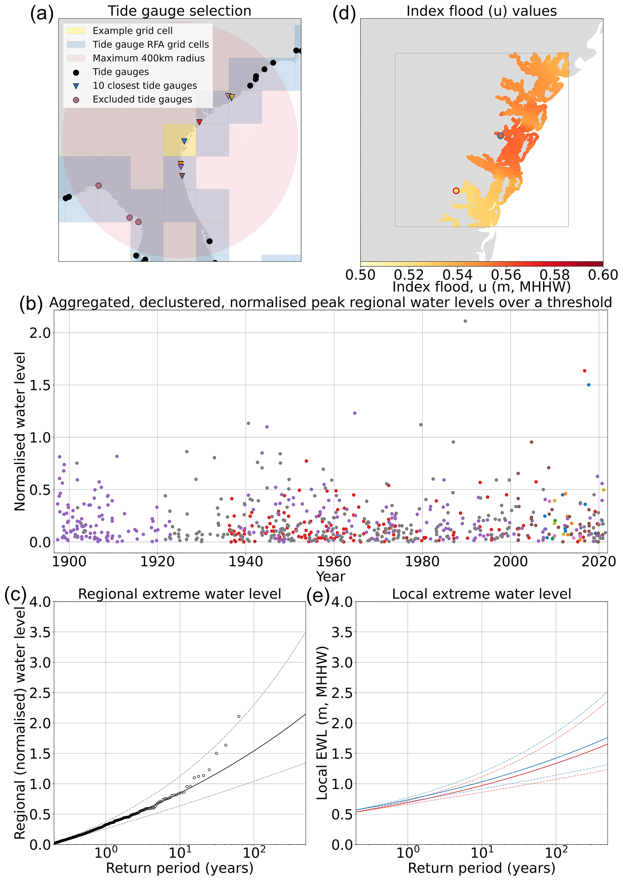
Figure 2 Selection of the steps in the RFA. (a) The 1° by 1° grid cells along the East Coast of the US, along with the locations of the tide gauges and the tide gauges selected for the RFA of the example grid cell. The tide gauges excluded from possible selection by the distance to land area ratio are also indicated. (b) The aggregated, declustered, normalised peak regional water levels over a threshold for each of the tide gauges used in the example grid cell. The colours indicate peak water levels from the individual tide gauges in the region. (c) Regional extreme water levels ascertained by fitting a generalised Pareto distribution to the data displayed in panel (b). (d) Index flood values of the example grid cell found by linearly interpolating the u value from the two closest tide gauges and scaling by tidal range. The locations of two coastline points used to produce local extreme water levels in panel (e) are also highlighted. (e) Local extreme water level at two shoreline points inside the example grid cell, each with different index flood values, as indicated in panel (d).

The RFA is preferentially applied to tide gauges in areas where the gauge density is sufficient (minimum of three gauges within a 400 km radius, as in Hall et al., 2016, and Sweet et al., 2022). Outside of these areas, the RFA is implemented using data from GTSM-ERA5. In some regions, the density of homogenous record locations from GTSM-ERA5 is also too low for the RFA to function, in which case the ESL exceedance probabilities are interpolated from a single-site peaks-over-threshold analysis of the nearest GTSM-ERA5 record location. The geographical locations of these areas are shown in Fig. 3. From the 5975 global coastal grid cells, ESLs at 851 are computed using tide gauge data, 4555 are calculated using RFA of GTSM-ERA5 data, and 569 are calculated using GTSM-ERA5 data from the nearest record location.

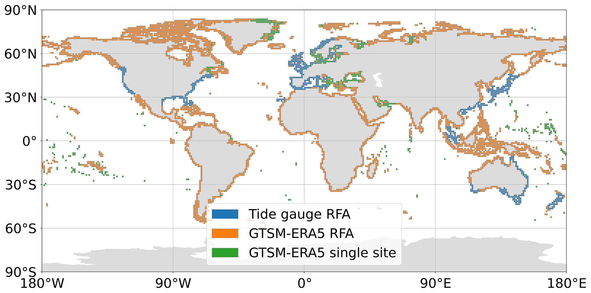
Figure 3 Map showing the global distribution of the areas in which the tide gauge RFA is used and in which the GTSM-ERA5 RFA is used, as well as the areas which represent interpolations of single-site analyses of GTSM-ERA5.

3.3 Application of the RFA

Tide gauge records are referenced to different vertical datums. Therefore, in order to ensure consistency, the mean taken over the most recent 19-year epoch is subtracted from the water level record, and the time series is linearly detrended to the centre year of the most recent available epoch (2002 to 2020), resulting in 2011. GTSM-ERA5 records are referenced to MSL over the period from 1986 to 2005, and so the time series are linearly detrended to reference the same tidal epoch as the tide gauge records centred on 2011. Within each cluster of gauge (or model) records, the water level time series are resampled to hourly resolution and converted to mean higher high water, defined as the mean daily highest water level over a 19-year epoch, to account for differences in tidal range between record locations. In the case of records with fewer than 19 years of data available, the maximum continuous epoch is used instead.

Daily highest water level is determined from the hourly time series of each measured or modelled record. The time series are then declustered using a 4 d storm window to ensure event independence. This window length was used by Sweet et al. (2020, 2022) and is of a similar length to the storms that cause surge events in the UK (Haigh et al., 2016). The index flood u, defined as the 98th percentile of the declustered daily highest water levels (Sweet et al., 2022), is used as the exceedance threshold at which to normalise the water level at each record location as follows:

$$\begin{array}{}\text{(1)}& \begin{array}{rl}& \text{Normalised\hspace{0.17em} water\hspace{0.17em} level}=(\text{observed\hspace{0.17em} exceedance\hspace{0.17em} }\\ & \text{water level}-u)/u.\end{array}\end{array}$$

The normalised datasets are then aggregated and further declustered to ensure that only one peak water level is retained for each regional event. This is shown in Fig. 2b for an example grid cell. Following Hosking and Wallis (1997), a statistical heterogeneity test (H) is undertaken to ensure the homogeneity of the region. If the H score is less than 2, then the region is considered sufficiently homogenous. If the H score is greater than 2, then the furthest water level record from the grid cell centroid is removed from the region, and the test is rerun. This process is repeated until the H score is less than 2. In a minority of cases, the heterogeneity test fails due to an anomalous record that lies within the closest three sampling locations to the grid cell centroid. In this instance, the test is rerun, except after the furthest record is removed, all the remaining records are sequentially removed and replaced until the H score is less than 2.

After the region has been confirmed to be homogenous, a generalised Pareto distribution is fitted to the aggregated, declustered, and normalised regional water levels using a penalised maximum likelihood method to estimate regional extreme water levels (REWLs). This is illustrated by an example in Fig. 2c. This is repeated for the aggregated regional water levels for each 1° by 1° grid cell. While theoretically correct, applying distribution fits to real-world data can sometimes give unrealistic results, particularly in terms of the estimation of the lower-frequency space. In these cases, growth curve optimisation is undertaken to ensure that the output local extreme water levels are plausible in real-world scenarios. To ensure consistency, an empirical threshold of 0.35 for the shape parameter is used to determine which curves will generate unrealistic extreme water levels. The empirical threshold of the shape parameter is determined based on expert judgement of plausible real-world maximum surge heights in the low-frequency events. To correct these curves, wherever this threshold is exceeded, we use the shape and scale parameters of the nearest grid cell which does have a shape parameter of less than 0.35. In total, 34 grid cells had their shape and scale parameters adjusted, most of which were concentrated in the Gulf of Mexico and Japan.

3.4 Downscaling to local extreme water levels

Local extreme water levels (LEWLs) are then estimated from the regional growth curves using the following relationship:

$$\begin{array}{}\text{(2)}& \text{LEWL}=\left(\text{REWL}\cdot u\right)+u.\end{array}$$

This is done for each coastal point along the coastline contained within the grid cell represented by the REWL records. The index u is estimated at the coastline points using an inverse distance weighting interpolation of the u values for the two closest record locations scaled by tidal range. This deviates from the methodology set out in Sweet et al. (2022), in which the authors recommend drawing u values from a linear regression of u against tidal range values from record locations across a region. We found this approach to lead to significant differences in LEWLs at record locations when compared to single-site analysis of water level records, and we have hence modified the methodology. Figure 2d exhibits an example of the index flood for every shoreline point in an example grid cell. Tidal ranges are calculated as the difference between the mean higher high water and the mean lower low water. Tidal harmonics from FES2014 are used to predict mean higher high water and mean lower low water at each coastline point. The index flood u is used to downscale the REWLs, which represent the ESL characteristics of the entire grid cell. The LEWLs are output in the format of return levels for a range of exceedance probabilities. Two example LEWL curves are shown in Fig. 2e, which have been computed using different index flood values, as indicated in Fig. 2d.

3.5 Bias and datum corrections

The last stage of the LEWL calculation involves characterisation and removal of bias in the high-frequency portion of the exceedance probability curves relative to a single-site analysis of water level records (within which we expect the high-frequency water levels to be accurately modelled). Other surge RFA studies also concluded that the approach generally yields higher estimated surge heights when compared to single-site analysis, because during the regionalisation process, an extreme event that occurred in one location is assumed to have the same probability of occurring at another location within the homogeneous region (Bardet et al., 2011; Sweet et al., 2022). Bias is quantified based on the divergence in the 1-in-1-year return period at each tide gauge or GTSM-ERA5 location and the corresponding LEWL predictions. This bias is used as a correction term and is removed from the LEWLs. As the density of the coastline points is much higher than the density of the tide gauges and model output locations, the correction term is interpolated across all coastal LEWL points based on the correlation between monthly values of the 99th percentile of tidal elevations – produced over a 3-year period centred on 2011 computed using FES2014 at the tide gauge or GTSM-ERA5 location – and the neighbouring coastline points. The mean bias correction across all gauges is 8 cm.

Datum corrections are applied to ensure that the LEWLs are correctly referenced to a vertical datum which can be used for hazard assessment applications, such as inundation modelling. Inundation models utilise digital elevation models, which typically reference a geoid as the vertical datum. The output water levels from the RFA are transformed from mean higher high water to mean sea level (m.s.l.) values by adding the approximation of mean higher high water (above m.s.l.) from the FES2014 simulations to each of the boundary condition points. The corrected MDT dataset from Mulet et al. (2021) is applied to convert water levels from MSL from the FES2014 model to the “MSL” of a commonly used geoid, EGM08.

3.6 Validation methods

In this section we define the range of validation techniques used to address objectives 3 and 4. To validate the RFA ESLs against tide gauge records from GESLA (objective 3), a comparison is performed against ESL exceedance probabilities calculated at the individual tide gauges used to inform the RFA. To quantify the degree to which the RFA approach improves the estimation of ESL exceedance probabilities compared to single-site analysis (objective 4), two assessments are made.

Firstly, the divergence between GTSM-ERA5 RFA ESLs and GTSM-ERA5 single-site ESLs for the entire global coastline is quantified. These are then contrasted against the differences between return levels from GTSM-ERA5 (Muis et al., 2020) and COAST-RP (Dullaart et al., 2021). The comparison can then identify regions in which the historical ESLs are poorly represented due to the limited record lengths.

Secondly, a leave-one-out cross-validation is undertaken using GTSM-ERA5 data. Leave-one-out cross-validation aims to address the common issues involved with validating statistical models. One common method to validate models is split-sample validation, in which the data are split into two groups, a training set and a validation set, which generally comprise 70 % and 30 % of the data, respectively. The model is then trained on the larger set and validated against the smaller set. The drawbacks of this method include a highly variable validation error due to the selection of the training and validation sets, as well as a validation error bias caused by training the model on only 70 % of the available data (James et al., 2013).

Instead of using a 70:30 split of the data, leave-one-out cross-validation uses a larger proportion of the data to train the model, while validating against a smaller subsample, but repeats this process multiple times to generate a robust validation. To do this, we identified 1000 grid cells which use 10 GTSM-ERA5 records for the RFA and contain three GTSM-ERA5 record locations inside the grid cell (and therefore the RFA can be used to directly estimate ESLs at the record locations). One of the GTSM-ERA5 records from inside the grid cell is removed from the RFA process, and the REWL is calculated using the nine remaining gauges. The LEWL is then predicted at the record location which has been left out using the index flood u at the record location. These LEWLs are then contrasted with a single-site analysis of the water level record that was removed from the RFA. The process is then repeated for the two other GTSM-ERA5 record locations which lie within the grid cell. This means that each of the 1000 models is tested three times – against 90 % of the available data – thus giving a more robust realisation of the model when trained on 100 % of the data.

4 Results

The Results section is divided into four subsections. Section 4.1 presents the results of the global application of the RFA, showing both the global view of two return periods and the return levels for selected sites around the world. Section 4.2 illustrates how the RFA methodology improves the characterisation of rare extreme events based on the example of Cyclone Yasi (objective 2). In Sect. 4.3 we validate the RFA against estimates of ESL from GESLA tide gauges (objective 3). Finally, in Sect. 4.4 we quantify the improvements made by using an RFA approach when compared to a single-site analysis of water levels (objective 4).

4.1 Global application of RFA

The final ESL exceedance probabilities (including wave setup) created at high resolution around the global coastline are displayed in Fig. 4 for the 1-in-10- and 1-in-100-year return periods. Both the 1-in-10-year (Fig. 4a) and 1-in-100-year (Fig. 4b) return periods show similar spatial patterns, with the 1-in-100-year return periods exhibiting greater increases, as expected, in areas prone to TC activity (e.g. the Gulf of Mexico, Australia, Japan, and China). ESLs are higher in regions with large tidal ranges such as the Bay of Fundy, the Patagonian Shelf, the Bristol Channel in the UK, the northern coast of France, and the northwest coast of Australia. The return levels for six selected tide gauge locations, three of which are characterised by a positive and three of which are characterised by a negative shape parameter from the generalised Pareto distribution, are shown in Fig. 4c and d, respectively, relative to mean higher high water. The locations of the six tide gauges are indicated in both Fig. 4a and b. Regions exhibiting positive shape parameters are typically prone to TC activity and associated surge and wave events. As a result, these regions experience more significant increases in return levels at higher return periods than regions with negative shape parameters. Regions characterised by negative shape parameters have different drivers of ESL events, for instance extratropical storm surges or tide-dominated ESLs (Sweet et al., 2020).

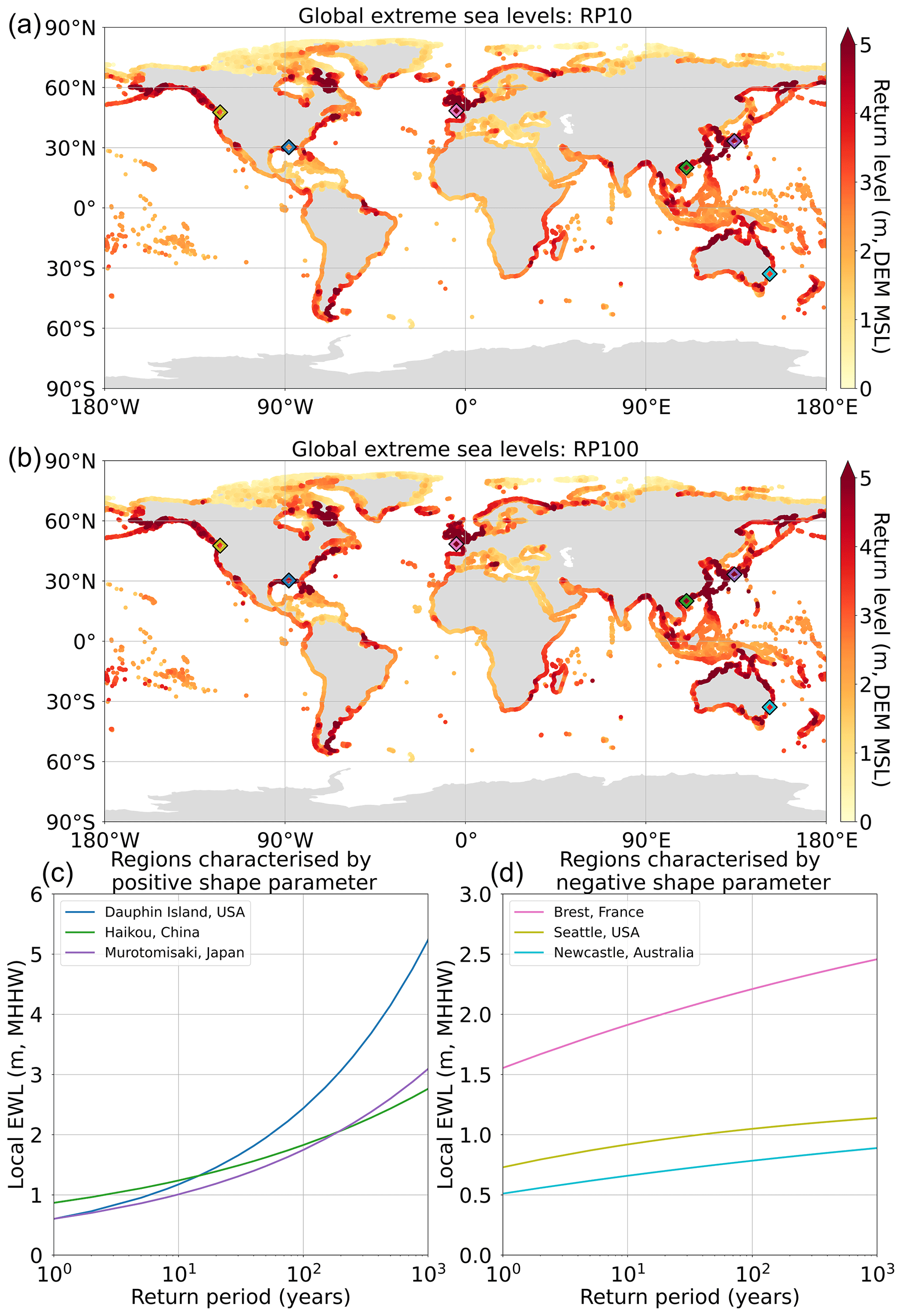
Figure 4 The final global output of RFA results at approximately 1 km resolution along the entire global coastline (excluding Antarctica) for RP10 (a) and RP100 (b). Return levels are referenced to DEM MSL and thus represent surge, waves, and tide. Return levels (relative to mean higher high water) for six tide gauges in regions characterised by either a positive or negative shape parameter from the generalised Pareto distribution are shown in panels (c) and (d), respectively. The locations of the six tide gauges are indicated by the diamonds plotted in panels (a) and (b).

4.2 Tropical Cyclone Yasi

Our second study objective is to illustrate how the RFA methodology previously described can draw upon a few rare events to provide a more realistic representation of low-frequency ESL exceedance probabilities across a region. This is done using the case study of Cyclone Yasi, which impacted the Australian coastline in 2011. Cyclone Yasi made landfall on the northeastern coast of Australia, in the Queensland region, between 14:00 and 15:00 UTC on 2 February 2011. It was the strongest cyclone to have impacted the region since 1918, with possible wind speeds of 285 km h⁻¹ and a minimum recorded pressure centre of 929 hPa (Australia Bureau of Meteorology, 2011). When it made landfall, Yasi was a category 4 storm on the Saffir–Simpson scale. The path and strength of the storm are shown in Fig. 5a.

The total water levels relative to mean higher high water are shown in Fig. 5b for all the tide gauges in the region. Compared to neighbouring tide gauges, Cardwell had the highest surge and the highest total water level by a considerable margin, receiving a surge of over 3 m above mean higher high water. Clump Point also showed a definitive but less substantial surge signal, whereas the other gauges showed much smaller surge effects or even no surge at all. The historical water level records of all the gauges in the regions are included in Fig. 5c. The tide gauges span different temporal ranges, and many have years which are incomplete. The longest record is at Townsville, which started in the late 1950s. Despite this long record, the largest documented event is Cyclone Yasi by over 1.5 m (at Cardwell).

Based on this historical record, no other surge event of this magnitude has impacted this section of coastline since records began. There are, however, records of other historical extreme events affecting the region that predate tide gauges. For example, Cyclone Mahina, which made landfall in Princess Charlotte Bay (approximately 100 km north of Cooktown) in 1899, reportedly had a surge height approaching 10 m (Needham et al., 2015). The idea that this stretch of coastline is at risk of TC-generated ESLs is further supported by STORM, a dataset of 10 000 years of synthetic hurricane tracks (Bloemendaal et al., 2020). IBTrACS shows just eight category 4 and 5 hurricanes impacting this 700 km stretch of coastline between 1980 and 2022 (shown in Fig. A2 in the Appendix; Knapp et al., 2010). In contrast, the STORM dataset has 333 events affecting the area, producing a more continuous spread of landfall locations along the coastline. In addition, large surges are sometimes not captured in this region due to the lack of gauges in rural areas (Needham et al., 2015).

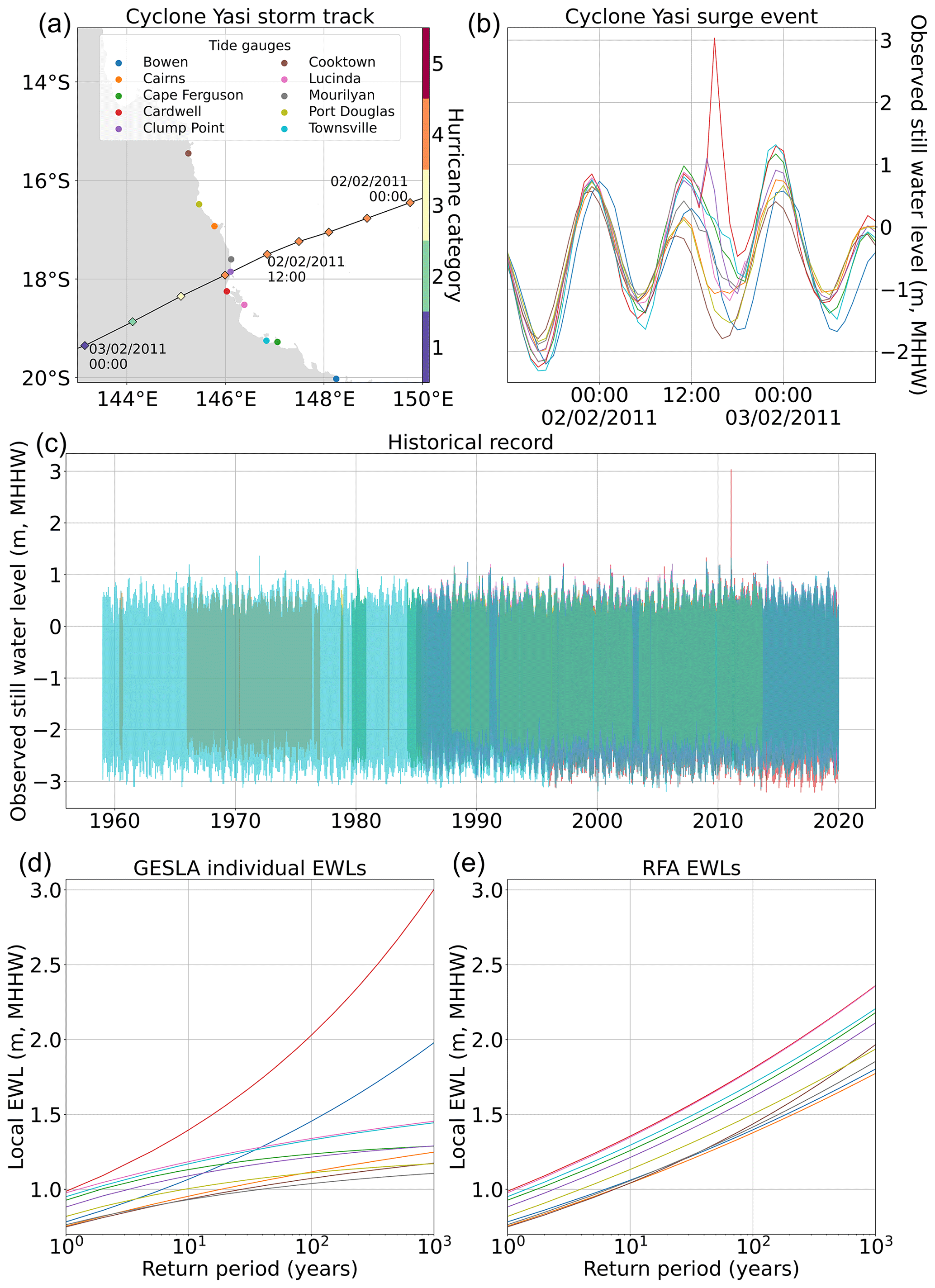
Figure 5 Tropical Cyclone Yasi. (a) Storm track of Cyclone Yasi, covering a 24 h period over the landfall event. The locations of the 10 closest tide gauges along the Queensland coast are also included. Times are in UTC. (b) Observed water level time series for the same 24 h period at each of the 10 tide gauges in the region. Times are in UTC. (c) Entire historical record of all 10 gauges in the region. (d) Return period curves of individual gauges fit with the generalised Pareto distribution. (e) Return period curves at the gauge locations from the RFA.

The return period curves for each of the 10 gauges in the region, calculated by fitting a generalised Pareto distribution to the peaks-over-threshold water levels at each individual tide gauge, are shown in Fig. 5d. As expected, Cardwell has the largest return levels and the steepest curve. All the other gauges, except Bowen, exhibit negative shape parameters, characterised by a decreasing gradient of the return period curves. In a region which is prone to TCs, this represents a dangerous underestimation of the risk from cyclone-induced surges. In some coastal ESL studies, ESLs are calculated at each gauge and then interpolated along the coastline, such as in the UK (Environment Agency, 2018). In this case, the latter approach would lead to a gross disparity from the actual risk of storm surges to coastal communities in the area.

In contrast, Fig. 5e shows the return period curves estimated from the RFA at the tide gauge locations. All of the curves now have positive shape parameters, characterised by increasing gradients of the curves. The curves of Cardwell and Bowen have been reduced somewhat, while all the other curves have been increased significantly. This demonstrates the regionalisation process by which the extreme event at Cardwell can be used to propagate the risk along the coastline to areas which do not have an extreme event on record or which have short, incomplete, or nonexistent tide gauge records. This reinforces the key strengths of RFA, namely (1) the ability to spatially account for rare extreme events, (2) the use of short and incomplete tide gauge records to produce robust parameter fits, and (3) the ability to downscale the results into regions which are not covered by tide gauges at all.

4.3 Comparisons with GESLA

The third objective is to validate ESLs calculated using our RFA against those calculated directly from the measured GESLA-3 global tide gauge database. Contrasting the RFA results with ESL exceedance probabilities calculated through a generalised Pareto distribution fit at individual tide gauges yields promising results. Figure 6a shows the spatial distribution of the difference at the 1-in-10-year return period for Europe, the United States, and the eastern Pacific. In areas impacted by TCs (e.g. the Gulf of Mexico, the northeastern coast of Australia, and Japan) we broadly see that the RFA has increasing return levels across most gauges. Increases in the 1-in-10-year return level are also observed in areas usually associated with extratropical storms (e.g. Europe), suggesting that gauges in these regions also suffer from undersampling of rare surge events. Extreme surge events can be undersampled for two reasons. Firstly, by their very nature, they are rare and might never have occurred at a specific location. Secondly, as a result of the scarcity of in situ tide gauges, surges can occur and remain unrecorded.

In all areas shown in Fig. 6a, some gauges show decreases in the return levels. These could be driven by either shape parameter limiting (to prevent unrealistically large water levels); an anomalously large number of events impacting the gauge; or a single anomalously large event impacting the gauge, which is then smoothed out through the regionalisation process, as was the case in Cardwell, Australia (Fig. 5e). Of the gauges shown in Fig. 6a, only five had limited shape parameters, and these were located in the Gulf of Mexico. The distribution of the differences at RP10 is shown in Fig. 6b with a positive skew, detailing the 5th and 95th percentiles as −8 and 27 cm, respectively. The spread of the data increases across the three selected return periods (1-in-2-, 1-in-10-, and 1-in-100-year return periods), as presented in Fig. 6c, as does the mean bias, which increased from 2 cm in the 1-in-2-year return level to 21 cm in the 1-in-100-year return level.

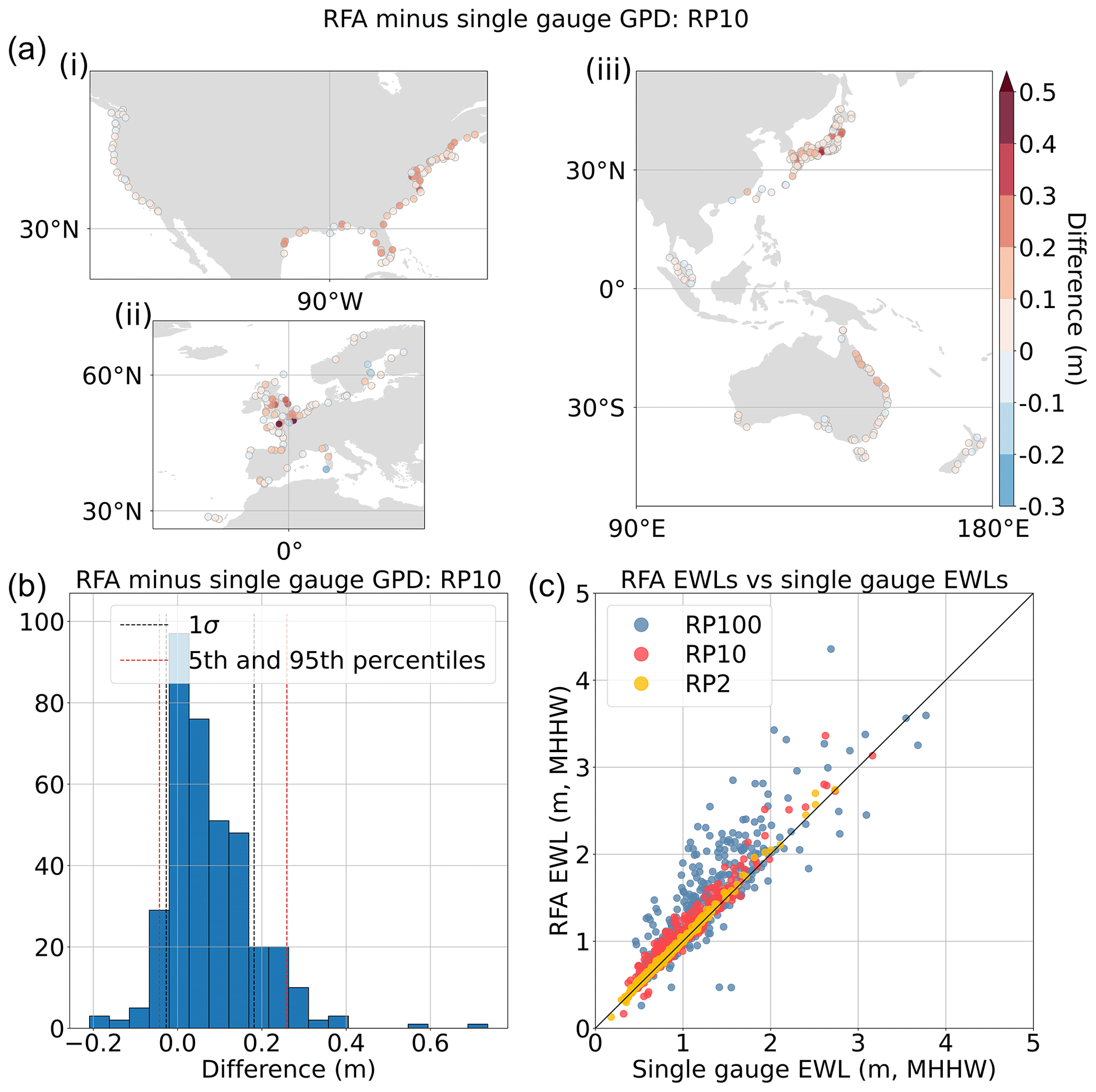
Figure 6 Comparison of RFA water levels against extreme water levels calculated at individual gauges from GESLA by fitting a generalised Pareto distribution to peaks-over-threshold water levels. (a) Spatial distributions of the differences at RP10 for (i) the contiguous US; (ii) Europe; and (iii) Japan, Malaysia, Australia, and New Zealand. (b) Histogram of the distribution of differences at RP10, including the locations of the 5th and 95th percentiles and 1 standard deviation from the mean. (c) Scatter plot of EWLs (RP2, RP10, and RP100) from the RFA and EWLs calculated using a single-site generalised Pareto distribution fit. The black line indicates a 1:1 perfect fit.

4.4 Quantifying the increases caused by RFA as compared to single-site analysis

The fourth objective is to quantify the increases in ESL exceedance probabilities in TC-prone areas caused by RFA as compared to single-site analysis. Figure 7a shows the deviation in the 1-in-100-year return period between the GTSM-ERA5 RFA carried out across the global coastline and a single-site peaks-over-threshold analysis of GTSM-ERA5 water level records. Only differences greater or less than 0.25 and −0.25 m, respectively, are plotted. There are evident increases in RFA ESLs in areas prone to TCs. The Gulf of Mexico, the East Coast of the US, southern China, and the northeast coast of Australia show the largest increases. Sporadic negative differences are also observed in Fig. 7a, which are driven by a smoothing of ESL exceedance probabilities at locations which have experienced anomalously high ESLs compared to the local region. From this we see that the RFA is capable of incorporating the influence of TCs that were not present in the historical record but statistically could occur, as indicated by the regional characteristic.

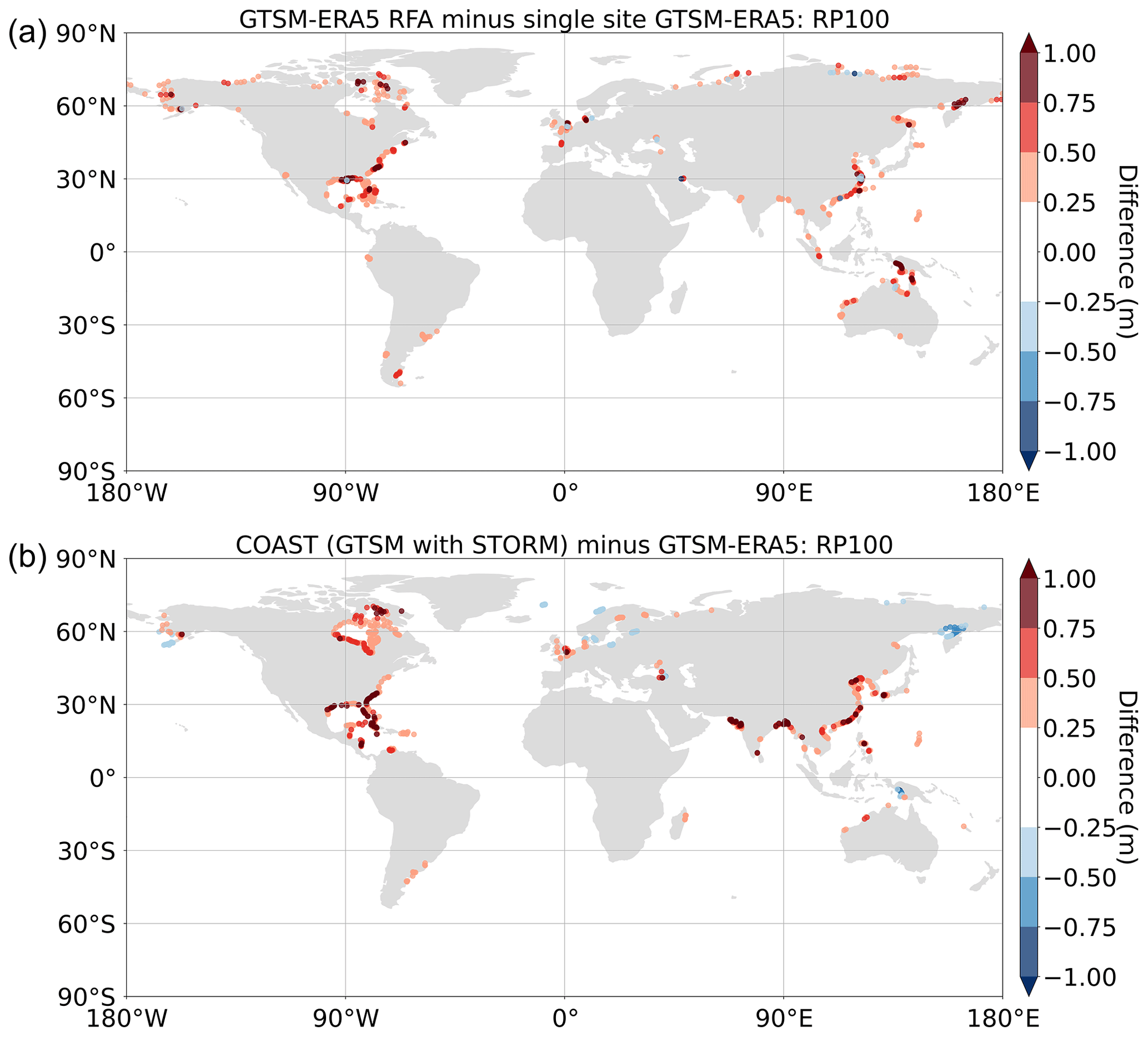
Figure 7 Spatial distribution of (a) the differences between the GTSM-ERA5 RFA 1-in-100-year return period (RP100) and the RP100 of single-site GTSM-ERA5 data fitting with a generalised Pareto distribution to the peaks-over-threshold water levels and (b) the differences in RP100 published by the COAST-RP (GTSM forced with STORM) paper (Dullaart et al., 2021) and RP100 published by the original GTSM paper (Muis et al., 2020). Only differences greater or less than 0.25 and −0.25 m, respectively, are plotted.

These findings are supported by the results presented in Fig. 7b, which shows the differences between COAST-RP and GTSM-ERA5. COAST-RP is GTSM forced with STORM (10 000 years of synthetic TCs) in areas prone to TC activity rather than with ERA5 (Dullaart et al., 2021). The areas of positive difference highlight locations where COAST-RP is greater than GTSM-ERA5 and thus give an indication of the areas in which the synthetic hurricanes make landfall. These patterns are broadly similar to those of the RFA shown in Fig. 7a. However, there are two areas which stand out for being poorly characterised by the RFA: the Bay of Bengal and the western Gujarat region of India. Large differences are also observed in Hudson Bay, Canada; however, we suspect that these discrepancies are the result of differences in the approach to modelling extratropical regions, as TCs do not make landfall here.

Figure 8 shows the results of the leave-one-out cross-validation of the global coastal LEWLs. In general, the RFA tends to increase return levels due to the regionalisation process. These findings match those of Sweet et al. (2022, 2020), the work upon which our approach is based. This is evident throughout the world, with the majority of gauges exhibiting increases of less than 5 cm at the 1-in-10-year return period (Fig. 8a). The central 90th percentile band of the data for the 1-in-10-year return period ranges from −3 to 18 cm, as shown in Fig. 8b. However, the spread of the data is more pronounced at the higher return periods, as shown in Fig. 8c. Some regions of the world have greater increases, of the order of 30 to 40 cm, for the 1-in-10-year return period. These gauges are mostly concentrated in TC basins, namely the Caribbean, the Gulf of Mexico, Japan, China, and the Philippines, as well as on the east and west coasts of Australia. This demonstrates the process by which the RFA better represents extreme rare events that are typically undersampled in the historical record. By drawing on all the events captured by gauges across the region, the RFA reveals that a greater risk of extreme events manifests upon considering their potential occurrence in areas that, by chance, have not been previously impacted according to historical records. Similarly, oversampling is clearly evident at the 1-in-100-year return period, for which nearly one-third of locations show decreases in ESL exceedance probabilities compared to the single-site analysis. The magnitude of these decreases tends to be much smaller than the increases seen.

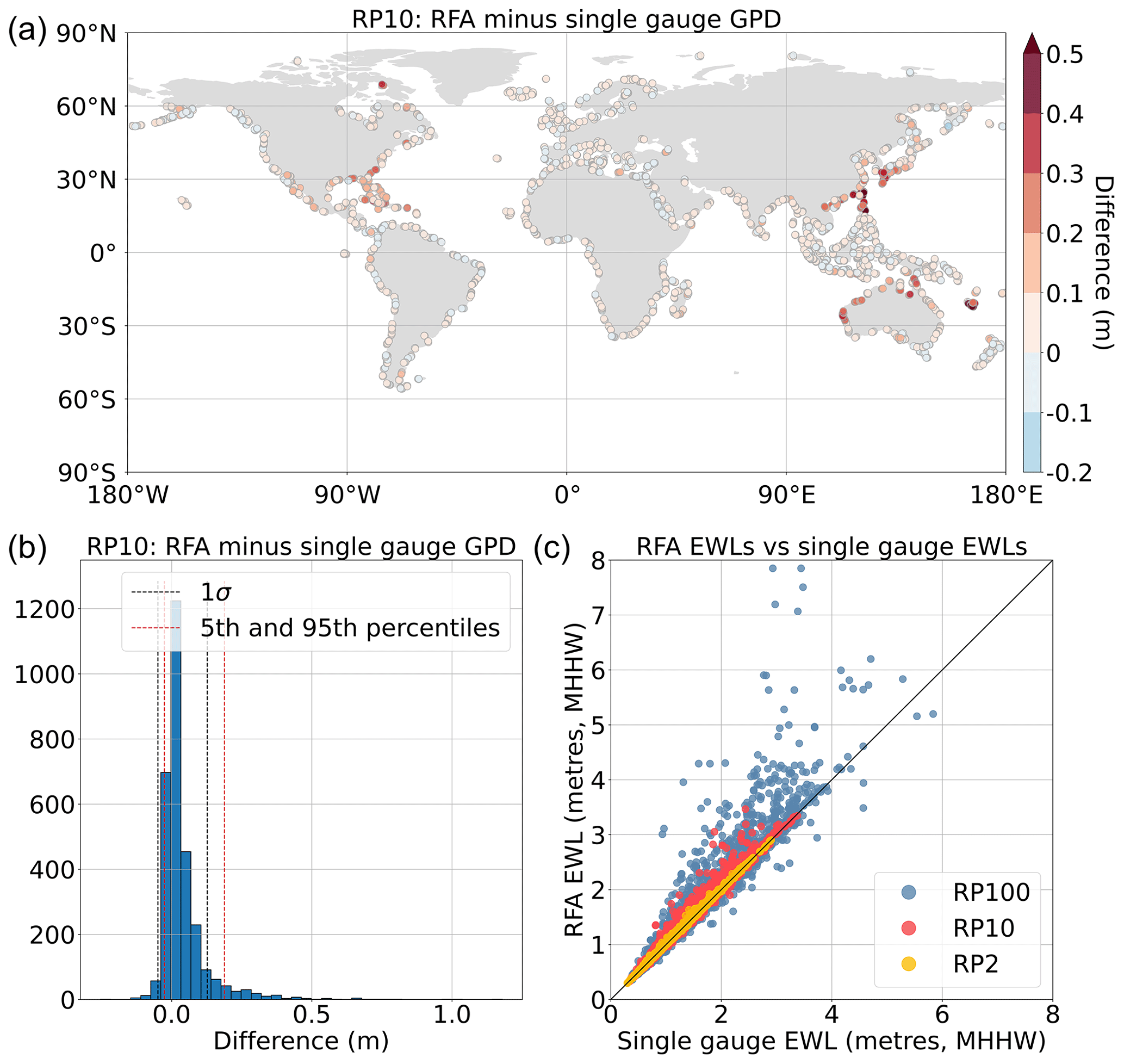
Figure 8 Results of the leave-one-out cross-validation of the RFA on GTSM-ERA5 gauges. (a) Spatial distribution of differences between the leave-one-out cross-validation RFA RP10 (1-in-10-year return period) and the single-site generalised Pareto distribution RP10. (b) Histogram of the distribution of the differences in RP10, including the locations of the 5th and 95th percentiles and 1 standard deviation from the mean. (c) Scatter plot of EWLs (RP2, RP10, and RP100) predicted using the leave-one-out cross-validation RFA and the EWLs calculated using a single-site generalised Pareto distribution fit. The black line indicates a 1:1 perfect fit.

5 Discussion

The ESL exceedance probability dataset presented in this paper is, to our knowledge, the first global dataset to be derived using an RFA approach employing a synthesis of observed and modelled hindcast data. The resulting data are output at high resolution (∼1 km) along the entire global coastline (excluding Antarctica); they include wave setup data and better capture the coastal flood risk from TCs. This approach is notable for being computationally inexpensive compared to more traditional approaches for deriving ESL exceedance probabilities via hydrodynamic modelling.

As previously discussed in the Introduction section, relying solely on observational records to estimate ESL exceedance probabilities can significantly bias results. To fit robust parameter estimates and obtain confident exceedance probabilities sufficient for informing flood risk managers, long-term and consistent high-quality observational records are needed (Coles, 2001). While some tide gauge and wave records span numerous decades, many records only cover a handful of recent decades (e.g. 10 to 30 years) or have significant gaps in their historical records. This means that high-quality data are often excluded from analyses as their records are too short to produce robust parameter estimates. Furthermore, gauges are relatively sparse, especially in less populated areas and developing nations. While surges and waves typically impact large regions, peak water levels are usually only observed over smaller areas (i.e. a single bay, estuary, or beach). As a result, measured records can easily miss the maximum of an extreme event and thus mischaracterise the extreme water levels of the event. As such, rare extreme events that characterise the upmost tails of the distributions of ESLs, such as TCs, are repeatedly undersampled in the historical record in terms of both frequency and magnitude.

Using an RFA approach, we demonstrate how we have improved these issues. The RFA can be viewed as a space-for-time approach, where long historical records (which give robust parameter estimates) are substituted for a collection of shorter records that cover a larger area. The volume of data (and subsequent extreme events) is retained, but the individual records can be much shorter. In this study, records as short as 10 years have been utilised. Furthermore, the regionalisation process works to overcome the issues with gauge density by disseminating the hazard presented by rare extreme events, as shown using the example of Cyclone Yasi. Of the 10 gauges in the region, the only record to have captured an historical extreme surge event of the magnitude observed during Cyclone Yasi was Cardwell, despite this section of coastline being at a known risk of TC activity. A single-site analysis of tide gauge data in this region would likely underpredict the real risk of ESLs generated by TCs in areas which have not experienced a direct impact according to the observational record. On the other hand, the damping of the return levels in the RFA output at Cardwell and Bowen could result in an underprediction of the risk from surges in these locations.

Global hydrodynamic models that simulate tide and surge (e.g. GTSM) or waves have been developed to substitute observational records, especially in regions not covered by tide gauges. These models have been demonstrated to represent historical extreme events to a high degree of accuracy when forced using historical observational data pertaining to the event (Yang et al., 2020). However, using these models for characterisation of exceedance probabilities is limited by the availability of long-term high-quality global reanalysis data that capture the full extent of meteorological extremes that drive large surge events. The RFA aims to address this by using a space-for-time approach; however, it is still limited by the bounds of the GTSM-ERA5 data. As demonstrated in Fig. 7, the distribution of increases to local return levels resulting from RFA broadly follows the same patterns globally as the differences between COAST-RP and GTSM-ERA5. As the TC hazard is typically underrepresented due to short records, it can be inferred that the increases observed across these regions are an improvement over single-site analysis.

While RFA is capable of identifying areas at increased risk from TC activity, it is still constrained by the available training data. This is demonstrated in Fig. 7. Two distinct areas lack increased water levels in the RFA difference plot (Fig. 7a): the Bay of Bengal and the northwestern coasts of India and Pakistan. ERA5, the source of the forcing data used for GTSM-ERA5, has been found to consistently underestimate TC intensity in terms of both minimum sea level pressure and maximum wind speed (Dulac et al., 2023). Consequently, the intensity of extreme events in GTSM-ERA5 in these regions could underrepresent the potential hazard from TC activity. If the maxima of extremes are not captured in the reanalysis data, then the full magnitude of the surge cannot be simulated by GTSM-ERA5. As such, the RFA will have smaller or fewer extremes from which to draw data when characterising rare extreme events, thus leading to a persistent underestimation of the return levels.

Coastal flood hazard mapping is usually carried out using inundation models that simulate the propagation of water over the coastal floodplain. To accurately capture the footprint of the surge on the land, inundation models require high-resolution boundary conditions at regular intervals along the coastline. The density of boundary condition points must be sufficient to capture local variability in ESLs along a coastline, which can be caused by bathymetrical and topographical features such as narrow channels, enclosed bays, barrier islands, and estuaries. The spatial resolution of tide gauges, even in the areas of highest gauge density, is insufficient for direct use in inundation modelling and therefore requires some form of interpolation and/or extrapolation. Similarly, while GTSM-ERA5 is run at a reasonably high coastal resolution, publicly available data are only output at approximately 50 km resolution outside of Europe and therefore do not meet the standards necessary for coastal floodplain inundation modelling. Using RFA to downscale the regional extreme water levels allows for the possibility of implementing tide gauge data and the outputs from GTSM-ERA5 as boundary conditions for subsequent inundation models. In addition, the downscaling process involves scaling the water levels by tidal range and thus enables dynamic characteristics of the surge, such as amplification at the head of estuaries, to be reproduced in the inundation models. This downscaling process is, however, limited by the resolution of the tide model used to obtain the tidal range values. In the case of the current study, FES2014 is output at $\mathrm{1}/\mathrm{16}$th of a degree (approximately 7 km at the Equator).

Ultimately, the future of delineating the flood hazard from TCs lies in multi-ensemble models using hundreds of thousands of years' worth of synthetically generated storms forcing high-resolution tide–surge–wave models. However, the computational cost of running such simulations is enormous when compared to the cost of running an RFA on a relatively short hindcast record. In the same way, dynamically modelled waves are usually excluded from global simulations that consider exceedance probabilities due to the computational expense. At the same time, failing to consider the joint dependence of surge and waves can lead to an underestimation of ESL exceedance levels by up to a factor of 2 along 30 % of the global coastline (Marcos et al., 2019). This reinforces the significance of the RFA methodology for characterising global coastal flood risk.

Validating the RFA is nuanced, as assessing metrics compared with the observed record (a) comprises a validation of the RFA against the data used to build the RFA in the first place and (b) does not recognise the inadequacies of the tide gauge records that the RFA is attempting to mitigate. Leave-one-out cross-validation highlights the strengths of the RFA without succumbing to the shortfalls inherent in the observational record. The increased LEWLs in the regions prone to TC activity once again demonstrate the ability of RFA to spatially disperse the hazard of low-probability extreme events across a region. It is worth noting that the leave-one-out cross-validation is the best possible representation of the RFA, as only grid cells that use data from 10 record locations are used, and each model is thus trained on the maximum amount of data possible. In some areas, the number of records used can be as low as three, and so the ability of the RFA to reproduce water levels in these regions could be compromised.

Applying the RFA as done in this study does have its limitations. Firstly, changing our definition of a homogeneous region would likely have a great impact on our results. In future iterations of this study, we recommend carrying out a sensitivity analysis to understand how using different maximum radii to select water level records impacts estimated extreme water levels within the region. Secondly, delineating the global coastline into 1° by 1° tiles and evaluating a different RFA for each tile results in some complex areas of coastline being summarised by a single regional growth function. Examples of this are seen in Japan, where exposed coastlines of the north coast are contained in the same tile as a sheltered bay that is open to the south coast. A solution to this would be to classify coastlines based on descriptors, as carried out by Sweet et al. (2020). These descriptors could include characteristics such as the dominant forcing type, geographic location, and/or local coastal dynamics. The method used to incorporate wave setup is another constraint, as it has been greatly simplified for ease of global application. Improving upon this should also be a focus of future studies. Lastly, another limitation of the approach used in this study is the static shape parameter limiter. It is probable that the maximum shape parameter varies by location around the world and that by implementing a fixed threshold globally, we are perhaps limiting some of the most extreme events in some regions. Improving this section of the methodology is a high priority for future updates.

The outputs from the RFA should be supplemented with local knowledge wherever possible, and the uncertainties in the results should be considered before the data are used. While RFA is a powerful tool for estimating return levels in ungauged locations or in locations where the historical records are short or incomplete, there are risks associated with both over- and underprediction of surge heights. Underprediction can lead to complacency among coastal managers and the potentially dangerous assumption that communities are safe from surge risk. Conversely, overprediction can result in unnecessary costs for risk mitigation measures and potential economic loss driven by a lack of investment in a region deemed to be at risk. Disseminating the risk of TC-generated surges over a region could lead to overprediction in some locations; therefore, conducting sensitivity analyses to understand the robustness of findings is recommended, especially in the context of coastal management and safety assessments. The RFA has been developed in this study as a method for regional- to continental- to global-scale risk analyses from globally available data and not for local studies. The results give a first-order approximation of extreme water levels in ungauged locations. It is not expected that they would be used for design of local flood defences, for example.

Going forward, the RFA framework developed in this study can easily be updated upon availability of new data. Possible next steps could also include using GTSM simulations of future climate scenarios and applying measured wave data. To this end, a global wave dataset similar to GESLA would be instrumental in collating wave data from the numerous global buoys. Future updates could also include an assessment of using different extreme-value distributions, perhaps following the mixed-climate approach of O'Grady et al. (2022).

In the near future, we plan to use the global exceedance probabilities derived in this paper as boundary conditions for inundation modelling of the coastal floodplain of the entire globe using the 2D hydraulic model LISFLOOD-FP (Bates et al., 2010). This presents an exciting opportunity to provide an invaluable resource that will help to better quantify global coastal flood risk.

6 Conclusions

In this paper we have demonstrated using an RFA approach utilising both measured and modelled hindcast records to estimate ESL exceedance probabilities, including wave setup, at high resolution (∼1 km) along the entire global coastline (with the exception of Antarctica). Our methodology is computationally inexpensive and is more effective in accurately estimating the low-frequency exceedance probabilities that are associated with rare extreme events compared to approaches that consider data from single sites. We have demonstrated, using the example of Cyclone Yasi (2011) which impacted the Australia coast, the ability of RFA to better characterise ESLs in regions prone to TC activity. Furthermore, on the global scale we have exemplified how the RFA, when trained on relatively short-term reanalysis data, can reproduce patterns of increased water levels similar to those present in dynamic simulations of 10 000 years of synthetic hurricane tracks. The RFA methodology shown provides a promising avenue for improving our understanding of coastal flooding and enhancing our ability to prepare for and mitigate its devastating impacts. In the future, we plan to use the exceedance probabilities from this study as boundary conditions for an inundation model covering the global coastal floodplain.

Appendix A

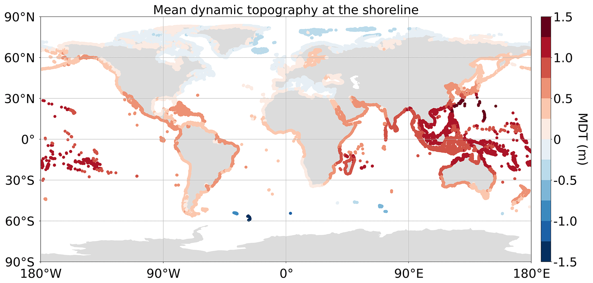
Figure A1 HYBRID-CNES-CLS18-CMEMS2020 MDT dataset from Mulet et al. (2021), extracted at the shoreline for use in correcting the output from the RFA for future uses such as inundation modelling.

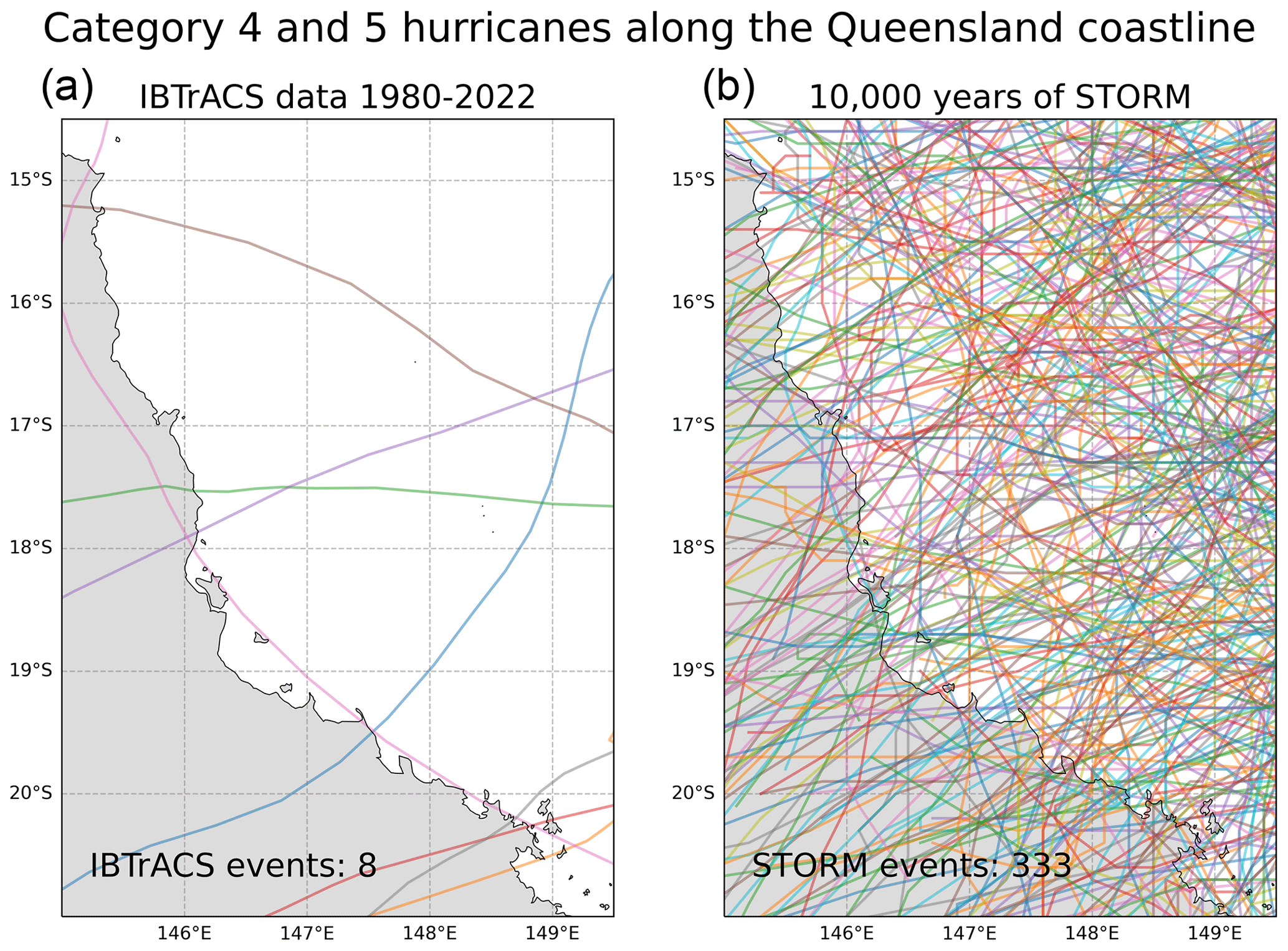
Figure A2 (a) Category 4 and 5 IBTrACS hurricanes impacting the Queensland coastline between 1980 and 2022 (Knapp et al., 2010) and (b) equivalent STORM events impacting the same the stretch of coastline (Bloemendaal et al., 2020).

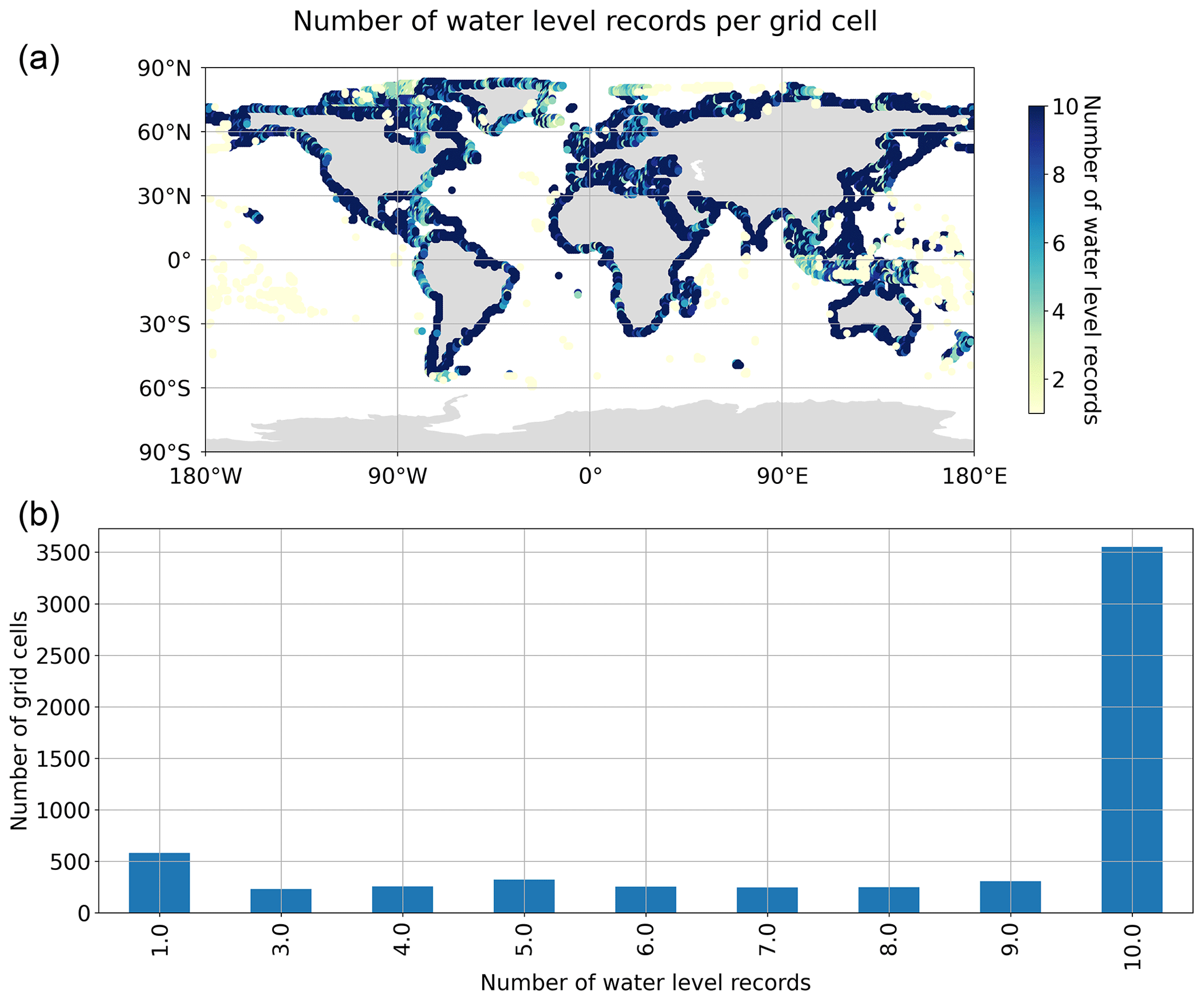
Figure A3 Number of water level records used per grid cell (a) as a scatter plot showing the distribution globally and (b) as a bar plot showing the number of water level records vs. the number of grid cells.