the Creative Commons Attribution 4.0 License.
the Creative Commons Attribution 4.0 License.
 | 16 Jul 2024
Comparing components for seismic risk modelling using data from the 2019 Le Teil (France) earthquake
Konstantinos Trevlopoulos
Pierre Gehl
Caterina Negulescu
Helen Crowley
Laurentiu Danciu
Probabilistic seismic hazard and risk models are essential to improving our awareness of seismic risk, to its management, and to increasing our resilience against earthquake disasters. These models consist of a series of components, which may be evaluated and validated individually, although evaluating and validating these types of models as a whole is challenging due to the lack of recognized procedures. Estimations made with other models, as well as observations of damage from past earthquakes, lend themselves to evaluating the components used to estimate the severity of damage to buildings. Here, we are using a dataset based on emergency post-seismic assessments made after the Le Teil 2019 earthquake, third-party estimations of macroseismic intensity for this seismic event, shake maps, and scenario damage calculations to compare estimations under different modelling assumptions. First we select a rupture model using estimations of ground motion intensity measures and macroseismic intensity. Subsequently, we use scenario damage calculations based on different exposure models, including the aggregated exposure model in the 2020 European Seismic Risk Model (ESRM20), as well as different site models. Moreover, a building-by-building exposure model is used in scenario calculations, which individually models the buildings in the dataset. Lastly, we compare the results of a semi-empirical approach to the estimations made with the scenario calculations. The post-seismic assessments are converted to EMS-98 (Grünthal, 1998) damage grades and then used to estimate the damage for the entirety of the building stock in Le Teil. In general, the scenario calculations estimate lower probabilities for damage grades 3–4 than the estimations made using the emergency post-seismic assessments. An exposure and fragility model assembled herein leads to probabilities for damage grades 3–5 with small differences from the probabilities based on the ESRM20 exposure and fragility model, while the semi-empirical approach leads to lower probabilities. The comparisons in this paper also help us learn lessons on how to improve future testing. An improvement would be the use of damage observations collected directly on the EMS-98 scale or on the damage scale in ESRM20. Advances in testing may also be made by employing methods that inform us about the damage at the scale of a city, such as remote sensing or data-driven learning methods fed by a large number of low-cost seismological instruments spread over the building stock.
- Article
(2664 KB) - Full-text XML
- BibTeX
- EndNote


Earthquakes are among the disasters with the most severe consequences, which include loss of human life, disruption of critical infrastructures, and insured and uninsured direct economic losses, as well as socio-technical impacts in multi-risk safety contexts. Assessments based on probabilistic seismic hazard analysis (PSHA) and probabilistic seismic risk analysis (PSRA) are key elements of efforts to improve awareness of seismic risk, earthquake response, and resilience to earthquakes. As far as seismic hazard and risk in Europe is concerned, the 2020 European Seismic Hazard Model (ESHM) and 2020 European Seismic Risk Model (ESRM20; Crowley et al., 2021a; Danciu et al., 2021) are state-of-the-art models, which were created by the European Facilities for Earthquake Hazard and Risk consortium. The predictive accuracy of the multi-component ESHM20 and ESRM20 models, like that of all seismic hazard and risk models and that of all statistical and probabilistic models, needs to be evaluated, despite the fact that the individual components comprising them have already undergone evaluation.
In the nuclear industry, testing and evaluation of PSHA models and their components have been formalized in the form of Senior Seismic Hazard Analysis Committee (SSHAC) hazard studies (Ake et al., 2018). SSHAC projects aim to produce technically defensible distributions and probabilities of exceedance of ground motion intensity measures. Bommer et al. (2013) tested ground motion models and their logic tree by comparing their implementations by three independent teams of modellers. As far as the evaluation of PSHA logic trees is concerned, Marzocchi et al. (2015) argue that the hazard should be considered to be an ensemble of models, which do not need to be mutually exclusive and collectively exhaustive. Rood et al. (2020) used observations of geomechanical failures, i.e. rock toppling, to estimate upper limits of ground motion intensity measures and constrain hazard estimations for long return periods. Their procedure always leads to a reduction in the seismic hazard estimation, which depends on the model for the seismic fragility, i.e. the model estimating the probability of geomechanical failure conditioned on a ground motion intensity measure. Moreover, they proposed a procedure for dropping branches of the PSHA logic tree and reweighting the remaining. Gerstenberger et al. (2020) note that tests of national or regional hazard models are only meaningful at the level of the site and that resorting to conversions of macroseismic intensity to ground motion intensity when ground motion records are lacking may introduce errors. Nevertheless, Mak and Schorlemmer (2016) did use such a conversion after testing the conversion equation itself.
In this study, to evaluate components used in seismic risk modelling, we use observations of damage to buildings in the municipality of Le Teil, France, caused by the 2019 Le Teil earthquake. Section 2 focuses on the interpretation of post-earthquake assessment damage data acquired for a small sample of buildings in terms of a three-level scale (i.e. a scale using green, yellow, and red colour tags) applied to EMS-98 damage grades. In Sect. 3, we detail the various assumptions and modelling choices with respect to the components of the damage calculation chain that we investigate, namely the various source rupture models, building exposure models, and ground motion models (GMMs) along with the site amplification models.
Subsequently, in Sect. 4, we make a series of comparisons based on ground motion intensity, macroseismic intensity, and damage distribution. For the comparison based on ground motion intensity, we generate samples for a set of ground motion intensity measures (IMs) estimated by scenario computations or shake-map methods (Wald et al., 2022) for rupture parameters reported by different sources. Shake maps are employed due to their capability to take into account any available ground motion records or macroseismic observations in the interpolation of the estimated shaking. Subsequently, we convert the IMs to macroseismic intensities using different ground motion intensity conversion equations (GMICEs). A third-party macroseismic intensity estimation for the municipality of Le Teil, provided by detailed on-site investigations (Schlupp et al., 2022), is then used to select the rupture parameters that lead to the most compatible macroseismic intensities and which are used in the scenario damage calculations.
Finally, in Sect. 5, we perform three types of comparisons based on probabilities of EMS-98 damage grades: (i) comparisons based on a building-by-building model, (ii) comparisons based on aggregated exposure models, and (iii) a comparison using different risk analysis tools (Armagedom – Sedan et al., 2013; the OpenQuake Engine – Pagani et al., 2014; Silva et al., 2014). In the first two types, we use alternative VS30 (the time-averaged shear-wave velocity up to a depth of 30 m) models to compare their effects on the estimated damage. The VS30 models used are the ESRM20 topography-based model and a geology-based model specific to France (Monfort and Roullé, 2016). In addition to VS30, the slope and the geology are used to account for ground motion amplification due to local site effects. In the comparisons using aggregated exposure models, the exposure models used are the ESRM20 exposure model, an aggregated exposure model based on French statistical data, and a building-by-building exposure model based on field damage observations. The probabilities of the damage estimated based on the calculations are compared to the corresponding probabilities based on damage observations and expert judgement. The steps leading up to these comparisons are summarized in Fig. 1.
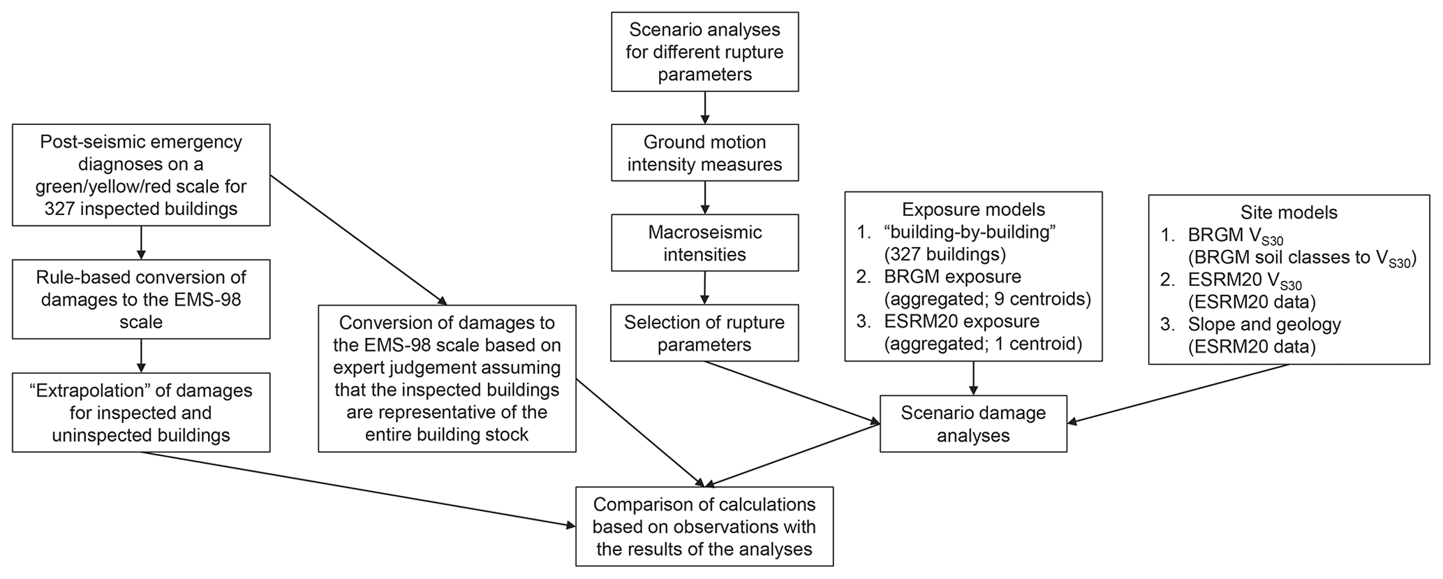
Figure 1Overview of the steps leading up to the comparison of the different estimations of the damage.
2.1 Seismic hazard and information for 2019 Le Teil earthquake
The municipality of Le Teil is located in southeastern mainland France, a region that corresponds to low- and moderate-risk categories according to the French seismic zonation. For Le Teil in particular, ESHM20 estimates a mean peak ground acceleration (PGA) of 0.04 g with a 0.21 % probability of exceedance in 1 year (475-year mean return period) under rock site conditions ( 800 m s−1).
The Le Teil earthquake took place on 11 November 2019, and its epicentre is located at 44.518° N, 4.671° E (Ritz et al., 2020), with a focal depth of 1 km and a moment magnitude Mw of 4.9 (Ritz et al., 2020), in close proximity to the municipality of Le Teil and the town of Montélimar in the lower Rhône valley in France. A private power plant accelerometer, located 15 km north-northeast of the epicentre and the closest seismic station to the earthquake, recorded PGA of 0.045 g (Schlupp et al., 2022). Three stations of the French seismological and geodetic network (Résif/Epos-France) at 24–44 km from the epicentre recorded PGAs in the range of 0.004–0.007 g. These four stations are at such a distance from the epicentre and the municipality of Le Teil that they cannot accurately constrain the predicted IMs. Causse et al. (2021) used numerical modelling, including physics-based rupture modelling and modelling of near-fault wave propagation, and estimated near-fault PGAs with a 68 % confidence interval of 0.3–1.9 g in the fault projection on the ground surface. They argued that their estimations are compatible with displacements of rigid block objects such as rocks and ledger stones. Moreover, they suggested that existing ground motion models may not be useful in the case of earthquakes such as this one, with a rarely observed shallow hypocentral depth, and with rupture parameters such as stress drop that are usually associated with earthquakes not only at larger depths, but also of larger magnitudes. However, it should be noted that some branches in the ESHM20 ground motion models logic tree should be able to account for the possibility of having extreme stress parameter values by treating uncertainty in the stress drop as a source of epistemic uncertainty (Kotha et al., 2020; Weatherill et al., 2020). As far as the attenuation of the intensity of the PGA is concerned, the recorded value at 15 km was 0.04 g, which indicates a high attenuation probably due to the very shallow rupture: the Le Teil earthquake is a specific event that generated very high, large intensities right next to the epicentre; however the ground motion was attenuated very quickly.
Schlupp et al. (2022) reported an EMS-98 macroseismic intensity of 7–8 for the municipality of Le Teil. This conclusion was the product of expert judgement considering the EMS-98 definitions of the intensity degrees and damage grades, the field observations from the Macroseismic Response Group, and the EMS-98 vulnerability classes of the buildings based on land registration data. Based on this procedure, Schlupp et al. (2022) determined 765 macroseismic intensities covering the area affected by the earthquake. The isoseismal line of the map by Schlupp et al. (2022) for intensity 7 includes the built area of Le Teil: given the limited spatial extent of this area, there is practically no spatial variation in the macroseismic intensity within this isoseismal line, and the maximum is at Le Teil (7.5).
2.2 Post-seismic emergency assessment dataset
We produced the dataset used here by processing post-seismic emergency inspection forms and by completing and editing an existing dataset (Perez, 2020) for 501 inspected buildings. The inspection forms were filled in by the French Association for Earthquake Engineering (AFPS) during on-site inspections (Taillefer et al., 2021), which took place from 3 to 5 February 2020. Out of the 501 buildings, the dataset produced contains 327 entries with information about the coordinates of each inspected building, the number of storeys, the date of construction, and the description of damage for the entirety of each inspected building as well as for its structural and non-structural elements. The colour tags assigned by the post-seismic emergency assessments are on a three-level scale, i.e. green–yellow–red, which we converted to EMS-98 damage grades. The 174 entries that were not included in the produced dataset were left out due to the fact that, although they included the colour tag for the building, they lacked information with respect to the damage to the structural elements and the non-structural components or with respect to the construction material, the year of construction, or the number of storeys. The distribution of the green–yellow–red tags across these entries (Table A5) has small differences from the distribution of the 327 entries (Table 2), which leads us to believe that their removal from the dataset does not introduce any significant bias.
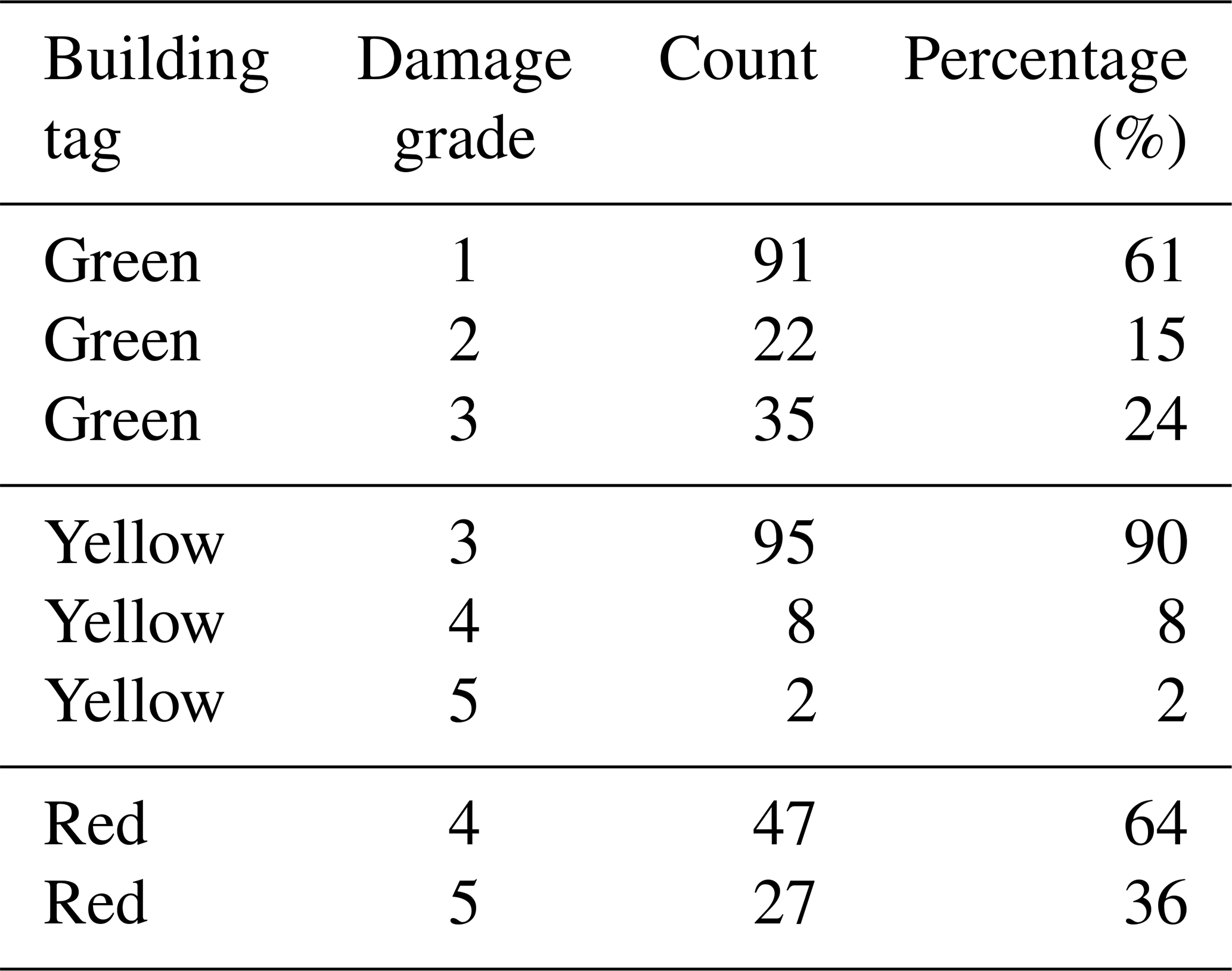
For the conversion of the post-seismic emergency assessments to EMS-98 damage grades, we used the rules in Table 1. We defined these rules based on expert judgement, and they are based on the observed structural and non-structural damage, which is the criterion for classification according to the EMS-98 damage scale. Therefore, for this specific purpose, the essential data in the forms are the entries in the fields for the structural elements bearing vertical and horizontal loads (which were considered separately) and for the non-structural elements as well. The rest of the fields on the forms are related to procedures for life safety, e.g. evacuation, and they were not required for classifying damage according to EMS-98. In this way, we used the raw information from the inspection forms to classify buildings according to structural damage and not whether a building was usable or not. In the cases where a given parameter is red, the damage grade is assigned irrespective of the other parameters. As far as the column “Types of elements” in Table 1 is concerned, the four components are ordered hierarchically. If both vertical and horizontal structural elements are red, then damage grade 5 is assigned, but if the horizontal structural elements are red and the vertical are yellow or green, then grade 4 is assigned. In the cases where everything is green, damage grade 1 is assigned (damage grade 1 corresponds to no structural damage and slight non-structural damage). This assignment is done based on our judgement. The dataset that we used contains only damage observations that were made during inspections on request by the building owners. We assert that at least slight non-structural damage was the cause that led the owners to request an inspection of their building. The results of this reclassification (which involves the distribution of EMS-98 damage levels among the green, yellow, and red tags) are presented in Table 2 for the entire dataset, independently of building typology.
Table 1Proposed classification of the observed damage according to the EMS-98 damage grades as a function of the colour tags assigned by the inspectors.
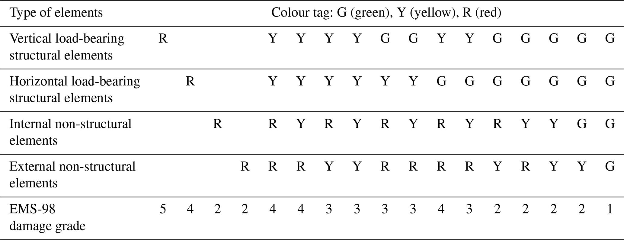
Table 2Percentage of buildings in each damage grade as a function of the building's final tag for the entire dataset.
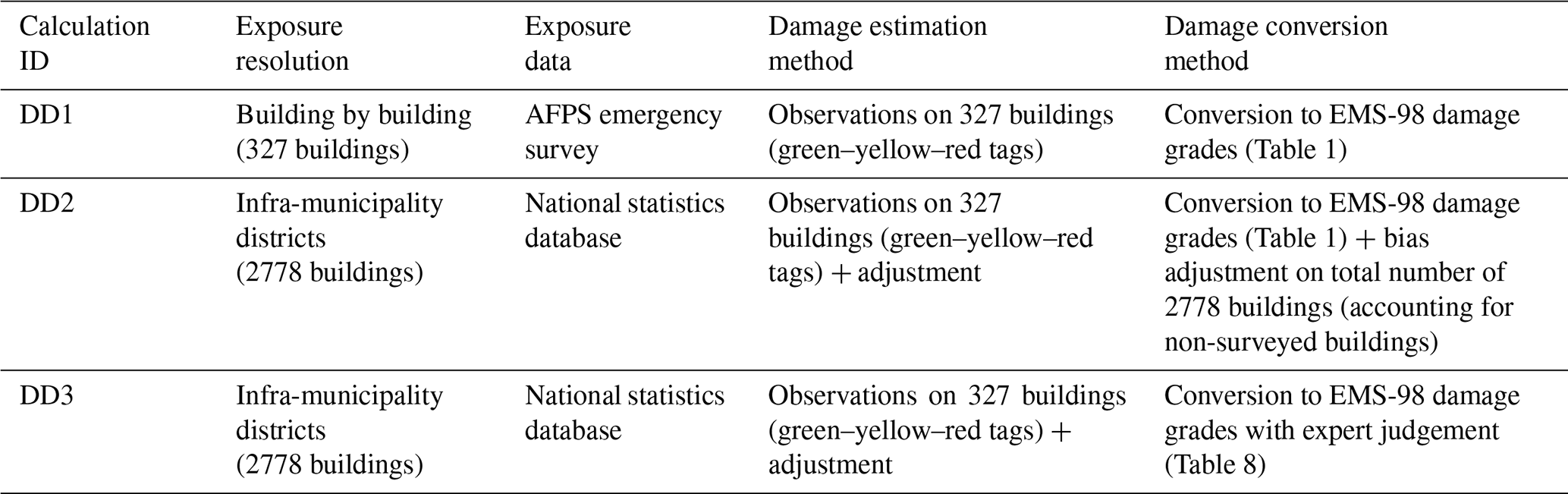
In the following sections, we will compare results of calculations against three different sets of damage distributions that are based on the post-seismic emergency assessments. An overview of the estimation of the three different sets is given in Table 3. The first set, labelled DD1, consists of EMS-98 damage grades resulting from the conversion based on the post-seismic emergency assessments (with respect to the 327 inspected buildings) by applying the rules from Table 1. The damage distributions in DD2 and DD3 are estimated for the entirety of the 2778 buildings in Le Teil (according to the national statistics database): to this end, an adjustment of the distribution in DD1 is performed by applying probabilities of damage grades given the inspection or not of the building in order to account for the fact that only some of the buildings in Le Teil have been inspected.
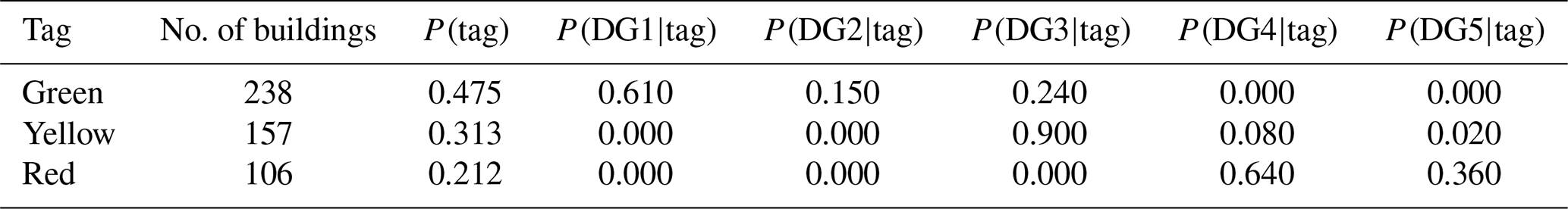
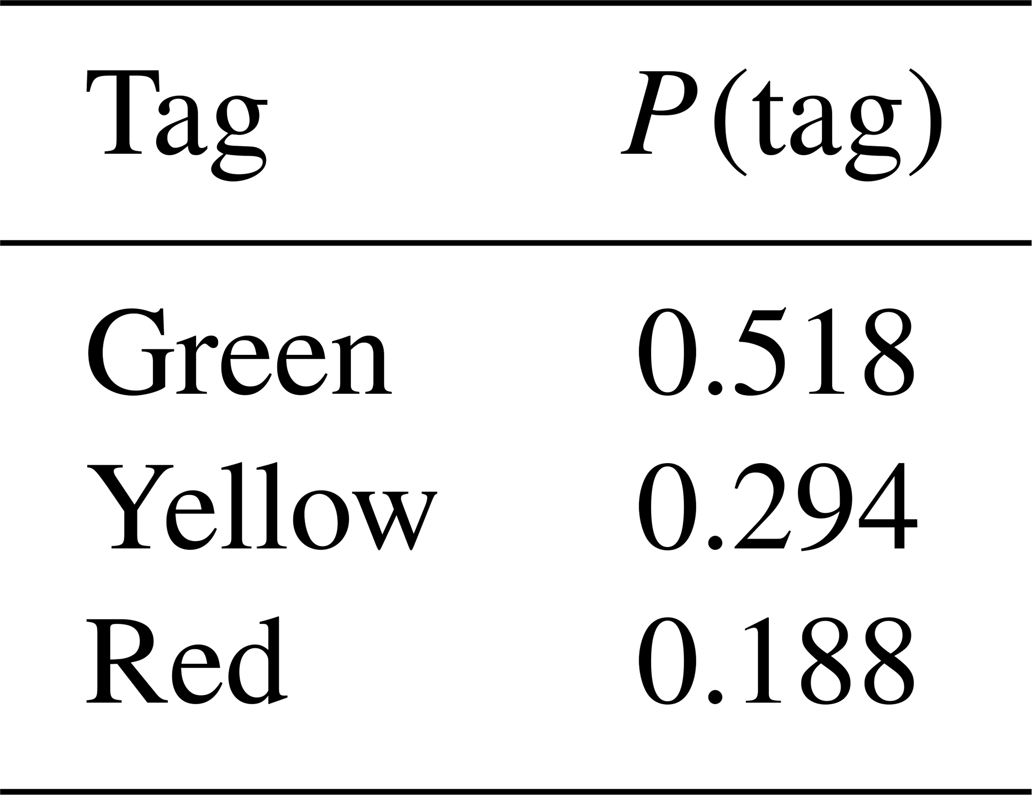
The calculation of the probabilities of the damage grades for DD2 are given in Tables 4 to 7. Table 4 includes the probabilities of the colour tags in the original dataset for 501 buildings. Table 4 also includes the probabilities of the damage grades conditioned on the colour tags that result from the conversion of the post-seismic emergency assessments (Table 2). In Table 5, the total probabilities of the damage grades are calculated assuming that the probabilities of the damage grades conditioned on the colour tags are representative of the 501 buildings in the original dataset. Table 6 gives the damage grade probabilities conditioned on whether a building has been inspected. The first line of Table 6 includes the probabilities based on the damage observations, while the second line includes probabilities of the damage grades for the uninspected buildings, which were selected based on our judgement and our assumption that the damage grade probabilities for the buildings that have not been inspected are different because the inspections were made upon owner request. The probabilities selected for the buildings that have not been inspected are based on our assumption that the probabilities of damage grades 3–5 are significantly smaller than for the inspected buildings. Moreover, we make the assumption that all buildings are at least of damage grade 1. We consider this assumption to be reasonable with respect to the inspected buildings, and we acknowledge that it is conservative in the case of uninspected buildings. In the case of inspected buildings, given that the inspections were made upon request by the owners, we consider the reason behind the requests to be the existence of at least non-structural damage. Furthermore, we consider this assumption to not be excessively conservative given that a large portion of the building stock in Le Teil comprises masonry buildings, in which non-structural cracks are commonly encountered and whose cause is difficult to determine. The calculation of the total probabilities of the damage grades for inspected and uninspected buildings is given in Table 7. Given that these probabilities are practically the probabilities in Table 6 weighted by the probability of a building to have been inspected (, they depend to a large degree on the probabilities for the uninspected buildings because most of the buildings were not inspected (.
Table 4Probabilities of the damage grades conditioned on the colour tag assigned to a building that has been inspected during post-seismic emergency assessments.
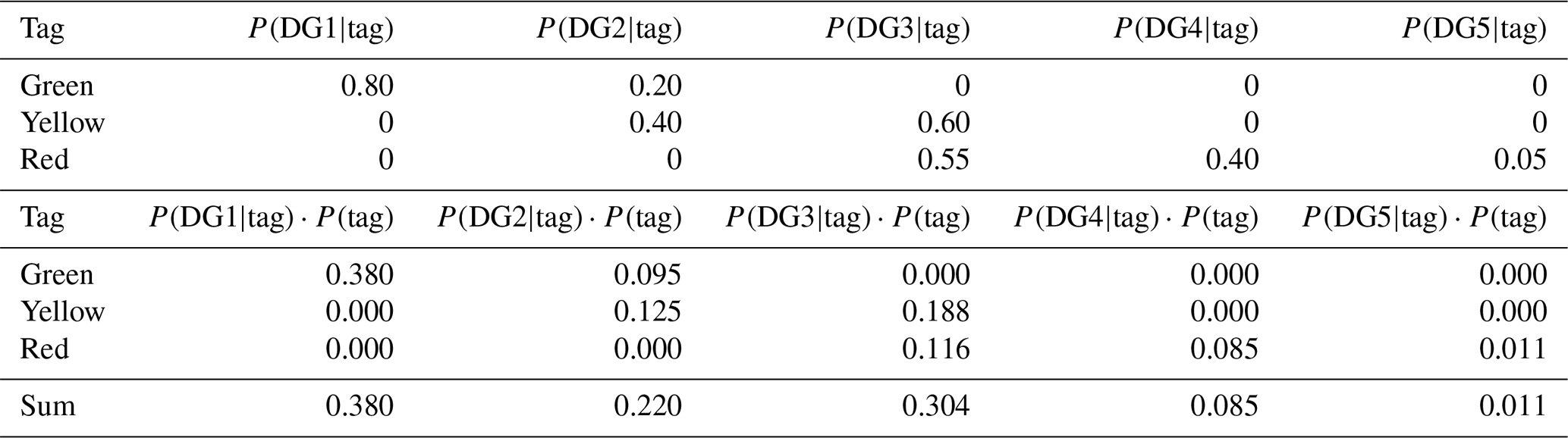
As far as the probabilities for DD3 are concerned, they are calculated using Table 8 in combination with the probabilities of the green–yellow–red tags (P(tag) in Table 4). Specifically, they result if we take a one-row vector of the values in P(tag) in Table 4 and perform a matrix multiplication with the values in Table 8. This calculation differs from the calculation of the probabilities in DD2 in that it implies that the damage observations are representative of the damage over the entire town of Le Teil. This is implied by the fact that there is no conditioning on whether a building has been inspected. The probabilities in Table 8 reflect the judgement of experts who participated in the post-seismic emergency survey in Le Teil. Note that these probabilities may only be applied to this particular earthquake and should not be generalized.
Table 5DD1 calculation of the total probability of the damage grades for buildings inspected during the post-seismic emergency assessments.
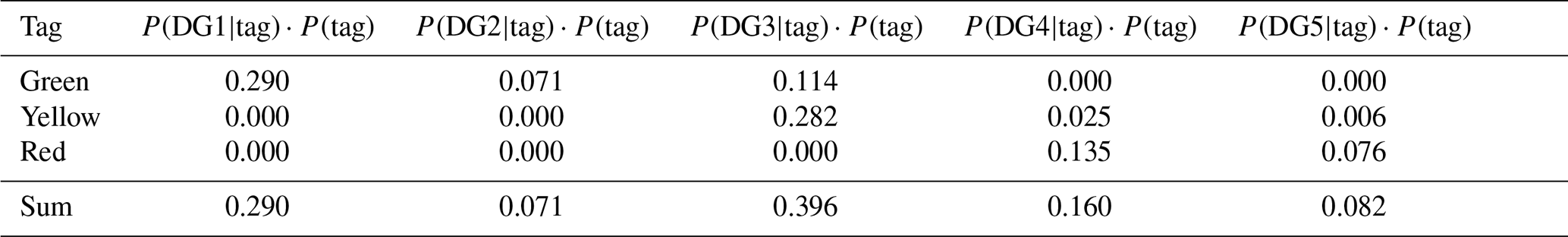
Table 6Probabilities of the EMS-98 damage grades conditioned on whether a building has been inspected (the probabilities for inspected buildings are based on the damage observations, the probabilities for the uninspected buildings are based on expert judgement).
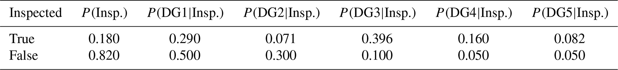
Table 7DD2 calculation of the total probabilities of the EMS-98 damage grades accounting for both inspected and uninspected buildings.
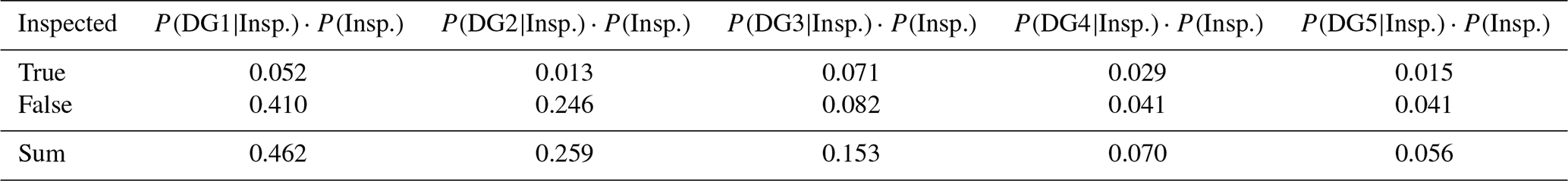
Table 8Probabilities of EMS-98 damage grades conditioned on the building colour tag according to expert judgement and DD3 calculation of the total probabilities of the ESM-98 damage grades.
3.1 Rupture models
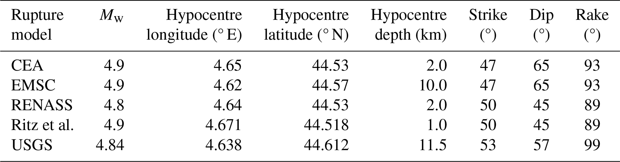
Various ground motion scenarios are generated for different assumptions of rupture models, which are detailed in Table 9. The scenarios are named after the source of the data for the magnitude and the hypocentre location, i.e. CEA (CEA/LDG, 2011; Duverger et al., 2021), EMSC (EMSC, 2019), RENASS (Schlupp et al., 2022), Ritz et al. (Ritz et al., 2020), and USGS (USGS, 2019). The strike, dip, and rake angles of the focal mechanism solutions reported by CEA and Ritz et al. are arbitrarily assigned to the scenarios EMSC and RENASS, respectively. The surface of the rupture is estimated using the Wells and Coppersmith (1994) scaling relation, and the coordinates of the points defining the rupture geometry are calculated in order to be used in the OpenQuake Engine simulations and in the conversion of ground motion IMs to macroseismic intensity. In the case of the rupture model according to the parameters based on Ritz et al. (2020), the area of the rupture model is equal to 6.49 km2. To calculate the coordinates of the corners of the rupture geometry, we assume that its geometric centroid is located at the hypocentre. This assumption leads in some cases to an upper rupture edge above the ground surface. This is amended by translating the rupture geometry on its plane so that its upper edge coincides with the fault trace on the ground surface. The depths of the upper and lower edges of the rupture geometry are used to define the upper and lower seismogenic depths, respectively, in the simple fault model. The coordinates of the ends of the trace of the fault on the ground surface required by the simple fault model are calculated by projecting the rupture geometry on the ground surface in the direction of the dip. Moreover, a maximum rupture mesh spacing of 0.5 km is used, which leads to a 6-by-6 grid in all scenario calculations, which we consider sufficient.
Table 9Rupture parameters associated with the five source models.
3.2 Exposure and fragility models
Regarding the components, three different exposure models are considered in order to characterize the built area of Le Teil. A main distinction is made between aggregated models (i.e. the distribution of building classes within a geographical unit) and models at the level of single buildings.
The first aggregated exposure model (ESRM20 exp.), which is based on the ESRM20 exposure model (Crowley et al., 2019, 2020, 2021b), consists of a single area containing a total of 1679 residential buildings. This exposure model results from a simplification of the ESRM20 exposure model, by fusing similar building types with a small portion of the overall number of buildings in the original ESRM20 exposure model (Table A1) into seven building classes (Table A2). Given that the original ESRM20 exposure model includes classes with a small percentage of the total number of buildings, which could be grouped with similar classes, we opted for such mergers in order to reduce the total number of classes and simplify the comparisons. For example, in Class 1 (Table A1), we decided to group building categories with six or more storeys that have a small number of buildings together with buildings with three–five storeys on the basis of the similarity of their lateral load-bearing systems. The effect of the simplification of the ESRM20 model is checked with an additional calculation using the original ESRM20 exposure model and the corresponding fragility models.
The second aggregated exposure model (BRGM exp.; BRGM is the French Geological Survey) is based on national statistical data, and it includes nine distinct areas (Fig. 2) with 2778 residential buildings. In this exposure model, the buildings are categorized into 12 ESRM20 classes (Table A3), which we selected based on the exposure model in Sedan et al. (2013).
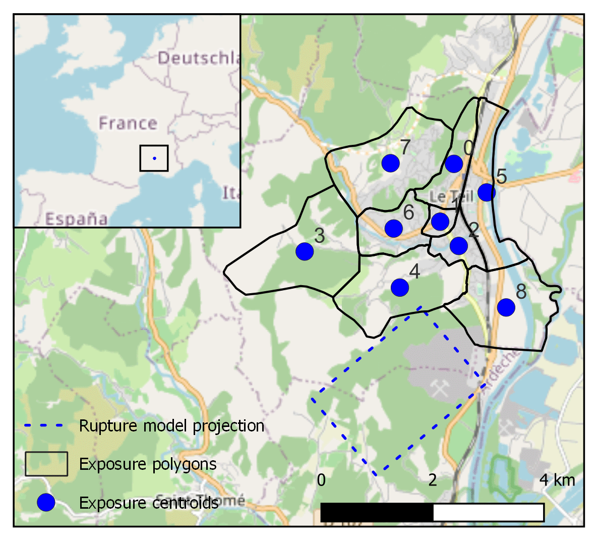
Figure 2Location of the nine exposure centroids in the BRGM exposure model and surface projection of the “Ritz et al.” rupture model (the map includes an OpenStreetMap layer (© OpenStreetMap contributors 2017, distributed under the Open Data Commons Open Database License (ODbL) v1.0)).
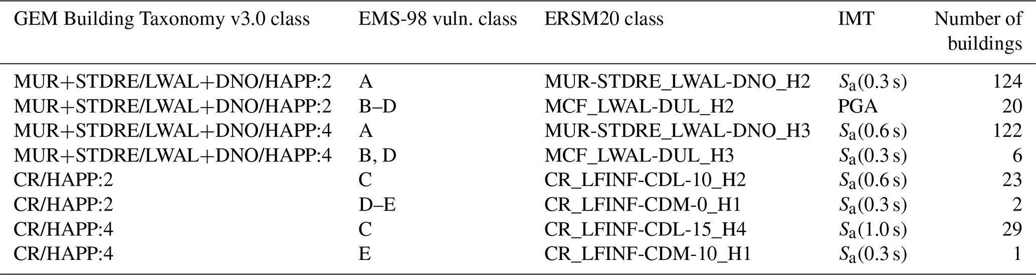
Finally, the building-by-building exposure model includes 327 buildings located at the coordinates of the buildings in the damage dataset DD1, for which the information in the dataset is sufficient for determining the building class and damage grade. In the simulations, the fragility model consists of fragility curves from ESRM20, which we selected according to the information in the damage dataset. Initially, we defined building classes in terms of the GEM Building Taxonomy v3.0 (Silva et al., 2022) based on the building materials and the number of storeys (Table 10). Moreover, we assigned an EMS-98 vulnerability class according to the building material and the year of construction, as well as the building types in Le Teil and their vulnerability class reported by Schlupp et al. (2022). Based on the building type and the vulnerability class, we then selected fragility models from ESRM20. It is noted that the lateral force coefficient could have been estimated based on the date of construction according to Crowley et al. (2021c) but was not considered. Moreover, it was not considered during the selection of the fragility models.
Table 10Assigned GEM Building Taxonomy v3.0, ESM-98 vulnerability, and ESRM20 building classes for the buildings in the post-seismic emergency assessment dataset. The fragility curves in ESRM20 for the selected classes are a function of the listed intensity measure types (IMTs).
3.3 Ground motion models and site amplification
In order to generate the ground motion fields in the scenario calculations, we use two GMMs in the OpenQuake Engine named KothaEtAl2020Site (GEM Foundation, 2023a; a version of the GMM by Kotha et al., 2020, with a polynomial site amplification as a function of the VS30), and KothaEtAl2020ESHM20SlopeGeology (GEM Foundation, 2023b). The GMMs KothaEtAl2020Site and KothaEtAl2020ESHM20SlopeGeology are based on site amplification modelling as a function of VS30 and as a function of slope and geology, respectively. The effect of the VS30 mapping on the estimated probabilities of the damage grade is investigated using two different site models, which are described below.
The first site model (BRGM VS30) uses a map of Eurocode 8 (European Committee for Standardization, 2004) site classes, which was assembled at BRGM for the French territory (Monfort and Roullé, 2016). This map of soil classes was then converted into a VS30 map by taking the median value of each soil class. The resolution in the BRGM VS30 model is based on a geological map at the scale. VS30 values are then directly extracted at the coordinates of the entries in the exposure model, i.e. the nine centroids in the BRGM exposure model, the one centroid in the ESRM20 exposure model, or the 327 points in the building-by-building exposure model.
The second site model (ESRM20 VS30) uses the values of VS30 that are returned for the coordinates of the exposure centroids by the point workflow in the exposure to site tool in ESRM20 (Dabbeek et al., 2021). In the case of the building-by-building scenario calculations, the VS30 values for the ESRM20 VS30 model are obtained using the exposure to site tool in ESRM20, in which the point workflow is applied, which returns the VS30 value associated with the 30 arcsec cell where the query points are found. In addition to the VS30 values, the exposure to site tool returned the type of geology and the slope, which are used subsequently in combination with the GMM KothaEtAl2020ESHM20SlopeGeology.
The VS30 values from the two site models at the coordinates of the centroids in the BRGM exp. exposure model are compared in Table 11. Both site models (BRGM VS30 and ESRM20 VS30), when used in combination with the exposure model BRGM exp., consider one point for each exposure centroid that has identical coordinates to its corresponding exposure centroid. The BRGM VS30 model includes VS30 values corresponding to soft soils, while the lowest VS30 values in the ESRM20 VS30 model are typical of hard-soil sites. The same applies to the VS30 values for the two site models when they are used in combination with the ESRM20 exposure model (Table 12).
Table 11Site parameters in the site models ESRM20 VS30 and BRGM VS30 used in combination with the BRGM exposure model (nine centroids).
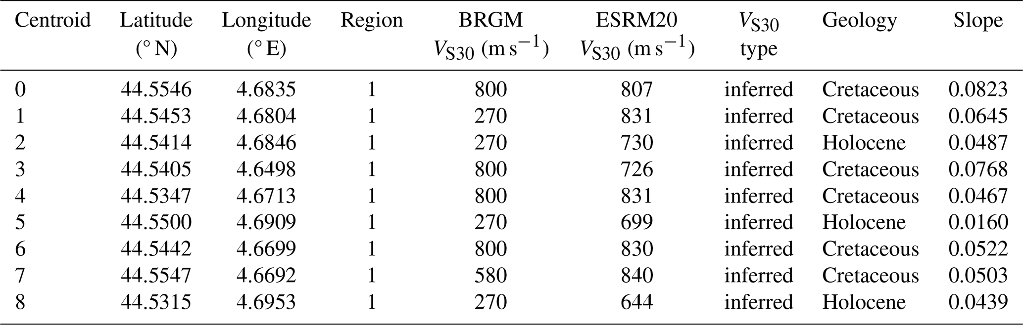
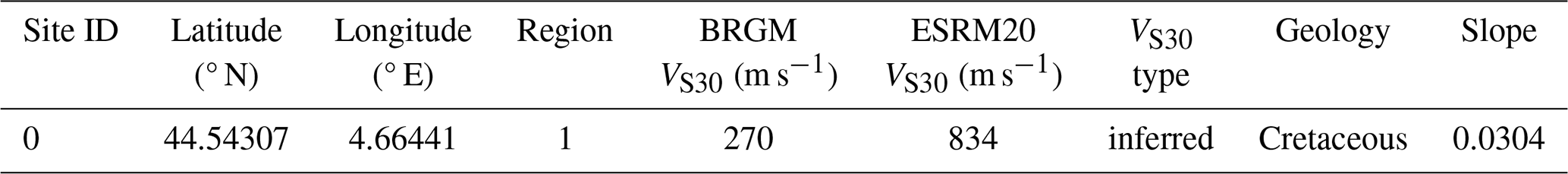
Table 12Site parameters in the site models ESRM20 VS30 and BRGM VS30 used in combination with the ESRM20 exposure model (one centroid).
4.1 Comparison based on ground motion parameters
Here we compare intensity measures of the seismic ground motion resulting from scenario calculations and one shake-map derivation. The scenario calculations are conducted for five different rupture models using the OpenQuake Engine (Pagani et al., 2014; Silva et al., 2014), the ground motion model (GMM) KothaEtAl2020Site, and the BRGM VS30 site model. The geometries of the ruptures in the shake map as well as in the scenario calculations are all modelled as simple faults of flat square geometry, each defined by the set of parameters in Table 9. As far as the shake map for this scenario is concerned, it was re-calculated with the USGS ShakeMap v4 engine (Wald et al., 2022), using the rupture parameters according to Ritz et al. (2020) (i.e. Ritz et al. model in Table 9), and it was constrained with ground motion measurements only (no “did you feel it?” reports were used). However, the closest stations are over 15 km from the epicentre, which leads to practically no constraint.
To account for the uncertainty in the intensity of the ground motion, 1000 ground motion fields are generated, i.e. samples of IMs at the location of the nine centroids of the aggregated exposure model. The ground motion fields are generated by the OpenQuake Engine for the IM peak ground acceleration (PGA), with spectral pseudo-acceleration at 0.3, 0.6, 1.0, and 3.0 s. Furthermore, the spatial correlation of the IMs is taken into account in the generation of the IM samples using the Jayaram and Baker (2009) model in the OpenQuake Engine, assuming no clustering of the VS30 values in the study area. As far as the correlation between spectral periods is concerned, the default correlation model BakerJayaram2008 by Baker and Jayaram (2008) is used by the OpenQuake Engine.
On the other hand, the shake-map estimates parameters of the lognormal distributions of the IMs (PGA, spectral acceleration at 0.3, 0.6, and 1.0 s) at the nine centroids, which are then used to generate ground motion fields, i.e. 1000 samples for each IM at each centroid, using R (R Core Team, 2023). For the generation of the samples, we use our implementation of the correlation models for the spatial correlation (Jayaram and Baker, 2009) and the correlation between spectral accelerations at different periods (Baker and Jayaram, 2008), as in the calculations with the OpenQuake Engine. Based on the correlation models, we define a symmetrical correlation matrix containing one row (and one column) for each spectral period at each site. The sites are defined based on the coordinates of the exposure centroids (in Sect. 5.1, the sites are defined using the coordinates of the individual buildings in the case of the calculations using the building-by-building exposure). Additionally, for the sampling, we use the nearest positive definite matrix and the approach by Higham (2002) as implemented in the R package Matrix (Matrix package authors and Oehlschlägel, 2023) in order to overcome the problem of a non-positive definite correlation matrix. The sampling is performed using the R package faux (DeBruine, 2023).
Figure 3 shows box plots for the samples of the considered IMs, which were generated at the locations of the exposure centroids. For a specific IM, the median and the mean of the entirety of the samples for all centroids are represented by the line at the middle of the box and the point marker, respectively. The boundaries of a box mark the first and third quartile, while the whiskers approximate the 95 % confidence interval. If we consider only the box plots corresponding to the five scenario calculations, the dispersions of the samples are equivalent, as expected due to the use of the same GMM. However, the differences with respect to the means of these five IM samples have to be attributed to the differences between the epicentre locations, the depth of the hypocentre, and the focal solution because these are the parameters affecting the distance between the exposure centroids and the geometry of the rupture. Moreover, the means for the scenarios EMSC and USGS are consistently the lowest. We attribute this primarily to the hypocentral depths in these two scenarios (10.0 and 11.5 km), which are significantly larger than those in the other three scenarios, leading to distances from the rupture of between 10.0 and 25.0 km, whereas the corresponding distances in the other three scenarios are less than 5.0 km. Regarding the samples based on the shake-map derivation, the box plot whiskers are relatively short compared to those for the five scenarios, signifying smaller dispersions of the IM logarithms. This difference should primarily originate from the differences between the GMMs in the shake-map configuration and in the scenario calculations.
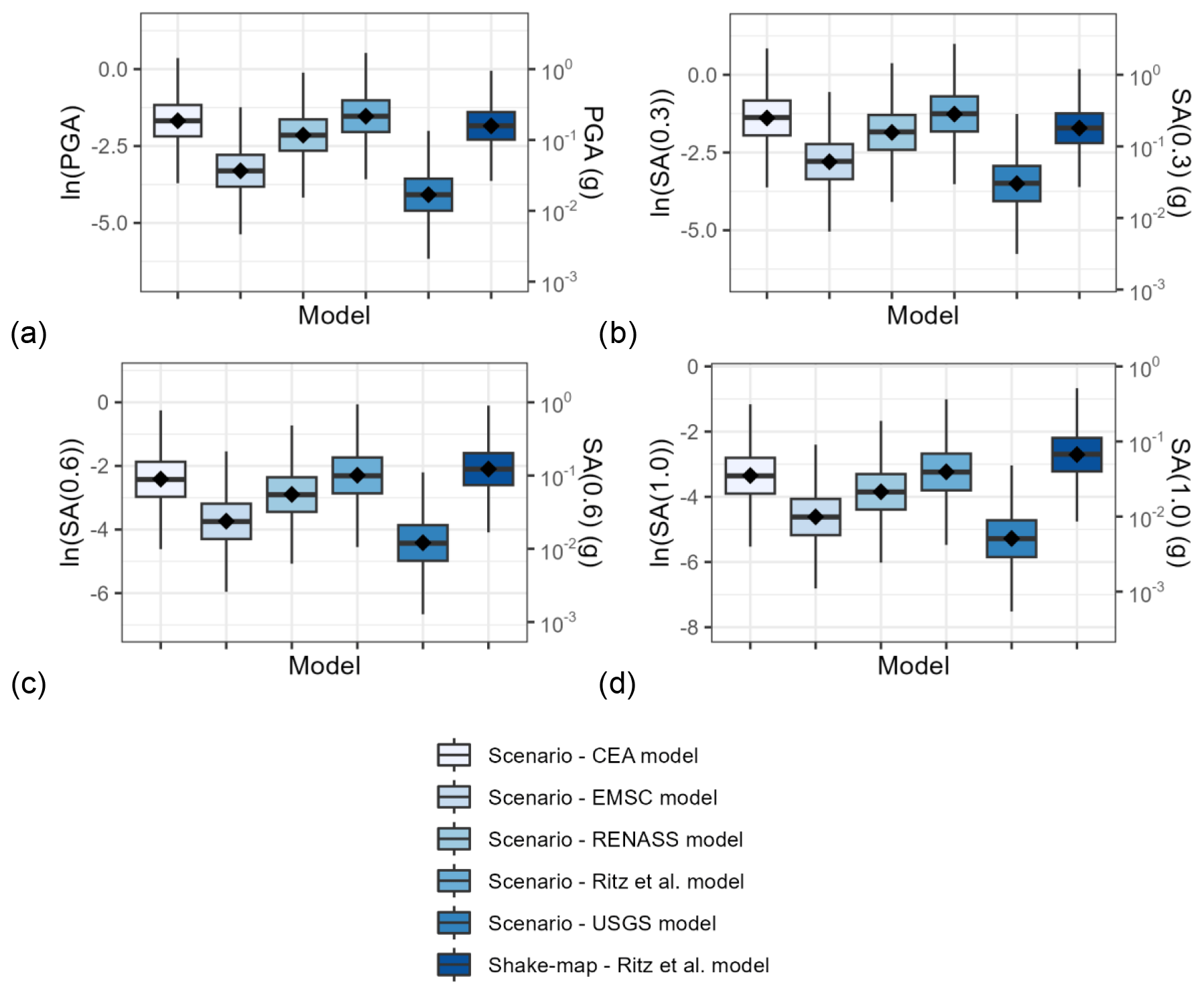
Figure 3Ground motion intensity measures aggregated from all exposure centroids (the edges of the box are located at the first and third quartile, respectively; the line at the middle of the box is located at the median; the point marker is located at the mean of the sample; the whiskers extend up to 1.5 times the distance between the first and third quartile, approximating the 95 % confidence interval).
4.2 Comparisons based on macroseismic intensity
The generated IM samples are subsequently converted to macroseismic intensities using GMICEs, and they are compared with the macroseismic intensity reported by Schlupp et al. (2022). The aim of this comparison is to identify the rupture models leading to macroseismic intensities closest to the reported ones. Moreover, another motive for this comparison is the fact that it is difficult to compare the models with measured observations (i.e. recordings of seismic stations), since such measures are very sparse (the nearest station is around 15 km from the epicentre). Therefore, in the absence of measures in the epicentral area, it is difficult to compare the effects of different rupture distances in this area to measured ground motions (this is where the relative differences in rupture distance are the largest, as they are greatly reduced further away from the epicentre). This is why we use macroseismic intensity (precise estimates obtained from field surveys) for the comparison. Two GMICEs are used for this comparison, which we consider compatible with the study area. These are the GMICEs by Faenza and Michelini (2010) (Eq. 1) and by Caprio et al. (2015) (Eq. 2).
where MCS is the Mercalli–Cancani–Sieberg intensity, IM is PGA (in cm s−2) or PGV (peak ground velocity; in cm s−1), and σ is the model's standard deviation.
where INT is a combination of the Modified Mercalli Intensity (MMI) and the Mercalli–Cancani–Sieberg intensity (MCS); IM is the ground motion intensity measure, i.e. PGA (in cm s−2) or PGV (in cm s−1); a and b are the model's parameters; and σ is the model's standard deviation. The Caprio et al. (2015) model is bilinear, and its parameters are found in Table 13, while the Faenza and Michelini (2010) model is the single-line model in Faenza and Michelini (2010), whose parameters are found in Table 14. To account for model uncertainty during the conversions with Eqs. (1)–(2), random residuals were generated from zero-centred normal distributions with the corresponding standard deviation and added to the means given by the equations.
Table 13Parameters used in the implementation of the model by Caprio et al. (2015).
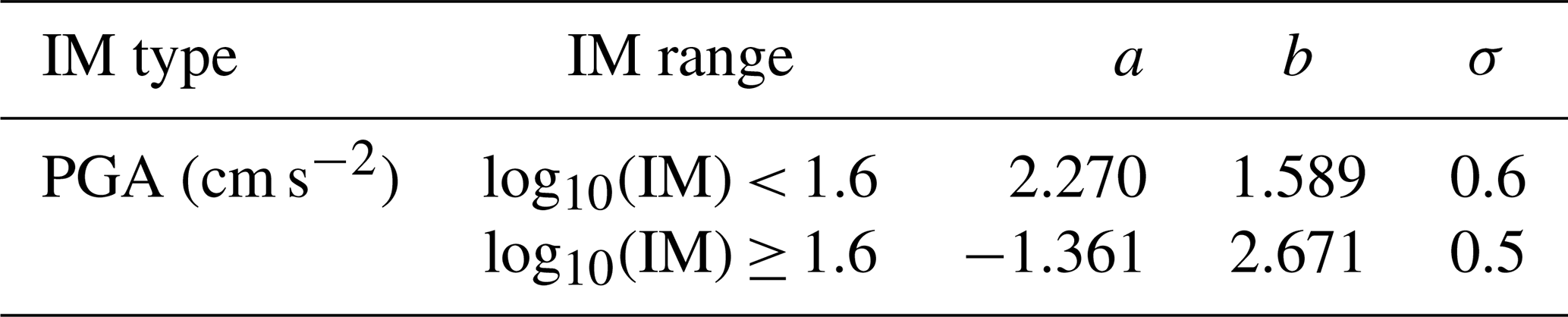
Table 14Parameters used in the implementation of the model by Faenza and Michelini (2010).
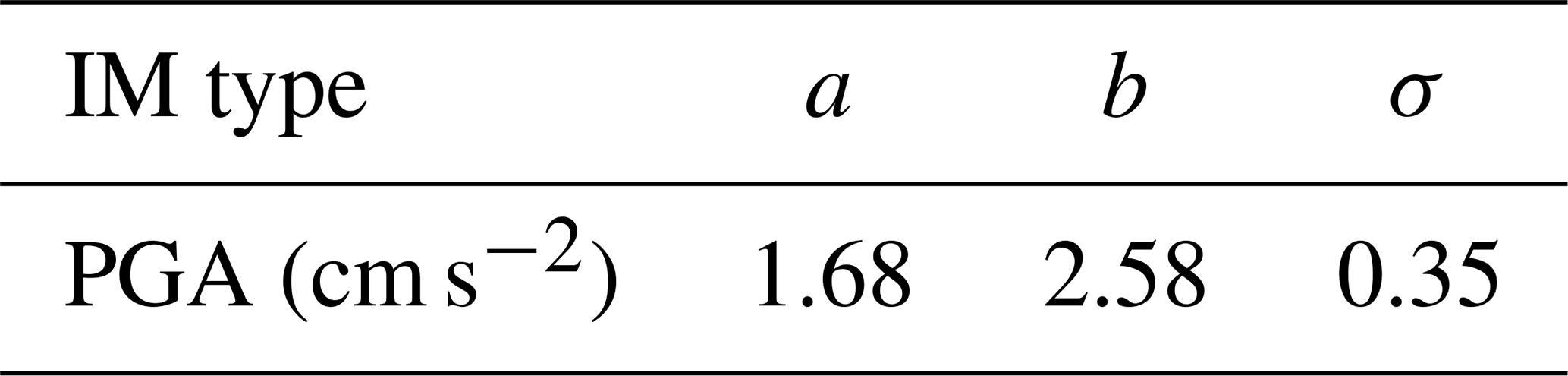
Figure 4 shows the box plots for MCS and INT, respectively, which result from the conversion of the IM samples. Despite the fact that MMI and MCS have differences, here we adopt the guidelines by Musson et al. (2010), which take the two scales as equivalent (to each other and to the EMS-98 scale) up to intensity 10. We make this assumption to distinguish the effects of the employed GMICEs on the distributions of the generated samples of macroseismic intensities in Fig. 4 from the differences due to the underlying hazard model components.
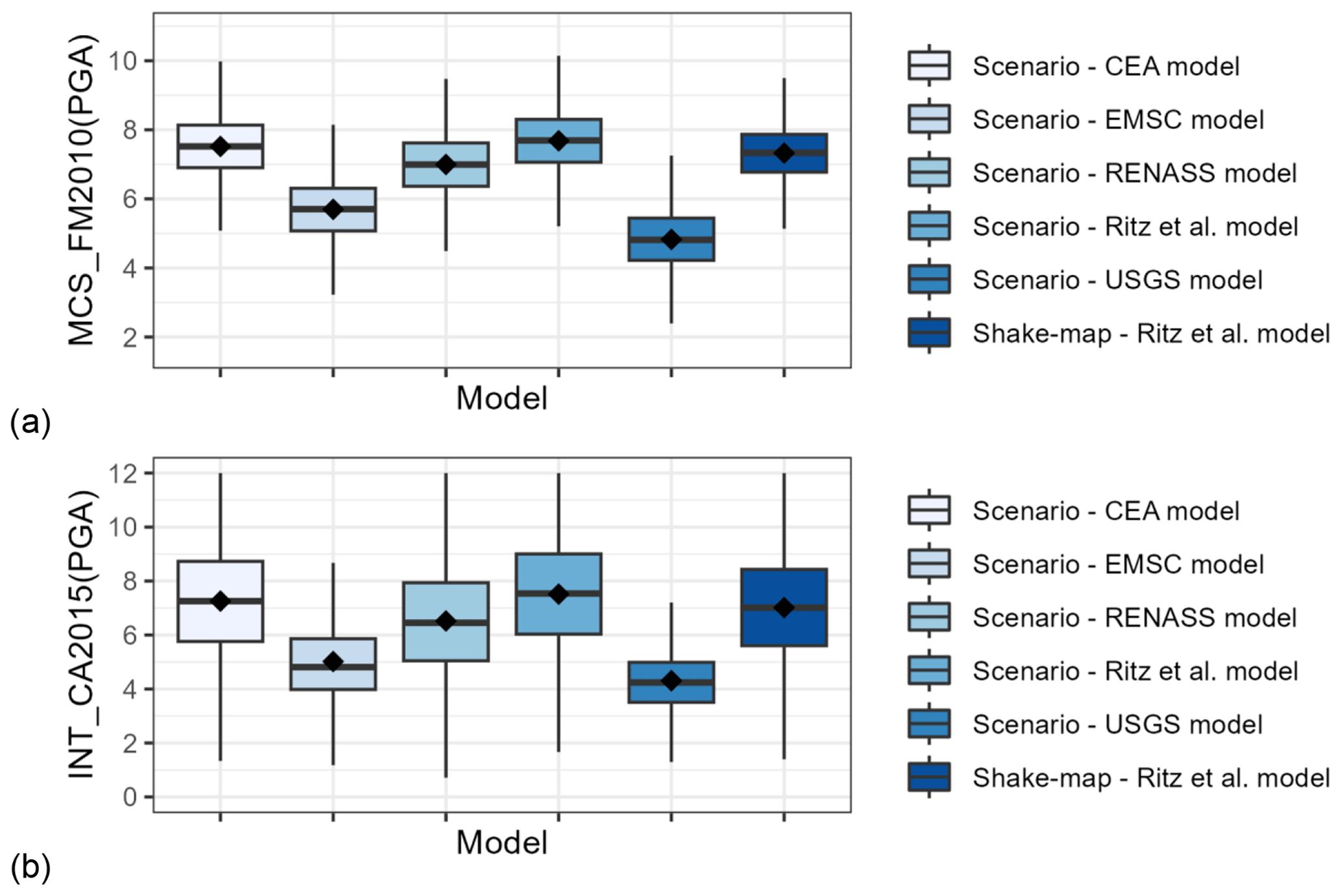
Figure 4Box plots for (a) the Mercalli–Cancani–Sieberg (MCS) macroseismic intensity as a function of the PGA given by the ground motion-to-intensity conversion equation by Faenza and Michelini (2010) (FM2010) and (b) the macroseismic intensity (INT) as a function of the PGA given by the ground motion-to-intensity conversion equation by Caprio et al. (2015) (CA2015) (the edges of the box are located at the first and third quartile, respectively; the line at the middle of the box is located at the median; the point marker is located at the mean of the sample; the whiskers extend up to 1.5 times the distance between the first and third quartile, approximating the 95 % confidence interval).
In order to assess the usefulness of the distribution for each scenario in Fig. 4, we are using the 7.5 EMS-98 intensity estimated by Schlupp et al. (2022) for the municipality of Le Teil. The MCS distributions resulting from the Faenza and Michelini (2010) model, whose median is closer to the 7.5 observation-based estimation, are those for the CEA, RENASS, and Ritz et al. scenarios, as well as the shake-map derivation. As far as the application of the Caprio et al. (2015) model (Fig. 4b) is concerned, it leads to macroseismic intensity distributions with larger dispersions and lower medians compared to the distributions calculated using the model by Faenza and Michelini (2010) (Fig. 4a) in the cases considered. In the cases examined here, the distributions whose medians are closest to the 7.5 observation-based estimation are those from the scenarios CEA, RENASS, and Ritz et al. and from the shake map. Based on this, the Ritz et al. rupture model is used in the calculations that follow.
5.1 Estimated damage based on a building-by-building exposure model
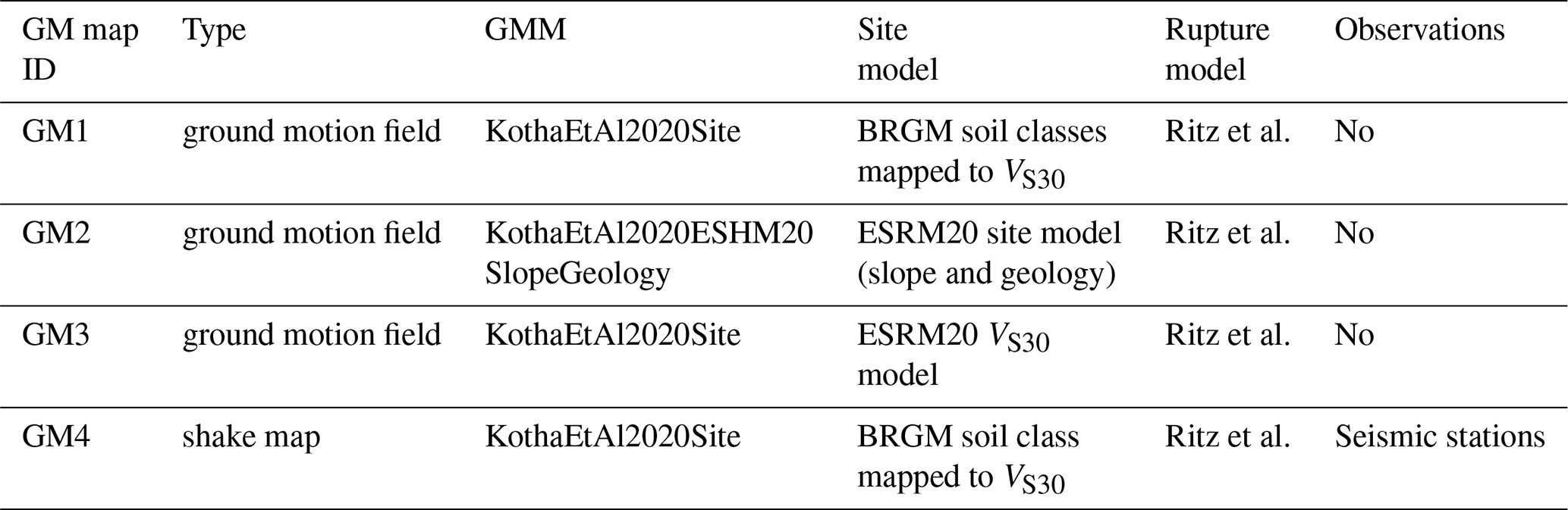
First, we perform scenario damage calculations using the OpenQuake Engine and the building-by-building exposure model, which includes 327 buildings with classes defined in Table 10. The ground motion fields in the calculations are generated using four different configurations (Table 15), which include the two different GMMs, i.e. KothaEtAl2020Site and KothaEtAl2020ESHM20SlopeGeology, and three different site models. In all cases, the rupture is modelled according to the Ritz et al. scenario (Table 9). A scenario calculation is also performed using ground motion fields generated from the shake-map procedure described in Sect. 4.1 as input (GM4 in Table 15).
Table 15The configurations (GM map IDs) used to generate the ground motion fields in the scenario damage calculations based on a building-by-building exposure model.
The damage based on the scenario damage calculations is firstly calculated on the damage scale of the ESRM20 fragility models, and then it is converted to the ESM-98 damage scale using the structural damage according to Table A4 as a criterion. Due to this conversion, all buildings in the calculation have at least non-structural damage. In this case, the building-by-building exposure model includes the inspected buildings, and as discussed in Sect. 2.2, it is reasonable to assume that completely undamaged buildings are underrepresented in the sample of inspected buildings.
Figure 5 gives the distribution of the damage grades and the corresponding number of buildings based on the calculations. First, it is worth noting that the GM4 simulation leads to similar but somewhat lower probabilities for the damage grades 3–5 compared to the GM1 simulation. GM1 and GM4 use the same GMM and site model; the difference lies in the fact that GM4 uses ground motion fields based on a shake map. The main drivers of the probabilities of the damage grades are the buildings in the classes MUR-STDRE_LWAL-DNO_H2 and MUR-STDRE_LWAL-DNO_H3, which include 38 % and 37 %, respectively, of the total number of buildings in the model. These two classes are also the most vulnerable among the classes in the model, as indicated by the fact that they were classified into EMS-98 vulnerability class A. The fragility curves of these two building classes are functions of Sa(0.3 s) and Sa(0.6 s), respectively. Based on the results in Fig. 3, we consider the Sa(0.3 s) to be higher on average in the calculation “Scenario − Ritz et al. model” (GM1) than in “Shake-map − Ritz et al. model” (GM4) and there to be no significant differences between the two with respect to Sa(0.6 s). This is the factor to which we attribute the differences in the probabilities of the damage grades based on the simulations GM1 and GM4.
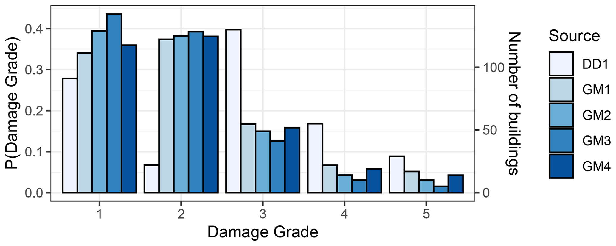
Figure 5Distribution of the damage grades based on the calculations with the building-by-building exposure model compared with the DD1 estimation of actual damage.
The GM3 calculation leads to the lowest probabilities for the damage grades 3–5 amongst all computations in Fig. 5. In this simulation, 68 % of the buildings are located on sites with VS30≥ 800 m s−1, while in GM1 72 % of the buildings are on sites with VS30≤ 360 m s−1, which is expected to lead to higher ground motion intensities due to site amplification. It interesting to note that the GM2 calculation, which uses the KothaEtAl2020ESHM20SlopeGeology GMM, gives results which are practically halfway between the results of the calculations GM1 and GM3.
Figure 5 also includes the estimation DD1 (Table 3) of actual damage, which is based on our conversion of the damage observation. For damage grades 4 and 5, there are significant differences between the probabilities based on DD1 and the probabilities based on the scenario calculations and the shake maps (GM1–4); however, they are not as important as the differences in the case of damage grades 2 and 3. We presume that the rule that we used for the translation of the damage observations to damage grades (Table 1) is the source of these discrepancies. Moreover, DD1 leads to a distribution in Fig. 5 that has an unusual valley for damage grade 2. The proposed mapping of damage observations assigns damage grade 3, when the vertical or the horizontal structural elements have a yellow tag (see Table 1). We believe that a yellow tag with respect to the structural elements signifies moderate structural damage, hence damage grade 3. The fact that in these cases a green tag was assigned (Table 2) perhaps indicates that a further inspection took place which reclassified the damage either as green structural damage or as yellow non-structural damage. Such cases could be taken into account by a future refinement of the proposed mapping scheme.
5.2 Estimated damage based on aggregated exposure models
In addition to the building-by building calculations, we perform a series of scenario damage calculations with the two aggregated exposure models that include the total number of residential buildings in the municipality of Le Teil. In the calculations with the aggregated exposure models, the ground motion intensity measures are modelled with nine different combinations of GMMs, site models, and exposure models, as shown in Table 16.
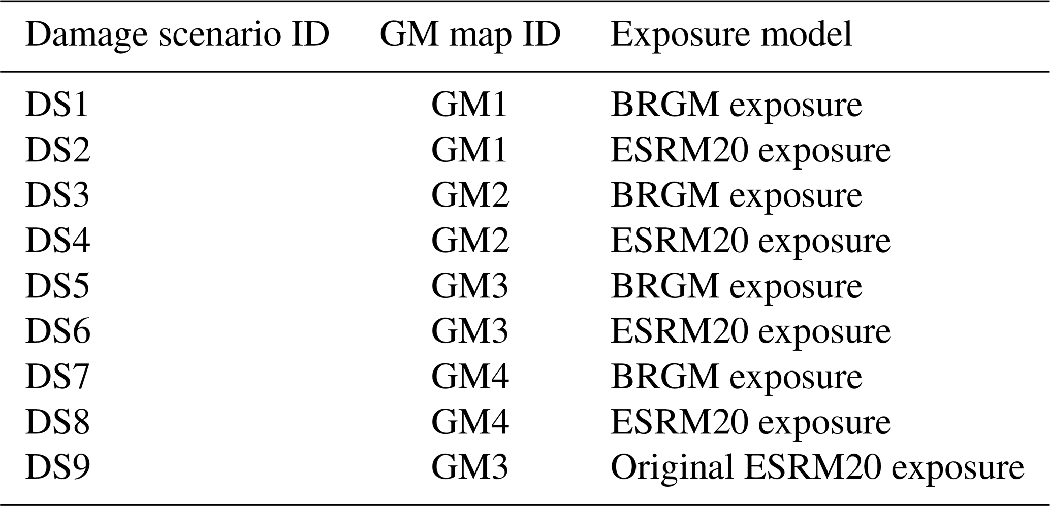
Table 16Combinations of ground motion map IDs with the exposure models for each damage scenario ID.
As in the calculations based on the building-by-building exposure model, the damage based on the scenario damage calculations is converted from the ESRM20 damage grades to the ESM-98 damage grades using Table A4. In this case, this assumption may lead to an overestimation of non-structural damage. However, as discussed in Sect. 2.2, this overestimation may not be excessive due to possible non-seismic pre-existing non-structural damage, especially in masonry buildings, which make up the biggest part of the building stock in Le Teil.
In Fig. 6, we may see the effect of the different exposure models on the distribution of the damage grades and on the corresponding number of buildings. Figure 6a includes the distributions of the damage grades for the damage scenarios DS5, DS6, and DS9, which all use the same rupture model, GMM, and site model (GM3). Compared to DS5, the DS6 calculation for the ESRM20 exposure model leads to somewhat higher probabilities for damage grades 3–5. The differences between DS5 and DS6 are due to the use of the BRGM and ESRM20 exposure model, respectively. Moreover, Fig. 6a includes the results of damage scenario DS9, which uses the original ESRM20 exposure and fragility model to check the effect of the simplification of the ESRM20 exposure and fragility models. By comparing the results between DS6 and DS9, we conclude that the simplification has a minor effect on the results. Figure 6a also includes our estimations DD2 and DD3. The reader is reminded that DD2 depends mostly on expert judgement and on the damage observation to a lesser extent, while DD3 is entirely based on expert judgement (see Sect. 2.2). Note that, in DD3, the probabilities for damage grades 3–5 depend heavily on the probabilities of these damage grades conditioned on a red tag, which were assigned based on expert judgement. In hindsight, it may have been too optimistic to assign a 55 % probability of damage grade 3 in the case of a red tag. In DD3, alternative assignments of the probabilities for a red tag may smooth out the peak for damage grade 3. The probabilities of the damage grades 3 and 4 calculated by the damage scenario calculations DS5, DS6, and DS9 are lower than the DD2 and DD3 estimations. However, for damage grade 5, the results of the damage scenarios are found in the range between the DD2 and DD3 estimations. The same trends may be observed (not shown here) by comparing the calculations DS1 and DS2 (based on GM1), DS3 and DS4 (based on GM2), or DS7 and DS8 (based on GM4).
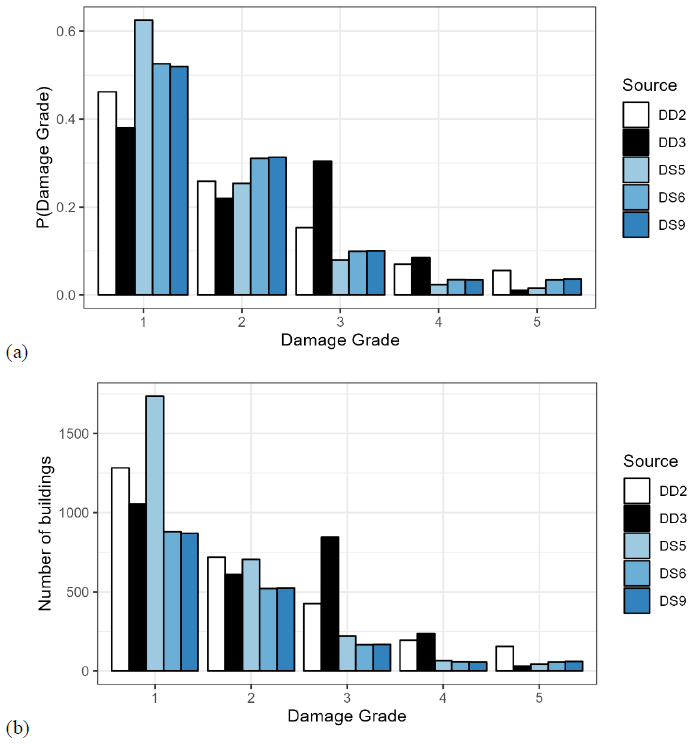
Figure 6Effect of the exposure model on the (a) probabilities and (b) number of buildings per EMS-98 damage grade for the calculations with an aggregated exposure including the total number of buildings in Le Teil.
The numbers of buildings in Fig. 6b are calculated by multiplying the total number of buildings in the exposure model by the probabilities in Fig. 6a. In the case of the DD2 and DD3 estimations, we chose to calculate the number of buildings by multiplying the damage grade probabilities with the number of buildings in the BRGM exposure model. Despite the difference in the total number of buildings in the BRGM and in the ESRM20 exposure models (2778 versus 1679), the results of the damage scenarios for damage grades 3–5 present minor differences.
The comparison with respect to the site amplification models is done using the damage scenario calculations DS1, DS3, DS5, and DS7 (Fig. 7a), where the same exposure model is used, i.e. the BRGM exposure model, but each time we use one of the four different GM maps (GM1 to GM4 in Tables 15 and 16). The effect of using the BRGM VS30 model instead of the ESRM20 VS30 model may be seen by comparing DS1 with DS5. The probabilities of the damage grades 2–5 are slightly lower in the scenario DS5. This may be explained by the fact that the VS30 values are higher in GM3 than in GM1; however we would expect more important differences considering the differences in the VS30 values shown Table 11. The damage grade probabilities in the scenario DS3, which uses the KothaEtAl2020ESHM20SlopeGeology GMM, are between the results for DS1 and DS5 for all damage grades. As far as the results based on DS7, which uses a shake map, they present small differences from those from DS1, which is reasonable considering that they use the same ground motion and site model and that the updating based on ground motion observations in the shake map is minor. The results based on the ESRM20 exposure and fragility model (Fig. 7b) show a similar image with the exception of the difference between DS2 and DS8. Again, DS2 and DS8 use the same ground motion and site model, so the origin of this difference may be found in consideration of observations in the shake map used by DS8.
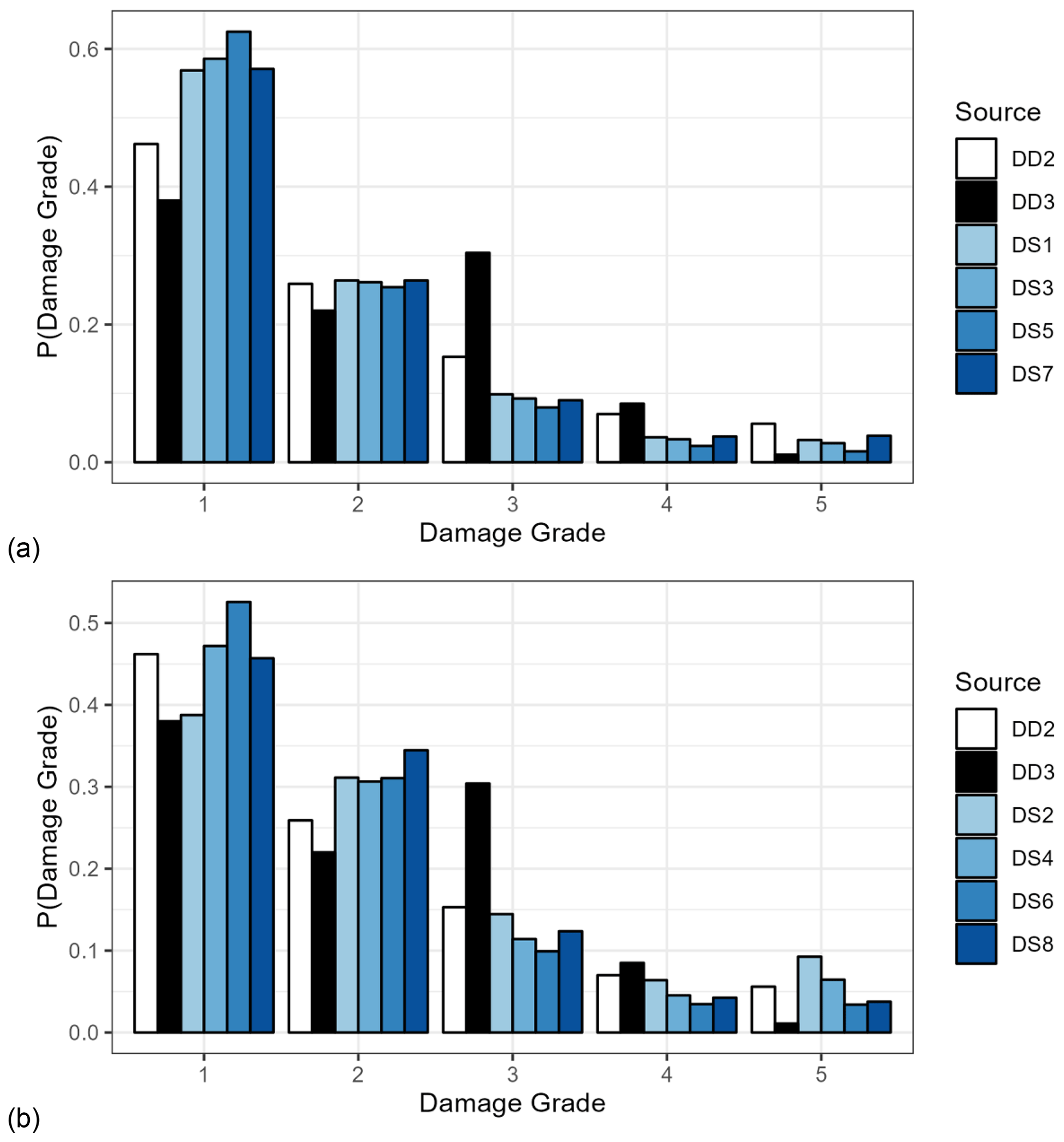
Figure 7Effect of the GMM and site model on the probabilities of the EMS-98 damage grade for the calculations with (a) the BRGM and (b) the ESRM20 aggregated exposure models including the total number of buildings in Le Teil.
5.3 Estimated damage based on a semi-empirical vulnerability approach
For a comparison with respect to the distribution of damage according to different calculation methodologies, we compare the estimated damage using the seismic risk analysis tool Armagedom (Sedan et al., 2013), running on the VIGIRISKS platform (Negulescu et al., 2023), with an estimation made and the DS1 scenario calculation with the OpenQuake Engine.
The Armagedom tool implements the semi-empirical macroseismic method developed by the RISK-UE project (Lagomarsino and Giovinazzi, 2006). In contrast to the scenario calculations with the OpenQuake Engine, where 1000 ground motion realizations are used to account for ground motion uncertainty, the calculation with Armagedom takes a third-party pre-calculated map of macroseismic intensity as input. For the calculation with Armagedom, we use the macroseismic intensity map produced by Schlupp et al. (2022). The semi-empirical macroseismic method applied by Armagedom calculates the mean EMS-98 damage grade as a function of the macroseismic intensity and two parameters, i.e. the vulnerability and the ductility index. These indices have been assigned to building classes in the exposure model used for the calculation using Armagedom based on criteria such as the material and the year of construction (Sedan et al., 2013). Subsequently, the semi-empirical macroseismic method applied in Armagedom assumes a binomial distribution to calculate the probabilities of exceeding the EMS-98 damage grades as a function of macroseismic intensity. On the other hand, the OpenQuake Engine uses ground motion realizations in combination with fragility curves to generate realizations of damage.
The estimated distribution of buildings in each damage grade based on the two calculations is given in Fig. 8, along with the distribution from the damage datasets DD2 and DD3. The percentage of buildings with heavy and very heavy damage is 1.1 % and 0.0 % with Armagedom and 3.7 % and 3.3 % with the OpenQuake Engine, respectively. Both the DS1 calculation and the Armagedom calculation lead to estimations for damage grades 3 and 4, which are lower than the estimations DD2 and DD3. As far as damage grade 5 is concerned, the DS1 calculation estimates a probability of 3.3 %, which lies between the DD2 and DD3 estimations, i.e. 5.6 % and 1.1 %, respectively. On the other hand, the Armagedom calculation globally underestimates damage when compared to the DS1 calculation. It should be noted that DS1 is based on the GM1 map, which corresponds to macroseismic intensity ranges (see Fig. 4) that are well in line with the estimates by Schlupp et al. (2022), i.e. intensity around 7.5. Therefore, differences between DS1 and Armagedom may be mostly attributed to the different methods of damage estimation, i.e. the conversion between building vulnerability classes and corresponding fragility functions.
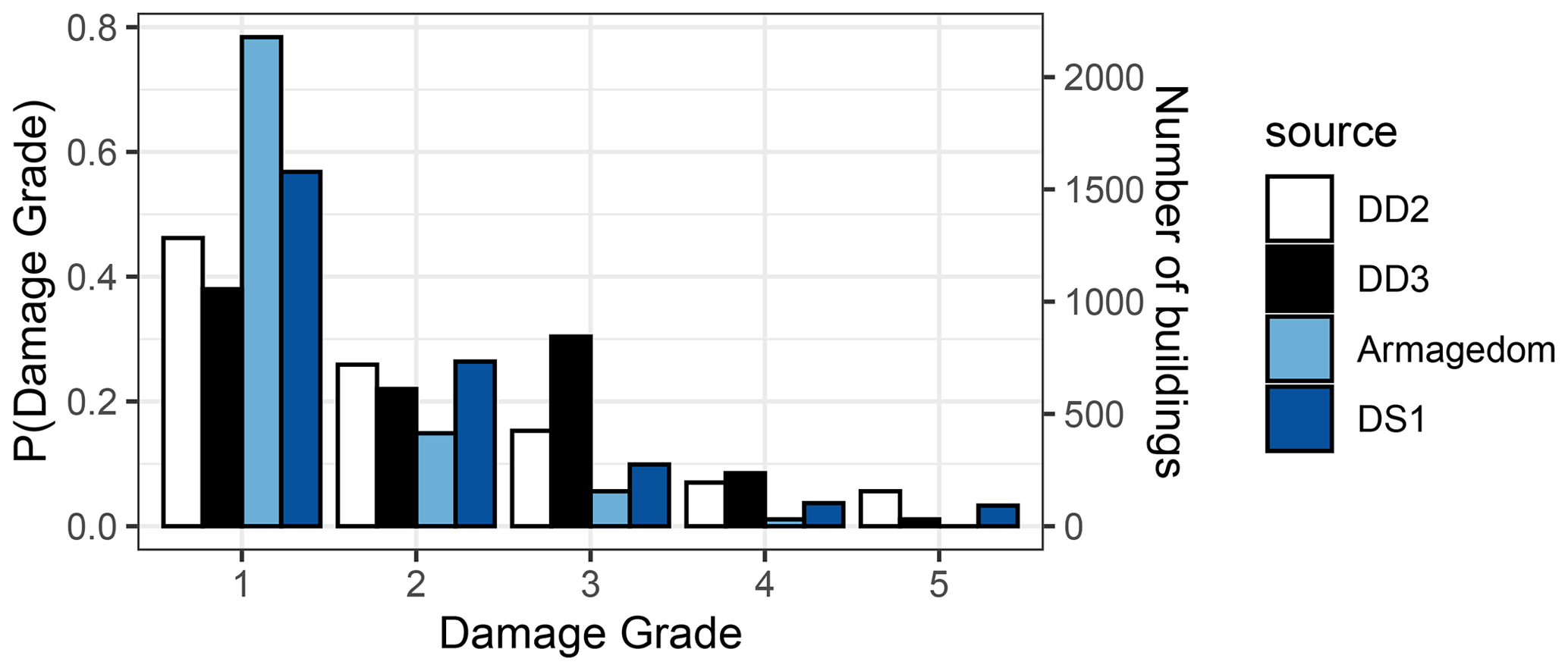
Figure 8Estimation of damage grades using the Armagedom tool compared to the estimations DD2–DD3 and the results of the DS1 calculation.
Using simulations of earthquake scenarios and shake maps, we conducted comparisons based on ground motion intensity, macroseismic intensity, and the estimated amount of damage based on different risk model components. Moreover, we produced a dataset of 327 entries containing damage on the EMS-98 scale based on emergency post-seismic assessments on a three-level (red–orange–green) scale, which were made after the Le Teil 2019 earthquake. The damage on the EMS-98 scale in the dataset is the result of a conversion based on a proposed rule, which considers structural and non-structural damage. The dataset produced was also used to make estimations for the entirety of the residential building stock in Le Teil.
Based on scenario calculations using the OpenQuake engine, as well as shake maps, we calculated the ground motion intensity at a series of points of interest in the town of Le Teil, and then we converted the ground motion intensity to macroseismic intensity. This was done for different models of the earthquake rupture to select the model to be used in subsequent damage scenarios.
The damage scenarios used different ground motion models, site models, and exposure and fragility models to study the effect of these modelling assumptions. The GMMs used are KothaEtAl2020Site and KothaEtAl2020ESHM20SlopeGeology, while the site models include a site model based on VS30 values that, in turn, are based on a map of site classes produced by BRGM and a site model based on ESRM20. As far as the exposure models are concerned, they include the BRGM exposure for Le Teil, a model based on French national statistical data, and the ESRM20 exposure model.
The scenario damage calculations lead to probabilities for damage grades 3–5 based on ESRM20 with small differences from the probabilities based on the BRGM exposure and fragility model. Furthermore, the damage scenarios using the ESRM20 exposure and fragility model are overall in better agreement with the calculations DD2 and DD3 (see Sect. 2.2 for the details of the calculations). In general, the scenario damage calculations estimate lower probabilities for damage grades 3–4 than the DD2 and DD3 calculations using the damage dataset, while they are in better agreement in the case of damage grade 5. The estimation based on the Armagedom tool results in probabilities of damage grades 3–5, which are even lower than those based on the damage scenario using the BRGM exposure and fragility model. As far as the ground motion and site models are concerned, the damage grade probabilities based on the KothaEtAl2020ESHM20SlopeGeology model lead, in general, to results between those obtained with KothaEtAl2020Site in combination with BRGM and the ESRM20 site model. This is observed in the scenario calculations with the building-by-building and the aggregated exposure models.
At this point it is worth referring to the difficulties, limitations, and challenges related to the presented comparisons. A first and obvious one is the conversion of emergency post-seismic diagnoses assessments into ESM-98 damage grades. The proposed rule (Table 1) that uses the red–orange–green tags for structural and non-structural elements may have a significant effect on the damage grades resulting from the conversion, although we did not study the effect of possible alternative conversion rules on the results of calculation DD1. We acknowledge that the proposed rule can be refined, especially if we consider the valley in damage grade 2 in calculation DD1. The results of calculation DD2 are affected by the proposed rule, but to a lesser extent, given that DD2 mostly depends on expert judgement with respect to the probabilities of damage to the uninspected buildings (Table 7). The conversion in calculation DD3 is purely subjective, and it reflects the experts' judgement with respect to this particular earthquake. One refinement could be a probabilistic rule which would return damage grade probabilities instead of a single value for the damage grade as a function of the colour tags for structural and non-structural elements.
Recommending a model that is used in the comparisons here is difficult. However, we will attempt to offer some guidance to the reader and propose the DS1 calculation, which uses the GM1 and the BRGM exposure. As far as site effects are concerned in the context of calculations with aggregate exposure models, we consider the combination of the BRGM VS30 model and BRGM's (infra-communal) exposure to be the best choice at the city scale. This choice is supported by the values of VS30 in Tables 11 and 12, where the values of this combination are closest to the site effects expected in the area. There are two reasons for this: (1) the resolution of the exposure (nine points instead of one) and (2) the resolution of the site effect zones in the BRGM VS30 model is better than that of ESRM20, which is expected since ESRM20 has been developed for application on the European scale. We would also like to underline that the resolution of the exposure (extent of the polygons) is also important for the representation of the site effects. If we were to allocate research and development resources for seismic risk analysis, we would prioritize the detailed description of site effects and the assignment of building classes to relatively small exposure zones.
As far as the calculations using the building-by-building exposure model are concerned, using them to calibrate the scenarios based on the aggregated exposure models is challenging. This is due to the need to convert tags into degrees of damage or to reinterpret collected data. In France (as in Italy), emergency post-seismic assessments (by the AFPS or by the firefighters) tag buildings on a three-colour scale (red, yellow, and green), which is common practice and indeed useful in an emergency context. One recommendation is to add the classification of the building according to the EMS-98 damage grade or to the damage scale in ESRM20 to the forms which are used to collect data during the post-seismic emergency assessments.
Finally, we note how future seismic risk testing could be improved. A challenge in comparing the results of calculation DD2 with the damage observations is the estimation of damage in the entire building stock based on the damage observed over a sample of buildings. We believe that the buildings that were included in the emergency post-seismic inspections in Le Teil are not a representative sample of the entire building stock. We presume that this could be true in other cases too. Not only were buildings in Le Teil inspected only upon request, but also we believe that undamaged or completely destroyed buildings were not inspected because that would be meaningless in emergency post-seismic assessments, which aim to give information about the risk associated with the use of impacted buildings. Therefore, there is no available information with respect to the damage to the uninspected buildings, and one may use expert judgement (as we did in calculations DD2 and DD3), which may be biased, or seek more rigorous solutions. In order to estimate the damage to the entire building stock based on the sample of inspected buildings, one may consider resorting to remote sensing or solutions such as rapid damage assessments based on data collected by numerous pre-installed low-cost sensors, which may be exploited by data-driven learning and forecasting methods, as proposed by Goulet et al. (2015), to estimate damage at the scale of a city.
Table A1Selected ESRM20 fragility classes based on the building types in Le Teil according to ESRM20.
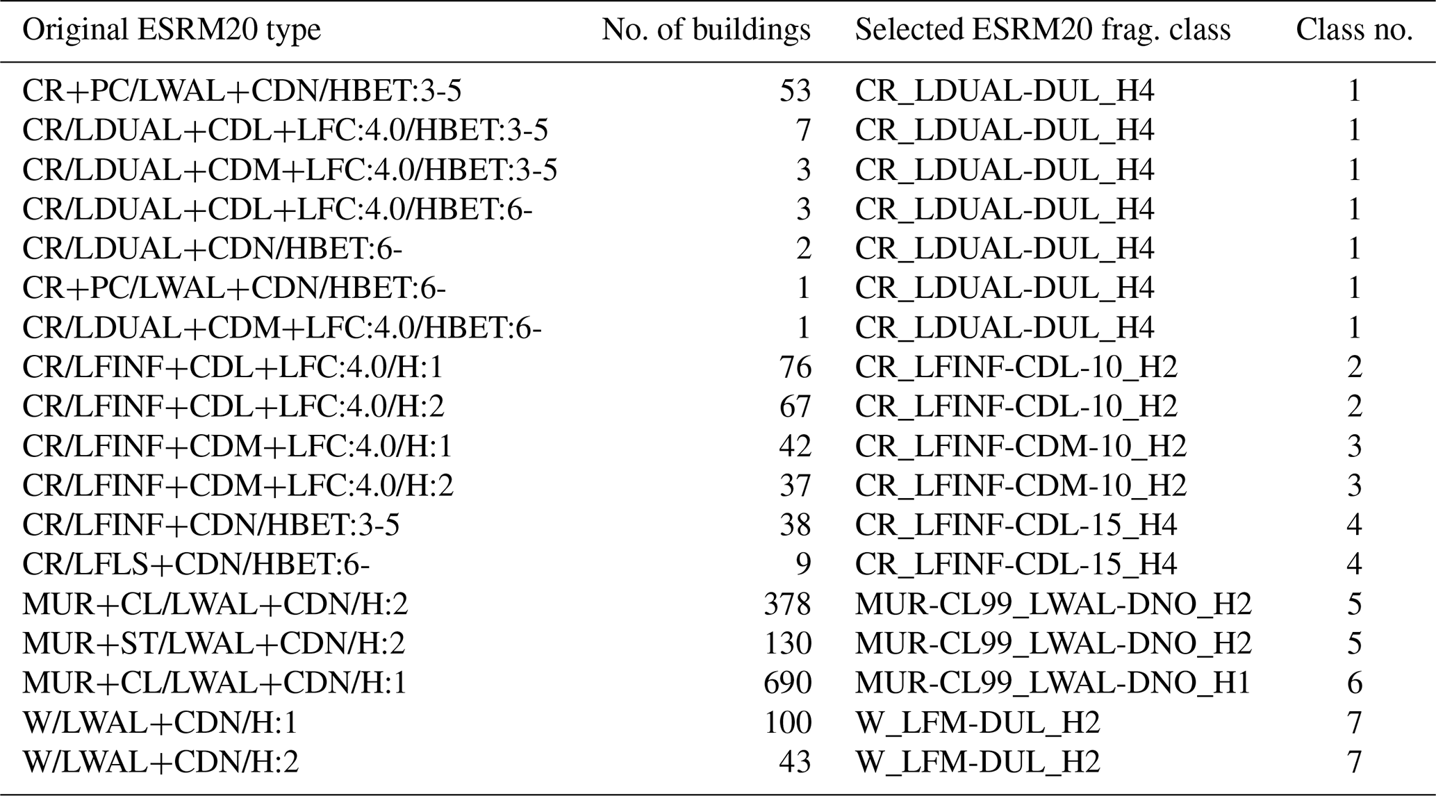
Table A2Summary of the exposure based on the European exposure model for the municipality of Le Teil.
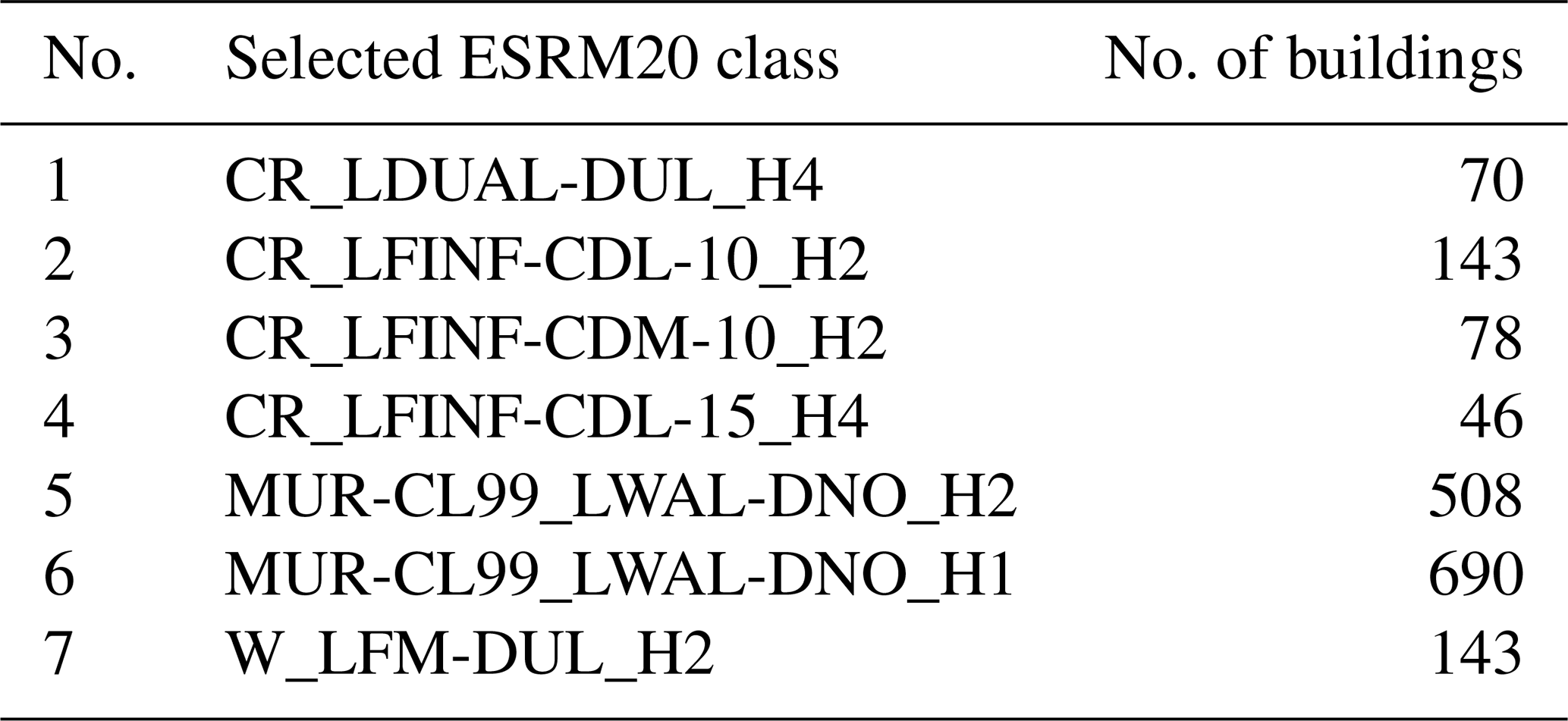
Table A3Summary of the BRGM exposure model for the municipality of Le Teil.
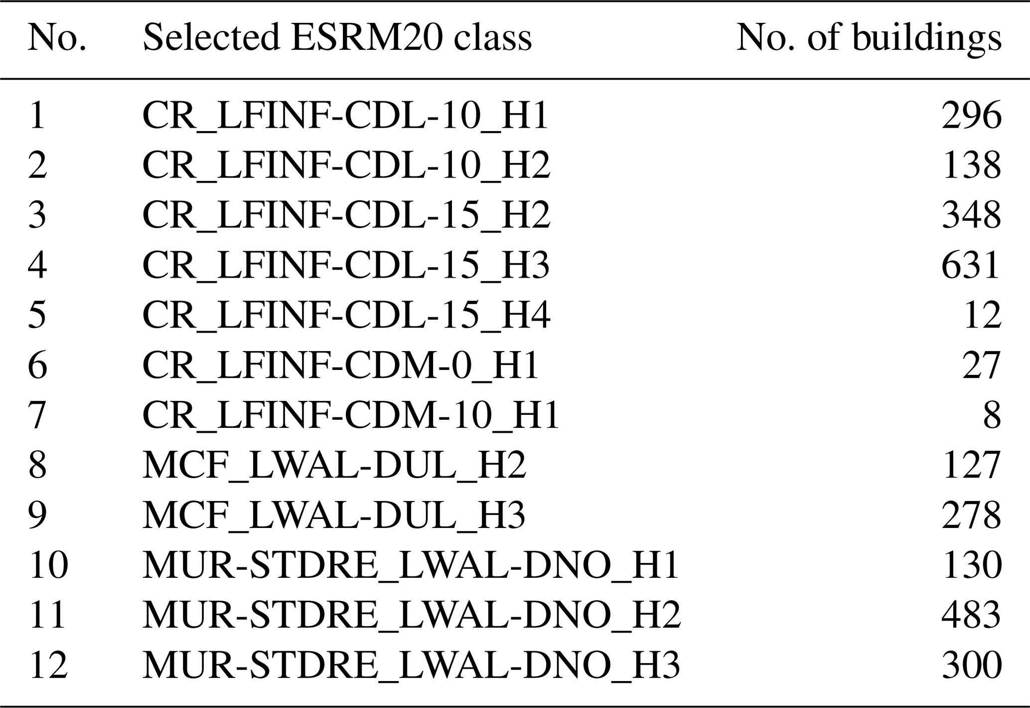
Table A4Conversion of the damage scale of the ESRM20 fragility models to the EMS-98 damage scale used for the comparisons.
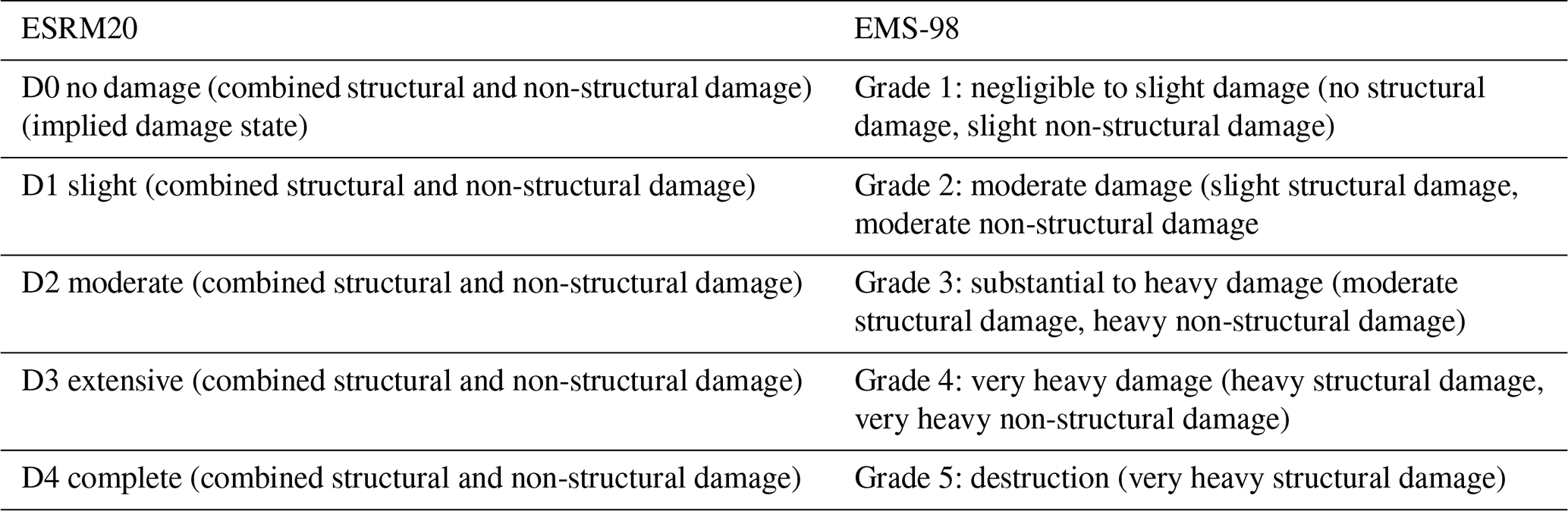
Table A5Empirical probabilities of the colour tags for the 174 entries that were excluded from the damage dataset used for the calculations.
Code and data are available upon request.
KT: conceptualization, data curation, formal analysis, investigation, methodology, software, validation, visualization, writing (original draft preparation, review and editing). PG: conceptualization, data curation, formal analysis, investigation, methodology, software, supervision, validation, writing (original draft preparation, review and editing). CN: conceptualization, data curation, funding acquisition, methodology, project administration, supervision, writing (original draft preparation, review and editing). HC, LD: writing (review and editing).
The contact author has declared that none of the authors has any competing interests.
Publisher's note: Copernicus Publications remains neutral with regard to jurisdictional claims made in the text, published maps, institutional affiliations, or any other geographical representation in this paper. While Copernicus Publications makes every effort to include appropriate place names, the final responsibility lies with the authors.
This article is part of the special issue “Harmonized seismic hazard and risk assessment for Europe”. It is not associated with a conference.
We would like to thank the French Association for Earthquake Engineering (AFPS) for providing access to the original earthquake damage dataset. Moreover, we are grateful to the editor and the referees for their very constructive comments.
This research has been supported by the Directorate-General for Risk Prevention (DGPR) of the French Ministry of Ecological Transition and Territorial Cohesion (Convention BRGM – DGPR 2023).
This paper was edited by Fabrice Cotton and reviewed by Cecilia I. Nievas and one anonymous referee.
Ake, J., Munson, C., Stamatakos, J., Juckett, M., Coppersmith, K., and Bommer, J.: Updated Implementation Guidelines for SSHAC Hazard Studies, United States Nuclear Regulatory Commission, Washington, D.C., United States, https://www.nrc.gov/reading-rm/doc-collections/ nuregs/staff/sr2213/index.html (last access: 9 July 2024), 2018.
Baker, J. W. and Jayaram, N.: Correlation of Spectral Acceleration Values from NGA Ground Motion Models, Earthq. Spectra, 24, 299–317, https://doi.org/10.1193/1.2857544, 2008.
Bommer, J. J., Strasser, F. O., Pagani, M., and Monelli, D.: Quality Assurance for Logic-Tree Implementation in Probabilistic Seismic-Hazard Analysis for Nuclear Applications: A Practical Example, Seismol. Res. Lett., 84, 938–945, https://doi.org/10.1785/0220130088, 2013.
Caprio, M., Tarigan, B., Worden, C. B., Wiemer, S., and Wald, D. J.: Ground Motion to Intensity Conversion Equations (GMICEs): A Global Relationship and Evaluation of Regional Dependency, B. Seismol. Soc. Am., 105, 1476–1490, https://doi.org/10.1785/0120140286, 2015.
Causse, M., Cornou, C., Maufroy, E., Grasso, J.-R., Baillet, L., and El Haber, E.: Exceptional ground motion during the shallow Mw 4.9 2019 Le Teil earthquake, France, Commun. Earth Environ., 2, 14, https://doi.org/10.1038/s43247-020-00089-0, 2021.
CEA/LDG: Séisme de magnitude ML 5,4 le 11/11/2019 près de Le Teil (Ardèche), French Alternative Energies and Atomic Energy Commission (CEA), https://www-dase.cea.fr/actu/dossiers_scientifiques/2019-11-11/index.html (last access: 11 January 2024), 2011.
Crowley, H., Despotaki, V., Rodrigues, D., Silva, V., Toma-Danila, D., Riga, E., Karatzetzou, A., and Fotopoulou, S.: SERA Deliverable D26.3 – Methods for Developing European Commercial and Industrial Exposure Models and Update on Residential Model, EUCENTRE, http://www.sera-eu.org/export/sites/sera/home/.galleries/Deliverables/SERA_D26.2_Residential_Exposure_Models.pdf (last access: 9 July 2024), 2019.
Crowley, H., Despotaki, V., Rodrigues, D., Silva, V., Toma-Danila, D., Riga, E., Karatzetzou, A., Fotopoulou, S., Zugic, Z., Sousa, L., Ozcebe, S., and Gamba, P.: Exposure model for European seismic risk assessment, Earthq. Spectra, 36, 252–273, https://doi.org/10.1177/8755293020919429, 2020.
Crowley, H., Dabbeek, J., Despotaki, V., Rodrigues, D., Martins, L., Silva, V., Romão, X., Pereira, N., Weatherill, G., and Danciu, L.: European Seismic Risk Model (ESRM20), EFEHR Technical Report 002, V1.0.1, 84 pp., https://doi.org/10.7414/EUC-EFEHR-TR002-ESRM20, 2021a.
Crowley, H., Despotaki, V., Rodrigues, D., Silva, V., Costa, C., Toma-Danila, D., Riga, E., Karatzetzou, A., Fotopoulou, S., Sousa, L., Ozcebe, S., Gamba, P., Dabbeek, J., Romão, X., Pereira, N., Castro, J. M., Daniell, J., Veliu, E., Bilgin, H., Adam, C., Deyanova, M., Ademović, N., Atalic, J., Bessason, B., Shendova, V., Tiganescu, A., Zugic, Z., Akkar, S., and Hancilar, U.: European Exposure Model Data Repository (v1.0), Zenodo [data set], https://doi.org/10.5281/ZENODO.4062044, 2021b.
Crowley, H., Despotaki, V., Silva, V., Dabbeek, J., Romão, X., Pereira, N., Castro, J. M., Daniell, J., Veliu, E., Bilgin, H., Adam, C., Deyanova, M., Ademović, N., Atalic, J., Riga, E., Karatzetzou, A., Bessason, B., Shendova, V., Tiganescu, A., Toma-Danila, D., Zugic, Z., Akkar, S., and Hancilar, U.: Model of seismic design lateral force levels for the existing reinforced concrete European building stock, B. Earthq. Eng., 19, 2839–2865, https://doi.org/10.1007/s10518-021-01083-3, 2021c.
Dabbeek, J., Crowley, H., Silva, V., Weatherill, G., Paul, N., and Nievas, C. I.: Impact of exposure spatial resolution on seismic loss estimates in regional portfolios, B. Earthq. Eng., 19, 5819–5841, https://doi.org/10.1007/s10518-021-01194-x, 2021.
Danciu, L., Nandan, S., Reyes, C., Basili, R., Weatherill, G., Beauval, C., Rovida, A., Vilanova, S., Sesetyan, K., Bard, P.-Y., Cotton, F., Wiemer, S., and Giardini, D.: The 2020 update of the European Seismic Hazard Model: Model Overview, EFEHR Technical Report 001, V1.0.0, https://doi.org/10.12686/A15, 2021.
DeBruine, L.: faux: Simulation for Factorial Designs R package version 1.2.1, Zenodo [code], https://doi.org/10.5281/zenodo.2669586, 2023.
Duverger, C., Mazet-Roux, G., Bollinger, L., Guilhem Trilla, A., Vallage, A., Hernandez, B., and Cansi, Y.: A decade of seismicity in metropolitan France (2010–2019): the CEA/LDG methodologies and observations, BSGF – Earth Sci. Bull., 192, 25, https://doi.org/10.1051/bsgf/2021014, 2021.
EMSC: M 4.9 – FRANCE – 2019-11-11 10:52:45 UTC, https://www.emsc-csem.org/Earthquake/earthquake.php?id=804595 (last access: 11 January 2024), 2019.
European Committee for Standardization: Eurocode 8: Design of structures for earthquake resistance – Part 1: General rules, seismic actions and rules for buildings, https://www.boutique.afnor.org/en-gb/standard/nf-en-19981/eurocode-8-design-of-structures-for-earthquake-resistance-part-1-general-ru/fa103832/25574 (last access: 9 July 2024), 2004.
Faenza, L. and Michelini, A.: Regression analysis of MCS intensity and ground motion parameters in Italy and its application in ShakeMap, Geophys. J. Int., 180, 1138–1152, https://doi.org/10.1111/j.1365-246X.2009.04467.x, 2010.
Gerstenberger, M. C., Marzocchi, W., Allen, T., Pagani, M., Adams, J., Danciu, L., Field, E. H., Fujiwara, H., Luco, N., Ma, K. -F., Meletti, C., and Petersen, M. D.: Probabilistic Seismic Hazard Analysis at Regional and National Scales: State of the Art and Future Challenges, Rev. Geophys., 58, e2019RG000653, https://doi.org/10.1029/2019RG000653, 2020.
GEM Foundation: KothaEtAl2020Site, openquake 3.18 reference, https://docs.openquake.org/oq-engine/3.17/reference/openquake.hazardlib.gsim.html?highlight=kothaetal2020site#openquake.hazardlib.gsim.kotha_2020.KothaEtAl2020Site (last access: 9 July 2024), 2023a.
GEM Foundation: KothaEtAl2020ESHM20SlopeGeology, openquake 3.18 reference, https://docs.openquake.org/oq-engine/3.17/reference/openquake.hazardlib.gsim.html?highlight=slopegeology#openquake.hazardlib.gsim.kotha_2020.KothaEtAl2020ESHM20SlopeGeology (last access: 9 July 2024), 2023b.
Goulet, J. A., Michel, C., and Kiureghian, A. D.: Data‐driven post‐earthquake rapid structural safety assessment, Earthq. Eng. Struct. D., 44, 549562, https://doi.org/10.1002/eqe.2541, 2015.
Grünthal, G.: European Macroseismic Scale 1998, Conseil de l'Europe, Luxembourg, https://media.gfz-potsdam.de/gfz/sec26/resources/documents/PDF/EMS-98_Original_englisch.pdf (last access: 9 July 2024), 1998.
Higham, N. J.: Computing the nearest correlation matrix – a problem from finance, IMA J. Numer. Anal., 22, 329–343, https://doi.org/10.1093/imanum/22.3.329, 2002.
Jayaram, N. and Baker, J. W.: Correlation model for spatially distributed ground-motion intensities, Earthq. Eng. Struct. D., 38, 1687–1708, https://doi.org/10.1002/eqe.922, 2009.
Kotha, S. R., Weatherill, G., Bindi, D., and Cotton, F.: A regionally-adaptable ground-motion model for shallow crustal earthquakes in Europe, B. Earthq. Eng., 18, 4091–4125, https://doi.org/10.1007/s10518-020-00869-1, 2020.
Lagomarsino, S. and Giovinazzi, S.: Macroseismic and mechanical models for the vulnerability and damage assessment of current buildings, B. Earthq. Eng., 4, 415–443, https://doi.org/10.1007/s10518-006-9024-z, 2006.
Mak, S. and Schorlemmer, D.: A Comparison between the Forecast by the United States National Seismic Hazard Maps with Recent Ground-Motion Records, B. Seismol. Soc. Am., 106, 1817–1831, https://doi.org/10.1785/0120150323, 2016.
Marzocchi, W., Taroni, M., and Selva, J.: Accounting for Epistemic Uncertainty in PSHA: Logic Tree and Ensemble Modeling, B. Seismol. Soc. Am., 105, 2151–2159, https://doi.org/10.1785/0120140131, 2015.
Matrix package authors and Oehlschlägel, J.: Matrix: Sparse and Dense Matrix Classes and Methods, https://cran.r-project.org/web/packages/Matrix/index.html (last access: 20 December 2023), 2023.
Monfort, C. and Roullé, A.: Estimation statistique de la répartition des classes de sol Eurocode 8 sur le territoire français – Phase 1: Rapport final, BRGM, https://infoterre.brgm.fr/rapports//RP-66250-FR.pdf (last access: 9 July 2024), 2016.
Musson, R. M. W., Grünthal, G., and Stucchi, M.: The comparison of macroseismic intensity scales, J. Seismol., 14, 413–428, https://doi.org/10.1007/s10950-009-9172-0, 2010.
Negulescu, C., Smai, F., Quique, R., Hohmann, A., Clain, U., Guidez, R., Tellez-Arenas, A., Quentin, A., and Grandjean, G.: VIGIRISKS platform, a web-tool for single and multi-hazard risk assessment, Nat. Hazards, 115, 593–618, https://doi.org/10.1007/s11069-022-05567-6, 2023.
OpenStreetMap contributors: OpenStreetMap, https://planet.osm.org (last access: 9 July 2024), https://www.openstreetmap.org (last access: 9 July 2024), 2017.
Pagani, M., Monelli, D., Weatherill, G., Danciu, L., Crowley, H., Silva, V., Henshaw, P., Butler, L., Nastasi, M., Panzeri, L., Simionato, M., and Vigano, D.: OpenQuake Engine: An Open Hazard (and Risk) Software for the Global Earthquake Model, Seismol. Res. Lett., 85, 692–702, https://doi.org/10.1785/0220130087, 2014.
Perez, R.: Risque sismique pour l'analyse des dommages observés suite au séisme du Teil, GCRN & BRGM, 2020.
R Core Team: R: A Language and Environment for Statistical Computing, https://www.r-project.org/ (last access: 20 December 2023), 2023.
Ritz, J.-F., Baize, S., Ferry, M., Larroque, C., Audin, L., Delouis, B., and Mathot, E.: Surface rupture and shallow fault reactivation during the 2019 Mw 4.9 Le Teil earthquake, France, Commun. Earth Environ., 1, 10,, https://doi.org/10.1038/s43247-020-0012-z, 2020.
Rood, A. H., Rood, D. H., Stirling, M. W., Madugo, C. M., Abrahamson, N. A., Wilcken, K. M., Gonzalez, T., Kottke, A., Whittaker, A. C., Page, W. D., and Stafford, P. J.: Earthquake Hazard Uncertainties Improved Using Precariously Balanced Rocks, AGU Adv., 1, e2020AV000182, https://doi.org/10.1029/2020AV000182, 2020.
Schlupp, A., Sira, C., Maufroy, E., Provost, L., Dretzen, R., Bertrand, E., Beck, E., and Schaming, M.: EMS98 intensities distribution of the “Le Teil” earthquake, France, 11 November 2019 (Mw 4.9) based on macroseismic surveys and field investigations, CR Geosci., 353, 465–492, https://doi.org/10.5802/crgeos.88, 2022.
Sedan, O., Negulescu, C., Terrier, M., Roulle, A., Winter, T., and Bertil, D.: Armagedom — A Tool for Seismic Risk Assessment Illustrated with Applications, J. Earthq. Eng., 17, 253–281, https://doi.org/10.1080/13632469.2012.726604, 2013.
Silva, V., Crowley, H., Pagani, M., Monelli, D., and Pinho, R.: Development of the OpenQuake engine, the Global Earthquake Model's open-source software for seismic risk assessment, Nat. Hazards, 72, 1409–1427, https://doi.org/10.1007/s11069-013-0618-x, 2014.
Silva, V., Brzev, S., Scawthorn, C., Yepes, C., Dabbeek, J., and Crowley, H.: A Building Classification System for Multi-hazard Risk Assessment, Int. J. Disast. Risk Sc., 13, 161–177, https://doi.org/10.1007/s13753-022-00400-x, 2022.
Taillefer, N., Arroucau, P., Leone, F., Defossez, S., and Clément, C.: Association Française du Génie Parasismique: rapport de la mission du séisme du Teil du 11 novembre 2019 (Ardèche), Association Française du Génie Parasismique, https://www.afps-seisme.org/file/1484 (last access: 9 July 2024), 2021.
USGS: M 4.8–5 km WNW of Rochemaure, France, https://earthquake.usgs.gov/earthquakes/eventpage/us60006a6i/moment-tensor (last access: 9 July 2024), 2019.
Wald, D. J., Worden, C. B., Thompson, E. M., and Hearne, M.: ShakeMap operations, policies, and procedures, Earthq. Spectra, 38, 756–777, https://doi.org/10.1177/87552930211030298, 2022.
Weatherill, G., Kotha, S. R., and Cotton, F.: A regionally-adaptable “scaled backbone” ground motion logic tree for shallow seismicity in Europe: application to the 2020 European seismic hazard model, B. Earthq. Eng., 18, 5087–5117, https://doi.org/10.1007/s10518-020-00899-9, 2020.
Wells, D. L. and Coppersmith, K. J.: New empirical relationships among magnitude, rupture length, rupture width, rupture area, and surface displacement, B. Seismol. Soc. Am., 84, https://doi.org/10.1785/BSSA0840040974, 1994.
- Abstract
- Introduction
- Seismological and damage data
- Modelling assumptions
- Comparisons of estimated intensities
- Comparisons of estimated damage
- Conclusion
- Appendix A
- Code and data availability
- Author contributions
- Competing interests
- Disclaimer
- Special issue statement
- Acknowledgements
- Financial support
- Review statement
- References