the Creative Commons Attribution 4.0 License.
the Creative Commons Attribution 4.0 License.
 | 18 Dec 2023
Return levels of extreme European windstorms, their dependency on the North Atlantic Oscillation, and potential future risks
Matthew D. K. Priestley
David B. Stephenson
Adam A. Scaife
Daniel Bannister
Christopher J. T. Allen
David Wilkie
Windstorms are the most damaging natural hazard across western Europe. Risk modellers are limited by the observational data record to only ∼ 60 years of comprehensive reanalysis data that are dominated by considerable inter-annual variability. This makes estimating return periods of rare events difficult and sensitive to the choice of the historical period used. This study proposes a novel statistical method for estimating wind gusts across Europe based on observed windstorm footprints. A good description of extreme wind speeds is obtained by assuming that gust speed peaks over threshold are distributed exponentially, i.e. a generalised Pareto distribution having a zero shape parameter. The threshold and tail scale parameter are estimated at each location and used to calculate estimates of the 10- and 200-year return levels. The North Atlantic Oscillation (NAO) is particularly important for modulating lower return levels and modulating the threshold, with a less detectable influence on rarer extremes and the tail scale parameter. The length of historical data required to have the lowest error in estimating return levels is quantified using both observed and simulated time series of the historical NAO. For reducing errors in estimating 200-year return levels of an independent 10-year period, a data catalogue of at least 20 years is required. For lower return levels the NAO has a stronger influence on estimated return levels, and so there is more variability in estimates. Using theoretical estimates of future NAO states, return levels are largely outside the historical uncertainty, indicating significant increases in risk potential from windstorms in the next 100 years. Our method presents a framework for assessing high-return-period events across a range of hazards without the additional complexities of a full catastrophe model.
- Article
(10019 KB) - Full-text XML
-
Supplement
(4535 KB) - BibTeX
- EndNote


Extratropical cyclones (ETCs) are the dominant weather system across Europe in the winter season, contributing most of the precipitation (Hawcroft et al., 2012) and strong winds (Ulbrich et al., 2001). ETCs are commonly associated with extreme wind speeds (also known as windstorms) that can impact infrastructure, agriculture, and transport and cause loss of life (e.g. Browning, 2004; Schwierz et al., 2010; Kendon and McCarthy, 2015). The strongest storms such as Lothar (26 December 1999) and Kyrill (18 January 2007) caused total insured losses exceeding EUR 5.5 billion (2022 equivalent; PERILS AG, 2022), with economic losses far exceeding this.
Although long-range predictability of European windstorms exists (e.g. Scaife et al., 2014; Befort et al., 2019; Degenhardt et al., 2023), extreme events are hard to predict and are simulated based on historical events and known natural variability. The main tools used to estimate rare events and their risk potential are catastrophe models (Grossi and Kunreuther, 2005). These models generally use reanalysis or climate model data as the driving hazard along with varying exposure and vulnerability data to quantify these rare risks. Catastrophe models must be able to quantify losses at long return periods, for example at the 200-year return level in order to comply with the Solvency II directive1. Complying with this solvency directive becomes more difficult as there are only a few decades of coherent observational data from the historical period. Therefore, it is paramount to be able to understand and accurately quantify the risk of an event that would be at (or exceed) the 200-year return level. These risk estimates are often not freely available as catastrophe models are often licensed products with undisclosed vulnerability curves and calibration methods. Furthermore, catastrophe model event sets are often derived from century-long reanalyses or ensembles of climate model data, both of which may require substantial calibration or feature spurious trends (e.g. Bloomfield et al., 2018). Therefore, there is a clear need for a simple, transparent method to quantify high return levels associated with European windstorms for the wider risk community.
Projected extremes are dependent on the underlying distribution, and it is therefore important to understand the total variability in extreme events in a historical period (Woo, 2019). Research on extreme precipitation has shown an increase in the intensity of potential extremes when considering a larger sample sizes (Thompson et al., 2017). This is particularly important for European windstorms due to the pronounced decadal variability in storm numbers (Donat et al., 2011b; Dawkins et al., 2016; Cusack, 2023) and losses (Klawa and Ulbrich, 2003). With a varying length of historical record this may result in particularly stormy periods, such as the early 1990s, having a stronger influence on projected risks. Shorter records that do not cover this period would likely underestimate the risk potential due to the absence of this key component of historical variability. Consequently, a key question that arises is how variable estimations of extreme gusts are with historical records of differing lengths.
A well-known driver of the frequency and strength of cyclones and windstorms in Europe is the North Atlantic Oscillation (NAO; Hurrell et al., 2003). The NAO drives these variations through modulations of the large-scale pressure gradient across the North Atlantic Ocean, with more positive NAO phases leading to more cyclones with higher intensities than neutral or negative phases (Pinto et al., 2009; Gómara et al., 2014; Dawkins et al., 2016). With a changing climate, it is expected that positive NAO states will become more common (Fabiano et al., 2021) and cyclone wind speeds will become stronger (Priestley and Catto, 2022). It should therefore be expected that the NAO would modulate extreme gusts across Europe in both a historical and future climate, although the extent of this has currently not been explored.
Consequently, the four main questions to be addressed in this study are as follows:
-
Can 200-year return level gust speeds from European windstorms be reliably estimated using openly available observed windstorm footprints?
-
How important is the NAO in modulating high-return-level gust speeds?
-
How does the length of the historical record and choice of period influence return level estimates?
-
How could expected changes in the NAO under climate change lead to changing return levels?
2.1 Footprint database
For analysing historical windstorms, a set of spatially coherent and validated footprints are required at high spatial resolution. Windstorm footprints are summaries of the overall hazard and are maps of maximum wind gust speed over a period of 72 h. The Windstorm Information Service (WISC; WISC, 2017) project provided a set of footprints based on historical events for analysing the range, severity, and impact of historical windstorms (e.g. Koks and Haer., 2020; Welker et al., 2021). Footprints were produced by the UK Met Office through the downscaling of ERA-Interim and ERA-20C reanalysis data. The ERA-20C footprints range from 1940–2010 and ERA-Interim footprints from 1979–2014. In this study, the ERA-20C footprints from 1950–1979 and the ERA-Interim footprints from 1980–2014 are used. There are some differences in footprints generated from the two reanalyses, although robust differences in footprint intensity cannot be determined. The footprints provide spatial estimates at 4.4 km resolution of the maximum 3 s wind gust at 10 m elevation over the 72 h period of each downscaled storm (WISC, 2017). The WISC footprints are similar to those provided by the XWS project (Roberts et al., 2014) but extend further back in time and are downscaled to a higher spatial resolution.
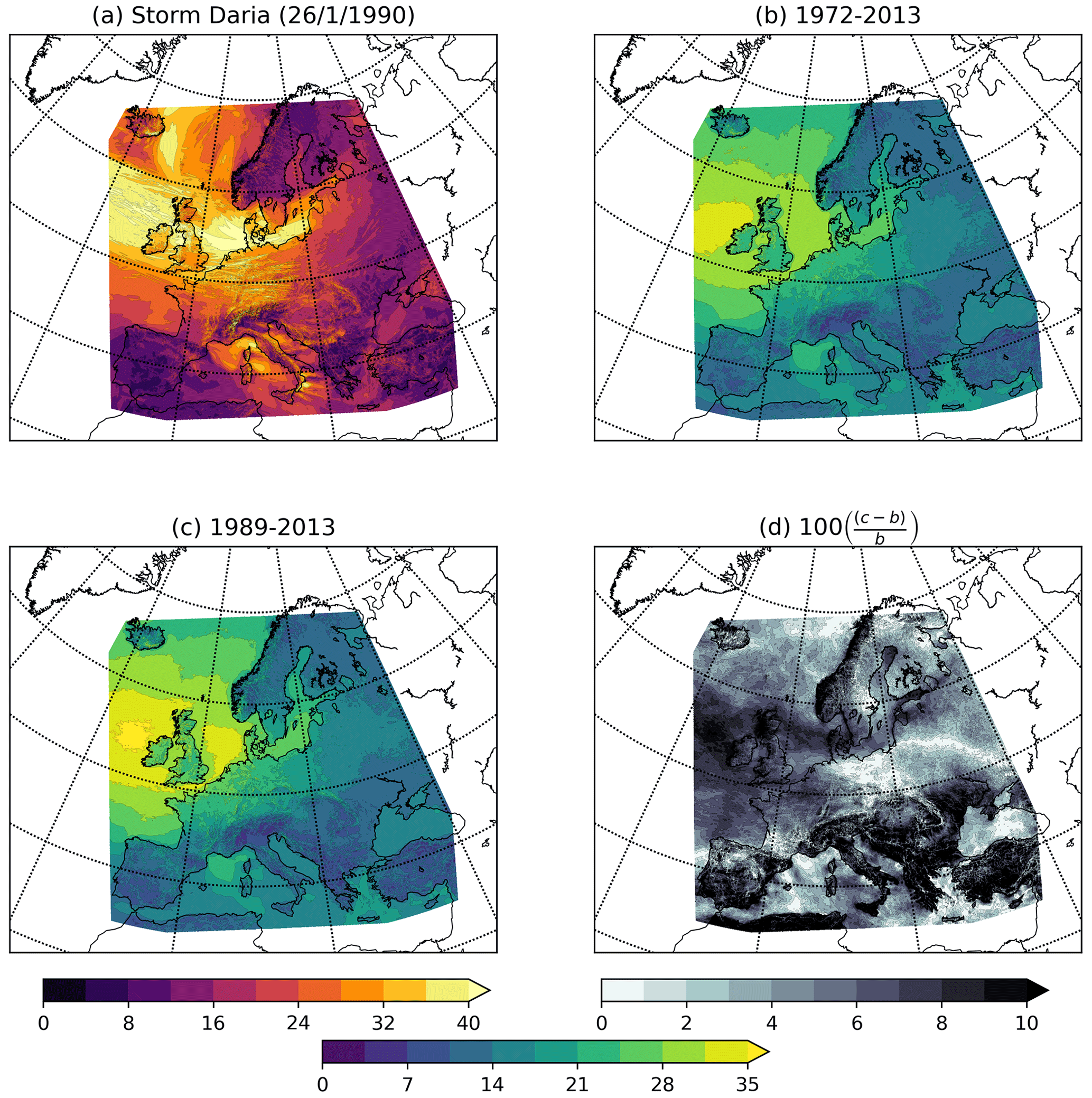
Figure 1Storm footprints from the WISC catalogue. (a) Footprint of Storm Daria on 26 January 1990. Average footprint of two different length time periods: (b) 1972–2013 and (c) 1989–2013. (d) The difference between the two periods as a percentage. Units are metres per second (m s−1).
The storms to be downscaled were selected from a set of objectively identified cyclone tracks (Hodges, 1994, 1995), with those chosen being of relevance to the insurance industry and also those exceeding a pre-determined intensity threshold (Steptoe, 2017). The time period of the cyclone track for downscaling is defined as ± 36 h of the maximum intensity of the storm, with the maximum intensity defined as the time of maximum 925 hPa wind speed over land. The downscaling is performed in two steps. Firstly the reanalysis data acts as boundary conditions for a 12 km version of the Met Office Unified Model that is initialised on 4 consecutive days for 30 h. Following this, the 12 km model acts as boundary conditions for the 4.4 km model. The 4 consecutive days of 4.4 km downscaled data is then concatenated and the relevant time period of the track extracted. The final footprint is then the maximum wind gust value at each grid point. A spatial Gaussian filter is applied to the footprint in order to eliminate spurious extremes generated in the downscaling. All the footprints have been validated against observations and result in 124 high-resolution windstorm footprints for the period 1950–2014 for use in this analysis.
2.2 NAO data
The NAO data used in this study are obtained from the NOAA CPC (https://www.cpc.ncep.noaa.gov/products/precip/CWlink/pna/nao.shtml, last access: 12 December 2023) and are calculated utilising rotated principal component analysis as described in Barnston and Livezey (1987). NAO indices are calculated using rotated principal component analysis applied to monthly 500 mb geopotential height fields from 1950–2000 that are then interpolated to daily values. NAO daily values are available for the period 1950–present and are standardised using the mean and standard deviation of the 1950–2000 climatological values. The NAO index for each storm is taken from the middle day of the 72 h WISC footprints.
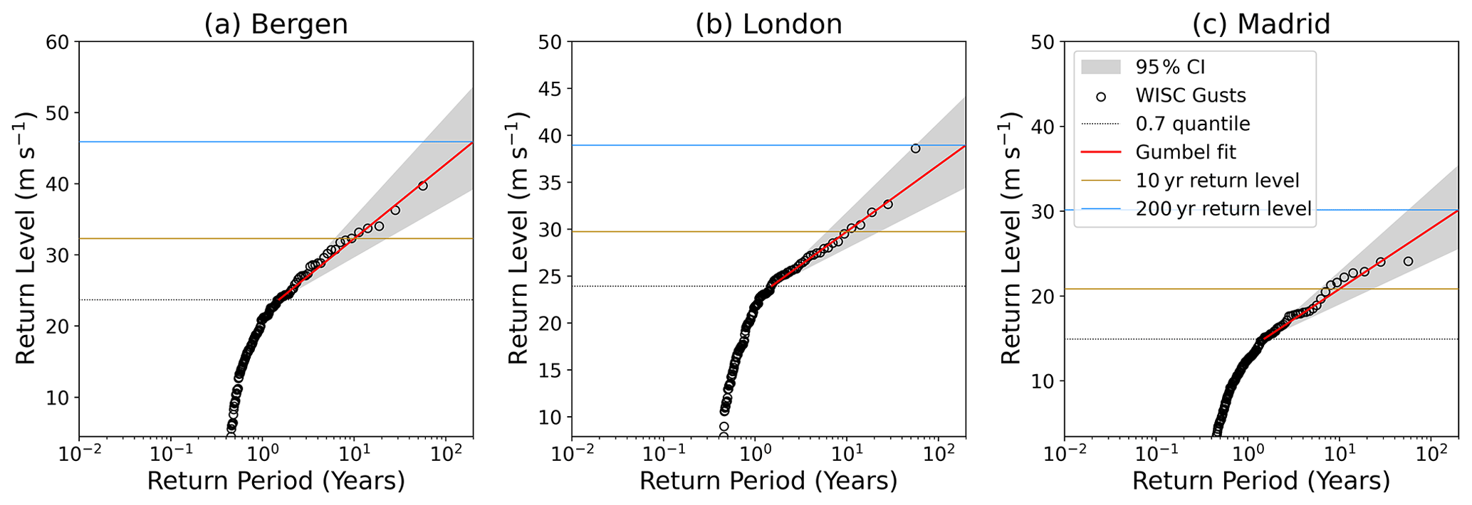
Figure 2Tests of the Gumbel fit for high return periods at the three representative locations: (a) Bergen (60.4∘ N, 5.1∘ E), (b) London (51.5∘ N, 0.4∘ W), and (c) Madrid (40.4∘ N, 3.8∘ W). The gusts for each location from 1950–2014 are plotted against their return period. The dotted black line indicates the 0.7 quantile, the red line indicates the Gumbel fit, the dark yellow line is the 10-year return period, and the blue line is the 200-year return period. The 95 % confidence intervals are estimated from a gamma distribution with shape and scale defined from the σ parameter and number of footprints and are shown by the grey shaded region.
2.3 Statistical methodology
For building the statistical model to estimate high-return-period windstorm gusts at any given location or grid point across Europe, the return period of gusts from the WISC footprints (e.g. storm Daria; Fig. 1a) first needs to be quantified. The return period is the expected time between successive events and therefore is equal to the reciprocal of the rate of the process. Therefore, the formulation of the return period (in years) of a wind speed (y) for an event Y>y is
where λ is the rate of storm occurrence (WISC footprints per year; ∼ 2.1). Windstorms can be separated into events with strong winds (S) and those without strong winds (). These events have different rates, λS and . For large return periods, it is assumed that the rate of occurrence for strong windstorms is considerably larger than for weak windstorms (). As the WISC data were constructed just for meteorologically intense and impactful windstorms, we define this as our strong storm subset, and therefore we know the rate of strong storms with strong gusts, thus following these assumptions .
The exceedance probability can then be factored as follows:
where u is a threshold that is large enough to use extreme value theory generalised Pareto fits to the model . By assuming that the tail shape parameter is zero and in the Gumbel domain of attraction, this gives exponentially distributed excesses above the threshold:
In Eq. (3), σ is the tail scale parameter that can be estimated by method of moments (Bowman and Shenton, 2006) from the mean excess above the threshold (u), yielding
Furthermore, the quantity can be estimated from the relative frequency of exceedances:
and so if u is taken to be the qth empirical quantile (u=yq), then . As the WISC data are already a sub-selection of extreme wind speeds, a relatively low quantile (q=0.7) is chosen to model the tail of the distribution. The sensitivity of the estimated return levels to the value of u are discussed below.
Equating from Eq. (1) with from Eqs. (2) and (3) gives a simple prediction for the T-year return level that is based on the qth empirical quantile (u), the mean excess above threshold (), and the rate of windstorm occurrence ():
In order to test the functionality of the method, the statistical model is applied to the WISC data at three example locations. These three locations vary in latitude and represent varying influence from the leading pattern of variability, the NAO. The three locations are Bergen (60.4∘ N, 5.1∘ E), London (51.5∘ N, 0.4∘ W), and Madrid (40.4∘ N, 3.8∘ W). Figure 2 shows a demonstration of the statistical model. The three locations have different gust speed distributions, with higher gusts at the northernmost locations. The estimation of the 10-year return level at each location is very similar from our model and from the empirical data. However, the 200-year return levels are larger than any gust from the WISC footprints at each location. For Bergen the 200-year estimate is 45.9 m s−1 (39.7 m s−1 WISC max), for London 39.0 m s−1 (38.6 m s−1), and for Madrid 30.1 m s−1 (24.1 m s−1). The statistical model has also been applied to the five largest cities across Europe (not shown) and to a set of windstorm footprints derived from the ERA5 re-analysis (Appendix A) and provided similar results. Our model is therefore able to estimate high-return-period gusts that are unprecedented in the observations.
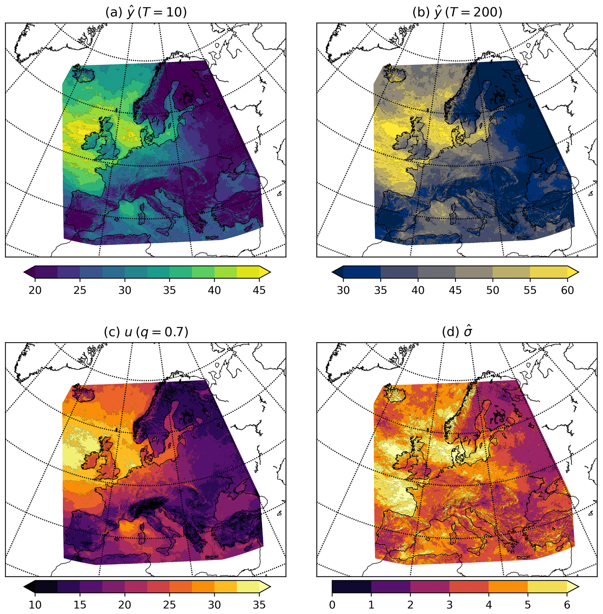
Figure 3Hazard maps generated by the statistical model for the (a) 10-year and (b) 200-year return levels across Europe. (c) The 0.7 quantile threshold used to calculate the return levels. (d) The mean excess (sigma) used in the return level calculations. All units are metres per second (m s−1).
The chosen empirical quantile is 0.7 for estimating the extreme gusts. Figure S1a–c in the Supplement demonstrates how the 200-year return level varies with a changing value of u (or q). When u is very small, there are large variations in (and large values of) the 200-year return level due to the inclusion of low gust speeds in our model fitting. There is a stabilisation in the 200-year return level for q≥ 0.7, with variations within 5 m s−1 for all three locations. This is the case up until the very highest thresholds, where larger variations in the 200-year return level are again noted; however, these high thresholds have a reduced number of footprints in the model fitting, so as with the low thresholds, these are unlikely to provide realistic estimates of the high return levels.
3.1 Wind gust hazard maps
By applying this method to all grid points of the WISC footprints, estimates of the 200-year return levels can be produced for all of Europe (Fig. 3). The 10-year return level is also examined as it is a return level that is easier to validate with historical claims data. The 10-year (Fig. 3a) and 200-year (Fig. 3b) return levels show a maximum in the return levels across northwestern Europe and the North Atlantic Ocean. This is expected as this is the region of strongest gust speeds in the WISC footprints (Fig. 1b and c). Return levels decrease radially from the UK, with lower values across Iberia, Italy, eastern Scandinavia, and eastern and southeastern Europe. These lower values are associated with a lower frequency and reduced intensity of windstorms in the historical catalogue due to a greater distance from the main North Atlantic storm track (Priestley et al., 2020). The largest 200-year return levels exceed 60 m s−1 to the northwest of Ireland. Over land, the largest 200-year return levels are 55–60 m s−1 across eastern Scotland, northeastern England, and Denmark, with values above 40 m s−1 for the majority of the rest of the British Isles, northern France, Benelux, and Germany (Fig. 3b).
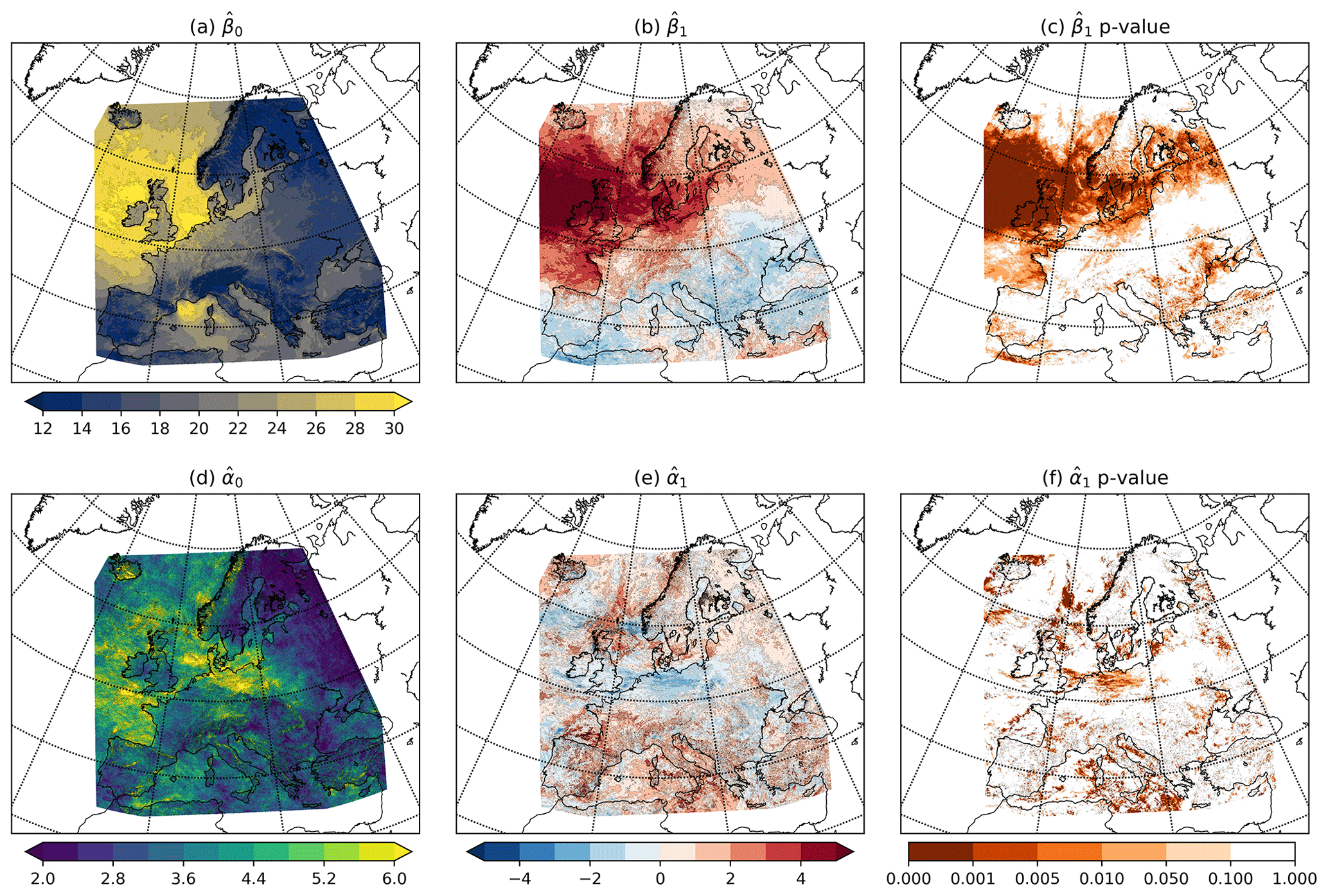
Figure 4Maps of the (a) , (b) , (d) , and (e) parameters for regressions applied to the WISC footprints from 1950–2014 with daily NAO covariate. Panels (c) and (f) show p values of the and regressions respectively. Units are (a, d) metres per second (m s−1) and (b, e) metres per second per SD ().
The dominant parameters in the return level estimates are the model threshold (u; Fig. 3c) and the mean excess above the threshold (; Fig. 3d). The spatial pattern of u (Fig. 3c) is similar to the return level maps (Fig. 3a and b) in that it features a maximum in the northwest of the domain in the area surrounding the North Atlantic. The magnitude of u decreases toward southern and eastern Europe. This pattern suggests a strong NAO influence, with larger values in the region where the NAO drives high wind speeds and damaging windstorms (Pinto et al., 2009). Unlike u, does not have the same north–south dipole over western Europe (Fig. 3d). Instead values vary much less, with only a 4–5 m s−1 variation across the entire WISC domain. The variation in is not coherent and is therefore consistent with this component being independent of large-scale patterns, such as the NAO.
3.2 Generalising the model to include an NAO covariate
The parameter u displays a pattern that is indicative of an NAO influence and can therefore be generalised to include such variations. If the threshold is chosen to be the qth empirical quantile, then and then and σ can be generalised to be a function of a covariate x. The covariate x will be the daily NAO index at the time of a WISC footprint occurrence. By estimating the threshold using linear quantile regression and estimating σ using generalised linear regression for a gamma distribution with identity link, this yields

Figure 5Dependence of gusts on the NAO at the three representative grid points: (a) Bergen (60.4∘ N, 5.1∘ E), (b) London (51.5∘ N, 0.4∘ W), and (c) Madrid (40.4∘ N, 3.8∘ W). Scatter points are the WISC grid point gusts against the daily NAO index. Horizontal dashed black line indicates the 0.7 quantile for each location. The red line is the q=0.7 estimation based on the NAO gust regression. The dark yellow line indicates the 10-year return level, and the blue line is the 200-year return level using the Gumbel domain estimation.
Applying these regressions to the WISC data yields the parameters shown in Fig. 4. The parameters (Fig. 4a and b) exhibit the typical NAO-influence pattern, with larger values and positive regression coefficients across the northwest of the WISC domain and smaller values and negative coefficients across eastern, southeastern, and southern Europe. This indicates that more northerly latitudes and northwestern European locations have a positive NAO–gust threshold relationship and vice versa. Furthermore, p values of this regression (Fig. 4c) indicate widespread significance of the NAO influence for northwestern and northern Europe, with large areas of p<0.001. The parameters (Fig. 4d and e) do not feature an NAO influence, and values are more variable across all of Europe. The north–south dipole is not evident, and it therefore appears that the NAO has minimal influence on the windstorm gust excesses. The significance testing (Fig. 4f) indicates there are isolated areas where the NAO influences σ, yet these are not widespread or indicative of a mode of variability. Despite this finding for the parameters, it may be that an NAO relationship across larger areas of Europe is undetectable in our small data sample and that with a larger pool of windstorm footprints a signal may emerge. Due to the undetectable signal in the parameters the NAO covariate is only applied to the threshold (u) in the statistical model, and therefore Eq. (6) becomes
Figure 5 shows the NAO covariate model (Eq. 9) tested at the same three grid points as previously. Each location features a different NAO relationship. The most northerly point, Bergen, has a strong positive relationship between return level and the NAO (p<0.01). An NAO of +1.5 standard deviations yields a 200-year return level of > 50 m s−1. For the London grid point, this NAO relationship is still positive, although weaker than for Bergen (p< 0.1), as would be expected. Finally, for the Madrid grid point an insignificant (p> 0.5) negative–neutral relationship is present, and therefore when the NAO is more positive, the estimated return level gets smaller. The reduced NAO sensitivity for the Madrid grid point is to be expected from the in-land and southerly nature of this location.
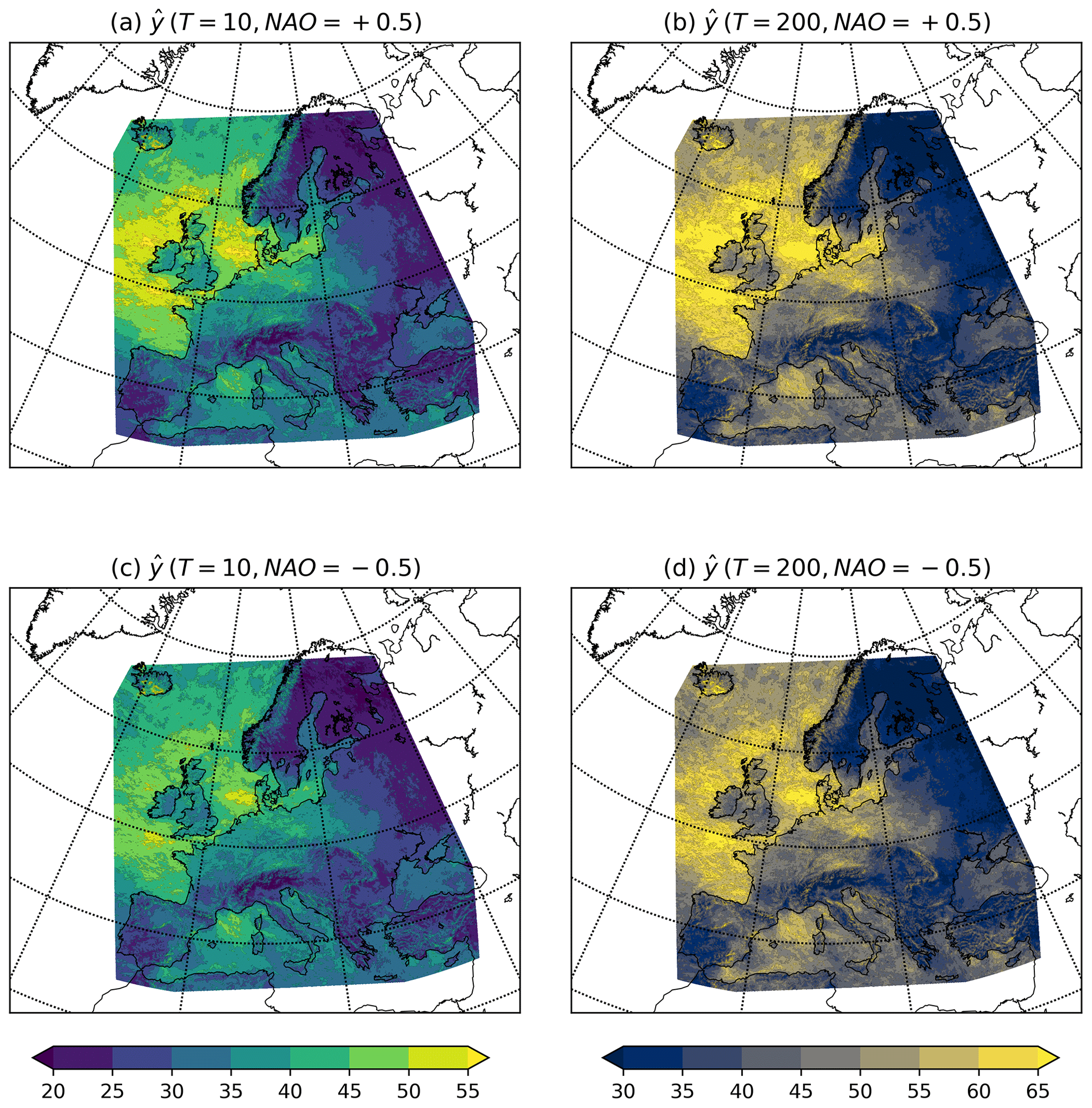
Figure 6NAO dependence of return levels. Maps of the (a, c) 10-year and (b, d) 200-year return level across Europe using the NAO covariate. Maps are shown for an NAO signal of (a, b) +0.5 and (c, d) −0.5. Units are metres per second (m s−1).
Applying the NAO covariate method to all grid points yields the return levels for the 10- and 200-year return periods shown in Fig. 6. The same regional variation and distribution in return levels across Europe are seen as in Fig. 3. Return levels are higher for the 200-year return period (Fig. 6b) than the 10-year (Fig. 6a) with values ∼ 10 m s−1 higher across northwestern Europe. It should be noted that the calculated 200-year return levels are higher when using the NAO covariate (Figs. 6b and 3b), with maximum values of > 65 m s−1 over the North Sea and North Atlantic Ocean and values exceeding 50 m s−1 across the northern British Isles, Denmark, and northern Germany. The variability in return level with an NAO state of +0.5 (Fig. 6a and b) and −0.5 (Fig. 6c and d) is also apparent for both return levels, with higher values of up to 5 m s−1 across the northwest of the domain for the NAO+ state (see also Fig. S2).
The spatial pattern of the 10- and 200-year return levels (Fig. 6) differs due to the differing contribution of u and the excesses () with return period (Fig. S3). The contribution of the NAO-dependent u decreases with increasing return period, and the contribution of the NAO-independent increases. Therefore, as the influence of the NAO is only detectable in the regression of u, it can be said that the relative importance of the NAO on our estimated return levels decreases with an increasing return period.
3.3 Sensitivity to choice of historical period
One factor that can contribute to the uncertainty in the estimation of the 200-year return level is the length of the historical catalogue. This is especially important for (re-)insurers and their need to understand risk in the next 10 years, as this is a time horizon for business planning, and 10 years is also the typical maximum service life of a catastrophe model. The varying length of catalogue has a substantial impact on the average footprint (Fig. 1b–d), and when applied to the statistical model at a return period of 200 years, these differences are likely to be amplified. Therefore, the understanding of future risk is likely to differ with these different length catalogues. The 200-year return level estimates vary considerably when using historical catalogues of different lengths (Fig. S4). The mean squared error (MSE) of the 200-year return level for historical catalogues from a year in the range of 1951–2014 relative to the full catalogue of 1950–2014 increases with shorter catalogue lengths (Fig. S4a) with grid point return level estimates being both under- or overestimated depending on the historical catalogue used (Fig. S4b and c).
In order to quantify how different catalogue lengths compare in their return level estimates, an independent time period is required for validation. For this, a 10-year time period of WISC footprints is taken (e.g. January 2005–December 2014), and the 200-year return levels are estimated. The historical catalogues for the preceding years starting at a length of 1 year and extending all the way out to 55 years (i.e. 2004, 2003–2004, 2002–2004, …, 1950–2004 in this example case) are taken and return levels estimated. The MSE of all catalogue return levels are then calculated relative to the 10-year validation period to quantify the optimal historical catalogue length required to minimise the error in estimated return levels. To account for natural variability all possible 10-year validation periods are tested with start years ranging from 1955 to 2005.
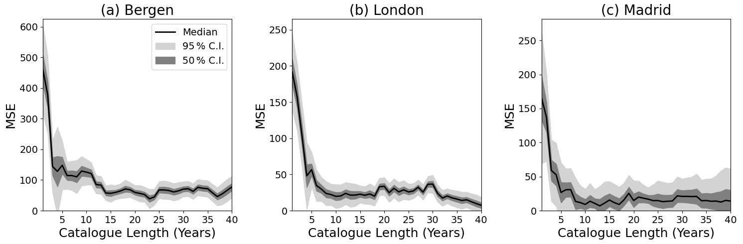
Figure 7Mean square error in the 200-year return level estimation of historical catalogues of different lengths against a subsequent 10-year period from the WISC catalogue for (a) Bergen, (b) London, and (c) Madrid. The solid black line shows the median mean squared error when using all possible periods. The dark and light grey areas represent the 50 % and 95 % confidence interval on the standard error respectively from the catalogues with different validation periods.
Applying this methodology to the same three grid points noted above we find that all locations (Fig. 7) feature a high MSE for the shortest catalogue lengths. The high MSE with short catalogue length is expected due to the limited sample of footprints contributing to the return level estimate. Increasing catalogue lengths to above 2 years causes a sharp reduction in the MSE at all locations, with limited improvements after ∼ 10–15 years. Therefore, historical catalogues longer than 10–15 years do not yield improvements in the return level MSE at these three locations. There are variations in the MSE estimate from year to year and large uncertainty in the MSE, which is an artefact of the limited data catalogue. With a limited historical catalogue, potential reductions in uncertainty or MSE for catalogue lengths longer than 40 years cannot be quantified. Greater uncertainty in MSE is also seen for the longest catalogue lengths at Madrid (Fig. 7c), which is a sampling artefact from having fewer long catalogue samples from the WISC data. Validation periods of different lengths (i.e. 5, 20 years) were also tested with conclusions being insensitive to this change (not shown).
3.4 Simulating the NAO for a more robust catalogue length estimation
For a more confident estimation of the optimal catalogue length and to assess the impact of data catalogues longer than 40 years in length, a time series of the NAO and the windstorm model parameters are simulated. The NAO is simulated as a sinusoidal variation of a period of 70 years (e.g. Wanner et al., 2001; Olsen et al., 2012; Wang et al., 2017) and amplitude of 1.5 standard deviations to match the variations from the WISC footprints (not shown). The WISC footprints occur at a rate of ∼ 2.1 per year, and the model is built to fit the top 30 % of these events; therefore, occurrences of extreme storms and their NAO phase can be estimated from these frequencies. This entire simulation is done for 1000 years (Fig. 8a).
Using the regressional relationships between the WISC footprints and the NAO state (Fig. 4a and b), the value of u (Fig. 8a) and σ can be estimated in the simulated time series and the resultant gust determined (Fig. 8b). Comparing the WISC grid point gusts for Bergen with our simulation (Figs. 5a and 8c), it is notable that the simulated gusts exceed those in the WISC dataset considerably, with gusts in excess of 60 m s−1. This is due to the longer time series in our simulation compared to the WISC dataset.
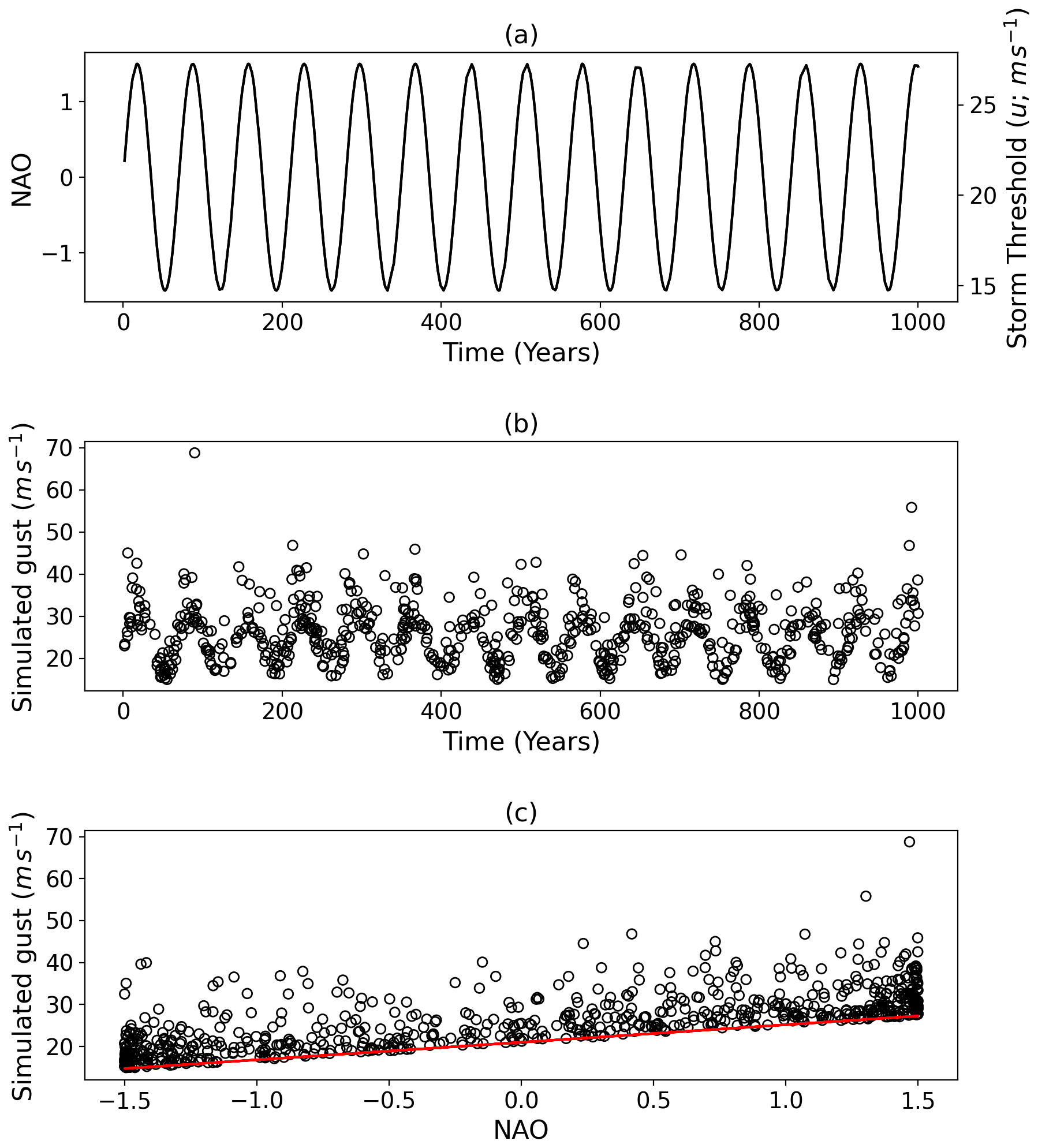
Figure 8Summary of simulated events at Bergen based on 1000-year NAO time series. (a) NAO phase and simulated storm threshold (u) at time of simulated events. (b) Simulated event gusts (m s−1). (c) NAO phase plotted against the simulated gusts. The solid red line shows the q=0.7 regression line.
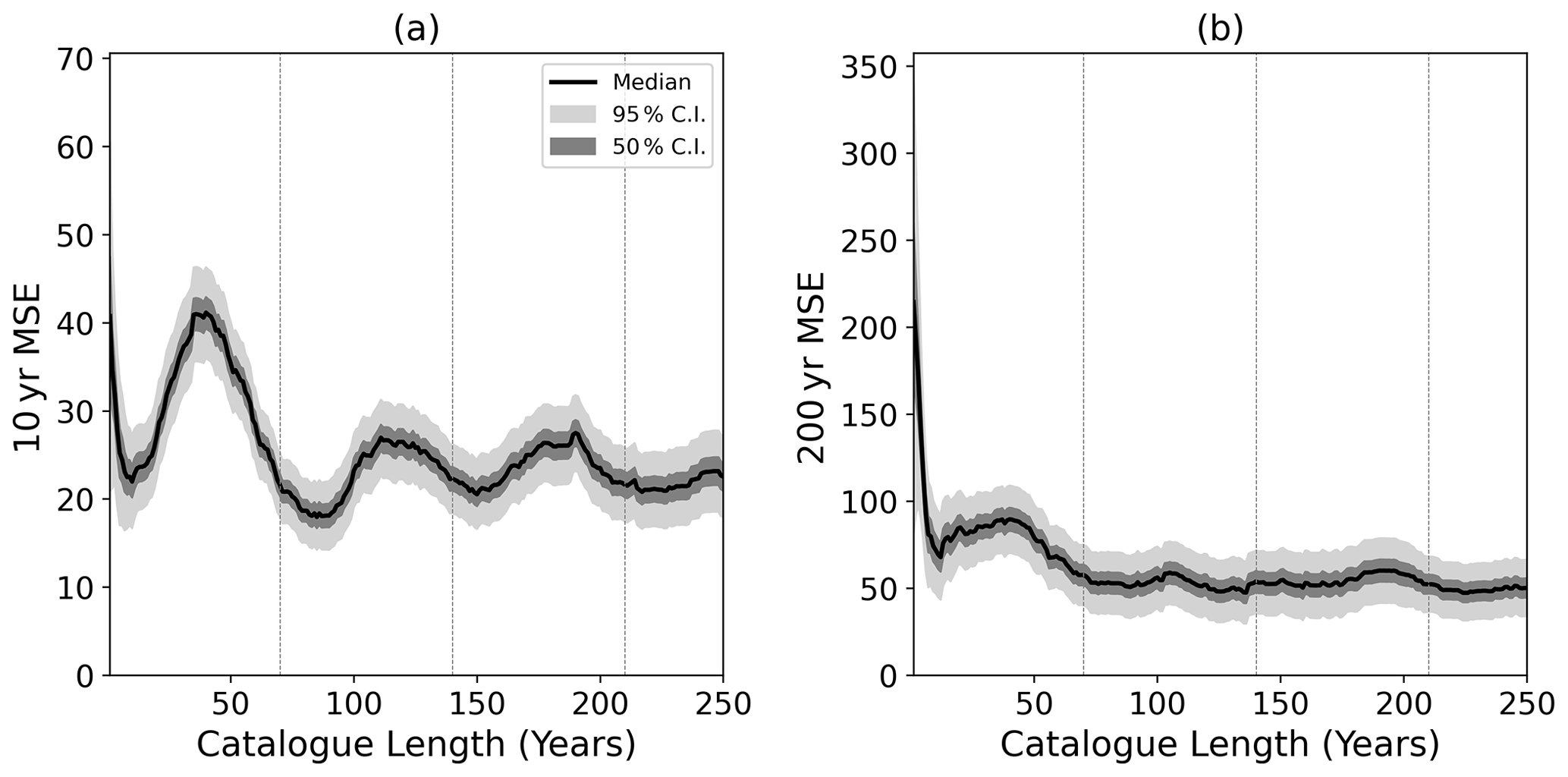
Figure 9Mean square error in the (a) 10-year and (b) 200-year return level estimation of historical catalogues of different lengths against a subsequent 10-year period with events from a 1000-year simulation for Bergen. The solid black line shows the median MSE from all possible periods. The dark and light grey areas represent the 50 % and 95 % confidence interval on the standard error respectively from the catalogues with different validation periods. Vertical dashed grey lines indicate the periodicity of the NAO used in simulations.
Using this simulated time series, the 10- and 200-year return levels can be estimated for different catalogue lengths for our three locations, with analysis performed as in Fig. 7. At Bergen the highest MSE is seen for the shortest catalogue lengths (Fig. 9). As in Fig. 7a, this is a result of the large inter-annual variability and the chance that 1 year will be representative of the following 10 being very small. For the 200-year return levels (Fig. 9b), a large reduction in the MSE is then seen as catalogue length increases to 15 years. For catalogue lengths of 15–50 years there are minimal changes in the MSE. Following this there is a slight reduction in MSE associated with capturing the full cycle of the imposed NAO cycle; however, there is overlap in the confidence intervals at 20 years and 70 years. Beyond 70 years and unlike the WISC results, there is now little variation in the MSE out to catalogue lengths in excess of 250 years and a much reduced spread and variation in the median. Therefore, there is limited benefit to using historical catalogues longer than ∼ 20 years when estimating the 200-year return level; however, if possible, a catalogue spanning a full NAO cycle is preferable. It should be noted that in Fig. 9 the MSE never reaches zero, indicating that a perfect return level estimate is never achieved. This is a result of unresolved natural variability that cannot be captured regardless of catalogue length.
At the 10-year return level (Fig. 9a) a reduction in MSE occurs up to a catalogue length of ∼ 10 years. Unlike the 200-year MSE, there is an oscillation in the MSE that has a period of ∼ 70 years and results in a maximum MSE for catalogue lengths of 40 years and a minimum after ∼ 80 years. The ∼ 70-year oscillation is consistent with the defined periodicity of the NAO simulation. The oscillation is present as the NAO influence is more pronounced for shorter return periods (Fig. S3). Consequently, the 10-year return levels more strongly reflect the variation in NAO, whereas the 200-year return levels will not. To reduce the MSE, the NAO signal of the historical catalogue relative to the 10-year validation period is important. For shorter catalogue lengths the NAO signal (and simulated gusts) will be similar; however, catalogue lengths of ∼ 35 years feature an NAO signal that is most different from the 10-year validation period and hence the MSE will be most different. When a full NAO cycle is sampled (∼ 70 years), the full proportion of NAO variability is captured and there is a minimum in MSE. For catalogue lengths longer than the prescribed NAO periodicity, the average NAO signal varies less and a dampening of the MSE variation is seen.
The structure of MSE evolution seen at Bergen (Fig. 9) is similar at London (Fig. S5) and Madrid (Fig. S6). For the 10-year return levels the oscillatory evolution at Bergen (Fig. 9a) is less apparent due to the weaker influence of the NAO on return levels (Figs. 4 and 5). As a result it is less important to sample a full cycle of the NAO, and the MSE varies little for catalogue lengths longer than ∼ 20 years.
3.5 Change in return levels from theoretical future NAO states
Recent estimates of the historical trend of the NAO have been upwards at a rate of +0.15 standard deviations per decade (1950–2020; Blackport and Fyfe, 2022). If it is assumed that the historically averaged NAO state is neutral, then a theoretical state of +1.5 standard deviations in 100 years is a plausible upper estimate. For estimating return levels of gusts in this theoretical future NAO state, events are simulated. The role of natural variability on return levels is also considered, and to account for this a 70-year period is used that features two 35-year periods at standard deviations compared to the reference state. For the historical state the reference is NAO neutral, and events are simulated at −0.5 and +0.5. For the future state the reference NAO is +1.5, and events are simulated at +1 and +2. The 70-year periods are simulated 100 000 times for our three grid points to obtain robust return levels. Selecting a model threshold and estimating the return levels of this two-component, variable NAO state model differs slightly from the earlier methodology and is documented in Appendix B.
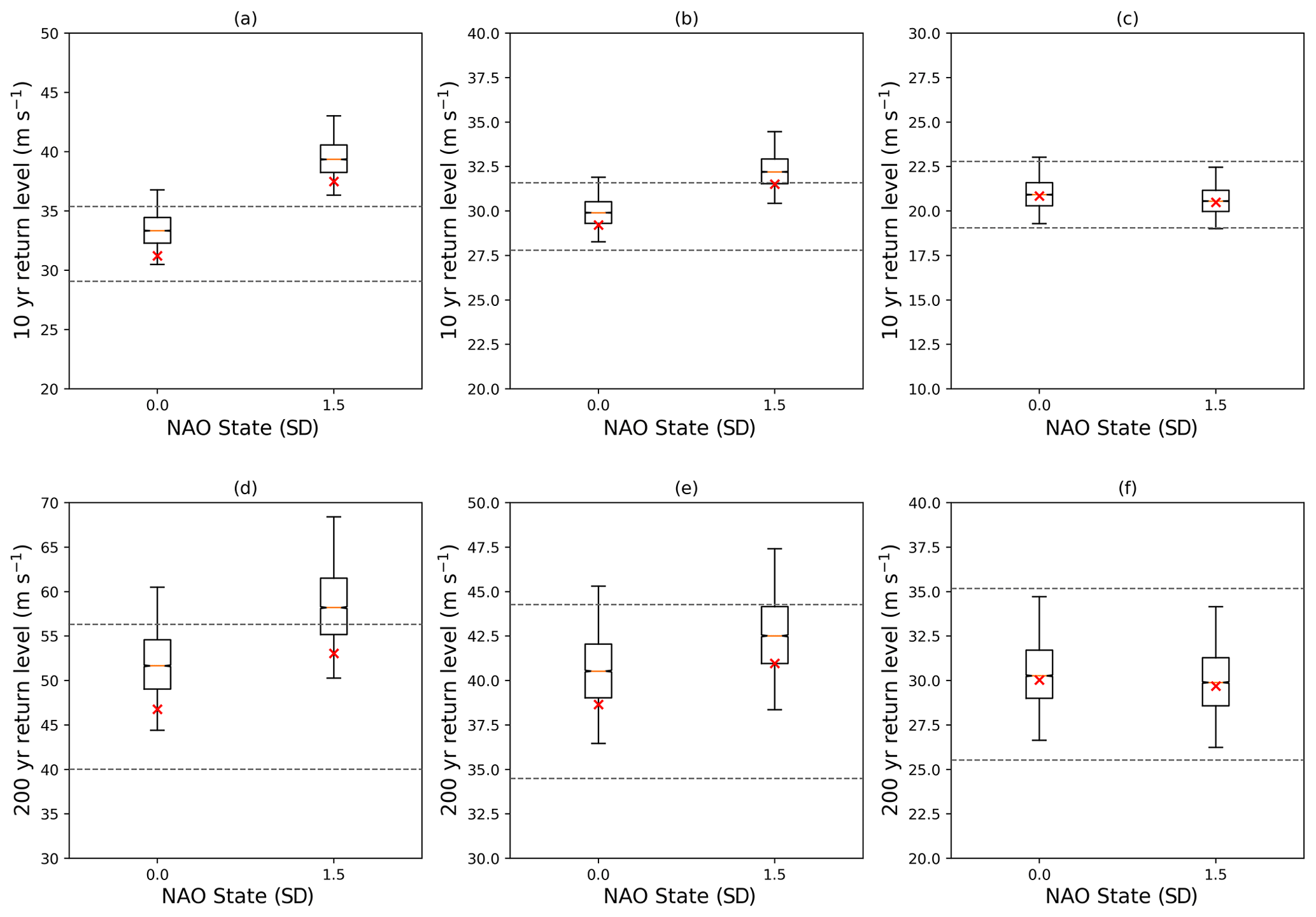
Figure 10Boxplots of estimated (a–c) 10-year and (d–f) 200-year return levels for (a, d) Bergen, (b, e) London, and (c, f) Madrid from simulated gusts. Return levels are estimated from 100 000 70-year simulations with NAO phase that varies to ± 0.5σ of a set NAO state. Boxplots show the median return level of these 100 000 simulations, and boxes extend to the 25th and 75th percentiles, with whiskers extending to the 2.5th and 97.5th percentiles. Red crosses signify the theoretical return level from a two-state NAO. Dashed horizontal grey lines indicate the 95 % confidence interval of the WISC 10- and 200-year return levels.
Using simulated gusts from our variable state model, the estimated return levels at Bergen for the NAO state of +1.5 are largely outside the WISC uncertainty for the 200-year return level (Fig. 10d). Therefore, if historical trends were to continue for the next 100 years, then the 200-year return levels would likely be unprecedented in this theoretical state. This is more evident at the 10-year return level (Fig. 10a) due to the increased influence of the NAO on these shorter return periods. For all NAO states the return levels estimated using the simulated, variable events are positively biased relative to theoretical values using exact parameters (Fig. 10). This is a result of the additional natural variability present in the simulated events from the varying NAO state (see Appendix B). Therefore, models that assume a stationary historical climate are also likely to be positively biased relative to actual return levels.
Similar changes in return levels are also seen for the future NAO state at London (Fig. 10b and e). However, as the NAO has a reduced influence the increase in 200-year return levels is less apparent with most estimates within the historical uncertainty (Fig. 10e). Nevertheless, the potential increases in 10-year return levels are still large enough to be greater than the historical uncertainty (Fig. 10b). At Madrid (Fig. 10c and f), the NAO influence is so small that any changes in the return levels are insignificant compared to the historical uncertainty.
This study has presented a method for estimating high-return-period gusts for the European domain based upon a set of observed windstorm footprints. This simple and transparent method is agnostic to the input dataset and operates without requiring calibration or the complexities of a full catastrophe model. However, it does not replace catastrophe models as no loss estimation or vulnerability module is included. The amount of historical data required to minimise errors in the return level estimation has been tested, and the sensitivity of return levels to theoretical future NAO states has been quantified. We raised several questions in Sect. 1, and the key conclusions that answer these are as follows:
-
Return levels at the 200-year return period have been quantified and associated uncertainties quantified. Return levels are higher over northwestern Europe, with the NAO playing a role in increasing (decreasing) return levels across northern (southern) Europe.
-
The NAO is important for setting the threshold for gust speed return levels, with the excess above the threshold being stochastically generated. The NAO modulates the lower return levels and is key in determining the threshold, with particular significance over northwestern Europe. The tail scale parameter is much more variable with a less detectable influence from the NAO.
-
Only 20 years of historical data is required to reduce errors in 200-year return level estimates made from the independent and subsequent 10-year period. Increasing historical records longer than this do not lead to meaningful improvements in return level estimates due to unresolved natural/inter-annual variability. Estimates of 10-year return levels are more sensitive to the length of historical catalogue due to the larger NAO influence.
-
Under theoretical future NAO states the 10- and 200-year return levels are likely to be unprecedented relative to historical values. Return level estimates are outside the historical uncertainty across northern Europe, with minimal changes across southern Europe. This would lead to considerably higher gusts and impacts than those currently considered.
Our modelling approach makes several simplifying assumptions. Firstly, for estimating the tail a zero shape parameter is used. This implies that an infinite return level is possible for the longest return periods. This is inaccurate, and in reality the shape parameter would be negative as there are frictional processes, instabilities, and limits to the amount of transferrable kinetic energy from a windstorm. However, we are confident in our estimations as the generated return curves are a good fit for the input data for numerous locations across Europe. These results provide additional data points to complement estimations made from more complex catastrophe models that will help guide risk modellers and aid understanding of potential European windstorm risks.
With regards to the data used, there is a historical limit due to the constraints of observations of severe European storms. This limit to 1950 may result in considerably large events that would constrain the model being missed or key components of the natural variability being excluded. However, with ongoing efforts to accurately represent historical storms (Hawkins et al., 2022), this may be improved in the future. Alongside this, the data used from the WISC project are only a small sample of all windstorms over Europe representing just the most intense events, and this may lead to a skewing of our return level estimations toward the worst case scenario.
Our methodology allows for the assessment of theoretical future return levels without the need of climate change simulations. However, these theoretical return level estimations only represent the changes in the circulation aspects of the NAO. One factor not considered in the large increase in return level for northern latitudes of Europe is the thermodynamic contribution. As a large amount of the potential increase in cyclone wind speeds across Europe is a result of moist processes (Dolores-Tesillos et al., 2022; Binder et al., 2023), it is likely that gusts would increase further beyond those predicted in the model here. These changes could have further implications on potential impacts. Only the NAO was considered a low-frequency modulator of windstorm intensity in our model. However, other phenomena have been shown to influence European winter weather through connections to the NAO. These are phenomena such as tropical precipitation (Scaife et al., 2017, 2019), the Atlantic multi-decadal oscillation (Börgel et al., 2020), and the El Niño–Southern Oscillation (Zhang et al., 2019a, b) to name a few. These low-frequency phenomena all have partial connection to the NAO and therefore may play a role in modulating windstorm strength through either the threshold or excesses in this model. Investigating potential linkages further may lead to improvements in the model and therefore more accurate return level estimations.
There are numerous future applications of our model. Firstly, this model could be used to investigate future changes in return levels. With projected future changes in the NAO and other leading modes of European weather variability (Fabiano et al., 2021; Blackport and Fyfe, 2022), the simulation of the NAO can be modified to apply trends and changes in variability to determine how this would affect the higher-return-period gusts. This could provide vital insight to the projected end-of-century increase in European storminess (Donat et al., 2011a; Zappa et al., 2013; Priestley and Catto, 2022; Dolores-Tesillos et al., 2022). Furthermore, seasonal forecasts of the NAO could be imposed to inform decision makers at shorter timescales. Consideration should be taken, however, due to the unresolved natural variability that is present in return level estimates regardless of the length of historical record. Finally, despite this model being developed for European windstorm risks, it could be easily adapted for other hazards/risks and act as a framework for assessing extreme events of other perils. Validation and testing would be required to meet regulatory and business requirements, but this model can act as an open-source and transparent method for investigating and quantifying a range of natural hazards.
In testing the applicability of the statistical model it has also been applied to a set of footprints from the ERA5 reanalysis (Hersbach et al., 2020). Footprints were created from a set of extratropical cyclone tracks. Tracks were identified following the method of Hodges (1994, 1995), which uses 850 hPa relative vorticity as a tracking variable. Tracks were created from 1-hourly data for the entire calendar year (1 January–31 December) for the period of 1980–2020. Full details of the cyclone identification and tracking method can be found in Hoskins and Hodges (2002). Tracks were filtered to those passing through a defined North Atlantic–European domain (30–75∘ N, 40∘ W–40∘ E) to encapsulate all tracks that would pass through continental Europe and to cover all the WISC domain.
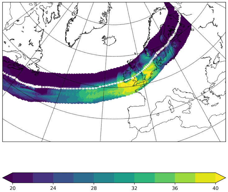
Figure A1Wind gust footprint from ERA5 of track forming on 20 January 1990 and dissipating on 28 January 1990. Coloured shading represents the maximum grid point wind gust in metres per second (m s−1). White line and crosses indicates the track and hourly track points respectively.
Footprints were created using hourly near-surface (10 m) wind gusts. These data provide the maximum 3 s wind gust at each grid point in the previous hour. At each track time step the gusts in the surrounding 5∘ are associated with the storm, and the maximum gust at each grid point across the lifecycle of the track is retained in order to create a coherent footprint. This method closely follows that of Roberts et al. (2014). An example footprint is shown in Fig. A1.
These footprints are then applied to the statistical model described in Sect. 2.3, and the analysis is performed as in Fig. 2. As there are many more footprints in our ERA5 dataset than from WISC, there are a considerably greater number of points to fit our model (Fig. A2a–c). As a result of the increase in the number of footprints, which are mainly of lower gust speeds, a higher threshold quantile for ERA5 is used than for the WISC footprints, with q=0.9 for the ERA5 footprints. Despite the increase in the number of footprints, the higher value of q, and the coarser resolution of the ERA5 data, the model fit is a good approximation for the data, and estimates of the 200-year return levels are able to be made.
The estimated 200-year return levels (Fig. A2a–c) are different from those estimated from WISC (Fig. 2a–c), as would be expected due to the differing input data. However, the values are consistent with those from WISC, with the main difference being an increase in the value of the 200-year return level for the London grid point (Fig. A2b). What is further re-assuring about the applicability of our model is the stability of the 10- and 200-year return levels for high quantiles used in the model (Fig. A2d–f). Estimations of these two return levels vary by less than 5 m s−1 for q≥0.9.
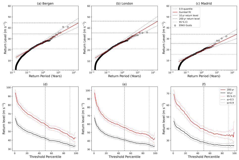
Figure A2(a–c) As Fig. 2 but using ERA5 footprints as an input. (d–f) The sensitivity of the 10-year (solid black) and 200-year (solid red) return levels to the choice of quantile threshold for (d) Bergen, (e) London, and (f) Madrid. Vertical black lines indicate the 0.5 and 0.9 quantiles. Thin red and black lines represent the 95 % confidence interval based upon the estimate of the σ parameter.
To gain insight into the effect of natural variations in modulators of the extremes, it is useful to consider a simple two-component mixture model. Consider a hazard process that is an equal mixture of two processes Ya(t) and Yb(t) that have exponential exceedances above thresholds a and b>a respectively. Then for y≥b,
If thresholds a and b are chosen to be the qth quantiles of Ya and Yb, then
Hence, the T-year return level is given by
which equals that derived in Eq. (7) if one sets . By integration of the probability density function, it is straightforward to derive the mean excess of this process above threshold :
which can be seen to be greater than or equal to σ. Hence, estimating σ by assuming it is equal to the mean excess will lead to a positive bias that vanishes only as u→b. In summary, the effect of natural variability in the tail location parameter is to cause the mean excess to overestimate the tail scale parameter, which in turn will lead to overestimates of return values for longer return periods. Put simply, if natural variability is not taken into account, the magnitudes of the extreme events will appear to be more variable than they actually are.
Model code is available from the author upon request.
ERA5 reanalysis is available from the Copernicus Climate Change Service Climate Data Store (https://doi.org/10.24381/cds.bd0915c6, Hersbach et al., 2018). WISC footprints and all associated documentation are available from the author upon request.
The supplement related to this article is available online at: https://doi.org/10.5194/nhess-23-3845-2023-supplement.
MDKP wrote the manuscript and performed all analysis. MDKP, DBS, and AAS devised the study and edited the manuscript. DBS formulated the statistical methodology. DB, CJTA, and DW provided feedback and comments on the manuscript.
The contact author has declared that none of the authors has any competing interests.
Publisher's note: Copernicus Publications remains neutral with regard to jurisdictional claims made in the text, published maps, institutional affiliations, or any other geographical representation in this paper. While Copernicus Publications makes every effort to include appropriate place names, the final responsibility lies with the authors.
This research was funded and supported by the WTW Research Network. Adam A. Scaife was also supported by the Met Office Hadley Centre Climate Programme funded by BEIS (Department for Business, Energy and Industrial Strategy) and Defra (Department for Environment, Food and Rural Affairs). We are grateful to the two anonymous reviewers whose comments have improved the quality of the manuscript.
This research was funded and supported by the WTW Research Network. Adam A. Scaife was also supported by the Met Office Hadley Centre Climate Programme funded by BEIS (Department for Business, Energy and Industrial Strategy) and Defra (Department for Environment, Food and Rural Affairs).
This paper was edited by Piero Lionello and reviewed by two anonymous referees.
Barnston, A. G. and Livezey, R. E.: Classification, Seasonality and Persistence of Low-Frequency Atmospheric Circulation Patterns, Mon. Weather Rev., 115, 1083–1126, https://doi.org/10.1175/1520-0493(1987)115<1083:CSAPOL>2.0.CO;2, 1987. a
Befort, D. J., Wild, S., Knight, J. R., Lockwood, J. F., Thornton, H. E., Hermanson, L., Bett, P. E., Weisheimer, A., and Leckebusch, G. C.: Seasonal forecast skill for extratropical cyclones and windstorms, Q. J. Roy. Meteor. Soc., 145, 92–104, https://doi.org/10.1002/qj.3406, 2019. a
Binder, H., Joos, H., Sprenger, M., and Wernli, H.: Warm conveyor belts in present-day and future climate simulations – Part 2: Role of potential vorticity production for cyclone intensification, Weather Clim. Dynam., 4, 19–37, https://doi.org/10.5194/wcd-4-19-2023, 2023. a
Blackport, R. and Fyfe, J. C.: Climate models fail to capture strengthening wintertime North Atlantic jet and impacts on Europe, Science Advances, 8, eabn3112, https://doi.org/10.1126/sciadv.abn3112, 2022. a, b
Bloomfield, H. C., Shaffrey, L. C., Hodges, K. I., and Vidale, P. L.: A critical assessment of the long-term changes in the wintertime surface Arctic Oscillation and Northern Hemisphere storminess in the ERA20C reanalysis, Environ. Res. Lett., 13, 094004, https://doi.org/10.1088/1748-9326/aad5c5, 2018. a
Börgel, F., Frauen, C., Neumann, T., and Meier, H. E. M.: The Atlantic Multidecadal Oscillation controls the impact of the North Atlantic Oscillation on North European climate, Environ. Res. Lett., 15, 104025, https://doi.org/10.1088/1748-9326/aba925, 2020. a
Bowman, K. O. and Shenton, L. R.: Estimation: Method of Moments, John Wiley & Sons, Ltd, https://doi.org/10.1002/0471667196.ess1618.pub2, 2006. a
Browning, K. A.: The sting at the end of the tail: Damaging winds associated with extratropical cyclones, Q. J. Roy. Meteor. Soc., 130, 375–399, https://doi.org/10.1256/qj.02.143, 2004. a
Cusack, S.: A long record of European windstorm losses and its comparison to standard climate indices, Nat. Hazards Earth Syst. Sci., 23, 2841–2856, https://doi.org/10.5194/nhess-23-2841-2023, 2023. a
Dawkins, L. C., Stephenson, D. B., Lockwood, J. F., and Maisey, P. E.: The 21st century decline in damaging European windstorms, Nat. Hazards Earth Syst. Sci., 16, 1999–2007, https://doi.org/10.5194/nhess-16-1999-2016, 2016. a, b
Degenhardt, L., Leckebusch, G. C., and Scaife, A. A.: Large-scale circulation patterns and their influence on European winter windstorm predictions, Clim. Dynam., 60, 3597–3611, https://doi.org/10.1007/s00382-022-06455-2, 2023. a
Dolores-Tesillos, E., Teubler, F., and Pfahl, S.: Future changes in North Atlantic winter cyclones in CESM-LE – Part 1: Cyclone intensity, potential vorticity anomalies, and horizontal wind speed, Weather Clim. Dynam., 3, 429–448, https://doi.org/10.5194/wcd-3-429-2022, 2022. a, b
Donat, M. G., Leckebusch, G. C., Wild, S., and Ulbrich, U.: Future changes in European winter storm losses and extreme wind speeds inferred from GCM and RCM multi-model simulations, Nat. Hazards Earth Syst. Sci., 11, 1351–1370, https://doi.org/10.5194/nhess-11-1351-2011, 2011a. a
Donat, M. G., Renggli, D., Wild, S., Alexander, L. V., Leckebusch, G. C., and Ulbrich, U.: Reanalysis suggests long-term upward trends in European storminess since 1871, Geophys. Res. Lett., 38, L14703, https://doi.org/10.1029/2011GL047995, 2011b. a
Fabiano, F., Meccia, V. L., Davini, P., Ghinassi, P., and Corti, S.: A regime view of future atmospheric circulation changes in northern mid-latitudes, Weather Clim. Dynam., 2, 163–180, https://doi.org/10.5194/wcd-2-163-2021, 2021. a, b
Gómara, I. n., Rodríguez-Fonseca, B., Zurita-Gotor, P., and Pinto, J. G.: On the relation between explosive cyclones affecting Europe and the North Atlantic Oscillation, Geophys. Res. Lett., 41, 2182–2190, https://doi.org/10.1002/2014GL059647, 2014. a
Grossi, P. and Kunreuther, H.: Catastrophe Modelling: A New Approach to Managing Risk, Springer, ISBN 0-387-23129-3, 2005. a
Hawcroft, M. K., Shaffrey, L. C., Hodges, K. I., and Dacre, H. F.: How much Northern Hemisphere precipitation is associated with extratropical cyclones?, Geophys. Res. Lett., 39, L24809, https://doi.org/10.1029/2012GL053866, 2012. a
Hawkins, E., Brohan, P., Burgess, S., Burt, S., Compo, G., Gray, S., Haigh, I., Hersbach, H., Kuijjer, K., Martinez-Alvarado, O., McColl, C., Schurer, A., Slivinski, L., and Williams, J.: Rescuing historical weather observations improves quantification of severe windstorm risks, EGUsphere [preprint], https://doi.org/10.5194/egusphere-2022-1045, 2022. a
Hersbach, H., Bell, B., Berrisford, P., Biavati, G., Horányi, A., Muñoz Sabater, J., Nicolas, J., Peubey, C., Radu, R., Rozum, I., Schepers, D., Simmons, A., Soci, C., Dee, D., and Thépaut, J.-N.: ERA5 hourly data on pressure levels from 1979 to present, Copernicus Climate Change Service (C3S) Climate Data Store (CDS) [data set], https://doi.org/10.24381/cds.bd0915c6, 2018. a
Hersbach, H., Bell, B., Berrisford, P., Hirahara, S., Horányi, A., Muñoz-Sabater, J., Nicolas, J., Peubey, C., Radu, R., Schepers, D., Simmons, A., Soci, C., Abdalla, S., Abellan, X., Balsamo, G., Bechtold, P., Biavati, G., Bidlot, J., Bonavita, M., De Chiara, G., Dahlgren, P., Dee, D., Diamantakis, M., Dragani, R., Flemming, J., Forbes, R., Fuentes, M., Geer, A., Haimberger, L., Healy, S., Hogan, R. J., Hólm, E., Janisková, M., Keeley, S., Laloyaux, P., Lopez, P., Lupu, C., Radnoti, G., de Rosnay, P., Rozum, I., Vamborg, F., Villaume, S., and Thépaut, J.-N.: The ERA5 global reanalysis, Q. J. Roy. Meteor. Soc., 146, 1999–2049, https://doi.org/10.1002/qj.3803, 2020. a
Hodges, K. I.: A General Method for Tracking Analysis and Its Application to Meteorological Data, Mon. Weather Rev., 122, 2573–2586, https://doi.org/10.1175/1520-0493(1994)122<2573:AGMFTA>2.0.CO;2, 1994. a, b
Hodges, K. I.: Feature Tracking on the Unit Sphere, Mon. Weather Rev., 123, 3458–3465, https://doi.org/10.1175/1520-0493(1995)123<3458:FTOTUS>2.0.CO;2, 1995. a, b
Hoskins, B. J. and Hodges, K. I.: New Perspectives on the Northern Hemisphere Winter Storm Tracks, J. Atmos. Sci., 59, 1041–1061, https://doi.org/10.1175/1520-0469(2002)059<1041:NPOTNH>2.0.CO;2, 2002. a
Hurrell, J. W., Kushnir, Y., Ottersen, G., and Visbeck, M.: An Overview of the North Atlantic Oscillation, AGU – American Geophysical Union, 1–35, https://doi.org/10.1029/134GM01, 2003. a
Kendon, M. and McCarthy, M.: The UK's wet and stormy winter of 2013/2014, Weather, 70, 40–47, https://doi.org/10.1002/wea.2465, 2015. a
Klawa, M. and Ulbrich, U.: A model for the estimation of storm losses and the identification of severe winter storms in Germany, Nat. Hazards Earth Syst. Sci., 3, 725–732, https://doi.org/10.5194/nhess-3-725-2003, 2003. a
Koks, E. E. and Haer., T.: A high-resolution wind damage model for Europe, Sci. Rep.-UK, 10, 6866, https://doi.org/10.1038/s41598-020-63580-w, 2020. a
Olsen, J., Anderson, N. J., and Knudsen, M. F.: Variability of the North Atlantic Oscillation over the past 5,200 years, Nat. Geosci., 5, 808–812, https://doi.org/10.1038/ngeo1589, 2012. a
PERILS AG: Extratropical Windstorm Event Losses, https://www.perils.org/losses?year=&classification=1012&status=#event-losses (last access: December 2022), 2022. a
Pinto, J. G., Zacharias, S., Fink, A. H., Leckebusch, G. C., and Ulbrich, U.: Factors contributing to the development of extreme North Atlantic cyclones and their relationship with the NAO, Clim. Dynam., 32, 711–737, https://doi.org/10.1007/s00382-008-0396-4, 2009. a, b
Priestley, M. D. K. and Catto, J. L.: Future changes in the extratropical storm tracks and cyclone intensity, wind speed, and structure, Weather Clim. Dynam., 3, 337–360, https://doi.org/10.5194/wcd-3-337-2022, 2022. a, b
Priestley, M. D. K., Ackerley, D., Catto, J. L., Hodges, K. I., McDonald, R. E., and Lee, R. W.: An Overview of the Extratropical Storm Tracks in CMIP6 Historical Simulations, J. Climate, 33, 6315–6343, https://doi.org/10.1175/JCLI-D-19-0928.1, 2020. a
Roberts, J. F., Champion, A. J., Dawkins, L. C., Hodges, K. I., Shaffrey, L. C., Stephenson, D. B., Stringer, M. A., Thornton, H. E., and Youngman, B. D.: The XWS open access catalogue of extreme European windstorms from 1979 to 2012, Nat. Hazards Earth Syst. Sci., 14, 2487–2501, https://doi.org/10.5194/nhess-14-2487-2014, 2014. a, b
Scaife, A. A., Arribas, A., Blockley, E., Brookshaw, A., Clark, R. T., Dunstone, N., Eade, R., Fereday, D., Folland, C. K., Gordon, M., Hermanson, L., Knight, J. R., Lea, D. J., MacLachlan, C., Maidens, A., Martin, M., Peterson, A. K., Smith, D., Vellinga, M., Wallace, E., Waters, J., and Williams, A.: Skillful long-range prediction of European and North American winters, Geophys. Res. Lett., 41, 2514–2519, https://doi.org/10.1002/2014GL059637, 2014. a
Scaife, A. A., Comer, R. E., Dunstone, N. J., Knight, J. R., Smith, D. M., MacLachlan, C., Martin, N., Peterson, K. A., Rowlands, D., Carroll, E. B., Belcher, S., and Slingo, J.: Tropical rainfall, Rossby waves and regional winter climate predictions, Q. J. Roy. Meteor. Soc., 143, 1–11, https://doi.org/10.1002/qj.2910, 2017. a
Scaife, A. A., Ferranti, L., Alves, O., Athanasiadis, P., Baehr, J., Dequé, M., Dippe, T., Dunstone, N., Fereday, D., Gudgel, R. G., Greatbatch, R. J., Hermanson, L., Imada, Y., Jain, S., Kumar, A., MacLachlan, C., Merryfield, W., Müller, W. A., Ren, H.-L., Smith, D., Takaya, Y., Vecchi, G., and Yang, X.: Tropical rainfall predictions from multiple seasonal forecast systems, Int. J. Climatol., 39, 974–988, https://doi.org/10.1002/joc.5855, 2019. a
Schwierz, C., Köllner-Heck, P., Zenklusen Mutter, E., Bresch, D. N., Vidale, P.-L., Wild, M., and Schär, C.: Modelling European winter wind storm losses in current and future climate, Climatic Change, 101, 485–514, https://doi.org/10.1007/s10584-009-9712-1, 2010. a
Steptoe, H.: C3S WISC Event Set Description, https://web.archive.org/web/20220127184701/https://wisc.climate.copernicus.eu/wisc/documents/shared/C3S_WISC_Event%20Set_Description_v1.0.pdf, 2017. a
Thompson, V., Dunstone, N. J., Scaife, A. A., Smith, D. M., Slingo, J. M., Brown, S., and Belcher, S. E.: High risk of unprecedented UK rainfall in the current climate, Nat. Commun., 8, 107, https://doi.org/10.1038/s41467-017-00275-3, 2017. a
Ulbrich, U., Fink, A. H., Klawa, M., and Pinto, J. G.: Three extreme storms over Europe in December 1999, Weather, 56, 70–80, https://doi.org/10.1002/j.1477-8696.2001.tb06540.x, 2001. a
Wang, X., Li, J., Sun, C., and Liu, T.: NAO and its relationship with the Northern Hemisphere mean surface temperature in CMIP5 simulations, J. Geophys. Res.-Atmos., 122, 4202–4227, https://doi.org/10.1002/2016JD025979, 2017. a
Wanner, H., Brönnimann, S., Casty, C., Gyalistras, D., Luterbacher, J., Schmutz, C., Stephenson, D. B., and Xoplaki, E.: North Atlantic Oscillation – Concepts And Studies, Surv. Geophys., 22, 321–381, https://doi.org/10.1023/A:1014217317898, 2001. a
Welker, C., Röösli, T., and Bresch, D. N.: Comparing an insurer's perspective on building damages with modelled damages from pan-European winter windstorm event sets: a case study from Zurich, Switzerland, Nat. Hazards Earth Syst. Sci., 21, 279–299, https://doi.org/10.5194/nhess-21-279-2021, 2021. a
WISC: WISC products: Storm Footprints, https://web.archive.org/web/20220127185018/https://wisc.climate.copernicus.eu/wisc/#/help/products (last access: January 2023), 2017. a, b
Woo, G.: Downward Counterfactual Search for Extreme Events, Front. Earth Sci., 7, 340, https://doi.org/10.3389/feart.2019.00340, 2019. a
Zappa, G., Shaffrey, L. C., Hodges, K. I., Sansom, P. G., and Stephenson, D. B.: A Multimodel Assessment of Future Projections of North Atlantic and European Extratropical Cyclones in the CMIP5 Climate Models, J. Climate, 26, 5846–5862, https://doi.org/10.1175/JCLI-D-12-00573.1, 2013. a
Zhang, W., Mei, X., Geng, X., Turner, A. G., and Jin, F.-F.: A Nonstationary ENSO–NAO Relationship Due to AMO Modulation, J. Climate, 32, 33–43, https://doi.org/10.1175/JCLI-D-18-0365.1, 2019a. a
Zhang, W., Wang, Z., Stuecker, M. F., Turner, A. G., Jin, F.-F., and Geng, X.: Impact of ENSO longitudinal position on teleconnections to the NAO, Clim. Dynam., 52, 257–274, 2019b. a
Losses must be covered with 99.5 % confidence; European Union Solvency II directive 2009/138/EC, available at https://eur-lex.europa.eu/legal-content/EN/ALL/?uri=CELEX:32009L0138 (last access: 13 December 2023).
- Abstract
- Introduction
- Data
- Results
- Conclusions
- Appendix A: Applying the statistical model to ERA5 footprints
- Appendix B: The role of natural variability
- Code availability
- Data availability
- Author contributions
- Competing interests
- Disclaimer
- Acknowledgements
- Financial support
- Review statement
- References
- Supplement